| Issue |
A&A
Volume 524, December 2010
|
|
|---|---|---|
| Article Number | A31 | |
| Number of page(s) | 23 | |
| Section | Astrophysical processes | |
| DOI | https://doi.org/10.1051/0004-6361/201015284 | |
| Published online | 22 November 2010 | |
Blazar synchrotron emission of instantaneously power-law injected electrons under linear synchrotron, non-linear SSC, and combined synchrotron-SSC cooling⋆
Institut für Theoretische Physik, Lehrstuhl IV: Weltraum- und Astrophysik,
Ruhr-Universität Bochum,
44780
Bochum,
Germany
e-mail: This email address is being protected from spambots. You need JavaScript enabled to view it.
Received:
25
June
2010
Accepted:
12
August
2010
Abstract
Context. The broadband spectral energy distributions (SED) of blazars show two distinct components which in leptonic models are associated with synchrotron and synchrotron self-Compton (SSC) emission of highly relativistic electrons. In some sources the SSC component dominates the synchrotron peak by one or more orders of magnitude implying that the electrons mainly cool by inverse Compton collisions with their self-made synchrotron photons. Therefore, the linear synchrotron loss of electrons, which is normally invoked in emission models, has to be replaced by a nonlinear loss rate depending on an energy integral of the electron distribution. This modified electron cooling changes significantly the emerging radiation spectra.
Aims. It is the purpose of this work to apply this new cooling scenario to relativistic power-law distributed electrons, which are injected instantaneously into the jet.
Methods. We assume a spherical, uniform, nonthermal source, where the distribution of the electrons is spatially and temporally isotropic throughout the source. We will first solve the differential equation of the volume-averaged differential number density of the electrons, and then discuss their temporal evolution. Since any non-linear cooling will turn into linear cooling after some time, we also calculated the electron number density for a combined cooling scenario consisting of both the linear and non-linear cooling. For all cases, we will also calculate analytically the emerging optically thin time-integrated synchrotron intensity spectrum, also named the fluence, and compare it to a numerical solution.
Results. The first result is that the combined cooling scenario depends critically on the value of the injection parameter α0. For values α0 ≪ 1 the electrons cool mainly linear, while in the opposite case the cooling begins non-linear and becomes linear for later times. Secondly, in all cased we find that for small normalized frequencies f < 1 the fluence spectra F(f) exhibit power-laws with constant spectral indices F(f) ~ f − ϑ. We find for purely linear cooling ϑSYN = 1/2, and for purely non-linear cooling ϑSSC = 3/2. In the combined cooling scenario we obtain for the small injection parameter ϑ1 = 1/2, and for the large injection parameter ϑ2 = 3/2, which becomes ϑ1 = 1/2 for very small frequencies. These identical behaviors, as compared to the existing calculations for monoenergetically injected electrons, prove that the spectral behavior of the total synchrotron fluence is independent from the functional form of the energy injection spectrum.
Key words: radiation mechanisms: non-thermal / galaxies: active / gamma rays: galaxies
Appendices are only available in electronic form at http://www.aanda.org
© ESO, 2010
1. Introduction
Amongst the brightest sources visible throughout the observable universe are blazars, the most extreme class of active galactic nuclei (AGN). AGN are galaxies whose central super massive black hole (SMBH) is fed by large amounts of gas, which accumulate in an accretion disk surrounding the SMBH, of which roughly one M⊙ crosses the event horizon of the SMBH per year (Meier 2002). Magnetic fields trapped in the plasma are swirled around by the rotating disk forming two narrow channels, commonly known as jets, along the rotational axis of the SMBH. Although the launching process in all its details is not yet fully understood (for a recent review see Spruit 2010), it is well established that it is an important process to remove angular momentum from the disk. The angular momentum is carried away by particles moving at highly relativistic speeds through the jets.
In most jet models electrons (negatrons and positrons) form the particle content of the jet, however heavier hadronic components might also be present. The charged particles are subject to several radiation processes, and due to the relativistic motions the emerging radiation is effectively beamed in the forward direction. Thus, if an AGN is observed straight down the jet, it is extremely bright and is called a blazar.
The observed photon energy spectrum of a blazar is dominated by two broad components of nonthermal radiation. In leptonic models (for a review see Böttcher 2007) the low-energetic component is attributed to synchrotron radiation of highly relativistic electrons, while the high-energetic component is due to inverse Compton collisions of the electrons with ambient radiation fields. Such radiation fields could be of external nature (e.g. Dermer & Schlickeiser 1993), like the cosmic microwave background, radiation directly from the accretion disk, or photons from the accretion disk scattered in the infrared torus surrounding the disk or in the Broad- or Narrow-Line-Regions circling the SMBH. However, since the electrons will in any case produce synchrotron radiation due to their interaction with the magnetic field of the jet, it is unavoidable that they Compton-scatter their self-made synchrotron photons up to γ-ray energies. This is called the synchrotron self-Compton (SSC) mechanism.
Another very important topic concerning blazars is the short time variaility of their emission at practically all photon energies. Blazars have shown variabilities on the order of minutes (Aharonian et al. 2007; Ghisellini et al. 2009a), and such rapid variabilities have to be explained by radiation and emission models. In this respect, some analytical work has been done recently regarding the possibility of very rapid nonlinear radiation processes, which could be at work in leptonic radiation models of jets. Schlickeiser & Lerche (2007, 2008) and Zacharias & Schlickeiser (2009) discussed a nonlinear synchrotron model which assumed equipartition between the magnetic field and the electron energy density. Schlickeiser (2009, hereafter referred to as RS) investigated as an additional nonlinear cooling process the synchrotron self-Compton radiation process, which is described above.
In many Blazars, like PKS 0048-071, PKS 0202-17, PKS 0528+134, 3C 454.3 (Ghisellini et al. 2009c), S5 0014+813 (Ghisellini et al. 2009b), and others from the Fermi blazar survey (Abdo et al. 2010), the Compton peak dominates by at least one order of magnitude over the synchrotron peak, which is even more pronounced when the γ-ray absorbtion of the extragalactic background light is factored in (e.g. Venters et al. 2009).
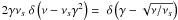
Assuming that the Compton peak is mainly a result of SSC radiation one finds for the ratio
of the luminosities of the peaks (Schlickeiser et al. 2010, hereafter referred to as SBM)
 (1)Since
SSC cooling relies on the synchrotron photons of the same electrons, the electron density
n(γ) is the same in both cases. Similarly, the Doppler
boosting factors are also identical (Dermer & Schlickeiser 2002), which means that the ratio of the luminosities directly reflects
the ratio of the cooling factors
(1)Since
SSC cooling relies on the synchrotron photons of the same electrons, the electron density
n(γ) is the same in both cases. Similarly, the Doppler
boosting factors are also identical (Dermer & Schlickeiser 2002), which means that the ratio of the luminosities directly reflects
the ratio of the cooling factors  (with
i ∈ { SSC,SYN } ). Hence, a dominance of the Compton
peak over the synchrotron peak implies that the electrons mainly cool by inverse Compton
collisions with their self-made photons. In this case, the linear synchrotron cooling has to
be replaced by another cooling process dealing with SSC radiation, which has been considered
by RS.
(with
i ∈ { SSC,SYN } ). Hence, a dominance of the Compton
peak over the synchrotron peak implies that the electrons mainly cool by inverse Compton
collisions with their self-made photons. In this case, the linear synchrotron cooling has to
be replaced by another cooling process dealing with SSC radiation, which has been considered
by RS.
It is important to notice that the nonlinear SSC cooling only operates in the Thomson regime and does not deal with higher order SSC collisions, which are possible. Taking higher oder interactions and/or the Klein-Nishina (KN) regime into account, would lead to a much more complicated approach. If KN effects are important in the beginning, our approach would be at least a good approximation for later times, since the electrons cool significantly over time and will sooner or later reach the Thomson scattering regime. However, blazar spectral energy distributions (SEDs) normally do not show a third broad component, which would be an indicator of higher order scattering or scattering in the KN domain. This is a hint for the validity of the approach. We notice that this restriction to the Thomson regime requires according to RS that the maximum Lorentz factor is not larger than γmax ≈ 1.94 × 10⁴b − 1/3 (b is the normalized magnetic field strength in units of Gauss).
1.1. The model
RS applied the nonlinear SSC model to the simple but illustrative case of mono-energetic
electrons that are instantaneously injected into the jet. It is the purpose of this work
to apply this new model to a slightly more realistic scenario. We assume a spherical,
uniform, nonthermal source with an instantaneous injection of power-law distributed
electrons of the form  . This
describes a single flare event, in which one population of electrons is injected into the
jet and causes a sudden outburst of radiation.
. This
describes a single flare event, in which one population of electrons is injected into the
jet and causes a sudden outburst of radiation.
Such homogeneous one-zone models have been applied with remarkable success to relativistic outflows of TeV blazars or even afterglows of gamma-ray bursts. However, these kind of models lack some details, which could be important. The source need not necessarily be spherical. The electrons could be accelerated at a shock front, which would yield a shell-like form of the source. Also diffusion processes of the ultra-relativistic electrons could allow them to escape the jet, and, thus, being lost to the cooling and radiation processes. Similarly, we neglect the conical structure of the jet, which could result in non-radiating adiabatic energy losses.
In order to avoid effects of time retardation (Eichmann et al. 2010) the evolution of the source is supposed to be on a time-scale that is shorter than the light-crossing time.
Lastly, we treat only the optically thin case here.
1.2. The outline of the paper
We will begin with the calculation of the electron number densities in the linear and nonlinear case in Sect. 2. We will also discuss the temporal evolution of the respective electron densities and will outline their behavior by evaluating the upper and lower cut-offs of the spectra. We will show that any non-linear cooling will ultimately become linear after some time, which requires a treatment with both cooling scenarios in one equation. This has been carried out for mono-energetic electrons by SBM, and we will extend their research here, as well, in Sect. 3.
Sections 4–6 are devoted to the calculation of the total linear and nonlinear synchrotron fluence and the fluence of the combined cooling scenario, respectively. We will discuss our results in Sect. 7.
2. Linear and non-linear electron number densities
In this section we calculate the distribution function of the cooled electrons for linear synchrotron and nonlinear SSC cooling, respectively, and discuss their temporal evolution.
The electron number density n(γ,t) is governed by the
competition between time-varying energy losses and the injection of relativistic electrons
into the jet. This competition is described by the partial differential equation (Kardashev
1962) ![Mathematical equation: \begin{eqnarray} \label{eldispde}\frac{\pd{n(\gamma,t)}}{\pd{t}}-\frac{\pd}{\pd{\gamma}}\left[ |\dot{\gamma}|n(\gamma,t) \right] = Q(\gamma,t). \end{eqnarray}](/articles/aa/full_html/2010/16/aa15284-10/aa15284-10-eq20.png) (2)Q(γ,t)
is the injection rate and we assume an instantaneous injection of power-law distributed
electrons in the form
(2)Q(γ,t)
is the injection rate and we assume an instantaneous injection of power-law distributed
electrons in the form  (3)where
s is the spectral index, γ1 and
γ2 are the lower and upper cut-offs of the electron spectrum,
respectively, H[x] denotes Heaviside’s step function, and
(3)where
s is the spectral index, γ1 and
γ2 are the lower and upper cut-offs of the electron spectrum,
respectively, H[x] denotes Heaviside’s step function, and
 is Dirac’s
δ-distribution.
is Dirac’s
δ-distribution.
2.1. Linear cooling
The linear cooling is described by the linear energy loss term  (4)where
UB = B2/8π
is the magnetic energy density of a magnetic field
B = b G. Schlickeiser & Lerche (2008) obtained the solution for the linear cooling:
(4)where
UB = B2/8π
is the magnetic energy density of a magnetic field
B = b G. Schlickeiser & Lerche (2008) obtained the solution for the linear cooling:
 (5)The
temporal evolution (with
y = A0t, and
A0 defined in the next subsection) of this solution is shown
in Figs. 1–3 for
three different cases of s.
(5)The
temporal evolution (with
y = A0t, and
A0 defined in the next subsection) of this solution is shown
in Figs. 1–3 for
three different cases of s.
 |
Fig. 1 Linear electron distribution for s = 1.5 at four different times y for the initial values: γ1 = 101, and γ2 = 104. |
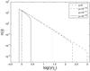 |
Fig. 2 Linear electron distribution for s = 2.5 at four different times y for the initial values: γ1 = 101, and γ2 = 104. |
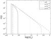 |
Fig. 3 Linear electron distribution for s = 3.5 at four different times y for the initial values: γ1 = 101, and γ2 = 104. |
2.2. Nonlinear cooling
According to RS the nonlinear SSC cooling rate is defined by  (6)with
the constant
(6)with
the constant  . Here σT
is the Thomson cross-section of electron scattering, R is the radius of
the spherical source,
. Here σT
is the Thomson cross-section of electron scattering, R is the radius of
the spherical source,  eV-1 s-1,
Ek = 1.16 × 10⁻⁸b eV,
c1 ≈ 0.684, and
mc2 is the rest-mass energy of an electron.
eV-1 s-1,
Ek = 1.16 × 10⁻⁸b eV,
c1 ≈ 0.684, and
mc2 is the rest-mass energy of an electron.
The integral over the electron number density n(γ,t) basically introduces a time dependence of the cooling rate. This is reasonable, since cooler electrons have less energy they can transfer to the photons, which implies that the electrons do not cool effectively any more.
The solution to the differential Eq. (2)
is derived in Appendix A, and becomes 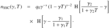 (7)The
implicit time variable T is defined by the nonlinear differential
equation
(7)The
implicit time variable T is defined by the nonlinear differential
equation 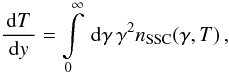 (8)where
y = A0t. As we will see
later the derivative of T with respect to y is as
important as the complete time variable T itself in order to calculate
the synchrotron spectra (cf. Sect. 5). The
calculation of the former is presented in Appendix B, and becomes for s > 3
(8)where
y = A0t. As we will see
later the derivative of T with respect to y is as
important as the complete time variable T itself in order to calculate
the synchrotron spectra (cf. Sect. 5). The
calculation of the former is presented in Appendix B, and becomes for s > 3 ![Mathematical equation: \begin{eqnarray} \label{impltimesol1} U(x) = \left\{ \begin{array}{ll} U_0 \left[ 1-g_2^{3-s} \right], \quad 0\leq x\leq g_2^{-1} \\ U_0 \left[ 1-\frac{2x^{s-3}}{s-1}-\frac{s-3}{s-1}\frac{g_2^{1-s}}{x^2} \right], \quad g_2^{-1}\leq x \leq 1 \\ U_0 \frac{s-3}{(s-1)x^2}\left[ 1-g_2^{1-s} \right],\quad x\geq 1, \end{array} \right. \end{eqnarray}](/articles/aa/full_html/2010/16/aa15284-10/aa15284-10-eq56.png) (9)and
for 1 < s < 3
(9)and
for 1 < s < 3
![Mathematical equation: \begin{eqnarray} \label{impltimesol2} U(x) = \left\{ \begin{array}{ll} U_1 \left[ g_2^{3-s}-1 \right], \quad 0\leq x\leq g_2^{-1} \\ U_1 \left[ \frac{2x^{s-3}}{s-1}-1-\frac{s-3}{s-1}\frac{g_2^{1-s}}{x^2} \right], \quad g_2^{-1}\leq x\leq 1 \\ U_1 \frac{3-s}{(s-1)x^2}\left[ 1-g_2^{1-s} \right], \quad x\geq 1, \end{array} \right. \end{eqnarray}](/articles/aa/full_html/2010/16/aa15284-10/aa15284-10-eq58.png) (10)with
the new time variable
x = γ1T, the ratio between
the initial cut-offs
g2 = γ2/γ1,
and the constants
(10)with
the new time variable
x = γ1T, the ratio between
the initial cut-offs
g2 = γ2/γ1,
and the constants  , and
, and

2.2.1. Temporal evolution of the nonlinear electron number density
If one is interested in the actual temporal evolution of the electron distribution, one
has to perform the integration of U(x) with respect to
the time-variable, yielding for s > 3
![Mathematical equation: \begin{eqnarray} \label{timevabsol1} x(y) = \left\{ \begin{array}{ll} \gamma_1 U_0 \left[ 1-g_2^{3-s} \right] y, \quad 0\leq y\leq y_1\\ \gamma_1 U_0 \left[ y-c_2 \right], \quad y_1 \leq y \leq y_2\\ \left[ 3\gamma_1 U_0 \frac{s-3}{s-1} (1-g_2^{1-s})(y-c_3) \right]^{1/3}, \quad y \geq y_2, \end{array} \right. \end{eqnarray}](/articles/aa/full_html/2010/16/aa15284-10/aa15284-10-eq64.png) (11)and
for 1 < s < 3
(11)and
for 1 < s < 3
![Mathematical equation: \begin{eqnarray} \label{timevabsol2} x(y) = \left\{ \begin{array}{ll} \gamma_1 U_1 \left[ g_2^{3-s}-1 \right]y, \quad 0\leq y\leq y_3 \\ \left[ 2\gamma_1 U_1 \frac{4-s}{s-1}(y-c_5) \right]^{\frac{1}{4-s}},\quad y_3\leq y\leq y_4 \\ \left[ 3\gamma_1 U_1 \frac{3-s}{s-1}(1-g_2^{1-s})(y-c_6) \right]^{1/3} , \quad x\geq y_4, \end{array} \right. \end{eqnarray}](/articles/aa/full_html/2010/16/aa15284-10/aa15284-10-eq65.png) (12)The
integration and the approximations used for it can be found in Appendix C. The time limits
yi and the constants
ci are chosen in such a way that the
solution x(y) is continuous for all
y. The values are also listed in Appendix C.
(12)The
integration and the approximations used for it can be found in Appendix C. The time limits
yi and the constants
ci are chosen in such a way that the
solution x(y) is continuous for all
y. The values are also listed in Appendix C.
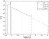 |
Fig. 4 Nonlinear electron distribution for s = 1.5 at four different times y for the initial values: γ1 = 101, and γ2 = 104. |
 |
Fig. 5 Nonlinear electron distribution for s = 2.5 at four different times y for the initial values: γ1 = 101, and γ2 = 104. |
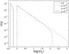 |
Fig. 6 Nonlinear electron distribution for s = 3.5 at four different times y for the initial values: γ1 = 101, and γ2 = 104. |
In Figs. 4–6 we plotted the time evolution of the nonlinear electron spectrum for s = 1.5, s = 2.5, and s = 3.5, respectively.
As one can see, the spectrum cools significantly faster for harder spectra (smaller spectral index). It is also quite obvious that the spectrum contracts relatively rapidly, which means that for late times the spectrum is identical to a δ-function (cf. next subsection). One should also notice the increasing pile-up for s < 2 at the upper limit for later times, which becomes a drop for larger s, similarly to the linear case.
2.3. Temporal evolution of the cut-offs
The qualitative behavior outlined in the last subsections of the electron densities is confirmed by Fig. 7 showing the time dependence of the upper and lower cut-offs defined by the Heaviside functions of the respective electron densities.
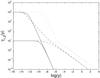 |
Fig. 7 Time dependence of the upper (γ2, upper curves) and lower (γ1, lower curves) cut-offs of the electron spectra, respectively, for the standard values γ1 = 101, γ2 = 104, R15 = 1, and q5 = 1. Full curve: linear electron cooling for s = 2. Dashed curve: nonlinear electron cooling for s = 2. Dotted curve: nonlinear electron cooling for s = 3.5. |
Concerning the linear cooling case, we find that once the cooling has begun to be
important, the electrons cool with a y-1-dependence as
expected. Similarly to the nonlinear case, the cooling of the high-energetic electrons
begins a factor of about  earlier than
for the low-energetic ones, resulting again in a δ-function appearance of
the electron spectrum for later times.
earlier than
for the low-energetic ones, resulting again in a δ-function appearance of
the electron spectrum for later times.
In Fig. 7 the linear cooling operates much faster than the nonlinear cooling. This depends critically on the parameters we have chosen for the plot: R = 1015R15 cm, and q0 = 105q5 cm-3. Especially for higher values of these parameters (cf. Fig. 8) the linear cooling begins at much later times for larger R, or the nonlinear cooling begins much earlier for larger q0 (the magnetic field strength does not change the overall result, since both cooling scenarios depend on B2; cf. the definitions of D0 and A0). We note, however, that at one point in time the linear cooling will always dominate over the nonlinear cooling, since it cools faster for later times than the nonlinear case.
This behavior indicates that linear and nonlinear cooling should not be treated separately, as we did in this section. This fact has been treated by SBM for the illustrative case of mono-energetic electrons (at all times). We will calculate the number density of the combined linear and non-linear cooled (hereafter referred to as “combined” cooled) electrons in the next section.
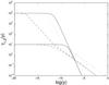 |
Fig. 8 The same as in Fig. 7, but with R15 = 10, and q5 = 104. Note the different values on the horizontal axis. |
3. Combined cooled electron number density
The combined cooling is described by the energy loss term  (13)with
K0 = D0/A0.
(13)with
K0 = D0/A0.
Inserting this into Eq. (2) yields the
solution 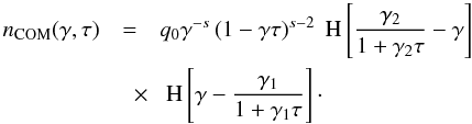 (14)The
similarity of Eq. (14) with (7) is not surprising, since the way to derive the
solution is the same in both ways. The important difference is that the implicit time
variable T has changed to the new definition τ:
(14)The
similarity of Eq. (14) with (7) is not surprising, since the way to derive the
solution is the same in both ways. The important difference is that the implicit time
variable T has changed to the new definition τ:
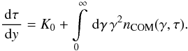 (15)In
Appendix D we derive the complete solution of the
implicit time variable
(15)In
Appendix D we derive the complete solution of the
implicit time variable  , which becomes for
s > 3
, which becomes for
s > 3 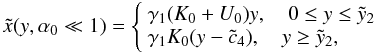 (16)
(16)![Mathematical equation: \begin{eqnarray} \label{comtimevabsol2} \xc(y,\alpha_0\gg 1)= \left\{ \begin{array}{ll} \gamma_1 (K_0+U_0) y, \quad 0\leq y\leq \yc_2 \\ \left[ 3 \alpha_0^2 \gamma_1 K_0 (y-\cc_5) \right]^{1/3}, \quad \yc_2 \leq y\leq \yc_3 \\ \gamma_1 K_0 (y-\cc_6),\quad y\geq\yc_3, \end{array} \right. \end{eqnarray}](/articles/aa/full_html/2010/16/aa15284-10/aa15284-10-eq91.png) (17)and
for 1 < s < 3
(17)and
for 1 < s < 3 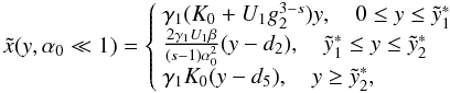 (18)
(18)![Mathematical equation: \begin{eqnarray} \label{comtimevabsol4} \xc(y,\alpha_0\gg 1)= \left\{ \begin{array}{ll} \gamma_1 (K_0+U_1 g_2^{3-s}) y , \quad 0\leq y\leq \ys_1 \\ \left[ \frac{2\gamma_1 U_1 (4-s)}{(s-1)}(y-d_3) \right]^{\frac{1}{4-s}}, \quad \ys_1\leq y\leq \ys_3 \\ \left[ 3\alpha_0^2\gamma_1 K_0 (y-d_6) \right]^{1/3}, \quad \ys_3 \leq y\leq \ys_4 \\ \gamma_1 K_0 (y-d_7), \quad y\geq\ys_4, \end{array} \right. \end{eqnarray}](/articles/aa/full_html/2010/16/aa15284-10/aa15284-10-eq93.png) (19)The
approximations and the values of the constants
(19)The
approximations and the values of the constants  ,
,
 ,
,
 , and
di can be found in Appendix D, as well. They are chosen in such a way that
, and
di can be found in Appendix D, as well. They are chosen in such a way that
 is continuous for all
times. There we also introduce
is continuous for all
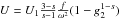
times. There we also introduce 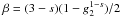 and the important injection parameter
 (20)for
extended power law injection spectra. The power law injection parameter
α0 depends on the particle number density
q0, the initial lower cut-off γ1,
the electron spectral index s, the constant K0,
and only weakly on the upper cut-off, since
(20)for
extended power law injection spectra. The power law injection parameter
α0 depends on the particle number density
q0, the initial lower cut-off γ1,
the electron spectral index s, the constant K0,
and only weakly on the upper cut-off, since  .
.
3.1. Power law injection parameter
For standard blazar parameters
q0 = 105q5 cm-3
and R = 1015R15 cm we use from SBM
(K0/q0)1/2 = 106(R15q5) − 1/2
and introduce the total number of instantaneously injected electrons 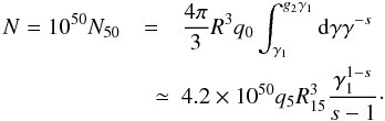 (21)yielding
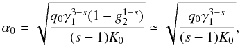
 , so that the power law injection parameter
becomes
, so that the power law injection parameter
becomes  (22)in
terms of the characteristic Lorentz factor introduced by SBM
(22)in
terms of the characteristic Lorentz factor introduced by SBM  (23)The
injection parameter is determined by the total number of injected electrons and the size
of the source as indicated, but independent of the magnetic field strength. If the lower
cutoff of the injected power law γ1 is higher (smaller) than
γB, the injection parameter
α0 will be larger (smaller) than unity. For a compact source
with a large number of injected electrons, the injection parameter is much larger than
unity.
(23)The
injection parameter is determined by the total number of injected electrons and the size
of the source as indicated, but independent of the magnetic field strength. If the lower
cutoff of the injected power law γ1 is higher (smaller) than
γB, the injection parameter
α0 will be larger (smaller) than unity. For a compact source
with a large number of injected electrons, the injection parameter is much larger than
unity.
Basically the injection parameter is the fundamental ordering parameter that defines the ratio between the magnitudes of the synchrotron and the Compton peak. An injection parameter smaller than unity corresponds to a higher synchrotron flux compared to the Compton flux leading to the linear synchrotron cooling of the electrons, as one can see in Eqs. (16) and (18). Similarly, an injection parameter being larger than unity leads to the non-linear SSC cooling shown in Eqs. (17) and (19), since the flux of the Compton peak is higher than of the synchrotron peak, which was the condition for the non-linear cooling. One should note, however, that our remarks from the previous section hold: Any non-linear cooling will sooner or later turn into linear cooling.
It is also noteworthy that α0 is independent of the magnetic field strength. This results from the same dependence of both, A0 and D0, on b2.
3.2. Temporal evolution of the combined electron number density
As we did in the separated cases we also present here the temporal evolution of nCOM. We will begin with the case α0 ≪ 1 and then proceed with the opposite case.
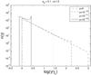 |
Fig. 9 Temporal evolution of the combined electron number density for s = 1.5 and α0 = 0.1 at four different times y with the initial values γ1 = 10 and γ2 = 104. |
 |
Fig. 10 Temporal evolution of the combined electron number density for s = 2.5 and α0 = 0.1 at four different times y with the initial values γ1 = 10 and γ2 = 104. |
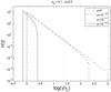 |
Fig. 11 Temporal evolution of the combined electron number density for s = 3.5 and α0 = 0.1 at four different times y with the initial values γ1 = 10 and γ2 = 104. |
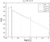 |
Fig. 12 Temporal evolution of the combined electron number density for s = 1.5 and α0 = 100 at four different times y with the initial values γ1 = 10 and γ2 = 104. |
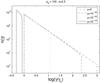 |
Fig. 13 Temporal evolution of the combined electron number density for s = 2.5 and α0 = 100 at four different times y with the initial values γ1 = 10 and γ2 = 104. |
 |
Fig. 14 Temporal evolution of the combined electron number density for s = 3.5 and α0 = 100 at four different times y with the initial values γ1 = 10 and γ2 = 104. |
3.3. Temporal evolution of the cut-offs
In this section we want to verify the results of the last section, especially of the temporal behavior of the electron distribution. Therefore, we discuss the evolution of the cut-offs for three different cases of s shown in Figs. 15 and 16.
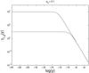 |
Fig. 15 Temporal evolution of the cut-offs of the combined electron number density for s = 2.0 and α0 = 0.1 for the initial values γ1 = 10 and γ2 = 104. |
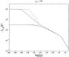 |
Fig. 16 Temporal evolution of the cut-offs of the combined electron number density for s = 2.0 (full curve), s = 3.5 (dashed curve) and α0 = 100 for the initial values γ1 = 10 and γ2 = 104. |
Since for α0 ≪ 1 the behavior of the cut-offs is independent of s, we only plotted one case in Fig. 15. It is obvious that this is indeed very similar to the linear solution of Sect. 2.1 (with the plot of the cut-offs in Sect. 2.3).
For α0 ≫ 1 we notice that the cooling begins much earlier than in the other case, with the hard case beginning even two orders of magnitude earlier in the example shown here than the soft case. We also notice that the soft case cools linearly in the beginning until it merges again with the already non-linearly cooled hard case (here, at roughly y ≈ 10-14). Interestingly, from that moment on both cases cool the same. When both begin to cool linearly again at late times (at about y > 10-8) they match the cooling of the case with α0 ≪ 1.
Obviously, the electron distributions of all cases undergo severe quenching resulting in the appearance of a δ-function for later times.
Overall we can say that the behavior of the combined cooling is similar to the respective cases of the separated cooling scenarios. In order to stress the most important point once more, the non-linear case turns linear at late times as we expected (cf. Sect. 2.3).
4. Linear synchrotron fluence
In the next three sections we will derive the synchrotron fluence spectra, for which we need at first the respective intensity spectra. We use the monochromatic approximation of the synchrotron power introduced by Felten & Morrison (1966). This form is mathematically convenient, but will lead to more distinctive spectral breaks in the resulting spectrum as if one would use the general form of the synchrotron power of Crusius & Schlickeiser (1988). One should note, however, that the derived power-laws in the resulting spectrum using the monochromatic approximation should also be visible in a spectrum obtained with the general form. Similarly, since due to the cooling the electron distribution becomes like a δ-function (cf. Sects. 2 and 3) for later times, the result in this regime should not differ significantly between the respective forms. As we will see later, for late times, i.e. low frequencies, the results of this work match those of RS and SBM, which used the general form of the synchrotron power.
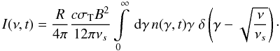
Thus, the synchrotron intensity spectrum of a homogeneous, spherical, optically thin source
is in the monochromatic approximation given by  (24)where
ν is the frequency of the emitted photon. The characteristic frequency is
defined by
(24)where
ν is the frequency of the emitted photon. The characteristic frequency is
defined by  Hz.
Hz.
We can use the substitution rule for δ-functions, providing
 .
Inserting this into Eq. (24) results in:
.
Inserting this into Eq. (24) results in:
 (25)If
we now apply this to the linear electron distribution Eq. (5), define the normalized frequency
(25)If
we now apply this to the linear electron distribution Eq. (5), define the normalized frequency  ,
and a new time variable
,
and a new time variable  , we obtain
 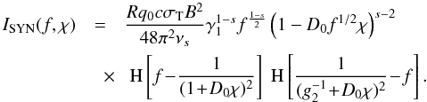 (26)The
fluence is the time-integrated intensity spectrum. Setting an arbitrary upper limit would
result in the fractional fluence, which shows the fluence after some time. Here we treat,
however, only the total fluence with an upper limit that is infinite. Thus,
(26)The
fluence is the time-integrated intensity spectrum. Setting an arbitrary upper limit would
result in the fractional fluence, which shows the fluence after some time. Here we treat,
however, only the total fluence with an upper limit that is infinite. Thus,  (27)Introducing
the variable
Ω = D0f1/2χ
we yield
(27)Introducing
the variable
Ω = D0f1/2χ
we yield  (28)The
result of this integral gives two different frequency regimes, and can be written as
(28)The
result of this integral gives two different frequency regimes, and can be written as
 (29)with

This is the well known result that has been obtained by Schlickeiser & Lerche
(2008), too. The important points of this result
are that the fluence is independent of the spectral index s of the electron
injection rate for frequencies smaller than unity following a power-law with a spectral
index ϑSYN = 1/2. At f = 1
the spectrum exhibits a break to a steeper spectrum with  depending on
s. The spectrum is cut off at
depending on
s. The spectrum is cut off at  .
.
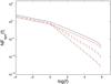 |
Fig. 17 NFSYN as a function of f for three cases of s (full: s = 2, dashed: s = 3, dot-dashed: s = 4) and for g2 = 103. The red lines indicate the analytical solution Eq. (29) with an offset of 10-0.7. |
In Fig. 17 we show the numerical solution of the fluence spectrum for which we normalized the fluence by NFSYN = FSYN/Nl. We plotted the result for g2 = 103 and three values of s. We also plotted the analytical results, but with a small offset in order to highlight them.
As one can see, the numerical and the analytical result match each other rather well, which is not so surprising, since we introduced no strong approximations during the analytical work.
5. Nonlinear synchrotron fluence
In order to obtain the intensity spectrum and the fluence of the nonlinear case we have to
insert the nonlinear electron distribution Eq. (7) into (25), yielding
 (30)Integrating
this with respect to time yields the total fluence:
(30)Integrating
this with respect to time yields the total fluence: 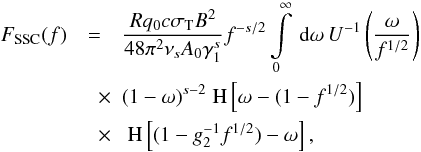 (31)for
which we used the substitution
ω = f1/2x.
(31)for
which we used the substitution
ω = f1/2x.
Since we must take care of the spectral index s, we split the ongoing discussion into two parts for each case of the spectral index.
5.1. Large spectral index
We begin with the spectral index being larger than 3. Then, the first integral we have to
calculate is for the case  , where
 , yielding
 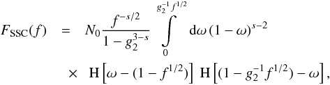 (32)where
we set
(32)where
we set 
The integration can be easily performed giving, according to the Heaviside functions,
solutions for two regimes of the normalized frequency: 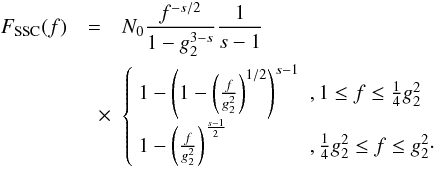 (33)The
intermediate ω-range (
(33)The
intermediate ω-range ( ) is the next case we have
to consider. Here
) is the next case we have
to consider. Here ![Mathematical equation: \begin{eqnarray} U(\omega)=U_0\left[ 1-\frac{2(\omega/f^{1/2})^{s-3}}{s-1}-\frac{s-3}{s-1}\frac{g_2^{1-s}}{(\omega/f^{1/2})^2} \right] \cdot \end{eqnarray}](/articles/aa/full_html/2010/16/aa15284-10/aa15284-10-eq154.png) (34)Approximating
this with the leading term, which is valid for most parts of the time period and for
spectral indices not too close to 3 (cf. Fig. C.1 in
Appendix C), the integral becomes
(34)Approximating
this with the leading term, which is valid for most parts of the time period and for
spectral indices not too close to 3 (cf. Fig. C.1 in
Appendix C), the integral becomes 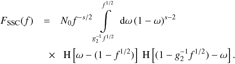 (35)This
is again easily solved for two regimes of f obtained from the Heaviside
functions and indicated below. We find
(35)This
is again easily solved for two regimes of f obtained from the Heaviside
functions and indicated below. We find 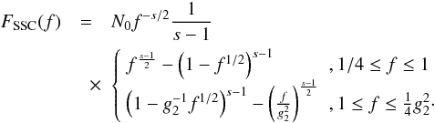 (36)The
third time regime ω ≥ f1/2
requires
(36)The
third time regime ω ≥ f1/2
requires 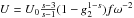 , for which the
fluence becomes
, for which the
fluence becomes  (37)The
primitive of the integral can be obtained by two integration by parts, yielding for
arbitrary limits a and b, which need to be specified by
the Heaviside functions later,
(37)The
primitive of the integral can be obtained by two integration by parts, yielding for
arbitrary limits a and b, which need to be specified by
the Heaviside functions later, ![Mathematical equation: \begin{eqnarray} \label{int3prim} \mathrm{INT} &=& \intl_{a}^{b}\td{\omega}\omega^2(1-\omega)^{s-2} \nonumber \\ &=&\left[ -\frac{\omega^2}{s-1}(1-\omega)^{s-1} \right]_a^b + \left[ -\frac{2\omega}{s^2-s}(1-\omega)^s \right]_a^b \nonumber \\ &\quad +& \left[ -\frac{2}{s^3-s}(1-\omega)^{s+1} \right]_a^b. \end{eqnarray}](/articles/aa/full_html/2010/16/aa15284-10/aa15284-10-eq161.png) (38)For
f ≤ 1/4 the limits become
a = 1 − f1/2 and
(38)For
f ≤ 1/4 the limits become
a = 1 − f1/2 and
 . Assuming g2 ≫ 1
we can neglect the negative terms, which are the terms where we inserted the upper limit.
Since f ≤ 1/4 we see that the second and third of the
remaining terms are also much reduced compared to the first one. Thus, we approximate the
integral with
. Assuming g2 ≫ 1
we can neglect the negative terms, which are the terms where we inserted the upper limit.
Since f ≤ 1/4 we see that the second and third of the
remaining terms are also much reduced compared to the first one. Thus, we approximate the
integral with  (39)From
the Heaviside functions of Eq. (37) we
obtain another frequency regime located between
1/4 ≤ f ≤ 1. The limits in this case become
a = f1/2 and
(39)From
the Heaviside functions of Eq. (37) we
obtain another frequency regime located between
1/4 ≤ f ≤ 1. The limits in this case become
a = f1/2 and
 . Using the same
approximation as above, for which we note however that these approximations are not as
well fitting as in the previous case, we find
. Using the same
approximation as above, for which we note however that these approximations are not as
well fitting as in the previous case, we find  (40)Thus,
we yield in the late time case for the fluence
(40)Thus,
we yield in the late time case for the fluence  (41)Collecting
terms we find for the total fluence with a large spectral index
s > 3
(41)Collecting
terms we find for the total fluence with a large spectral index
s > 3
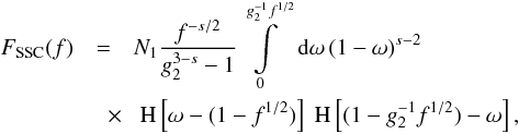
![Mathematical equation: \begin{eqnarray} F_{\rm SSC}(f)&=&N_0\left[ F_1(f< 1/4)+F_2(1/4\leq f< 1) \right. \nonumber \\ &\quad + & \left. F_3(1\leq f<\frac{1}{4}g_2^2)+F_4(\frac{1}{4}g_2^2\leq f\leq g_2^2) \right], \end{eqnarray}](/articles/aa/full_html/2010/16/aa15284-10/aa15284-10-eq172.png) (42)with
the terms
(42)with
the terms ![Mathematical equation: \begin{eqnarray} \label{fsynsscs3p1} F_1 &=& \frac{(1-f^{1/2})^2}{(s-3)(1-g_2^{1-s})}f^{-3/2} \\ F_2 &=& \frac{f^{-s/2}}{s-1}\left[ f^{\frac{s-1}{2}}-(1-f^{1/2})^{s-1} \right] \nonumber \\ \label{fsynsscs3p2} & \quad +& \frac{f^{-s/2}}{(s-3)(1-g_2^{1-s})}(1-f^{1/2})^{s-1} \\ F_3 &=& \frac{f^{-s/2}}{(s-1)(1-g_2^{3-s})} \left[ 1-\left( 1-\left( \frac{f}{g_2^2} \right)^{1/2} \right)^{s-1} \right] \nonumber \\ & \quad +& \frac{f^{-s/2}}{s-1} \left[ \left( 1-\left( \frac{f}{g_2^2} \right)^{1/2} \right)^{s-1} - \left( \frac{f}{g_2^2} \right)^{\frac{s-1}{2}} \right] \nonumber \\ \label{fsynsscs3p3} &\quad \approx & \frac{f^{-s/2}}{s-1} \left[ 1-\left( \frac{f}{g_2^2} \right)^{\frac{s-1}{2}} \right] \\ \label{fsynsscs3p4} F_4 &=& \frac{f^{-s/2}}{(s-1)(1-g_2^{3-s})} \left[ 1-\left( \frac{f}{g_2^2} \right)^{\frac{s-1}{2}} \right]\cdot \end{eqnarray}](/articles/aa/full_html/2010/16/aa15284-10/aa15284-10-eq173.png) In
the third part we approximated again for g2 ≫ 1. If we do
the same in the fourth part, the third and fourth part would be the same and could be
merged. This does not change much to the overall result, which should be discussed
briefly.
In
the third part we approximated again for g2 ≫ 1. If we do
the same in the fourth part, the third and fourth part would be the same and could be
merged. This does not change much to the overall result, which should be discussed
briefly.
The fluence behaves like a power-law with a constant spectral index
ϑSSC = 3/2 for f ≤ 1,
independently of s, which is steeper than in the case of linear cooling.
At f ≈ 1 the spectrum exhibits a spectral break to a steeper power-law
with a change in the spectral index of
ΔϑSSC = (s − 3)/2. At a
frequency the spectrum is cut off at
the high energy end.
 |
Fig. 18 NFSSC as a function of f for three cases of s > 3 full: s = 3.1, dashed: s = 4, dot-dashed: s = 5) and for g2 = 103. The red lines indicate the analytical solution Eqs. (43)–(46) with an offset of 10-0.9. |
Obviously for most parts of f the analytical result and the numerical result match each other. However, for 1/4 ≤ f < 1 there is a discrepancy between the results, which is also quite obvious, since the analytical result is not continuous at f = 1/4. We already indicated during the analytical calculations that the approximation for the second part (Eq. (44)) could be invalid. One can also see that the approximation in the third part (Eq. (45)) becomes less valid for s → 3. Thus, the numerical result confirms the expectations we mentioned during the derivation of the analytical result.
5.2. Small spectral index
Now, we want to deal with the fluence for electron spectral indices 1 < s < 3. As a matter of fact, the steps are quite similar to the case before, but nonetheless we will repeat them here.
We begin again with the case , where
 :
:  (47)with
the definition
(47)with
the definition  .
Since the integral is easily obtained once more, for small ω the fluence
becomes
.
Since the integral is easily obtained once more, for small ω the fluence
becomes 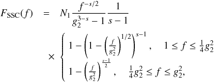 (48)where
the Heaviside functions of Eq. (47)
defined the frequency regimes.
(48)where
the Heaviside functions of Eq. (47)
defined the frequency regimes.
The intermediate ω-range ( ) is the next case we turn
our attention to. Here
) is the next case we turn
our attention to. Here ![Mathematical equation: \begin{eqnarray} U(\omega)=U_1\left[ \frac{2(\omega/f^{1/2})^{s-3}}{s-1}-1+\frac{3-s}{s-1}\frac{g_2^{1-s}}{(\omega/f^{1/2})^2} \right] \cdot \end{eqnarray}](/articles/aa/full_html/2010/16/aa15284-10/aa15284-10-eq191.png) (49)Taking
into account only the leading term of U(ω) (the validity
of this approximation is shown in Fig. C.2 in
Appendix C), as we did in the same case for the
steep electron spectrum, we obtain
(49)Taking
into account only the leading term of U(ω) (the validity
of this approximation is shown in Fig. C.2 in
Appendix C), as we did in the same case for the
steep electron spectrum, we obtain 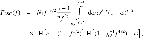 (50)this
integral can be expressed in terms of the hypergeometric function, yielding no simple
solution. Thus, for intermediate frequencies we cannot present an analytical solution.
(50)this
integral can be expressed in terms of the hypergeometric function, yielding no simple
solution. Thus, for intermediate frequencies we cannot present an analytical solution.
Finally, we have to turn our attention to the late time regime, which means
ω ≥ f1/2. Here
 , for which the fluence becomes
 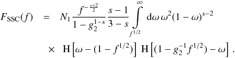 (51)This
is almost the same integral that we solved in the case of
s > 3, thus we can use the same primitive
(Eq. (38)). In fact, the limits and the
frequency regimes are the same as in the case of steeply injected electrons. Therefore,
using the same approximations as we did in that case, we obtain the solution for
f ≤ 1/4
(51)This
is almost the same integral that we solved in the case of
s > 3, thus we can use the same primitive
(Eq. (38)). In fact, the limits and the
frequency regimes are the same as in the case of steeply injected electrons. Therefore,
using the same approximations as we did in that case, we obtain the solution for
f ≤ 1/4 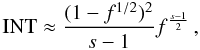 (52)and
for 1/4 ≤ f ≤ 1
(52)and
for 1/4 ≤ f ≤ 1 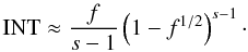 (53)Collecting
terms, we find the fluence for large ω:
(53)Collecting
terms, we find the fluence for large ω: 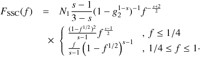 (54)Now,
we have performed all necessary steps to calculate the synchrotron fluence of SSC cooled
electrons that are injected into the jet with a spectral index
1 < s < 3. Therefore,
(54)Now,
we have performed all necessary steps to calculate the synchrotron fluence of SSC cooled
electrons that are injected into the jet with a spectral index
1 < s < 3. Therefore,
![Mathematical equation: \begin{eqnarray} F_{\rm SSC}(f) = N_1 \left[ F_5(f< 1/4)+F_6 \left(\frac{1}{4}g_2^2\leq f\leq g_2^2\right) \right], \end{eqnarray}](/articles/aa/full_html/2010/16/aa15284-10/aa15284-10-eq199.png) (55)with
(55)with
![Mathematical equation: \begin{eqnarray} \label{fsynssc1s3p1} F_5 &=& \frac{(1-f^{1/2})^2}{(3-s)(1-g_2^{1-s})}f^{-3/2} \\ \label{fsynssc1s3p4} F_6 &=& \frac{f^{-s/2}}{(s-1)(g_2^{3-s}-1)} \left[ 1-\left( \frac{f}{g_2^2} \right)^{\frac{s-1}{2}} \right]\cdot \end{eqnarray}](/articles/aa/full_html/2010/16/aa15284-10/aa15284-10-eq200.png) We
do not present the results for the intermediate frequency regime
We
do not present the results for the intermediate frequency regime  , because this is the part
where the intermediate ω-regime is also important, if not more important
than the contributions of the early and late ω-regimes. And for that part
we did not obtain an analytical solution.
, because this is the part
where the intermediate ω-regime is also important, if not more important
than the contributions of the early and late ω-regimes. And for that part
we did not obtain an analytical solution.
However, the results in the other frequency parts are noteworthy. The fluence for flat
injected electron spectra shows similar characteristics as the fluence for steep injected
electrons. We find, again, that the spectral index does not depend on s
for frequencies f < 1/4 and
has the same value ϑSSC = 3/2. There is
also a cut-off for high frequencies at .
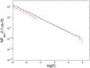 |
Fig. 19 NFSSC as a function of f for three cases of s > 3 (full: s = 3.1, dashed: s = 4, dot-dashed: s = 5) and for g2 = 103. The red lines indicate the analytical solution Eqs. (56) and (57) with an offset of 10-0.9. |
As one can see, the numerical and the analytical solutions agree very well for the
presented frequency intervals. Interestingly, there is no spectral break in the numerical
result at around f = 1, different from the behavior of steeply injected
electrons. The spectrum is cut off at as expected.
It is noteworthy that the spectrum does not exhibit a break at f = 1, implying that the spectrum for f > 1 does not depend strongly on s, either. It is quite obvious that the offset between the numerical and the analytical solution does not change from the low frequency regime to the high frequency regime near the cut-off. The curves of the analytical plot at the cut-off are also equal for all cases, similar to the numerical result. Especially this last point is different from the steep injection case, where the magnitudes of the curves differ significantly from case to case. These are hints for the validity of the numerical solution exhibiting no break, which is an important difference from the steep injection case.
6. Synchrotron fluence of combined cooled electrons
We will, now, calculate the synchrotron fluence spectrum of electrons undergoing the combined cooling.
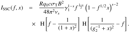
As before, we begin with the intensity by inserting Eq. (14) into (25). With the
same definition for the normalized frequency f we obtain ![Mathematical equation: \begin{eqnarray} \label{intspeccom} I_{\rm COM}(f,\xc)&=&\frac{q_0Rc\sigma_{\rm T} B^2}{48\pi^2\nu_s}\gamma_1^{1-s} f^{\frac{1-s}{2}} \left( 1-f^{1/2}\xc \right)^{s-2} \nonumber \\[-3mm] &\quad \times& \HSF{\frac{1}{(g_2^{-1} +\xc)^2}-f}\HSF{f-\frac{1}{(1+\xc)^2}}\cdot \end{eqnarray}](/articles/aa/full_html/2010/16/aa15284-10/aa15284-10-eq205.png) (58)The
integration with respect to time yields the synchrotron fluence:
(58)The
integration with respect to time yields the synchrotron fluence: 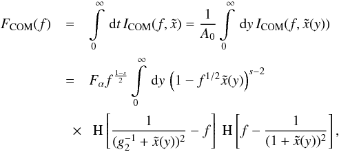 (59)with
the definition
(59)with
the definition  .
.
It is advantageous in this case to use y as the integration variable
instead of , as we did in the
other cases, because we already made a lot of approximations while calculating
 for the discussions in Sect. 3, and it is unnecessary to repeat these steps again.
Using from Eqs. (16)–(19) we will in each
of the following integrations define the new variable  .
.
6.1. Small injection parameter, large spectral index
Here we discuss the case of s > 3 and α0 ≪ 1.
The first regime we have to consider is for 0 ≤ Ψ ≤ Ψ2, with
Ψ2: = Ψ(y2) = f1/2.
With
dΨ = f1/2γ1(K0 + U0)dy
we find ![Mathematical equation: \begin{eqnarray} \label{fs3a01a} \Fc(f)&=&\Fa\frac{f^{-s/2}}{\gamma_1(K_0+U_0)}\intl_0^{\Psi_2}\td{\Psi}(1-\Psi)^{s-2} \nonumber \\ &\quad \times& \HSF{(1-f^{1/2}g_2^{-1})-\Psi}\HSF{\Psi-(1-f^{1/2})} \nonumber \\ &=&\Fa \frac{f^{-s/2}}{\gamma_1(K_0+U_0)(s-1)} \left[ -(1-\Psi)^{s-1} \right]_{a}^{b}, \end{eqnarray}](/articles/aa/full_html/2010/16/aa15284-10/aa15284-10-eq213.png) (60)where
a and b are defined by the limits of the integral and
the Heaviside functions. For f < 1 we find
a = 1 − f1/2 and
b = f1/2, resulting in
(60)where
a and b are defined by the limits of the integral and
the Heaviside functions. For f < 1 we find
a = 1 − f1/2 and
b = f1/2, resulting in
![Mathematical equation: \begin{eqnarray} \label{fs3a01a1} \Fc(f<1)=\Fa \frac{f^{-1/2}}{\gamma_1(K_0+U_0)(s-1)} \nonumber \\ \times \left[ 1-(f^{-1/2}-1)^{s-1} \right] \, , \end{eqnarray}](/articles/aa/full_html/2010/16/aa15284-10/aa15284-10-eq215.png) (61)This
becomes negative for f < 1/4
which is not physically possible, and, therefore, this solution does not contribute for
lower frequencies.
(61)This
becomes negative for f < 1/4
which is not physically possible, and, therefore, this solution does not contribute for
lower frequencies.
For f > 1 we obtain the limits
a = 0 and  ,
resulting in
,
resulting in ![Mathematical equation: \begin{eqnarray} \label{fs3a01a2} \Fc(f>1)=\Fa \frac{f^{-s/2}}{\gamma_1(K_0+U_0)(s-1)} \nonumber \\ \times \left[ 1-\left( \frac{f}{g_2^2} \right)^{\frac{s-1}{2}} \right] \, . \end{eqnarray}](/articles/aa/full_html/2010/16/aa15284-10/aa15284-10-eq218.png) (62)Obviously,
this is cut off at .
(62)Obviously,
this is cut off at .
For Ψ > Ψ2 we find
dΨ = f1/2γ1K0dy,
leading to ![Mathematical equation: \begin{eqnarray} \label{fs3a01b} \Fc(f)&=&\Fa \frac{f^{-s/2}}{\gamma_1K_0}\intl_{\Psi_2}^{\infty}\td{\Psi}(1-\Psi)^{s-2} \nonumber \\ &\quad \times& \HSF{(1-f^{1/2}g_2^{-1})-\Psi}\HSF{\Psi-(1-f^{1/2})} \nonumber \\ &=&\Fa \frac{f^{-s/2}}{\gamma_1K_0(s-1)} \left[ -(1-\Psi)^{s-1} \right]_a^b. \end{eqnarray}](/articles/aa/full_html/2010/16/aa15284-10/aa15284-10-eq221.png) (63)We
find for f < 1/4 that
a = 1 − f1/2 and
, yielding
(63)We
find for f < 1/4 that
a = 1 − f1/2 and
, yielding
![Mathematical equation: \begin{eqnarray} \label{fs3a01b1} \Fc(f<1/4)=\Fa\frac{f^{-1/2}}{\gamma_1K_0(s-1)} \left[ 1-g_2^{1-s} \right] \, . \end{eqnarray}](/articles/aa/full_html/2010/16/aa15284-10/aa15284-10-eq222.png) (64)For
f > 1/4 we obtain for
a = f1/2 and
(64)For
f > 1/4 we obtain for
a = f1/2 and
![Mathematical equation: \begin{eqnarray} \label{fs3a01b2} \Fc(f>1/4)&=&\Fa\frac{f^{-1/2}}{\gamma_1K_0(s-1)} \nonumber \\ &\quad \times& \left[ (f^{-1/2}-1)^{s-1}-g_2^{1-s} \right]\, , \end{eqnarray}](/articles/aa/full_html/2010/16/aa15284-10/aa15284-10-eq224.png) (65)which
becomes negative for f > 1.
(65)which
becomes negative for f > 1.
Collecting terms, we obtain the total fluence ![Mathematical equation: \begin{eqnarray} \label{fs3a01sol} \Fc(s\!>\!3,\alpha_0\ll 1)&=&\Fa \left[ F_{\rm c}^1(f\!<\!1/4)\right. \nonumber \\ &\quad +& \left.F_{\rm c}^2(1/4\!<\!f\!<\!1)\!+\!F_{\rm c}^3(1\!<\!f\!<\!g_2^2) \right]. \end{eqnarray}](/articles/aa/full_html/2010/16/aa15284-10/aa15284-10-eq225.png) (66)with
(66)with
![Mathematical equation: \begin{eqnarray} F_{\rm c}^1 &=& \frac{f^{-1/2}}{\gamma_1K_0(s-1)} \left[ 1-g_2^{1-s} \right] \\ F_{\rm c}^2 &=& \frac{f^{-1/2}}{\gamma_1(s-1)} \left\{ \frac{1}{K_0}\left[ (f^{-1/2}-1)^{s-1}-g_2^{1-s} \right] \right. \nonumber \\ & & \left.+ \frac{1}{K_0+U_0}\left[ 1-(f^{-1/2}-1)^{s-1} \right] \right\} \\ F_{\rm c}^3 &=& \frac{f^{-s/2}}{\gamma_1(K_0+U_0)(s-1)} \left[ 1-\left( \frac{f}{g_2^2} \right)^{\frac{s-1}{2}} \right]\cdot \end{eqnarray}](/articles/aa/full_html/2010/16/aa15284-10/aa15284-10-eq226.png) This
is the expected result. Since the cooling is dominated by the linear part, the solution is
comparable to the linear fluence of Sect. 4
representing a broken power-law with a constant spectral index
(ϑ1 = 1/2) for frequencies below unity,
and a steepening of
Δϑ1 = (s − 1)/2 for
f ≥ 1. The spectrum is cut off at .
This
is the expected result. Since the cooling is dominated by the linear part, the solution is
comparable to the linear fluence of Sect. 4
representing a broken power-law with a constant spectral index
(ϑ1 = 1/2) for frequencies below unity,
and a steepening of
Δϑ1 = (s − 1)/2 for
f ≥ 1. The spectrum is cut off at .
6.2. Small injection parameter, small spectral index
We continue with the case of 1 < s < 3 and α0 ≪ 1.
The first part is  , with
 . In this
case, we find
. In this
case, we find  leading to
 ![Mathematical equation: \begin{eqnarray} \label{f1s3a01a} \Fc(f)&=&\Fa\frac{f^{-s/2}}{\gamma_1(K_0+U_1g_2^{3-s})}\intl_0^{\Psis_1}\td{\Psi}(1-\Psi)^{s-2} \nonumber \\ &\quad \times& \HSF{(1-f^{1/2}g_2^{-1})-\Psi}\HSF{\Psi-(1-f^{1/2})} \nonumber \\ &=&\Fa \frac{f^{-s/2}}{\gamma_1(K_0+U_1g_2^{3-s})(s-1)} \left[ -(1-\Psi)^{s-1} \right]_{a}^{b}\cdot \end{eqnarray}](/articles/aa/full_html/2010/16/aa15284-10/aa15284-10-eq232.png) (70)With
the help of the integration limits and the Heaviside functions we determine
a and b for three different regimes of
f. For f < 1
a = 1 − f1/2 and
(70)With
the help of the integration limits and the Heaviside functions we determine
a and b for three different regimes of
f. For f < 1
a = 1 − f1/2 and
 for which
the fluence becomes
for which
the fluence becomes ![Mathematical equation: \begin{eqnarray} \label{f1s3a01a1} \Fc(f<1)&\approx& \Fa \frac{f^{-1/2}}{\gamma_1(K_0+U_1g_2^{3-s})(s-1)} \nonumber \\ &\times& \left[ 1-f^{\frac{1-s}{2}} \right], \end{eqnarray}](/articles/aa/full_html/2010/16/aa15284-10/aa15284-10-eq234.png) (71)Since
f < 1 and
s > 1, this is always negative, which means, in
turn, that this part does not contribute to the overall result.
(71)Since
f < 1 and
s > 1, this is always negative, which means, in
turn, that this part does not contribute to the overall result.
For  we obtain the limits
a = 0 and ,
resulting in
we obtain the limits
a = 0 and ,
resulting in
![Mathematical equation: \begin{eqnarray} \label{f1s3a01a2} \Fc(1<f<1/4g_2^2)&=&\Fa \frac{f^{-s/2}}{\gamma_1(K_0+U_1g_2^{3-s})(s-1)} \nonumber \\[-1mm] &\quad \times& \Big[ 1-\big( 1-\left( \frac{f}{g_2^2} \big)^{1/2} \right)^{s-1} \Big]\cdot \end{eqnarray}](/articles/aa/full_html/2010/16/aa15284-10/aa15284-10-eq237.png) (72)The
third interval is for
(72)The
third interval is for  with a = 0
and . Thus,
with a = 0
and . Thus,
![Mathematical equation: \begin{eqnarray} \label{f1s3a01a3}\Fc(f>1/4g_2^2)&=&\Fa \frac{f^{-s/2}}{\gamma_1(K_0+U_1g_2^{3-s})(s-1)} \nonumber \\[-2mm] &\quad \times& \left[ 1-\left(\frac{f}{g_2^2} \right)^{\frac{s-1}{2}} \right]\cdot \end{eqnarray}](/articles/aa/full_html/2010/16/aa15284-10/aa15284-10-eq239.png) (73)This
is, again, cut off at .
(73)This
is, again, cut off at .
For  , where
 , the differential
becomes
, the differential
becomes  , leading to
 ![Mathematical equation: \begin{eqnarray} \label{f1s3a01b} \Fc(f)&=&\Fa \frac{f^{-s/2}(s-1)\alpha_0^2}{2\gamma_1U_1\beta}\intl_{\Psis_1}^{\Psis_2}\td{\Psi}(1-\Psi)^{s-2} \nonumber \\ &\quad \times& \HSF{(1-f^{1/2}g_2^{-1})-\Psi}\HSF{\Psi-(1-f^{1/2})} \nonumber \\ &=&\Fa \frac{f^{-s/2}\alpha_0^2}{2\gamma_1U_1\beta} \left[ -(1-\Psi)^{s-1} \right]_a^b \, . \end{eqnarray}](/articles/aa/full_html/2010/16/aa15284-10/aa15284-10-eq243.png) (74)For
small frequencies f < 1 the limits become
a = 1 − f1/2 and
b = f1/2, resulting in
(74)For
small frequencies f < 1 the limits become
a = 1 − f1/2 and
b = f1/2, resulting in
![Mathematical equation: \begin{eqnarray} \Fc(f<1)=\Fa\frac{f^{-1/2}\alpha_0^2}{2\gamma_1U_1\beta} \left[ 1-\left( f^{-1/2}-1 \right)^{s-1} \right]. \label{f1s3a01b1} \end{eqnarray}](/articles/aa/full_html/2010/16/aa15284-10/aa15284-10-eq244.png) (75)This
turns negative for f < 1/4
(75)This
turns negative for f < 1/4
In the case f > 1 we obtain
 and
.
Therefore,
and
.
Therefore, ![Mathematical equation: \begin{eqnarray} \label{f1s3a01b2} \Fc(f>1)&=&\Fa\frac{f^{-1/2}\alpha_0^2}{2\gamma_1U_1\beta} \nonumber \\ &\quad \times& \left[ \left( 1-\left( \frac{f}{g_2^2} \right)^{1/2} \right)^{s-1}-\left( \frac{f}{g_2^2} \right)^{\frac{s-1}{2}} \right], \end{eqnarray}](/articles/aa/full_html/2010/16/aa15284-10/aa15284-10-eq246.png) (76)which
does also not contribute for , since
FCOM < 0 in that part.
(76)which
does also not contribute for , since
FCOM < 0 in that part.
For  we find
dΨ = f1/2γ1K0dy,
leading to
we find
dΨ = f1/2γ1K0dy,
leading to ![Mathematical equation: \begin{eqnarray} \label{f1s3a01c} \Fc(f)&=&\Fa \frac{f^{-s/2}}{\gamma_1K_0}\intl_{\Psis_2}^{\infty}\td{\Psi}(1-\Psi)^{s-2} \nonumber \\ &\quad \times& \HSF{(1-f^{1/2}g_2^{-1})-\Psi}\HSF{\Psi-(1-f^{1/2})} \nonumber \\ &=&\Fa \frac{f^{-s/2}}{\gamma_1K_0(s-1)} \left[ -(1-\Psi)^{s-1} \right]_a^b\cdot \end{eqnarray}](/articles/aa/full_html/2010/16/aa15284-10/aa15284-10-eq249.png) (77)The
results are obviously similar to the steep injection case, so that for
f < 1/4
a = 1 − f1/2 and
the
result becomes
(77)The
results are obviously similar to the steep injection case, so that for
f < 1/4
a = 1 − f1/2 and
the
result becomes ![Mathematical equation: \begin{eqnarray} \Fc(f<1/4)=\Fa\frac{f^{-1/2}}{\gamma_1K_0(s-1)} \left[ 1-g_2^{1-s} \right]. \label{f1s3a01c1} \end{eqnarray}](/articles/aa/full_html/2010/16/aa15284-10/aa15284-10-eq250.png) (78)For
f > 1/4 we obtain for
a = f1/2 and
(78)For
f > 1/4 we obtain for
a = f1/2 and
![Mathematical equation: \begin{eqnarray} \label{f1s3a01c2} \Fc(f>1/4)&=&\Fa\frac{f^{-1/2}}{\gamma_1K_0(s-1)} \nonumber \\ &\quad \times& \left[ (f^{-1/2}-1)^{s-1}-g_2^{1-s} \right], \end{eqnarray}](/articles/aa/full_html/2010/16/aa15284-10/aa15284-10-eq251.png) (79)which
becomes negative for f > 1.
(79)which
becomes negative for f > 1.
Collecting terms, we obtain the total fluence for this case ![Mathematical equation: \begin{eqnarray} \label{f1s3a01sol} \Fc(1 < s < 3,\alpha_0 \ll 1) & = & \Fa \left[ F_{\rm c}^4 (f<1/4) \right. \nonumber\\ &\quad + & F_{\rm c}^5 (1/4<f<1) \nonumber\\ &\quad + & F_{\rm c}^6 (1<f<1/4g_2^2) \nonumber \\ &\quad + & \left. F_{\rm c}^7(1/4g_2^2<f<g_2^2) \right], \end{eqnarray}](/articles/aa/full_html/2010/16/aa15284-10/aa15284-10-eq252.png) (80)with
(80)with
![Mathematical equation: \begin{eqnarray} F_{\rm c}^4 &=& \frac{f^{-1/2}}{\gamma_1 K_0(s-1)} \left[ 1-g_2^{1-s} \right] \\ F_{\rm c}^5 & = & \frac{f^{-1/2}}{\gamma_1 K_0(s-1)} \left[ (f^{-1/2}-1)^{s-1} - g_2^{1-s} \right] \nonumber \\ & \quad + & \frac{f^{-1/2}\alpha_0^2}{2\gamma_1U_1\beta} \left[ 1-(f^{-1/2}-1)^{s-1} \right] \nonumber \\ & = & \frac{f^{-1/2}}{\gamma_1 K_0(s-1)} \left[ 1-g_2^{1-s} \right] = F_{\rm c}^4 \\ F_{\rm c}^6 & = & \frac{f^{-1/2}}{\gamma_1(s-1)} \left\{ \frac{1- \left(1-\left( \frac{f}{g_2^2} \right)^{1/2} \right)^{s-1}}{K_0+U_1g_2^{3-s}}\right. \nonumber \\ &\quad + & \left. \frac{\left( 1-\left( \frac{f}{g_2^2} \right)^{1/2} \right)^{s-1}- \left(\frac{f}{g_2^2} \right)^{\frac{s-1}{2}}}{K_0} \right\} \\ F_{\rm c}^7 &=& \frac{f^{-s/2}}{\gamma_1(K_0+U_1g_2^{3-s})(s-1)} \left[ 1-\left( \frac{f}{g_2^2} \right)^{\frac{s-1}{2}} \right] \cdot \end{eqnarray}](/articles/aa/full_html/2010/16/aa15284-10/aa15284-10-eq253.png) In
In
 we inserted the definitions
of α0 and β, which made it possible to find
we inserted the definitions
of α0 and β, which made it possible to find
 .
.
The main results are similar to the steep injection. For
f < 1 the spectrum shows a power-law with a
constant spectral index ϑ1 = 1/2, while for
f > 1 the spectrum steepens with
Δϑ1 = (s − 1)/2. We also
find the cut-off at .
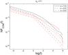 |
Fig. 20 NFCOM as a function of f for three cases of s (full: s = 1.5, dashed: s = 2.5, dot-dashed: s = 3.5) and for α0 = 0.1, and g2 = 103. The red lines indicate the analytical solution Eqs. (66) and (80). |
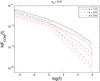 |
Fig. 21 NFCOM as a function of f for three cases of s (full: s = 1.5, dashed: s = 2.5, dot-dashed: s = 3.5) and for α0 = 0.01, and g2 = 103. The red lines indicate the analytical solution Eqs. (66) and (80). |
6.3. Numerical solution for a small injection parameter
Before we proceed with α0 ≫ 1, we want to compare the analytical result with a simple numerical integration, as we did for the linear and non-linear cooling, as well. For the plots we dropped the constant Fα, which means that we normalized the fluence by NFCOM = FCOM/Fα.
In the following plots we fix α0, and, thus,
q0 is not a free parameter any more, but becomes
 (85)This
confirms what we discussed in Sect. 2.3, that
q0 strongly influences which type of cooling occurs. The
results shown in Figs. 20 and 21 do not match each other as well as they did in the linear and
non-linear cooling cases. Although we inserted no offset, the analytical solution has a
smaller magnitude than the numerical result.
(85)This
confirms what we discussed in Sect. 2.3, that
q0 strongly influences which type of cooling occurs. The
results shown in Figs. 20 and 21 do not match each other as well as they did in the linear and
non-linear cooling cases. Although we inserted no offset, the analytical solution has a
smaller magnitude than the numerical result.
For frequencies below unity one can see, however, that the behavior of the analytical and
numerical solutions are the same. Both show a power-law with a spectral index of
ϑ1 = 1/2. For frequencies above unity and
for s > 2 the results also agree rather well, and
show the cut-off at .
For s < 2 the results do not match each other so
well any more. The numerical result cannot be represented as a single power-law, but
steepens gradually until it reaches a small plateau (which one could call a small pile-up)
at about  , and cuts off at
. This behavior is more
obvious for α0 closer to unity, which could be a hint that the
approximations are not valid enough for this case. Interestingly, for
s = 1.5 and α0 = 0.1 the analytical solution
is not continuous at , which
is a little bit strange, since it should be continuous as one can easily verify.
, and cuts off at
. This behavior is more
obvious for α0 closer to unity, which could be a hint that the
approximations are not valid enough for this case. Interestingly, for
s = 1.5 and α0 = 0.1 the analytical solution
is not continuous at , which
is a little bit strange, since it should be continuous as one can easily verify.
6.4. Large injection parameter, large spectral index
We will continue our analytical calculation of the synchrotron fluence with the case of α0 ≫ 1, and begin with s > 3.
For 0 < Ψ < Ψ2 the calculation
is the same as for α0 ≪ 1, which means that we can use the
results obtained during the calculation of that case. Thus, ![Mathematical equation: \begin{eqnarray} \Fc(1/4<f<1)=\Fa \frac{f^{-1/2}}{\gamma_1(K_0+U_0)(s-1)} \nonumber \\ \times \left[ 1-\left( f^{-1/2}-1 \right)^{s-1} \right], \label{fs3a10a1} \end{eqnarray}](/articles/aa/full_html/2010/16/aa15284-10/aa15284-10-eq266.png) (86)and
(86)and
![Mathematical equation: \begin{eqnarray} \Fc(1<f<g_2^2)=\Fa \frac{f^{-s/2}}{\gamma_1(K_0+U_0)(s-1)} \nonumber \\ \times \left[ 1-\left( \frac{f}{g_2^2} \right)^{\frac{s-1}{2}} \right]. \label{fs3a10a2} \end{eqnarray}](/articles/aa/full_html/2010/16/aa15284-10/aa15284-10-eq267.png) (87)The
next integration will be done for Ψ2 ≤ Ψ ≤ Ψ3, where
Ψ3 = f1/2α0.
Hence, the differential becomes
(87)The
next integration will be done for Ψ2 ≤ Ψ ≤ Ψ3, where
Ψ3 = f1/2α0.
Hence, the differential becomes  , and the fluence reads
 ![Mathematical equation: \begin{eqnarray} \label{fs3a10b} \Fc(f)&=&\Fa\frac{f^{-\frac{2+s}{2}}}{\alpha_0^2\gamma_1K_0}\intl_{\Psi_2}^{\Psi_3}\td{\Psi}\Psi^2(1-\Psi)^{s-2} \nonumber \\ &\quad \times & \HSF{(1-f^{1/2}g_2^{-1})-\Psi}\HSF{\Psi-(1-f^{1/2})} \nonumber \\ &=&\Fa\frac{f^{-\frac{2+s}{2}}}{\alpha_0^2\gamma_1K_0} \left[ -\frac{\Psi^2}{s-1}(1-\Psi)^{s-1} \right. \nonumber \\ &\quad -& \left.\frac{2\Psi}{s^2-s}(1-\Psi)^s-\frac{2}{s^3-s}(1-\Psi)^{s+1} \right]_a^b \nonumber \\ &\quad \approx& \Fa\frac{f^{-\frac{2+s}{2}}}{\alpha_0^2\gamma_1K_0} \left[ -\frac{\Psi^2}{s-1}(1-\Psi)^{s-1} \right]_a^b. \end{eqnarray}](/articles/aa/full_html/2010/16/aa15284-10/aa15284-10-eq271.png) (88)In
the last step we used the leading term approximation again, which we have already used
during the calculations of the non-linear fluence. We infer from the limits and the
Heaviside functions that the fluence of this part could contain three frequency regimes.
(88)In
the last step we used the leading term approximation again, which we have already used
during the calculations of the non-linear fluence. We infer from the limits and the
Heaviside functions that the fluence of this part could contain three frequency regimes.
The first one is for  , and with
a = 1 − f1/2 and
, and with
a = 1 − f1/2 and
 we
obtain
we
obtain ![Mathematical equation: \begin{eqnarray} \label{fs3a10b1} \Fc(f<\alpha_0^{-2}) &=& \Fa\frac{f^{-3/2}}{\alpha_0^2\gamma_1K_0(s-1)} \nonumber \\ &\quad \times& \left[ (1-f^{1/2})^2-f\alpha_0^2(f^{-1/2}-\alpha_0)^{s-1} \right]. \end{eqnarray}](/articles/aa/full_html/2010/16/aa15284-10/aa15284-10-eq274.png) (89)Inspecting
this solution a little further one finds that this does not contribute to the overall
fluence for
f < (α0 + 1)-2.
This means that this solution has only a very narrow regime of applicability. Therefore,
we neglect it entirely.
(89)Inspecting
this solution a little further one finds that this does not contribute to the overall
fluence for
f < (α0 + 1)-2.
This means that this solution has only a very narrow regime of applicability. Therefore,
we neglect it entirely.
The second frequency interval is  with the limits
a = 1 − f1/2, and
. Hence,
with the limits
a = 1 − f1/2, and
. Hence,
![Mathematical equation: \begin{eqnarray} \label{fs3a10b2} \Fc(\alpha_0^{-2}<f<1/4) &=& \Fa \frac{f^{-3/2}}{\alpha_0^2\gamma_1K_0(s-1)} \nonumber \\ &\quad \times& \left[ \left( 1-f^{1/2} \right)^2-\left( 1-\left( \frac{f}{g_2^2} \right)^{1/2} \right)^2 g_2^{1-s} \right] \nonumber \\ &\quad \approx& \Fa \frac{f^{-3/2}}{\alpha_0^2\gamma_1K_0(s-1)} \left[ 1-g_2^{1-s} \right]. \end{eqnarray}](/articles/aa/full_html/2010/16/aa15284-10/aa15284-10-eq277.png) (90)The
last interval is for f > 1/4,
and with a = f1/2 and
we find
(90)The
last interval is for f > 1/4,
and with a = f1/2 and
we find
![Mathematical equation: \begin{eqnarray} \label{fs3a10b3} \Fc(f>1/4) &=& \Fa \frac{f^{-\frac{2+s}{2}}}{\alpha_0^2\gamma_1K_0(s-1)} \nonumber \\ &\quad \times& \left[ f \left( 1-f^{1/2} \right)^{s-1} - \left( 1- \left( \frac{f}{g_2^2} \right)^{1/2} \right)^2 f^{\frac{s-1}{2}} g_2^{1-s} \right] \nonumber \\ &\quad \approx& \Fa \frac{f^{-s/2}}{\alpha_0^2\gamma_1K_0(s-1)} \left[ 1-f^{1/2} \right]^{s-1}. \end{eqnarray}](/articles/aa/full_html/2010/16/aa15284-10/aa15284-10-eq278.png) (91)This
solution turns negative for f > 1.
(91)This
solution turns negative for f > 1.
One integration remains, which is for Ψ > Ψ3. The
differential is substituted by
dΨ = f1/2γ1K0dy.
Thus, ![Mathematical equation: \begin{eqnarray} \label{fs3a10c} \Fc(f)&=&\Fa\frac{f^{-s/2}}{\gamma_1K_0}\intl_{\Psi_3}^{\infty}\td{\Psi}(1-\Psi)^{s-2} \nonumber \\ &\quad \times& \HSF{(1-f^{1/2}g_2^{-1})-\Psi}\HSF{\Psi-(1-f^{1/2})} \nonumber \\ &=&\Fa\frac{f^{-s/2}}{\gamma_1K_0(s-1)} \left[ -(1-\Psi) \right]_a^b\cdot \end{eqnarray}](/articles/aa/full_html/2010/16/aa15284-10/aa15284-10-eq280.png) (92)For
the limits
become a = 1 − f1/2 and
, and,
therefore,
(92)For
the limits
become a = 1 − f1/2 and
, and,
therefore, ![Mathematical equation: \begin{eqnarray} \Fc(f<\alpha_0^{-2}) = \Fa \frac{f^{-1/2}}{\gamma_1K_0(s-1)} \left[ 1-g_2^{1-s} \right]. \label{fs3a10c1} \end{eqnarray}](/articles/aa/full_html/2010/16/aa15284-10/aa15284-10-eq281.png) (93)In
the case
(93)In
the case  a = f1/2α0,
and resulting
in
a = f1/2α0,
and resulting
in ![Mathematical equation: \begin{eqnarray} \label{fs3a10c2} \Fc(f>\alpha_0^{-2}) &=& \Fa \frac{f^{-s/2}}{\gamma_1K_0(s-1)} \nonumber \\ &\quad \times& \left[ \left( 1-f^{1/2}\alpha_0 \right)^{s-1} - f^{\frac{s-1}{2}}g_2^{1-s} \right], \end{eqnarray}](/articles/aa/full_html/2010/16/aa15284-10/aa15284-10-eq284.png) (94)which
is always negative, and does not contribute to the fluence.
(94)which
is always negative, and does not contribute to the fluence.
Collecting terms the fluence for s > 3 and
α0 ≫ 1 becomes ![Mathematical equation: \begin{eqnarray} \label{fs3a10sol} \Fc(s>3,\alpha_0\gg 1) &=& \Fa \left[ \Fs{1}(f<\alpha_0^{-2}) \right. \nonumber \\ &\quad +& \Fs{2}(\alpha_0^{-2}<f<1/4)\nonumber\\ &\quad +&\Fs{3}(1/4<f<1) \nonumber \\ &\quad +& \left.\Fs{4}(1<f<g_2^2) \right], \end{eqnarray}](/articles/aa/full_html/2010/16/aa15284-10/aa15284-10-eq285.png) (95)with
(95)with
![Mathematical equation: \begin{eqnarray} \Fs{1} &=& \frac{f^{-1/2}}{\gamma_1K_0(s-1)} \left[ 1-g_2^{1-s} \right] \\ \Fs{2} &=& \frac{f^{-3/2}}{\alpha_0^2\gamma_1K_0(s-1)} \left[ 1-g_2^{1-s} \right] \\ \Fs{3} &=& \frac{f^{-1/2}}{\gamma_1(s-1)}\left[ \frac{K_0+U_0\left( f^{-1/2}-1 \right)^{s-1}}{(K_0+U_0)K_0} \right] \\ \Fs{4} &=& \frac{f^{-s/2}}{\gamma_1(K_0+U_0)(s-1)} \left[ 1-\left( \frac{f}{g_2^2} \right)^{\frac{s-1}{2}} \right] \, . \end{eqnarray}](/articles/aa/full_html/2010/16/aa15284-10/aa15284-10-eq286.png) What
we have found is a spectrum that is represented by mainly three power-laws, instead of two
as in the previous (especially the linear and non-linear) cases. For very low frequency
the spectral index is again ϑ1 = 1/2,
identically to the linear cooling, as expected. For intermediate frequency up to
f ≈ 1 the spectral index becomes
ϑ2 = 3/2, which is also expected since
this is identical to the non-linearly cooled case. In the region around unity the spectrum
changes its spectral index according to
Δϑ2 = (s − 3)/2. The
spectrum is cut off at .
What
we have found is a spectrum that is represented by mainly three power-laws, instead of two
as in the previous (especially the linear and non-linear) cases. For very low frequency
the spectral index is again ϑ1 = 1/2,
identically to the linear cooling, as expected. For intermediate frequency up to
f ≈ 1 the spectral index becomes
ϑ2 = 3/2, which is also expected since
this is identical to the non-linearly cooled case. In the region around unity the spectrum
changes its spectral index according to
Δϑ2 = (s − 3)/2. The
spectrum is cut off at .
6.5. Large injection parameter, small spectral index
Finally, we deal with the case 1 < s < 3 and α0 ≫ 1.
For  we can use the result obtained
in Sect. 6.2, yielding
we can use the result obtained
in Sect. 6.2, yielding ![Mathematical equation: \begin{eqnarray} \label{f1s3a10a1} \Fc(1<f<1/4g_2^2) &=& \Fa\frac{f^{-s/2}}{\gamma_1(K_0+U_1g_2^{3-s})(s-1)} \nonumber \\ &\quad \times& \left[ 1-\left( 1-\left( \frac{f}{g_2^2} \right)^{1/2} \right)^{s-1} \right], \end{eqnarray}](/articles/aa/full_html/2010/16/aa15284-10/aa15284-10-eq289.png) (100)and
(100)and
![Mathematical equation: \begin{eqnarray} \label{f1s3a10a2} \Fc(1/4g_2^2<f<g_2^2) &=& \Fa \frac{f^{-s/2}}{\gamma_1(K_0+U_1g_2^{3-s})(s-1)}\nonumber \\ &\quad \times& \left[ 1-\left( \frac{f}{g_2^2} \right)^{\frac{s-1}{2}} \right]\cdot \end{eqnarray}](/articles/aa/full_html/2010/16/aa15284-10/aa15284-10-eq290.png) (101)For
(101)For
 with
with  , we substitute the
derivative with
, we substitute the
derivative with  (102)resulting
in
(102)resulting
in  (103)The
integral can be expressed in terms of the hypergeometric function, but, unfortunately, one
cannot obtain an analytical form. Hence, we have to terminate further discussions of this
case.
(103)The
integral can be expressed in terms of the hypergeometric function, but, unfortunately, one
cannot obtain an analytical form. Hence, we have to terminate further discussions of this
case.
The next time step is  , where
Ψ4 ≈ f1/2α0.
Thus, the differential becomes , and the fluence reads
, where
Ψ4 ≈ f1/2α0.
Thus, the differential becomes , and the fluence reads ![Mathematical equation: \begin{eqnarray} \label{f1s3a10c} \Fc(f)&=&\Fa\frac{f^{-\frac{2+s}{2}}}{\alpha_0^2\gamma_1K_0}\intl_{\Psis_3}^{\Psis_4}\td{\Psi}\Psi^2(1-\Psi)^{s-2} \nonumber \\ &\quad \times & \HSF{(1-f^{1/2}g_2^{-1})-\Psi}\HSF{\Psi-(1-f^{1/2})} \nonumber \\ & = & \Fa\frac{f^{-\frac{2+s}{2}}}{\alpha_0^2\gamma_1K_0} \left[ -\frac{\Psi^2}{s-1}(1-\Psi)^{s-1} \right. \nonumber \\ &\quad -& \left. \frac{2\Psi}{s^2-s}(1-\Psi)^s-\frac{2}{s^3-s}(1-\Psi)^{s+1} \right]_a^b \nonumber \\ &\quad \approx & \Fa\frac{f^{-\frac{2+s}{2}}}{\alpha_0^2\gamma_1K_0} \left[ -\frac{\Psi^2}{s-1}(1-\Psi)^{s-1} \right]_a^b. \end{eqnarray}](/articles/aa/full_html/2010/16/aa15284-10/aa15284-10-eq297.png) (104)This
is identical to Eq. (88) and we used the
same approximations, again, as in that calculation. Therefore, the final results will be
the same, as well, and we can just copy them from Eqs. (90) and (91),
neglecting Eq. (89) as before:
(104)This
is identical to Eq. (88) and we used the
same approximations, again, as in that calculation. Therefore, the final results will be
the same, as well, and we can just copy them from Eqs. (90) and (91),
neglecting Eq. (89) as before:
![Mathematical equation: \begin{eqnarray} \label{f1s3a10c2}\Fc(\alpha_0^{-2}<f<1/4) &=& \Fa \frac{f^{-3/2}}{\alpha_0^2\gamma_1K_0(s-1)} \nonumber \\ &\quad \times& \left[ \left( 1-f^{1/2} \right)^2-\left( 1-\left( \frac{f}{g_2^2} \right)^{1/2} \right)^2 g_2^{1-s} \right] \nonumber \\ &\quad \approx& \Fa \frac{f^{-3/2}}{\alpha_0^2\gamma_1K_0(s-1)} \left[ 1-g_2^{1-s} \right], \end{eqnarray}](/articles/aa/full_html/2010/16/aa15284-10/aa15284-10-eq298.png) (105)and
(105)and
![Mathematical equation: \begin{eqnarray} \label{f1s3a10c3} \Fc(f>1/4) &=& \Fa \frac{f^{-\frac{2+s}{2}}}{\alpha_0^2\gamma_1K_0(s-1)} \nonumber \\ &\quad \times& \left[ f \left( 1-f^{1/2} \right)^{s-1} - \left( 1- \left( \frac{f}{g_2^2} \right)^{1/2} \right)^2 f^{\frac{s-1}{2}} g_2^{1-s} \right] \nonumber \\ &\quad \approx& \Fa \frac{f^{-s/2}}{\alpha_0^2\gamma_1K_0(s-1)} \left[ 1-f^{1/2} \right]^{s-1}\cdot \end{eqnarray}](/articles/aa/full_html/2010/16/aa15284-10/aa15284-10-eq299.png) (106)This
solution turns negative for f > 1.
(106)This
solution turns negative for f > 1.
The last integration is for  with the differential
dΨ = f1/2γ1K0dy.
Thus,
with the differential
dΨ = f1/2γ1K0dy.
Thus, ![Mathematical equation: \begin{eqnarray} \label{f1s3a10d} \Fc(f)&=&\Fa\frac{f^{-s/2}}{\gamma_1K_0}\intl_{\Psis_4}^{\infty}\td{\Psi}(1-\Psi)^{s-2} \nonumber \\ &\quad \times& \HSF{(1-f^{1/2}g_2^{-1})-\Psi}\HSF{\Psi-(1-f^{1/2})} \nonumber \\ &=&\Fa\frac{f^{-s/2}}{\gamma_1K_0(s-1)} \left[ -(1-\Psi) \right]_a^b\cdot \end{eqnarray}](/articles/aa/full_html/2010/16/aa15284-10/aa15284-10-eq301.png) (107)We
can use the solution (93) from the case
s > 3, yielding
(107)We
can use the solution (93) from the case
s > 3, yielding ![Mathematical equation: \begin{eqnarray} \label{f1s3a10d1} \Fc(f<\alpha_0^{-2}) = \Fa \frac{f^{-1/2}}{\gamma_1K_0(s-1)} \left[ 1-g_2^{1-s} \right] \, . \end{eqnarray}](/articles/aa/full_html/2010/16/aa15284-10/aa15284-10-eq302.png) (108)Since
the result of Eq. (94) is always negative,
we neglect it here, too.
(108)Since
the result of Eq. (94) is always negative,
we neglect it here, too.
Collecting terms we find ![Mathematical equation: \begin{eqnarray} \label{f1s3a10sol}\Fc(1<s<3,\alpha_0\gg 1) &=& \Fa \left[ \Fs{5}(f<\alpha_0^{-2}) \right. \nonumber \\ &\quad +& \left. \Fs{6}(\alpha_0^{-2}<f<1/4)\right.\nonumber\\ &\quad +& \left. \Fs{7}(1/4g_2^2<f<g_2^2) \right], \end{eqnarray}](/articles/aa/full_html/2010/16/aa15284-10/aa15284-10-eq303.png) (109)with
(109)with
![Mathematical equation: \begin{eqnarray} \Fs{5} &=& \frac{f^{-1/2}}{\gamma_1K_0(s-1)} \left[ 1-g_2^{1-s} \right] \\ \Fs{6} &=& \frac{f^{-3/2}}{\alpha_0^2\gamma_1K_0(s-1)} \left[ 1-g_2^{1-s} \right] \\ \Fs{7} &=& \frac{f^{-s/2}}{\gamma_1(K_0+U_1g_2^{3-s})(s-1)} \left[ 1-\left( \frac{f}{g_2^2} \right)^{\frac{s-1}{2}} \right] \, . \end{eqnarray}](/articles/aa/full_html/2010/16/aa15284-10/aa15284-10-eq304.png) Since
the frequency regime
Since
the frequency regime  is influenced by the solution
of the part , for which we could not find
an analytical expression, we neglected the solutions in the overall result of the fluence
(Eq. (109)).
is influenced by the solution
of the part , for which we could not find
an analytical expression, we neglected the solutions in the overall result of the fluence
(Eq. (109)).
Nonetheless, the obtained result is noteworthy. As a matter of fact, it is remarkably
similar to the case with s > 3 and
α0 ≫ 1. The fluence of Eq. (109) is also represented by a broken power-law, with two different but
constant spectral indices ϑ1 = 1/2 and
ϑ2 = 3/2 for frequencies below unity,
indicating that the non-linear cooling is replaced by the linear cooling for very late
times (and, hence, small frequencies). The spectrum is cut off at
, similar to every calculated
case before.
6.6. Numerical solution for a large injection parameter
As we did for α0 ≪ 1, we want to compare our analytical result for α0 ≫ 1 with a simple numerical calculation. For the plots we dropped the constant Fα, which means that we normalized the fluence by NFCOM = FCOM/Fα.
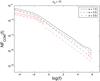 |
Fig. 22 NFCOM as a function of f for three cases of s (full: s = 1.5, dashed: s = 2.5, dot-dashed: s = 3.5) and for α0 = 10, and g2 = 103. The red lines indicate the analytical solution Eqs. (95) and (109), but with an offset of 10-4. |
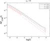 |
Fig. 23 NFCOM as a function of f for three cases of s (full: s = 1.5, dashed: s = 2.5, dot-dashed: s = 3.5) and for α0 = 100, and g2 = 103. The red lines indicate the analytical solution Eqs. (95) and (109), but with an offset of 10-4. |
 , where the
power-law breaks from the linear to the non-linear cooling, is visible in the numerical
and the analytical plots. However, in the numerical plot the spectral index for
is a little
higher than 1/2.
, where the
power-law breaks from the linear to the non-linear cooling, is visible in the numerical
and the analytical plots. However, in the numerical plot the spectral index for
is a little
higher than 1/2.
For f > 1 and s > 2 the numerical plots seem to follow an f − s/2 dependence, and one should note especially that for s = 2.5 the plot is not as steep for f > 1 as for f < 1. This is expected, when we assume that the spectral index changes at f = 1 like Δϑ2 = (s − 3)/2.
For s < 2 the curve shows a similar behavior as
in the case α0 ≪ 1, steepening gradually for
f > 1, although the steepening is not as
obvious as in the other case (cf. Sect. 6.3). One
should also note the small pile-up for s = 1.5 shortly before the
cut-off, which occurs at in all cases.
At last we should note that the results of Sect. 6 match those of SBM, at least for f < 1. This is reasonable, since the power-law electron distribution quenches rather rapidly until it becomes a δ-function, which was used by SBM.
7. Discussion and conclusions
In this paper we have made further progress in the work on nonlinear cooling of highly relativistic electrons, as it could take place in jets of active galactic nuclei. We used the nonlinear approach of RS, who introduced a cooling scenario based upon the synchrotron self-Compton effect. We expanded that paper by using a power-law for the initial electron distribution instead of a δ-function. Most of the other assumptions of the structure of the source have been unchanged, and we used the simple but rather successful model of a spherical, uniform, and nonthermal source.
We treated both the linear and the nonlinear cooling case, and calculated the respective electron number densities in Sect. 2, which differed by a new time variable that entered the nonlinear solution. We showed that the nonlinear solution cools much faster for harder spectra than for softer ones. The linear solution also cooled rather rapidly. We discussed in Sect. 2.3 that it depends critically on the choice of some parameters, which cooling acts quicker. This implies that the approach treating the cooling scenarios separately is not necessarily fulfilled, because at one moment in time the linear cooling will always dominate over the nonlinear case.
Therefore, we applied the electron distribution to a cooling scenario, which combines the linear and non-linear approach in one term. This was also already calculated for a δ-distribution of electrons by SBM. We calculated the electron number density in Sect. 3, and discussed that depending on the injection parameter α0 the electron number density showed characteristics of linear or non-linear cooling. However, even if the cooling is non-linear in the beginning, it becomes linear at later times, just as we expected.
In order to present observable quantities, we calculated analytically the emerging synchrotron intensity spectrum for all cases, and integrated them with respect to time yielding the synchrotron fluence spectrum. We began with the linear and non-linear cases in Sects. 4 and 5, respectively. In both cases the low-frequency regime of the fluence spectrum (f < 1) does not depend on the injection spectral index s of the electrons.
The fluence spectral index is ϑSYN = 1/2 for linear, and ϑSSC = 3/2 for nonlinear cooling, respectively. These constant spectral indices match those of the δ-function approach for the electron number density used by RS. This is reasonable, since we showed in Sect. 2.3 that the electron distribution becomes a δ-function for late times, when the electrons have cooled significantly and the radiated synchrotron photon energy is low.
For linear as well as for nonlinear cooling the spectra are cut off at
. In the region
 the spectral index is
s/2 with the exception of the nonlinear case with
small spectral indices, where the spectral index remains basically unchanged from the
low-energetic part.
the spectral index is
s/2 with the exception of the nonlinear case with
small spectral indices, where the spectral index remains basically unchanged from the
low-energetic part.
Section 6 was devoted to the calculation of the total
synchrotron fluence of combined cooled electrons. The results are in some ways similar to
the cases before. For α0 ≪ 1, which represents some kind of a
linear solution, the fluence shows linear characteristics. Especially, below
f = 1 the spectral index is
ϑ1 = ϑSYN = 1/2.
For α0 ≫ 1, the fluence below f = 1 exhibits a
power-law with a spectral index
ϑ2 = ϑSSC = 3/2,
just as one would expect from a non-linear cooling. However, since the non-linear cooling
becomes linear at later times, for frequencies below  the spectral index becomes
ϑ1 = ϑSYN = 1/2,
again.
the spectral index becomes
ϑ1 = ϑSYN = 1/2,
again.
Our results prove that the spectral behavior of the total synchrotron fluences in the non-linear SSC and combined synchrotron-SSC cooling cases is practically independent from the functional form of the energy injection spectrum. The earlier predictions of SBM, based on a mono-energetic injection distribution functions of electrons, on the synchrotron fluence behavior therefore hold in this case.
Online material
Appendix A: Calculation of the non-linear electron number density
Inserting the nonlinear cooling rate Eq. (6) and the injection rate into Eq. (2) gives us the differential equation for the SSC cooled electron number
density nSSC (we drop the subscript in the following):
![Mathematical equation: \appendix \setcounter{section}{1} \begin{eqnarray} \label{nleldispde1} \frac{\pd{n(\gamma,t)}}{\pd{t}} - \frac{\pd}{\pd{\gamma}}\left( A_0\gamma^2\left[\intl_{0}^{\infty}\td{\gamma}\gamma^2 n(\gamma,t)\right] n(\gamma,t) \right) = \nonumber \\ q_0\gamma^{-s}\HSF{\gamma-\gamma_1}\HSF{\gamma_2-\gamma}\DELF{t}. \end{eqnarray}](/articles/aa/full_html/2010/16/aa15284-10/aa15284-10-eq318.png) (A.1)Multiplying
the equation with
γ2/A0 we
obtain with the definitions
y = A0t and
S = γ2n
(A.1)Multiplying
the equation with
γ2/A0 we
obtain with the definitions
y = A0t and
S = γ2n![Mathematical equation: \appendix \setcounter{section}{1} \begin{eqnarray} \label{nleldispde2} \frac{\pd{S}}{\pd{y}}&-&\left[ \intl_0^{\infty}\td{\gamma}S \right]\gamma^2\frac{\pd{S}}{\pd{\gamma}} \nonumber \\ &=&q_0\gamma^{2-s} \DELF{y} \HSF{\gamma_2-\gamma}\HSF{\gamma-\gamma_1} \, . \end{eqnarray}](/articles/aa/full_html/2010/16/aa15284-10/aa15284-10-eq321.png) (A.2)We
yield with ξ = γ-1
(A.2)We
yield with ξ = γ-1![Mathematical equation: \appendix \setcounter{section}{1} \begin{eqnarray} \label{nleldispde3} \frac{\pd{S}}{\pd{y}}&\quad+&\left[ \intl_0^{\infty}\td{\xi} \frac{S}{\xi^2} \right] \frac{\pd{S}}{\pd{\xi}} \nonumber \\ &=&q_0\xi^{s-2}\DELF{y}\HSF{\xi- \xi_2}\HSF{\xi_1-\xi}\, . \end{eqnarray}](/articles/aa/full_html/2010/16/aa15284-10/aa15284-10-eq323.png) (A.3)If
we define the implicit time variable T through
(A.3)If
we define the implicit time variable T through  (A.4)the
differential equation becomes
(A.4)the
differential equation becomes 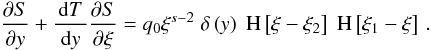 (A.5)Formally
multiplying this equation with dy ! dT results in
(A.5)Formally
multiplying this equation with dy ! dT results in
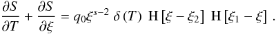 (A.6)This
differential equation for the electron number density can be solved with the method of
characteristics. Thus, we obtain
(A.6)This
differential equation for the electron number density can be solved with the method of
characteristics. Thus, we obtain 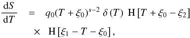 (A.7)where
ξ0 = ξ − T is a constant
of integration. Equation (A.7) can be
easily integrated with respect to T, which results in
(A.7)where
ξ0 = ξ − T is a constant
of integration. Equation (A.7) can be
easily integrated with respect to T, which results in 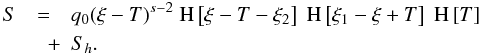 (A.8)We
now require that S(ξ = 0,T) = 0,
which means
(A.8)We
now require that S(ξ = 0,T) = 0,
which means  (A.9)Collecting
terms, we find S to be
(A.9)Collecting
terms, we find S to be 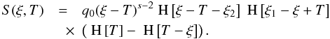 (A.10)Since
our flare begins at T = 0, we are not interested in events that take
place before that moment. Hence, we find the electron number density:
(A.10)Since
our flare begins at T = 0, we are not interested in events that take
place before that moment. Hence, we find the electron number density: 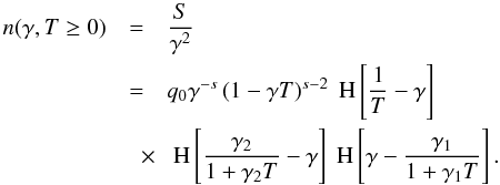 (A.11)We
see that we have two Heaviside functions defining upper limits for γ.
It is an easy task to compare them, and to find out which one is lower than the other
one. Having done so, we find the solution for the nonlinearly cooled electron number
density to be
(A.11)We
see that we have two Heaviside functions defining upper limits for γ.
It is an easy task to compare them, and to find out which one is lower than the other
one. Having done so, we find the solution for the nonlinearly cooled electron number
density to be 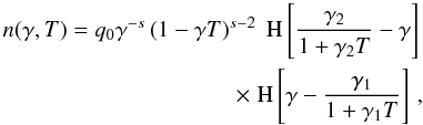 (A.12)yielding
Eq. (7).
(A.12)yielding
Eq. (7).
Appendix B: Derivation of U
The time variable T has been
defined through Eq. (8): 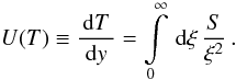 (B.1) Inserting
Eq. (A.10), we gain
(B.1) Inserting
Eq. (A.10), we gain
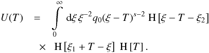 (B.2) As
stated before, we are only interested in solutions for
T ≥ 0. Hence, we can neglect the third Heaviside
function, which results in
(B.2) As
stated before, we are only interested in solutions for
T ≥ 0. Hence, we can neglect the third Heaviside
function, which results in 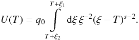 (B.3)A first substitution
w = ξ − T yields
(B.3)A first substitution
w = ξ − T yields
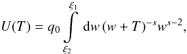 (B.4)while a second substitution w = Tv gives
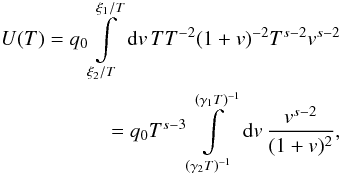 (B.5) where
we re-substituted
(B.5) where
we re-substituted  in
the last step.
in
the last step.
The purpose of the next two substitutions is to get rid of the
time variable in the limits of the integral. In order to achieve this we first set
x = γ1T
and introduce
g2 = γ2/γ1,
which yields 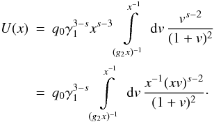 (B.6) Now,
we use u = vx, resulting in
(B.6) Now,
we use u = vx, resulting in
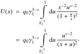 (B.7)This
integral can be expressed in terms of the hypergeometric function, but that would not
yield an analytical form. Nonetheless, one can obtain an approximate solution in the
regimes
(B.7)This
integral can be expressed in terms of the hypergeometric function, but that would not
yield an analytical form. Nonetheless, one can obtain an approximate solution in the
regimes  (small x), and
x ≥ 1 (large x).
An analytical continuation serves as a solution for the intermediate regime. For small
x the integral can be written as
(small x), and
x ≥ 1 (large x).
An analytical continuation serves as a solution for the intermediate regime. For small
x the integral can be written as
![Mathematical equation: \appendix \setcounter{section}{2} \begin{eqnarray} \label{impltimesolsmall} U_1 &=& q_0\gamma_1^{3-s}\intl_{g_2^{-1}}^{1}\td{u}\frac{u^{s-2}}{(x+u)^2} \nonumber \\ &\quad \approx& q_0\gamma_1^{3-s}\intl_{g_2^{-1}}^{1}\td{u}u^{s-4} \nonumber \\ &=& \frac{q_0\gamma_1^{3-s}}{s-3}\left[ 1-g_2^{3-s} \right]\cdot \end{eqnarray}](/articles/aa/full_html/2010/16/aa15284-10/aa15284-10-eq354.png) (B.8) Similarly,
we achieve for large x
(B.8) Similarly,
we achieve for large x ![Mathematical equation: \appendix \setcounter{section}{2} \begin{eqnarray} \label{impltimesollarge} U_3 &=& q_0\gamma_1^{3-s}\intl_{g_2^{-1}}^{1}\td{u}\frac{u^{s-2}}{(x+u)^2} \nonumber \\ &\quad \approx& q_0\gamma_1^{3-s}\intl_{g_2^{-1}}^{1}\td{u}\frac{u^{s-2}}{x^2} \nonumber \\ &=& \frac{q_0\gamma_1^{3-s}}{(s-1)x^2} \left[ 1-g_2^{1-s} \right]\cdot \end{eqnarray}](/articles/aa/full_html/2010/16/aa15284-10/aa15284-10-eq355.png) (B.9)
The requirement for the solution of the intermediate regime is that it must be continuous,
meaning
(B.9)
The requirement for the solution of the intermediate regime is that it must be continuous,
meaning  , and
U2(1) = U3(1).
In order to accomplish such a behavior, we can first assume a proper
solution U2 with some unspecified
constants, and then try to fit it to the boundary conditions. A good ansatz is
, and
U2(1) = U3(1).
In order to accomplish such a behavior, we can first assume a proper
solution U2 with some unspecified
constants, and then try to fit it to the boundary conditions. A good ansatz is
![Mathematical equation: \appendix \setcounter{section}{2} \begin{eqnarray} U_2 = \frac{q_0\gamma_1^{3-s}}{s-3}\left[ a'-b'x^{s-3}-c'\frac{g_2^{1-s}}{x^2} \right]. \label{impltimesolinte1} \end{eqnarray}](/articles/aa/full_html/2010/16/aa15284-10/aa15284-10-eq359.png) (B.10)Matching
the solution with the boundary conditions, yields the values of the constants
a′,
b′, and
c′:
(B.10)Matching
the solution with the boundary conditions, yields the values of the constants
a′,
b′, and
c′:
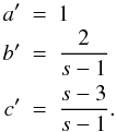 Since
we had only two equations for three parameters, we chose
a′ = 1.
Since
we had only two equations for three parameters, we chose
a′ = 1.
Thus, the obtained solution for the intermediate
x-range is ![Mathematical equation: \appendix \setcounter{section}{2} \begin{eqnarray} U_2 = \frac{q_0\gamma_1^{3-s}}{s-3}\left[ 1-\frac{2x^{s-3}}{s-1}-\frac{s-3}{s-1}\frac{g_2^{1-s}}{x^2} \right]. \label{impltimesolinte} \end{eqnarray}](/articles/aa/full_html/2010/16/aa15284-10/aa15284-10-eq365.png) (B.11)Before
we summarize the results, we need to say a few words about the spectral index
s. We already stated that it must be greater than
1. But according to our results above, we also find that
s ≠ 3. Thus, we have two different cases to
consider: s > 3, and
1 < s < 3.
(B.11)Before
we summarize the results, we need to say a few words about the spectral index
s. We already stated that it must be greater than
1. But according to our results above, we also find that
s ≠ 3. Thus, we have two different cases to
consider: s > 3, and
1 < s < 3.
Collecting terms, we find for
s > 3 ![Mathematical equation: \appendix \setcounter{section}{2} \begin{eqnarray} \label{impltimesol1app}U(x) &=& \left\{ \begin{array}{ll} U_0 \left[ 1-g_2^{3-s} \right], \quad 0\leq x\leq g_2^{-1} \\ U_0 \left[ 1-\frac{2x^{s-3}}{s-1}-\frac{s-3}{s-1}\frac{g_2^{1-s}}{x^2} \right], \quad g_2^{-1}\leq x\leq 1 \\ U_0 \frac{s-3}{(s-1)x^2}\left[ 1-g_2^{1-s} \right],\quad x\geq 1, \end{array} \right. \end{eqnarray}](/articles/aa/full_html/2010/16/aa15284-10/aa15284-10-eq368.png) (B.12)and for
1 < s < 3
(B.12)and for
1 < s < 3 ![Mathematical equation: \appendix \setcounter{section}{2} \begin{eqnarray} \label{impltimesol2app}U(x) = \left\{ \begin{array}{ll} U_1 \left[ g_2^{3-s}-1 \right], \quad 0\leq x\leq g_2^{-1} \\ U_1 \left[ \frac{2x^{s-3}}{s-1}-1-\frac{s-3}{s-1}\frac{g_2^{1-s}}{x^2} \right], \quad g_2^{-1}\leq x\leq 1 \\ U_1 \frac{3-s}{(s-1)x^2}\left[ 1-g_2^{1-s} \right], \quad x\geq 1, \end{array} \right. \end{eqnarray}](/articles/aa/full_html/2010/16/aa15284-10/aa15284-10-eq369.png) (B.13)with ,
and
(B.13)with ,
and  .
.
Appendix C: The non-linear time variable x
Since
 , we can separate the variables obtaining
 . This can be integrated quite easily except for both intermediate cases.
However, we can find approximative solutions by using the same approximations of these
cases we used already during the calculation of the synchrotron spectra.
. This can be integrated quite easily except for both intermediate cases.
However, we can find approximative solutions by using the same approximations of these
cases we used already during the calculation of the synchrotron spectra.
Beginning with the case
s > 3 we yield
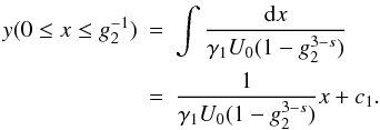 (C.1)We
require y(x = 0) = 0, which means
c1 = 0. The intermediate range becomes
(C.1)We
require y(x = 0) = 0, which means
c1 = 0. The intermediate range becomes
 (C.2)
(C.2)
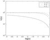 |
Fig. C.1 The denominator U(x) of the intermediate time regime as a function of x for three cases of s. |
 (C.3)These
equations can be inverted simply, yielding
x(y). As for
U(x), we
require x to be continuous at the points
(C.3)These
equations can be inverted simply, yielding
x(y). As for
U(x), we
require x to be continuous at the points
 and
y2 = y(x = 1).
Matching the solutions at these points we find the values
and
y2 = y(x = 1).
Matching the solutions at these points we find the values
![Mathematical equation: \appendix \setcounter{section}{3} \begin{eqnarray} y_1 &=& \frac{1}{\gamma_1 U_0} \frac{g_2^{-1}}{1-g_2^{3-s}} \\ y_2 &=& \frac{1}{\gamma_1 U_0} \left[ 1+\frac{g_2^{2-s}}{1-g_2^{3-s}} \right] \\ c_2 &=& \frac{1}{\gamma_1 U_0} \frac{g_2^{2-s}}{1-g_2^{3-s}} \\ c_3 &=& \frac{1}{\gamma_1 U_0} \left[ 1+\frac{g_2^{2-s}}{1-g_2^{3-s}}-\frac{s-1}{3(3-s)(1-g_2^{1-s})} \right]\cdot \end{eqnarray}](/articles/aa/full_html/2010/16/aa15284-10/aa15284-10-eq380.png) For
the case
1 < s < 3
we find similarly
For
the case
1 < s < 3
we find similarly  (C.8)We
require y(x = 0) = 0 again, which
means c4 = 0. The intermediate range
becomes
(C.8)We
require y(x = 0) = 0 again, which
means c4 = 0. The intermediate range
becomes  (C.9)
(C.9)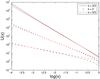 |
Fig. C.2 The denominator U(x) (black) and its leading term (red) of the intermediate time regime as a function of x for three cases of s. |
We approximated the denominator with the leading term. The validity of this approximation for most parts of the x-range can be seen in Fig. C.2 . The largest errors occur for small values of x.
The last case yields  (C.10)As
before, a simple inversion leads to
x(y), while the requirement that
the solution should be continuous at the points
(C.10)As
before, a simple inversion leads to
x(y), while the requirement that
the solution should be continuous at the points  and
y4 = y(x = 1)
gives the values
and
y4 = y(x = 1)
gives the values ![Mathematical equation: \appendix \setcounter{section}{3} \begin{eqnarray} y_3 &=& \frac{1}{\gamma_1 U_1} \frac{g_2^{-1}}{g_2^{3-s}-1} \\ y_4 &=& \frac{1}{\gamma_1 U_1} \left[ \frac{s-1}{2(4-s)}(1-g_2^{s-4})+\frac{g_2^{-1}}{g_2^{3-s}-1} \right] \\ c_5 &=& \frac{1}{\gamma_1 U_1} \left[ \frac{g_2^{-1}}{g_2^{3-s}-1}-\frac{s-1}{2(4-s)g_2^{4-s}} \right] \\ c_6 &=& \frac{1}{\gamma_1 U_1} \left[ \frac{s-1}{2(4-s)}(1-g_2^{s-4})+\frac{g_2^{-1}}{g_2^{3-s}-1} \right. \nonumber \\ &\quad - & \left.\frac{s-1}{3(3-s)(1-g_2^{1-s})} \right] \, . \end{eqnarray}](/articles/aa/full_html/2010/16/aa15284-10/aa15284-10-eq387.png)
Appendix D:
The implicit time variable
of the combined cooling
The differential Eq. (2) may look a little bit more complicated with the combined
cooling term (13).
However, the solution can be obtained with the methods outlined in
Appendix A,
yielding solution (14). The important difference is the definition of the implicit time
variable, which has to be chosen as  (D.1)Using
the definition of U from Appendix B, this can be written as
(D.1)Using
the definition of U from Appendix B, this can be written as
 (D.2)Thus,
we can use the previous results to obtain for
s > 3
(D.2)Thus,
we can use the previous results to obtain for
s > 3 ![Mathematical equation: \appendix \setcounter{section}{4} \begin{eqnarray} \label{app:implussol1}\Us(\xc,s>3) = \left\{ \begin{array}{ll} K_0+U_0 \left[ 1-g_2^{3-s} \right], \quad 0\leq \xc\leq g_2^{-1} \\ K_0+U_0, \quad g_2^{-1}\leq \xc\leq 1 \\ K_0+U_0 \frac{s-3}{(s-1)\xc^2}\left[ 1-g_2^{1-s} \right], \quad \xc\geq 1, \end{array} \right. \end{eqnarray}](/articles/aa/full_html/2010/16/aa15284-10/aa15284-10-eq392.png) (D.3)and
for
1 < s < 3
(D.3)and
for
1 < s < 3 ![Mathematical equation: \appendix \setcounter{section}{4} \begin{eqnarray} \label{app:implussol2}\Us(\xc,1<s<3) = \nonumber \\ \left\{ \begin{array}{ll} K_0+U_1 \left[ g_2^{3-s}-1 \right], \quad 0\leq \xc\leq g_2^{-1} \\ K_0+U_1 \frac{2\xc^{s-3}}{s-1}, \quad g_2^{-1}\leq \xc\leq 1 \\ K_0+U_1 \frac{3-s}{(s-1)\xc^2}\left[ 1-g_2^{1-s} \right], \quad \xc\geq 1, \end{array} \right. \end{eqnarray}](/articles/aa/full_html/2010/16/aa15284-10/aa15284-10-eq393.png) (D.4)where
we defined , and used the leading term
approximation discussed in Appendix C for the intermediate regimes.
(D.4)where
we defined , and used the leading term
approximation discussed in Appendix C for the intermediate regimes.
D.1. Large spectral index
Similarly to the steps in Appendix C, we calculate the
dependence . We begin
with the case s > 3. For
 we find
  (D.5)As
before, we set
(D.5)As
before, we set  , since
 . Inverting Eq. (D.5) yields
 (D.6)Obviously,
 is found from the condition
  yielding
  (D.7)For
 we find
  (D.8)or
the other way around
(D.8)or
the other way around  (D.9)Since is
supposed to be continuous, we find the constant
(D.9)Since is
supposed to be continuous, we find the constant  by matching the solutions for
  resulting in
 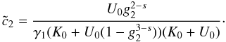 (D.10)We
also obtain
(D.10)We
also obtain  from the condition
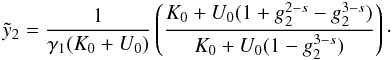 (D.11)Defining
  we yield for

![Mathematical equation: \appendix \setcounter{section}{4} \begin{eqnarray} \label{ys3a} y(\xc\geq 1)&=&\frac{1}{\gamma_1}\int\frac{\td{\xc}}{K_0+B_0\xc^{-2}} \nonumber \\ &=& \frac{1}{\gamma_1K_0}\int\td{\xc}\frac{\xc^2}{\frac{B_0}{K_0}+\xc^2} \nonumber \\ &=& \frac{1}{\gamma_1K_0}\left[ \xc-\sqrt{\frac{B_0}{K_0}}\arctan\left( \sqrt{\frac{K_0}{B_0}}\xc \right)+\cc_3 \right]. \end{eqnarray}](/articles/aa/full_html/2010/16/aa15284-10/aa15284-10-eq413.png) (D.12)The
problem arising is that we cannot find an inverted expression
for .
However, we can obtain approximative results for small and large arguments of the
arctan-function.
(D.12)The
problem arising is that we cannot find an inverted expression
for .
However, we can obtain approximative results for small and large arguments of the
arctan-function.
In order to achieve these approximations we define the
injection parameter  (D.13)for
which Eq. (D.12)
becomes
(D.13)for
which Eq. (D.12)
becomes ![Mathematical equation: \appendix \setcounter{section}{4} \begin{eqnarray} y(\xc\geq 1)=\frac{1}{\gamma_1K_0}\left[ \xc-\alpha_0\arctan\left( \frac{\xc}{\alpha_0} \right)+\cc_3 \right], \label{ys3aA} \end{eqnarray}](/articles/aa/full_html/2010/16/aa15284-10/aa15284-10-eq416.png) (D.14)For
α0 ≪ 1 the argument of the
arctan-function is always (much) larger than unity, since
(D.14)For
α0 ≪ 1 the argument of the
arctan-function is always (much) larger than unity, since
 . We, therefore, approximate
 , set
, set
 , and obtain
 ![Mathematical equation: \appendix \setcounter{section}{4} \begin{eqnarray} y(\xc\geq 1,\alpha_0\ll 1)=\frac{1}{\gamma_1K_0}\left[ \xc+\cc_3' \right]. \label{ys3a01} \end{eqnarray}](/articles/aa/full_html/2010/16/aa15284-10/aa15284-10-eq420.png) (D.15)This
can be easily inverted, yielding the linear solution
(D.15)This
can be easily inverted, yielding the linear solution  (D.16)Matching
this solution with Eq. (D.9) yields
(D.16)Matching
this solution with Eq. (D.9) yields 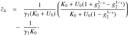 (D.17)For
α0 ≫ 1 we have to consider two cases.
If
(D.17)For
α0 ≫ 1 we have to consider two cases.
If  , we see that
 . Thus, we can approximate the
arctan-function to third order as
. Thus, we can approximate the
arctan-function to third order as
 , resulting in
![Mathematical equation: \appendix \setcounter{section}{4} \begin{eqnarray} \label{yas3a10} y(1\leq\xc\leq\alpha_0,\alpha_0 \gg 1) \nonumber \\ \approx \frac{1}{\gamma_1K_0} \left[ \xc-\alpha_0 \left( \frac{\xc}{\alpha_0} - \frac{\xc^3}{3\alpha_0^3} \right) + \cc_3 \right] \nonumber \\ = \frac{1}{\gamma_1K_0} \left[ \frac{\xc^3}{3\alpha_0^2}+\cc_3 \right]. \end{eqnarray}](/articles/aa/full_html/2010/16/aa15284-10/aa15284-10-eq426.png) (D.18)Inverting
yields
(D.18)Inverting
yields ![Mathematical equation: \appendix \setcounter{section}{4} \begin{eqnarray} \xc(\yc_2\leq y\leq\yc_3,\alpha_0\gg 1)=\left[ 3\alpha_0^2\gamma_1K_0(y-\cc_5) \right]^{1/3}, \label{xcas3a10} \end{eqnarray}](/articles/aa/full_html/2010/16/aa15284-10/aa15284-10-eq427.png) (D.19)with
(D.19)with
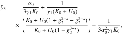 (D.20)and
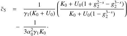 (D.21)In
the case
(D.21)In
the case  , we can approximate again
arctan(x/α0) ≈ π/2,
yielding with
, we can approximate again
arctan(x/α0) ≈ π/2,
yielding with 
![Mathematical equation: \appendix \setcounter{section}{4} \begin{eqnarray} y(\xc\geq\alpha_0,\alpha_0\gg 1)\approx\frac{1}{\gamma_1K_0}\left[ \xc+\cc_3'' \right], \label{ys3a10} \end{eqnarray}](/articles/aa/full_html/2010/16/aa15284-10/aa15284-10-eq433.png) (D.22)or
inverted
(D.22)or
inverted  (D.23)with
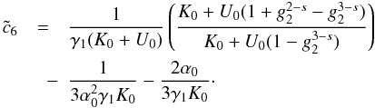 (D.24)What
one can see here is that the injection parameter controls significantly the cooling
behavior of the electrons. For α0 ≪ 1
the solution is purely linear, while for
α0 ≫ 1 it is non-linear and becomes
linear at later times, just as we expected.
(D.24)What
one can see here is that the injection parameter controls significantly the cooling
behavior of the electrons. For α0 ≪ 1
the solution is purely linear, while for
α0 ≫ 1 it is non-linear and becomes
linear at later times, just as we expected.
Before we proceed with the case
1 < s < 3
we list the results of this section once more in a compact form. We also approximate
the results for g2 ≫ 1, which, as one
will see, simplifies a lot. ![Mathematical equation: \appendix \setcounter{section}{4} \begin{eqnarray} \xc(y\leq\yc_1)&\approx& \gamma_1 (K_0+U_0) y \\ \xc(\yc_1\leq y\leq\yc_2) &\quad =& \gamma_1 (K_0+U_0) (y-\cc_2) \\ \xc(y\geq\yc_2,\alpha_0\ll 1) &\quad =& \gamma_l K_0 (y-\cc_4) \\ \xc(\yc_2\leq y\leq\yc_3,\alpha_0\gg 1) &\quad =& \left[ 3\alpha_0^2\gamma_1K_0(y-\cc_5) \right]^{1/3} \\ \xc(y\geq\yc_3,\alpha_0\gg 1) &\quad =& \gamma_1K_0(y-\cc_6), \end{eqnarray}](/articles/aa/full_html/2010/16/aa15284-10/aa15284-10-eq436.png) with
with
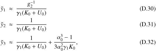 and
and
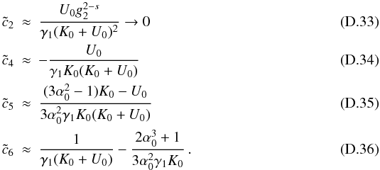 Since
in this approximation
Since
in this approximation  ,
,  , and, thus, one can neglect
.
, and, thus, one can neglect
.
D.2. Small spectral index
We will now derive the explicit form of the implicit time
variable for
1 < s < 3.
The first regime is  ,
yielding
,
yielding  (D.37)Since , obviously
d1 = 0, and the inversion becomes
(D.37)Since , obviously
d1 = 0, and the inversion becomes
 (D.38)with
 (D.39)The
next time step is
(D.39)The
next time step is  , resulting in
 (D.40)where
we defined . For
α0 ≪ 1 we see that
(D.40)where
we defined . For
α0 ≪ 1 we see that
 (as long as
s is not too close to 1
or 3), and with
(as long as
s is not too close to 1
or 3), and with  we approximate the integral as
 (D.41)The
inversion is easily performed, yielding
(D.41)The
inversion is easily performed, yielding  (D.42)where
we obtain by matching the solutions
(D.42)where
we obtain by matching the solutions  (D.43)and
 (D.44)For
α0 ≫ 1 we see that
(D.44)For
α0 ≫ 1 we see that
 . As a rough
approximation this is also much lower than ,
and, therefore, we achieve the integral
. As a rough
approximation this is also much lower than ,
and, therefore, we achieve the integral  (D.45)The
inverted equation is
(D.45)The
inverted equation is ![Mathematical equation: \appendix \setcounter{section}{4} \begin{eqnarray} \xc(\ys_1\leq y\leq\ys_3,\alpha_0\gg 1) = \left[ \frac{2\gamma_1U_1(4-s)}{s-1}(y-d_3) \right]^{\frac{1}{4-s}}, \label{xc11sa10} \end{eqnarray}](/articles/aa/full_html/2010/16/aa15284-10/aa15284-10-eq456.png) (D.46)with
(D.46)with
 (D.47)and
 (D.48)Similarly
to the case for large spectral indices, we
obtain here for the integral in that time regime
(D.48)Similarly
to the case for large spectral indices, we
obtain here for the integral in that time regime ![Mathematical equation: \appendix \setcounter{section}{4} \begin{eqnarray} \label{y1sa}y(\xc\geq 1)&=&\frac{1}{\gamma_1K_0}\int\frac{\xc^2\td{\xc}}{\alpha_0^2+\xc^2} \nonumber \\ &=&\frac{1}{\gamma_1K_0}\left[ \xc-\alpha_0\arctan\left( \frac{\xc}{\alpha_0} \right)+d_4 \right]. \end{eqnarray}](/articles/aa/full_html/2010/16/aa15284-10/aa15284-10-eq459.png) (D.49)We
will continue with the same approximations as before, yielding for
α0 ≪ 1
(D.49)We
will continue with the same approximations as before, yielding for
α0 ≪ 1  , and with
 the result
  (D.50)The
inversion is obviously
(D.50)The
inversion is obviously  (D.51)where
 (D.52)For
α0 ≫ 1 we use for
the approximation
(D.52)For
α0 ≫ 1 we use for
the approximation  , yielding
![Mathematical equation: \appendix \setcounter{section}{4} \begin{eqnarray} y(1\leq\xc\leq\alpha_0,\alpha_0\gg 1)\approx \frac{1}{\gamma_1K_0}\left[ \frac{\xc^3}{3\alpha_0^2}+d_4'' \right]. \label{ya1sa10} \end{eqnarray}](/articles/aa/full_html/2010/16/aa15284-10/aa15284-10-eq467.png) (D.53)Hence,
(D.53)Hence,
![Mathematical equation: \appendix \setcounter{section}{4} \begin{eqnarray} \xc(\ys_3\leq y\leq\ys_4,\alpha_0\gg 1)=\left[ 3\gamma_1K_0\alpha_0^2(y-d_6) \right]^{1/3}, \label{xca1sa10} \end{eqnarray}](/articles/aa/full_html/2010/16/aa15284-10/aa15284-10-eq468.png) (D.54)with
(D.54)with
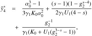 (D.55)and
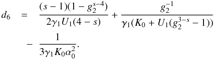 (D.56)
The last case is for , where we can use the
“linear” approximation
arctan(x/α0) ≈ π/2,
again. With  we achieve
 ![Mathematical equation: \appendix \setcounter{section}{4} \begin{eqnarray} y(\xc\geq\alpha_0,\alpha_0\gg 1)\approx \frac{1}{\gamma_1K_0}\left[ \xc+d_4''' \right], \label{y1sa10} \end{eqnarray}](/articles/aa/full_html/2010/16/aa15284-10/aa15284-10-eq472.png) (D.57)or
inverted
(D.57)or
inverted  (D.58)where
we defined
(D.58)where
we defined 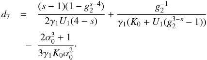 (D.59)As
we did for the case of large spectral indices, we sum up our results in a short
list, and perform the approximation for
g2 ≫ 1.
(D.59)As
we did for the case of large spectral indices, we sum up our results in a short
list, and perform the approximation for
g2 ≫ 1.
![Mathematical equation: \appendix \setcounter{section}{4} \begin{eqnarray} \xc(y\leq\ys_1) &\approx& \gamma_1(K_0+U_1g_2^{3-s})y \\ \xc(\ys_1\leq y\leq\ys_2,\alpha_0\ll 1) &=& \frac{2\gamma_1U_1\beta}{(s-1)\alpha_0^2}(y-d_2) \\ \xc(y\geq\ys_2,\alpha_0\ll 1) &=& \gamma_1K_0(y-d_5) \\ \xc(\ys_1\leq y\leq\ys_3,\alpha_0\gg 1) &=& \left[ \frac{2\gamma_1U_1(4-s)}{s-1}(y-d_3) \right]^{\frac{1}{4-s}} \\ \xc(\ys_3\leq y\leq\ys_4,\alpha_0\gg 1) &=& \left[ 3\gamma_1K_0\alpha_0^2(y-d_6) \right]^{1/3} \\ \xc(y\geq\ys_4,\alpha_0\gg 1) &=& \gamma_1K_0(y-d_7), \end{eqnarray}](/articles/aa/full_html/2010/16/aa15284-10/aa15284-10-eq475.png) with
with
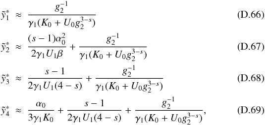 and
and
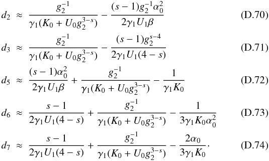
Acknowledgments
We thank the anonymous referee for his/her constructive comments which helped improving the manuscript. We acknowledge support from the German Ministry for Education and Research (BMBF) through Verbundforschung Astroteilchenphysik grant 05A08PC1 and the Deutsche Forschungsgemeinschaft through grants Schl 201/20-1 and Schl 201/23-1.
References
- Abdo, A. A., Ackermann, M., Agudo, I., et al. 2010, ApJ, 716, 30 [NASA ADS] [CrossRef] [Google Scholar]
- Aharonian, F., Akhperjanian, A. G., Bazer-Bachi, A. R., et al. 2007, ApJ, 664, L71 [Google Scholar]
- Böttcher, M. 2007, Astrophys. Space Sci., 309, 95 [Google Scholar]
- Crusius, A., & Schlickeiser, R. 1988, A&A, 196, 327 [NASA ADS] [Google Scholar]
- Dermer, C. D., & Schlickeiser, R. 1993, ApJ, 416, 458 [NASA ADS] [CrossRef] [Google Scholar]
- Dermer, C. D., & Schlickeiser, R. 2002, ApJ, 575, 667 [NASA ADS] [CrossRef] [Google Scholar]
- Eichmann, B., Schlickeiser, R., & Rhode, W. 2010, A&A, 511, A26 [NASA ADS] [CrossRef] [EDP Sciences] [Google Scholar]
- Felten, J., & Morrison, P. 1966, ApJ, 146, 686 [NASA ADS] [CrossRef] [Google Scholar]
- Ghisellini, G. 2009a, MNRAS, 399, L16 [Google Scholar]
- Ghisellini, G. 2009b, MNRAS, 399, 24 [Google Scholar]
- Ghisellini, G., Tavecchio, F., & Ghirlanda, G. 2009c, MNRAS, 399, 2041 [NASA ADS] [CrossRef] [Google Scholar]
- Kardashev, N. 1962, Sov. Astron., 6, 317 [NASA ADS] [Google Scholar]
- Meier, D. L. 2002, New Astron. Rev., 46, 247 [Google Scholar]
- Schlickeiser, R. 2009, MNRAS, 398, 1483, (RS) [NASA ADS] [CrossRef] [Google Scholar]
- Schlickeiser, R., & Lerche, I. 2007, A&A, 476, 1 [NASA ADS] [CrossRef] [EDP Sciences] [Google Scholar]
- Schlickeiser, R., & Lerche, I. 2008, A&A, 485, 315 [NASA ADS] [CrossRef] [EDP Sciences] [Google Scholar]
- Schlickeiser, R., Böttcher, M., & Menzler, U. 2010, A&A, 519, A9 (SBM) [NASA ADS] [CrossRef] [EDP Sciences] [Google Scholar]
- Spruit, H. 2010, Lect. Notes Phys. (Springer-Verlag), 794, 233 [Google Scholar]
- Venters, T., Pavlidou, V., & Reyes, L. 2009, ApJ, 703, 1939 [NASA ADS] [CrossRef] [Google Scholar]
- Zacharias, M., & Schlickeiser, R. 2009, A&A, 498, 667 [NASA ADS] [CrossRef] [EDP Sciences] [Google Scholar]
All Figures
|
Fig. 1 Linear electron distribution for s = 1.5 at four different times y for the initial values: γ1 = 101, and γ2 = 104. |
| In the text | |
|
Fig. 2 Linear electron distribution for s = 2.5 at four different times y for the initial values: γ1 = 101, and γ2 = 104. |
| In the text | |
|
Fig. 3 Linear electron distribution for s = 3.5 at four different times y for the initial values: γ1 = 101, and γ2 = 104. |
| In the text | |
|
Fig. 4 Nonlinear electron distribution for s = 1.5 at four different times y for the initial values: γ1 = 101, and γ2 = 104. |
| In the text | |
|
Fig. 5 Nonlinear electron distribution for s = 2.5 at four different times y for the initial values: γ1 = 101, and γ2 = 104. |
| In the text | |
|
Fig. 6 Nonlinear electron distribution for s = 3.5 at four different times y for the initial values: γ1 = 101, and γ2 = 104. |
| In the text | |
|
Fig. 7 Time dependence of the upper (γ2, upper curves) and lower (γ1, lower curves) cut-offs of the electron spectra, respectively, for the standard values γ1 = 101, γ2 = 104, R15 = 1, and q5 = 1. Full curve: linear electron cooling for s = 2. Dashed curve: nonlinear electron cooling for s = 2. Dotted curve: nonlinear electron cooling for s = 3.5. |
| In the text | |
|
Fig. 8 The same as in Fig. 7, but with R15 = 10, and q5 = 104. Note the different values on the horizontal axis. |
| In the text | |
|
Fig. 9 Temporal evolution of the combined electron number density for s = 1.5 and α0 = 0.1 at four different times y with the initial values γ1 = 10 and γ2 = 104. |
| In the text | |
|
Fig. 10 Temporal evolution of the combined electron number density for s = 2.5 and α0 = 0.1 at four different times y with the initial values γ1 = 10 and γ2 = 104. |
| In the text | |
|
Fig. 11 Temporal evolution of the combined electron number density for s = 3.5 and α0 = 0.1 at four different times y with the initial values γ1 = 10 and γ2 = 104. |
| In the text | |
|
Fig. 12 Temporal evolution of the combined electron number density for s = 1.5 and α0 = 100 at four different times y with the initial values γ1 = 10 and γ2 = 104. |
| In the text | |
|
Fig. 13 Temporal evolution of the combined electron number density for s = 2.5 and α0 = 100 at four different times y with the initial values γ1 = 10 and γ2 = 104. |
| In the text | |
|
Fig. 14 Temporal evolution of the combined electron number density for s = 3.5 and α0 = 100 at four different times y with the initial values γ1 = 10 and γ2 = 104. |
| In the text | |
|
Fig. 15 Temporal evolution of the cut-offs of the combined electron number density for s = 2.0 and α0 = 0.1 for the initial values γ1 = 10 and γ2 = 104. |
| In the text | |
|
Fig. 16 Temporal evolution of the cut-offs of the combined electron number density for s = 2.0 (full curve), s = 3.5 (dashed curve) and α0 = 100 for the initial values γ1 = 10 and γ2 = 104. |
| In the text | |
|
Fig. 17 NFSYN as a function of f for three cases of s (full: s = 2, dashed: s = 3, dot-dashed: s = 4) and for g2 = 103. The red lines indicate the analytical solution Eq. (29) with an offset of 10-0.7. |
| In the text | |
|
Fig. 18 NFSSC as a function of f for three cases of s > 3 full: s = 3.1, dashed: s = 4, dot-dashed: s = 5) and for g2 = 103. The red lines indicate the analytical solution Eqs. (43)–(46) with an offset of 10-0.9. |
| In the text | |
|
Fig. 19 NFSSC as a function of f for three cases of s > 3 (full: s = 3.1, dashed: s = 4, dot-dashed: s = 5) and for g2 = 103. The red lines indicate the analytical solution Eqs. (56) and (57) with an offset of 10-0.9. |
| In the text | |
|
Fig. 20 NFCOM as a function of f for three cases of s (full: s = 1.5, dashed: s = 2.5, dot-dashed: s = 3.5) and for α0 = 0.1, and g2 = 103. The red lines indicate the analytical solution Eqs. (66) and (80). |
| In the text | |
|
Fig. 21 NFCOM as a function of f for three cases of s (full: s = 1.5, dashed: s = 2.5, dot-dashed: s = 3.5) and for α0 = 0.01, and g2 = 103. The red lines indicate the analytical solution Eqs. (66) and (80). |
| In the text | |
|
Fig. 22 NFCOM as a function of f for three cases of s (full: s = 1.5, dashed: s = 2.5, dot-dashed: s = 3.5) and for α0 = 10, and g2 = 103. The red lines indicate the analytical solution Eqs. (95) and (109), but with an offset of 10-4. |
| In the text | |
|
Fig. 23 NFCOM as a function of f for three cases of s (full: s = 1.5, dashed: s = 2.5, dot-dashed: s = 3.5) and for α0 = 100, and g2 = 103. The red lines indicate the analytical solution Eqs. (95) and (109), but with an offset of 10-4. |
| In the text | |
|
Fig. C.1 The denominator U(x) of the intermediate time regime as a function of x for three cases of s. |
| In the text | |
|
Fig. C.2 The denominator U(x) (black) and its leading term (red) of the intermediate time regime as a function of x for three cases of s. |
| In the text | |
Current usage metrics show cumulative count of Article Views (full-text article views including HTML views, PDF and ePub downloads, according to the available data) and Abstracts Views on Vision4Press platform.
Data correspond to usage on the plateform after 2015. The current usage metrics is available 48-96 hours after online publication and is updated daily on week days.
Initial download of the metrics may take a while.