| Issue |
A&A
Volume 524, December 2010
|
|
|---|---|---|
| Article Number | A31 | |
| Number of page(s) | 23 | |
| Section | Astrophysical processes | |
| DOI | https://doi.org/10.1051/0004-6361/201015284 | |
| Published online | 22 November 2010 | |
Online material
Appendix A: Calculation of the non-linear electron number density
Inserting the nonlinear cooling rate Eq. (6) and the injection rate into Eq. (2) gives us the differential equation for the SSC cooled electron number
density nSSC (we drop the subscript in the following):
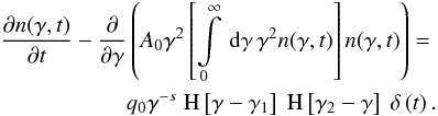 (A.1)Multiplying
the equation with
γ2/A0 we
obtain with the definitions
y = A0t and
S = γ2n
(A.1)Multiplying
the equation with
γ2/A0 we
obtain with the definitions
y = A0t and
S = γ2n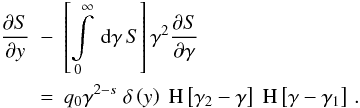 (A.2)We
yield with ξ = γ-1
(A.2)We
yield with ξ = γ-1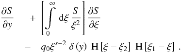 (A.3)If
we define the implicit time variable T through
(A.3)If
we define the implicit time variable T through 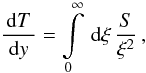 (A.4)the
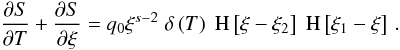
differential equation becomes
(A.4)the
differential equation becomes 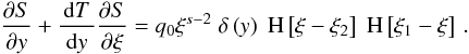 (A.5)Formally
multiplying this equation with dy ! dT results in
(A.5)Formally
multiplying this equation with dy ! dT results in
 (A.6)This
differential equation for the electron number density can be solved with the method of
characteristics. Thus, we obtain
(A.6)This
differential equation for the electron number density can be solved with the method of
characteristics. Thus, we obtain 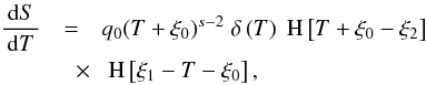 (A.7)where
ξ0 = ξ − T is a constant
of integration. Equation (A.7) can be
easily integrated with respect to T, which results in
(A.7)where
ξ0 = ξ − T is a constant
of integration. Equation (A.7) can be
easily integrated with respect to T, which results in 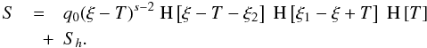 (A.8)We
now require that S(ξ = 0,T) = 0,
which means
(A.8)We
now require that S(ξ = 0,T) = 0,
which means  (A.9)Collecting
terms, we find S to be
(A.9)Collecting
terms, we find S to be 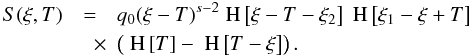 (A.10)Since
our flare begins at T = 0, we are not interested in events that take
place before that moment. Hence, we find the electron number density:
(A.10)Since
our flare begins at T = 0, we are not interested in events that take
place before that moment. Hence, we find the electron number density: 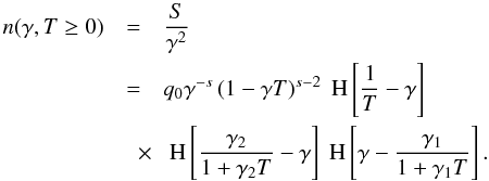 (A.11)We
see that we have two Heaviside functions defining upper limits for γ.
It is an easy task to compare them, and to find out which one is lower than the other
one. Having done so, we find the solution for the nonlinearly cooled electron number
density to be
(A.11)We
see that we have two Heaviside functions defining upper limits for γ.
It is an easy task to compare them, and to find out which one is lower than the other
one. Having done so, we find the solution for the nonlinearly cooled electron number
density to be 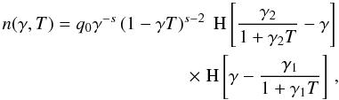 (A.12)yielding
Eq. (7).
(A.12)yielding
Eq. (7).
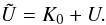
Appendix B: Derivation of U
The time variable T has been
defined through Eq. (8): 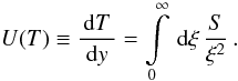 (B.1) Inserting
Eq. (A.10), we gain
(B.1) Inserting
Eq. (A.10), we gain
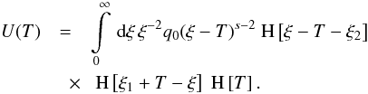 (B.2) As
stated before, we are only interested in solutions for
T ≥ 0. Hence, we can neglect the third Heaviside
function, which results in
(B.2) As
stated before, we are only interested in solutions for
T ≥ 0. Hence, we can neglect the third Heaviside
function, which results in 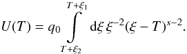 (B.3)A first substitution
w = ξ − T yields
(B.3)A first substitution
w = ξ − T yields
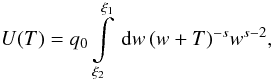 (B.4)while a second substitution w = Tv gives
 (B.5) where
we re-substituted
(B.5) where
we re-substituted  in
the last step.
in
the last step.
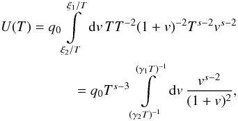
The purpose of the next two substitutions is to get rid of the
time variable in the limits of the integral. In order to achieve this we first set
x = γ1T
and introduce
g2 = γ2/γ1,
which yields 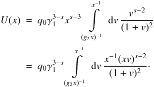 (B.6) Now,
we use u = vx, resulting in
(B.6) Now,
we use u = vx, resulting in
 (B.7)This
integral can be expressed in terms of the hypergeometric function, but that would not
yield an analytical form. Nonetheless, one can obtain an approximate solution in the
regimes
(B.7)This
integral can be expressed in terms of the hypergeometric function, but that would not
yield an analytical form. Nonetheless, one can obtain an approximate solution in the
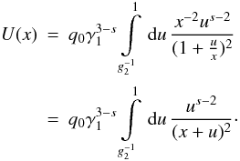
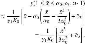
regimes  (small x), and
x ≥ 1 (large x).
An analytical continuation serves as a solution for the intermediate regime. For small
x the integral can be written as
(small x), and
x ≥ 1 (large x).
An analytical continuation serves as a solution for the intermediate regime. For small
x the integral can be written as
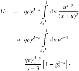 (B.8) Similarly,
we achieve for large x
(B.8) Similarly,
we achieve for large x 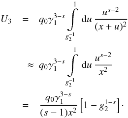 (B.9)
The requirement for the solution of the intermediate regime is that it must be continuous,
meaning
(B.9)
The requirement for the solution of the intermediate regime is that it must be continuous,
meaning  , and
U2(1) = U3(1).
In order to accomplish such a behavior, we can first assume a proper
solution U2 with some unspecified
constants, and then try to fit it to the boundary conditions. A good ansatz is
, and
U2(1) = U3(1).
In order to accomplish such a behavior, we can first assume a proper
solution U2 with some unspecified
constants, and then try to fit it to the boundary conditions. A good ansatz is
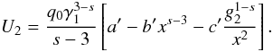 (B.10)Matching
the solution with the boundary conditions, yields the values of the constants
a′,
b′, and
c′:
(B.10)Matching
the solution with the boundary conditions, yields the values of the constants
a′,
b′, and
c′:
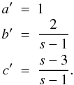 Since
we had only two equations for three parameters, we chose
a′ = 1.
Since
we had only two equations for three parameters, we chose
a′ = 1.
Thus, the obtained solution for the intermediate
x-range is 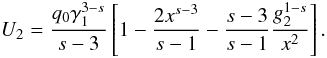 (B.11)Before
we summarize the results, we need to say a few words about the spectral index
s. We already stated that it must be greater than
1. But according to our results above, we also find that
s ≠ 3. Thus, we have two different cases to
consider: s > 3, and
1 < s < 3.
(B.11)Before
we summarize the results, we need to say a few words about the spectral index
s. We already stated that it must be greater than
1. But according to our results above, we also find that
s ≠ 3. Thus, we have two different cases to
consider: s > 3, and
1 < s < 3.
Collecting terms, we find for
s > 3 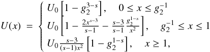 (B.12)and for
1 < s < 3
(B.12)and for
1 < s < 3 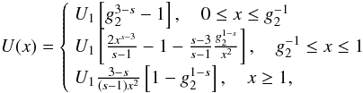 (B.13)with
  ,
and
,
and  .
.
Appendix C: The non-linear time variable x
Since
 , we can separate the variables obtaining
 . This can be integrated quite easily except for both intermediate cases.
However, we can find approximative solutions by using the same approximations of these
cases we used already during the calculation of the synchrotron spectra.
. This can be integrated quite easily except for both intermediate cases.
However, we can find approximative solutions by using the same approximations of these
cases we used already during the calculation of the synchrotron spectra.
Beginning with the case
s > 3 we yield
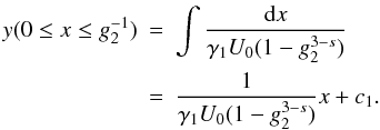 (C.1)We
require y(x = 0) = 0, which means
c1 = 0. The intermediate range becomes
(C.1)We
require y(x = 0) = 0, which means
c1 = 0. The intermediate range becomes
 (C.2)
(C.2)
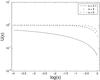 |
Fig. C.1 The denominator U(x) of the intermediate time regime as a function of x for three cases of s. |
| Open with DEXTER | |
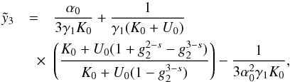
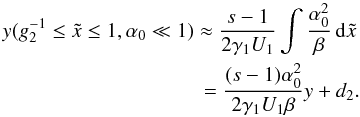
 (C.3)These
equations can be inverted simply, yielding
x(y). As for
U(x), we
require x to be continuous at the points
(C.3)These
equations can be inverted simply, yielding
x(y). As for
U(x), we
require x to be continuous at the points
 and
y2 = y(x = 1).
Matching the solutions at these points we find the values
and
y2 = y(x = 1).
Matching the solutions at these points we find the values
 For
the case
1 < s < 3
we find similarly
For
the case
1 < s < 3
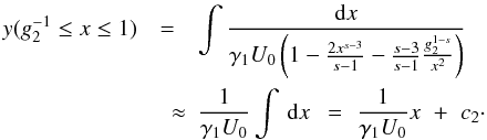
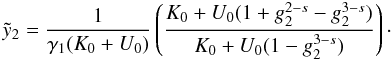
we find similarly  (C.8)We
require y(x = 0) = 0 again, which
means c4 = 0. The intermediate range
becomes
(C.8)We
require y(x = 0) = 0 again, which
means c4 = 0. The intermediate range
becomes  (C.9)
(C.9)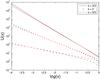 |
Fig. C.2 The denominator U(x) (black) and its leading term (red) of the intermediate time regime as a function of x for three cases of s. |
| Open with DEXTER | |
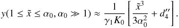
We approximated the denominator with the leading term. The validity of this approximation for most parts of the x-range can be seen in Fig. C.2 . The largest errors occur for small values of x.
The last case yields  (C.10)As
before, a simple inversion leads to
x(y), while the requirement that
the solution should be continuous at the points
(C.10)As
before, a simple inversion leads to
x(y), while the requirement that
the solution should be continuous at the points  and
y4 = y(x = 1)
gives the values
and
y4 = y(x = 1)
gives the values 
Appendix D:
The implicit time variable  of the combined cooling
The differential Eq. (2) may look a little bit more complicated with the combined
cooling term (13).
However, the solution can be obtained with the methods outlined in
Appendix A,
yielding solution (14). The important difference is the definition of the implicit time
variable, which has to be chosen as  (D.1)Using
the definition of U from Appendix B, this can be written as
(D.1)Using
the definition of U from Appendix B, this can be written as
 (D.2)Thus,
we can use the previous results to obtain for
s > 3
(D.2)Thus,
we can use the previous results to obtain for
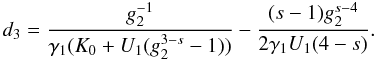
s > 3 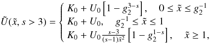 (D.3)and
for
1 < s < 3
(D.3)and
for
1 < s < 3 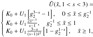 (D.4)where
we defined
(D.4)where
we defined  , and used the leading term
approximation discussed in Appendix C for the intermediate regimes.
, and used the leading term
approximation discussed in Appendix C for the intermediate regimes.
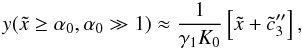
D.1. Large spectral index
Similarly to the steps in Appendix C, we calculate the
dependence  . We begin
with the case s > 3. For
. We begin
with the case s > 3. For
 we find
 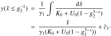 (D.5)As
before, we set
(D.5)As
before, we set  , since
 . Inverting Eq. (D.5) yields
 (D.6)Obviously,
 is found from the condition
  yielding
  (D.7)For
 we find
 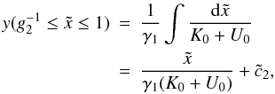 (D.8)or
the other way around
(D.8)or
the other way around  (D.9)Since is
supposed to be continuous, we find the constant
(D.9)Since is
supposed to be continuous, we find the constant  by matching the solutions for
  resulting in
 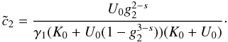 (D.10)We
also obtain
(D.10)We
also obtain  from the condition
 (D.11)Defining
 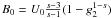 we yield for

 (D.12)The
problem arising is that we cannot find an inverted expression
for .
However, we can obtain approximative results for small and large arguments of the
arctan-function.
(D.12)The
problem arising is that we cannot find an inverted expression
for .
However, we can obtain approximative results for small and large arguments of the
arctan-function.
In order to achieve these approximations we define the
injection parameter 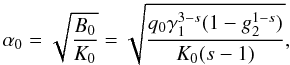 (D.13)for
which Eq. (D.12)
becomes
(D.13)for
which Eq. (D.12)
becomes 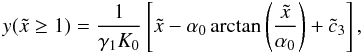 (D.14)For
α0 ≪ 1 the argument of the
arctan-function is always (much) larger than unity, since
(D.14)For
α0 ≪ 1 the argument of the
arctan-function is always (much) larger than unity, since
 . We, therefore, approximate
 , set
, set
 , and obtain
 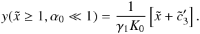 (D.15)This
can be easily inverted, yielding the linear solution
(D.15)This
can be easily inverted, yielding the linear solution  (D.16)Matching
this solution with Eq. (D.9) yields
(D.16)Matching
this solution with Eq. (D.9) yields 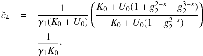 (D.17)For
α0 ≫ 1 we have to consider two cases.
If
(D.17)For
α0 ≫ 1 we have to consider two cases.
If  , we see that
 . Thus, we can approximate the
arctan-function to third order as
. Thus, we can approximate the
arctan-function to third order as
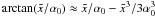 , resulting in
 (D.18)Inverting
yields
(D.18)Inverting
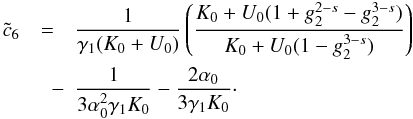
yields  (D.19)with
 (D.20)and
 (D.21)In
the case
(D.21)In
the case  , we can approximate again
arctan(x/α0) ≈ π/2,
yielding with
, we can approximate again
arctan(x/α0) ≈ π/2,
yielding with 
 (D.22)or
inverted
(D.22)or
inverted  (D.23)with
 (D.24)What
one can see here is that the injection parameter controls significantly the cooling
behavior of the electrons. For α0 ≪ 1
the solution is purely linear, while for
α0 ≫ 1 it is non-linear and becomes
linear at later times, just as we expected.
(D.24)What
one can see here is that the injection parameter controls significantly the cooling
behavior of the electrons. For α0 ≪ 1
the solution is purely linear, while for
α0 ≫ 1 it is non-linear and becomes
linear at later times, just as we expected.
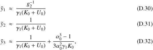
Before we proceed with the case
1 < s < 3
we list the results of this section once more in a compact form. We also approximate
the results for g2 ≫ 1, which, as one
will see, simplifies a lot. 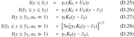 with
with
 and
and
 Since
in this approximation
Since
in this approximation  ,
,  , and, thus, one can neglect
.
, and, thus, one can neglect
.
D.2. Small spectral index
We will now derive the explicit form of the implicit time
variable for
1 < s < 3.
The first regime is  ,
yielding
,
yielding  (D.37)Since , obviously
d1 = 0, and the inversion becomes
(D.37)Since , obviously
d1 = 0, and the inversion becomes
 (D.38)with
 (D.39)The
next time step is
(D.39)The
next time step is  , resulting in
 (D.40)where
we defined
(D.40)where
we defined 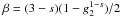 . For
α0 ≪ 1 we see that
. For
α0 ≪ 1 we see that
 (as long as
s is not too close to 1
or 3), and with
(as long as
s is not too close to 1
or 3), and with  we approximate the integral as
 (D.41)The
inversion is easily performed, yielding
(D.41)The
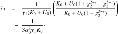
inversion is easily performed, yielding 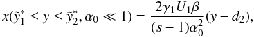 (D.42)where
we obtain by matching the solutions
(D.42)where
we obtain by matching the solutions 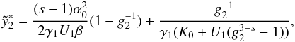 (D.43)and
 (D.44)For
α0 ≫ 1 we see that
(D.44)For
α0 ≫ 1 we see that
 . As a rough
approximation this is also much lower than
. As a rough
approximation this is also much lower than  ,
and, therefore, we achieve the integral
,
and, therefore, we achieve the integral  (D.45)The
inverted equation is
(D.45)The
inverted equation is  (D.46)with
 (D.47)and
 (D.48)Similarly
to the case for large spectral indices, we
obtain here for the integral in that time regime
(D.48)Similarly
to the case for large spectral indices, we
obtain here for the integral in that time regime 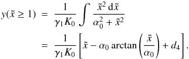 (D.49)We
will continue with the same approximations as before, yielding for
α0 ≪ 1
(D.49)We
will continue with the same approximations as before, yielding for
α0 ≪ 1  , and with
 the result
 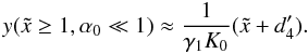 (D.50)The
inversion is obviously
(D.50)The
inversion is obviously  (D.51)where
 (D.52)For
α0 ≫ 1 we use for
the approximation
(D.52)For
α0 ≫ 1 we use for
the approximation  , yielding
 (D.53)Hence,
 (D.54)with
 (D.55)and
 (D.56)
The last case is for , where we can use the
“linear” approximation
arctan(x/α0) ≈ π/2,
again. With  we achieve
 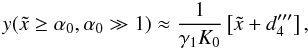 (D.57)or
inverted
(D.57)or
inverted  (D.58)where
we defined
(D.58)where
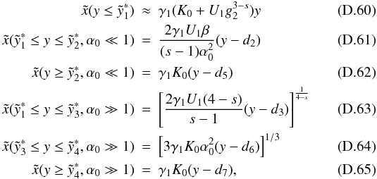
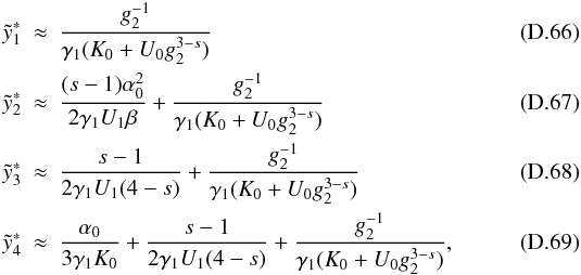
we defined 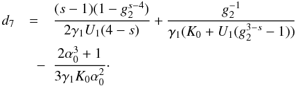 (D.59)As
we did for the case of large spectral indices, we sum up our results in a short
list, and perform the approximation for
g2 ≫ 1.
(D.59)As
we did for the case of large spectral indices, we sum up our results in a short
list, and perform the approximation for
g2 ≫ 1.
 with
with
 and
and
© ESO, 2010
Current usage metrics show cumulative count of Article Views (full-text article views including HTML views, PDF and ePub downloads, according to the available data) and Abstracts Views on Vision4Press platform.
Data correspond to usage on the plateform after 2015. The current usage metrics is available 48-96 hours after online publication and is updated daily on week days.
Initial download of the metrics may take a while.