| Issue |
A&A
Volume 524, December 2010
|
|
|---|---|---|
| Article Number | A62 | |
| Number of page(s) | 9 | |
| Section | Galactic structure, stellar clusters and populations | |
| DOI | https://doi.org/10.1051/0004-6361/201014901 | |
| Published online | 23 November 2010 | |
Calibration of radii and masses of open clusters with a simulation
1
Astronomisches Rechen-Institut, Zentrum für Astronomie der
Universität Heidelberg, Mönchhofstrasse 12–14, 69120
Heidelberg,
Germany
e-mail: aernst@ari.uni-heidelberg.de
2
National Astronomical Observatories of China, Chinese Academy of
Sciences, Datun Lu 20A, Chaoyang
District, Beijing
100012, PR
China
3
Main Astronomical Observatory, National Academy of Sciences of
Ukraine, Akademika Zabolotnoho
27, 03680
Kyiv,
Ukraine
4
Institut für Astronomie der Universität Wien,
Türkenschanzstraße
17, 1180
Wien,
Austria
Received:
30
April
2010
Accepted:
1
September
2010
Context. Piskunov and collaborators developed a method to make a simple mass estimate for tidally limited star clusters based on the identification of the tidal radius in a King profile with the dynamical Jacobi radius. The application of this method to an unbiased open cluster catalog yielded significantly higher cluster masses than the classical methods.
Aims. We quantify the bias in the mass determination as a function of projection direction and cluster age by analyzing a simulated star cluster.
Methods. We use direct N-body simulations of a star cluster in an analytic Milky Way potential that account for stellar evolution and apply a best fit to the projected number density of cluster stars.
Results. We obtain significantly overestimated star cluster masses that depend strongly on the viewing direction. The overestimation is typically in the range of 10–50 percent and reaches a factor of 3.5 for young clusters. Mass segregation reduces the derived limiting radii systematically.
Key words: methods: statistical / methods: data analaysis / open clusters and associations: general / solar neighborhood
© ESO, 2010
1. Introduction
Piskunov et al. (2007, 2008a,b) developed an approach to determining the masses of open star clusters (OCs) and applied it to determine the initial and present-day mass function of OCs in the solar neighborhood. The method is based on the determination of the tidal radius rt from the cumulative number of cluster members as a function of projected distance from the cluster center. For each cluster, the tidal radius rt is determined from projected number density profiles by fitting a King 1962 profile (King 1962). The identification of the King cutoff radius rt with the “Jacobi” radius rJ (i.e., the dynamical tidal radius, which is the distance from the cluster center to the Lagrange points L1 and L2) then yields the OC mass from the standard formula given here by Eq. (9) solved for Mcl. The application of this dynamical mass estimate for tidally limited clusters to an unbiased OC catalog yields a mass determination that is independent of the classical methods. A detailed comparison with other cluster mass determinations is also made. In a second step, the method is extended to all OCs of an unbiased cluster catalog by establishing a transformation of the observed semi-major axis and central surface density to rt. These results were then used to derive the cluster present-day mass function (CPDMF) and the initial mass function of OCs (CIMF) in the extended solar neighborhood. Adopting a constant cluster formation rate over the past 10 Gyr yields a surface density of 18M⊙pc-2 of stars born in OCs. This corresponds to a fraction of 37% of disk stars born in OCs (Röser et al. 2010). This is large compared to the classical values of the order of 10% or less (e.g., Wielen 1971; Miller & Scalo 1978).
Some crucial assumptions enter the dynamical mass determination based on fitting a King profile: a) The OC fills its Roche lobe in the tidal field of the Milky Way. For compact (e.g. Roche-lobe underfilling) clusters, rJ and as a consequence the mass can be underestimated by a large amount; b) The effect of mass segregation can be neglected, i.e., star counts on the upper main sequence, which dominate the observed cluster members, are representative of the mass distribution; c) The elliptic shape of the clusters and the contamination by tidal tail stars do not result in a systematic bias. Shape parameters were measured by Kharchenko et al. (2009) and the distribution of tidal tail stars have been investigated in detail (e.g. Just et al. 2009); d) The tidal radius rt determined by fitting the cumulative projected mass profile represents the Jacobi radius rJ used to derive the cluster mass. Since the cluster mass depends on the third power of rJ, the method is very sensitive to systematic errors in the derivation of rJ.
In the present paper, we quantify the possible bias introduced by identifying the tidal radius rt inferred from a King profile fitting with the Jacobi radius rJ used for the mass determination by Piskunov et al. (2007). We applied the King profile fitting procedure to a direct N-body simulation of a dissolving star cluster at different evolutionary states. We simulated a star cluster on a circular orbit at RC = 8.5 kpc which evolved in the tidal field of the Milky Way including stellar evolution. We took snapshots of the evolved model with all stellar masses and positions at four different times and projected the snapshots from the perspective of an observer on Earth (at R0 = 8 kpc) onto the sky, at different positions along its orbit. After all, we determined the model’s limiting radius rt by fitting the projected cumulative mass profile with Eq. (6) and compared rt to the actual Jacobi radius rJ.
The paper is organized as follows. In Sect. 2 we discuss the method of N-body simulations in the external potential of the Milky Way and Sect. 3 contains the theory of the cluster geometry in a tidal field. In Sect. 4, we show a simple iterative method to determine the Jacobi radius of an N-body model of a star cluster in a tidal field. In Sect. 5, the projection and fitting methods are described. Finally, Sect. 6 contains our results and Sect. 7 our conclusions.
2. Numerical simulation
We analyze in detail a numerical simulation of a star cluster with initial mass M0 = 104 M⊙ on a circular orbit in an analytic Milky Way potential. It is the fiducial cluster simulation (run 10) discussed in Just et al. (2009). We chose this cluster because it is representative of the high-mass end of the observed OCs. Since the total mass of the cluster system is dominated by the high-mass end, the correction of biases in the mass determination are most important in that parameter regime. The cluster was set up as a W0 = 6 King model with a half-mass radius of 8 pc. The extension of the cluster initially exceeds the Roche lobe initially leading to an enhanced mass loss in the first 0.5 Gyr. We used a Salpeter IMF and included mass loss by stellar evolution. The total lifetime of the cluster at a circular orbit with RC = 8.5 kpc is 6.3 Gyr. For details of the evolution we refer to Just et al. (2009).
In a high-resolution simulation of a dissolving star cluster with N = 40404 particles in the tidal field of the Milky Way the direct N-body code φgrape1 (Harfst et al. 2007) was used with the micro-grape6 special-purpose hardware at the Astronomisches Rechen-Institut (ARI) in Heidelberg2. φgrape is an acronym for Parallel Hermite Integration with grape. The code is written in ansi-c and uses a fourth-order Hermite scheme (Makino & Aarseth 1992) for the orbit integration. It is parallelized and uses the MPI library to communicate between the processors. The force computations are executed on the fast special-purpose hardware grape. The special-purpose micro-grape6 hardware cards are designed especially to calculate gravitational forces in N-body simulations rapidly using parallelization with pipelining (see Harfst et al. 2007, and references therein).
The code φgrape does not adopt regularization as the codes nbody4 or nbody6++ (Aarseth 1999, 2003; Spurzem 1999) do. Rather, it uses a standard Plummer type N-body gravitational softening. The softening length in the model used for the current work was ϵ = 10-3 pc. We tested for different softening lengths ϵ = 10-3,10-4, and 10-5 pc that there are no significant differences regarding shape evolution and star-cluster mass loss.
For the simulation of a star cluster in the tidal field of the Galaxy, the N-body problem is solved in an analytic background potential. We use an axisymmetric three-component model, where the bulge, disc, and halo are described by Plummer-Kuzmin models (Miyamoto & Nagai 1975) with the potential
 (1)The parameters a,b, and M of the Milky Way model are given in Table 1 for the three components.
The top panel of Fig. 1 shows the rotation curve of the three-component model of the Milky Way. The parameters of the three-component model are chosen such that the rotation curve matches that of the Milky Way (Dauphole & Colin 1995). At the solar radius R0 = 8.0 kpc, which was assumed in this study, the value of the circular velocity is V0 = 234.2 km s-1. The values of Oort’s constants A and B are consistent with the observed values (A,B) = (14.5 ± 0.8, −13.0 ± 1.1) km s-1/kpc derived by Piskunov et al. (2006). More generally, the dimensionless epicyclic and vertical frequency parameters are given by  where κ, ν, and Ω are the epicyclic, vertical, and circular frequencies of a near-circular orbit and ρ is the local Galactic density (see Oort 1965, for the derivation of δ2). The bottom panel of Fig. 1 shows the course of the epicyclic and vertical frequency parameters β and δ.
The list of galaxy component parameters.
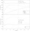 |
Fig. 1 Top: rotation curve (at z = 0) of the three-component Plummer-Kuzmin model of the Milky Way. Bottom: epicyclic and vertical frequency parameters β = κ/Ω and δ = ν/Ω (at z = 0). |
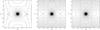 |
Fig. 2 Cut through the equipotential surfaces of Eq. (8) along the principal axis planes. The extents xmax (i.e. rJ), ymax (from Eq. (11)) and zmax (from Eq. (15)) of the last closed equipotential surface is marked with dashed lines. We assumed a Kepler potential for the cluster. |
3. Cluster geometry
According to King (1962), the projected density profile Σ(r) of a star cluster can be approximated by 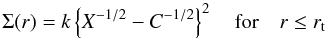 (4)with normalization constant k and
  (5)where rc is the core radius and rt is the (tidal) cutoff radius where the projected density of the model drops to zero. Integration yields the cumulative form of the King (1962) profile,
 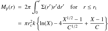 (6)where Mp(r) is the projected cumulative mass of the model, i.e. the mass in projection on the sky within a circle of radius r. For r > rt, we force the integrated profile (Eq. (6)) to the finite value
 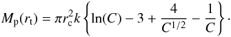 (7)We do not use the identification of Mp(rt) with the cluster mass, since in practice the equations are applied to star counts and the effective mass-of-light ratio enters the normalization constant k.
Already King (1961) remarks that the tidal forces from the galaxy distort only the outer regions of a star cluster. We quantify these deviations from spherical symmetry caused by the tidal field in this section. We employ a coordinate system (x, y, z) of “principal axes of the star cluster”. Its origin is the cluster center. The x-axis points away from the Galactic center, the y-axis points in the direction of the Galactic rotation and the z-axis is directed towards the Galactic north pole. Figure 2 shows a “principal axis plane cut” through the equipotential surfaces of the effective potential around a star cluster on a circular orbit in the tidal field of the Milky Way. To second order, the effective potential is given by 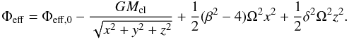 (8)For the cluster, we assumed a Kepler potential, which is a very good approximation in the outer parts (Just et al. 2009). The unit in Fig. 2 is the Jacobi radius rJ. The Jacobi radius is defined as the distance from the cluster center to the Lagrange points L1 and L2. It is given by
 ![\begin{equation} r_{\rm J} = \left[ \frac{GM_{\rm cl}}{(4-\beta^2)\Omega^2} \right]^{1/3} \label{eq:rjac} \end{equation}](/articles/aa/full_html/2010/16/aa14901-10/aa14901-10-eq64.png) (9)(see King 1962). The value of the effective potential on the critical equipotential surface, which connects L1 and L2, can be easily calculated from Eqs. (8) and (9). It is given by
(9)(see King 1962). The value of the effective potential on the critical equipotential surface, which connects L1 and L2, can be easily calculated from Eqs. (8) and (9). It is given by  (10)Assuming that xmax = rJ, the radius in the y-direction of the last closed (critical) equipotential surface follows from Eqs. (8) and (10),
  (11)For the radius in z-direction, we have to solve a cubic equation
  (12)with the constants
  (13)The only real solution is given by
 ![\begin{equation} z_{\rm max} = \frac{\left\{ K \left[K+2L \left( LM^3 + \sqrt{KM^3+L^2M^6}\right)\right]\right\}^{1/3}-K^{2/3}}{L \left(LM^3 + \sqrt{KM^3+L^2M^6}\right)^{1/3} }\cdot \end{equation}](/articles/aa/full_html/2010/16/aa14901-10/aa14901-10-eq70.png) (14)For (β,δ) = (βC,δC) = (1.37,2.86), we obtain
(14)For (β,δ) = (βC,δC) = (1.37,2.86), we obtain  (15)(e.g. Wielen 1974). More generally, the ratios of the principal axes ymaxtoxmax and zmaxtoxmax of all closed equipotential surfaces are shown in Fig. 3 as a function of the parameter γ = x/rJ. At the center of the cluster we have γ = 0, while γ = 1 corresponds to the critical equipotential surface through x = rJ.
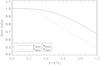 |
Fig. 3 Principal axis ratios of the equipotential surfaces around the cluster as a function of the parameter γ = x/rJ. At the center of the cluster, we have γ = 0 while γ = 1 (dashed line) corresponds to the critical equipotential surface through x = rJ. We assumed (β,δ) = (1.37,2.86) and a Kepler potential for the cluster. |
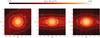 |
Fig. 4 Surface density of projections onto the principal axis planes of the cluster at T4 = 1.31 Gyr. The dashed lines show the theoretical values of xmax/rJ, ymax/rJ, and zmax/rJ. The contours correspond to Δlog Σ ≈ 2 dex. |
4. Jacobi radius of the model
We determined the Jacobi radius of our simulated N-body model iteratively from Eq. (9). The gravitational constant G and the quantities β and Ω are known but Mcl, the cluster mass within r = rJ is unknown since rJ is unknown. Our iteration is given by ![\begin{equation} r_{n+1} = \left[ \frac{GM_{\rm enc}(r_{n})}{(4-\beta^2)\Omega^2} \right]^{1/3} \label{eq:rjacit} \end{equation}](/articles/aa/full_html/2010/16/aa14901-10/aa14901-10-eq89.png) (16)where Menc(r) is the enclosed mass of cluster stars within radius r around the cluster center. Starting with r0 = ∞, the iteration theoretically converges towards r∞ = rJ. In practice, a few iterations are sufficient to determine rJ accurately. We note that this simple method does not rely on numerical fits of the effective potential to the envelope of the spatial distribution of Jacobi energies of the cluster stars. It can easily be applied to an N-body snapshot file that contains masses and positions of the individual particles at a certain time.
(16)where Menc(r) is the enclosed mass of cluster stars within radius r around the cluster center. Starting with r0 = ∞, the iteration theoretically converges towards r∞ = rJ. In practice, a few iterations are sufficient to determine rJ accurately. We note that this simple method does not rely on numerical fits of the effective potential to the envelope of the spatial distribution of Jacobi energies of the cluster stars. It can easily be applied to an N-body snapshot file that contains masses and positions of the individual particles at a certain time.
5. Projection and fitting
We calculate the projection at the sky in Galactic coordinates (l,b) and ignore for simplicity the perspective effects. Strictly speaking the projection of the cluster model is consistent only in the midplane b = 0° corresponding to the circular orbit in the Galactic plane. The rotation angle α is related to the Galactic longitude l by the law of sines 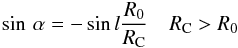 (17)where R0 = 8 kpc at the solar circle and RC = 8.5 kpc at the cluster orbit. At the Galactic coordinates (l,b) = (0,0) and (l,b) = (180°,0), the “system (x, y, z) of principal axes of the cluster” with origin at the cluster center is not rotated. We note that at l = 90° and l = 270° we have the maximum rotation angle
  and
and  , respectively.
A sketch of the projection of the simulated N-body model of the star cluster onto the plane of the sky is illustrated in Fig. 5. Four orbital positions of the dissolving star cluster with its tidal tails are marked in the sketch.
To demonstrate the effect of different projections also in Galactic latitude, we add the cases of a certain height of the cluster orbit above and below the plane of the solar circle (dotted lines in Fig. 5). The effect of the corresponding vertical oscillation of the cluster orbit on the intrinsic structure of the cluster and of a variation in δ in Eq. (2) are neglected in this study.
For all positions of the cluster on its orbit, we rotate the cluster around the z axis and then around the y′ axis by the ordered pair of angles (α, −b) to simulate the perspective of the cluster for an observer on earth. After the projection, we determine the polar symmetric profile of the projected cumulative mass Mp(r) from our N-body data file by summations over radius and polar angle and apply a fit with Eq. (6). For the fitting, we used the mpfit package in idl (Markwardt 2009; Moré 1978, for the Levenberg-Marquardt algorithm).
6. Results
We now discuss projections according to Eq. (17) in detail. Figure 6 shows examples of fits (upper panels) with the corresponding projections (lower panels). The resulting parameter ratio rt/rJ is given in the upper panels and the (l, b) coordinates in the corresponding lower panels. In the upper panels, the solid (black) line represents the data and dotted (blue) line the fit. The dashed (red) lines indicate rc (left dashed line) and rt (right dashed line) derived in the fit with Eq. (6). In the lower panels, the dashed (red) line indicates rJ.
We derived the ratio rt/rJ for all projection directions in (l,b) at four different evolution times of the cluster. The projections are performed in steps of 4 degrees from b = −90° to b = +90° and l = 0 to l = 360°. The full N-body snapshot file with N = 40404 particles has been used for the projection and fitting procedure as described in Sect. 5. Figure 7 shows parameter surfaces of rt/rJ as a function of Galactic coordinates of the cluster center at times T1 = 0.62 Gyr (top left), T2 = 0.84 Gyr (top right), T3 = 1.06 Gyr (bottom left) and T4 = 1.31 Gyr (bottom right). A squeezed Hammer-Aitoff projection of Galactic coordinates has been used (see Appendix A). The total number of fits for each plot in Fig. 7 is Nfits = 4186. We note that in the plot for T1, a peak around (l,b) ≈ (270°,0) (see also Fig. A.1 in Appendix A) is not resolved (white colored area). Here rt/rJ reaches a factor of 1.52.
It can be seen that the cluster masses are typically overestimated. The strongest bias to high masses at time T1 (including the peak) shows that the unbound stars stay for a long time close to the cluster and contribute to the outer density profile in the fitting procedure. This bias depends on the initial conditions. At later times T3, T4, the cluster mass distribution becomes stable and the bias is independent of the age of the cluster.
Figure 8 shows a histogram of the fraction on the sky per bin in Mt/Mcl = (rt/rJ)3 for the parameter surface in Fig. 7 corresponding to time T4, where the “tidal” masses Mt and Mcl are calculated with Eq. (9) from rt and rJ, respectively. The solid line shows the distribution for projections in the range −20° < b < +20°. The most frequent overestimation of the mass is Mt/Mcl = 1.18. The dashed line shows the distribution for projections in the range −40° < b < +40°. The most frequent ratio is the same as for the solid line. However, the ratios extend up to Mt/Mcl = 1.7. The dotted line shows the distribution for all projections.The most frequent ratio is the same as for the other two lines, but the ratios extend up to Mt/Mcl ≈ 2.1.
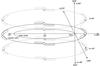 |
Fig. 5 Sketch of the Galactic coordinate system in which the projection is done. The Galactocentric radius of the Sun is assumed to be R0 = 8.0 kpc, while the cluster orbits at RC = 8.5 kpc on a circular orbit. The abbreviations denote the Galactic north (NGP) and south (SGP) Pole and the Galactic center (GC). |
Figure 9 shows the mean mass ⟨ Mt/Mcl ⟩ as a function of the Galactic latitude b, where Mt is the mass of cluster stars within radius rt derived from the fitting procedure. Shown are the curves corresponding to times T1 − T4. All curves show a local minimum located roughly at b = 0°. For time T1, the mean overestimation of the mass reaches 2.5 in the direction of the Galactic poles.
Only a small fraction of cluster stars are usually identified as members leading to an increased statistical uncertainty in the fitting procedure. The uppermost plot in Fig. 10 shows the parameter surface derived for the 400 most massive (i.e. the brightest) stars in the simulation at time T4 (data courtesy of Beuria). The small values of rt/rJ are caused by mass segregation. The stronger asymmetries with respect to b = 0° compared to the plots in Fig. 7 are due to a slightly asymmetric distribution of the 400 mass-segregated stars in position space.
In order to measure the statistical scatter in rt, we applied a bootstrap analysis. We divided the N-body snapshot file for time T4 with N = 40404 particles into 100 small-number samples of Nsample = 400 particles each (the remaining particles were dropped out of the analysis). For each of these small-number samples we applied the procedure described above. The resulting total number of projections and fits was therefore Nfits = 418600. The middle and bottom plots in Fig. 10 show the results of the bootstrap analysis. The middle plot of Fig. 10 shows the mean value of rt/rJ averaged over the 100 samples. The bottom plot shows the relative standard deviation Δrt/rt evaluated by averaging over the 100 samples. The uncertainty in a single determination of rt is between 10% and 20%. The highest uncertainty is expected for rt-determinations in the vicinity of the peak around (l,b) ≈ (270°,0).
A comparison with the uppermost plot in Fig. 10 shows that the derived limiting radii for the sample of the most massive stars are systematically lower because of mass segregation. The differences are typically on a 1 − 2σ level.
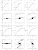 |
Fig. 6 Examples of fits (upper panels) with the corresponding projections (lower panels) at time T4 = 1.31 Gyr. The resulting parameter ratio rt/rJ is given in the upper panels and the (l, b) coordinates in the corresponding lower panels. In the upper panels, the solid (black) line represents the data and dotted (blue) line the fit. The dashed (red) lines mark rc (left dashed line) and rt (right dashed line) from the fit with Eq. (6). In the lower panels, the dashed (red) line marks rJ. |
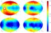 |
Fig. 7 Parameter surfaces of rt/rJ as a function of Galactic coordinates for a fit of King (1962) models to projections on the sky of a simulated model at different positions on its theoretical orbit. We used a squeezed Hammer-Aitoff projection. The color denotes the value of rt/rJ on a linear scale. The plots in the top row correspond to T1 = 0.62 Gyr (top left) and T2 = 0.84 Gyr (top right). The plots in the bottom row correspond to T3 = 1.06 Gyr (bottom left) and T4 = 1.31 Gyr (bottom right). |
7. Conclusions
In this paper, we have confirmed that star cluster masses are typically overestimated if the method of Piskunov et al. (2007) is applied to a complete sample. Moreover, we have quantified the methodological error in our analysis.
Figures 7 and 10 show that at certain Galactic coordinates the King (1962) profile fits are particularly biased. A high bias is predicted for (l,b) ≈ (270°,0) (see Figs. 7, 10, and A.1). The corresponding rotation angle of the cluster is α = 70°, where the projection is parallel to the inner end of the tidal arms (see lower left plots in Fig. 6). For (l,b) = (90°,0), there is no corresponding peak in the parameter surface (most clearly visible for T1) because of the asymmetry between the leading and trailing tidal tails (see the sketch in Fig. 5). For Galactic latitudes beyond b ≈ ±40° (cf. Fig. A.1), the bias becomes large but only a few OCs occupy this regime.
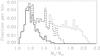 |
Fig. 8 Histogram of the fraction on the sky per bin in Mt/Mcl corresponding to the T4 = 1.31 Gyr parameter surface from Fig. 7. Mt and Mcl are the “tidal masses” calculated with Eq. (9) from rt and rJ, respectively. |
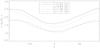 |
Fig. 9 Mean mass ⟨ Mt/Mcl ⟩ as a function of the Galactic latitude b. Mt and Mcl are the “tidal masses” calculated with Eq. (9) from rt and rJ, respectively. |
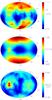 |
Fig. 10 Parameter surfaces of rt/rJ and Δrt/rt as a function of Galactic coordinates for a fit of King (1962) models to to projections on the sky of a simulated model at different positions on its theoretical orbit. We used a squeezed Hammer-Aitoff projection. The time is T4 = 1.31 Gyr. The color denotes the value of rt/rJ (and Δrt/rt, bottom plot) on a linear scale. The upper plots shows the parameter surface for the 400 brightest stars in the simulated cluster (data courtesy of Beuria). The middle and bottom plots show the result of the bootstrap analysis (for explanations see the text). The middle plot shows the mean value of rt/rJ averaged over 100 small-number samples. The bottom plot shows the corresponding relative standard deviation Δrt/rt. |
For the parameter surfaces in Fig. 7, the masses are biased within the ranges [1.3Mcl, 3.5Mcl] (at T1), [1.1Mcl, 2.3Mcl] (at T2), [1.0Mcl, 2.0Mcl] (at T3) and [1.0Mcl, 2.1Mcl] (at T4) depending on the evolutionary state of the star cluster in the tidal field of the Galaxy. The bias depends strongly on the projection angles, which transform differently into Galactic coordinates for different orbital radii of the OC.
Furthermore, we have demonstrated using a bootstrap analysis that the relative error in a single determination of the limiting radius rt is between 10% and 20% (at time T4) corresponding to an uncertainty in the mass of ≈ 50% for samples of Nsample = 400 particles (which are typical of rich OCs).
We have shown that the mass segregation of the brightest stars in a cluster can alter the rt/rJ factor significantly, which is an important result for the data analysis of observations. The mass segregation results in a concentrated core that causes an underestimation of the tidal radius. For a younger cluster age, one would expect a smaller amount of mass segregation.
To apply a quantitative correction for the bias in the cluster mass determination by identifying rt with rJ an extensive parameter study of cluster parameters is necessary. The influence of mass-segregation on selection effects caused by the brightness limit of the observations should be considered by such a study, because stellar evolution is taken into account. For young clusters, the bias factor can be particularly sensitive to the initial conditions. The final goal is to find an agreement between the OC mass determinations by the different methods. This would allow an interesting insight into the OC properties such as the IMF, mass-to-light ratio, and mass segregation.
Acknowledgments
The authors thank J. Beuria for his help with the Hammer-Aitoff projections and the provision of the data for the uppermost plot in Fig. 10. P.B. and M.I.P. acknowledge the special support by the Ukrainian National Academy of Sciences under the Main Astronomical Observatory GRAPE/GRID computing cluster project. P.B. acknowledges the support from the Volkswagen Foundation GRACE Project No. I80 041-043. M.I.P. acknowledges support by the University of Vienna through the frame of the Initiative Kolleg (IK) “The Cosmic Matter Circuit” I033-N and computing time on the Grape Cluster of the University of Vienna.
References
- Aarseth, S. J. 1999, PASP, 111, 1333 [NASA ADS] [CrossRef] [Google Scholar]
- Aarseth, S. J. 2003, Gravitational N-body simulations – Tools and Algorithms (Cambridge Univ. Press) [Google Scholar]
- Casertano, S., & Hut, P. 1985, ApJ, 298, 80 [Google Scholar]
- Dauphole, B., & Colin, J. 1995, A&A, 300, 117 [NASA ADS] [Google Scholar]
- Harfst, S., Gualandris, A., Merritt, D., et al. 2007, New Astron., 12, 357 [NASA ADS] [CrossRef] [Google Scholar]
- Just, A., Berczik, P., Petrov, M. I., & Ernst, A. 2009, MNRAS, 392, 969 [NASA ADS] [CrossRef] [Google Scholar]
- Kharchenko, N. V., Berczik, P., Petrov, M. I., et al. 2009, A&A, 495, 807 [NASA ADS] [CrossRef] [EDP Sciences] [Google Scholar]
- King, I. 1961, AJ, 66, 68 [NASA ADS] [CrossRef] [Google Scholar]
- King, I. 1962, AJ, 67, 471 [NASA ADS] [CrossRef] [Google Scholar]
- Makino, J., & Aarseth, S. J. 1992, PASJ, 44, 141 [NASA ADS] [Google Scholar]
- Markwardt, C. B. 2009, in proc. Astronomical Data Analysis Software and Systems XVIII, Quebec, Canada, ed. D. Bohlender, P. Dowler, & D. Durand, San Francisco, ASP Conf. Ser., 411, 251 [Google Scholar]
- Miller, G. E., & Scalo, J. M. 1978, PASP, 90, 506 [NASA ADS] [CrossRef] [Google Scholar]
- Miyamoto, M., & Nagai, R. 1975, PASJ, 27, 533 [NASA ADS] [Google Scholar]
- Moré, J. 1978, in Numerical Analysis, ed. G. A. Watson (Berlin: Springer Verlag), 630, 105 [Google Scholar]
- Oort, J. H. 1965, in Galactic Structure, ed. A. Blaauw, & M. Schmidt (Chicago, IL: Univ. Chicago Press), 455 [Google Scholar]
- Piskunov, A. E., Schilbach, E., Kharchenko, N. V., Röser, S., & Scholz, R.-D. 2007, A&A, 468, 151 [NASA ADS] [CrossRef] [EDP Sciences] [Google Scholar]
- Piskunov, A. E., Schilbach, E., Kharchenko, N. V., Röser, S., & Scholz, R.-D. 2008a, A&A, 477, 165 [NASA ADS] [CrossRef] [EDP Sciences] [Google Scholar]
- Piskunov, A. E., Kharchenko, N. V., Schilbach, E., et al. 2008b, A&A, 487, 557 [NASA ADS] [CrossRef] [EDP Sciences] [Google Scholar]
- Roeser, S., Kharchenko, N. V., Piskunov, A. E., et al. 2010, Astron. Nachr., 331, 519 [NASA ADS] [CrossRef] [Google Scholar]
- Spurzem, R. J. 1999, Comp. Applied Maths., 109, 407 [Google Scholar]
- Wielen, R. 1971, A&A, 13, 309 [NASA ADS] [Google Scholar]
- Wielen, R. 1974, in Proceedings of the 1st European Astronomical Meeting, Stars and the Milky Way System, ed. L. N. Mavridis (Berlin: Springer), 2, 326 [Google Scholar]
Appendix A: Squeezed Hammer-Aitoff projection
 |
Fig. A.1 Squeezed Hammer-Aitoff projection. The Galactic latitude runs from b = −90° to b = +90° and the longitude from l = 0 to l = 360°. |
The squeezed Hammer-Aitoff projection is given by 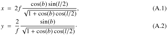 It represents the standard Hammer-Aitoff equal-area projection, where we have also introduced a free squeezing factor f. The squeezing leaves the area element
  invariant, where g is the first fundamental form calculated from Eqs. (A.1) and (A.2). The ratio of diameters of the elliptic projection area is given by dx/dy = f2. For the standard Hammer-Aitoff projection, we have
  . For a projection onto a circular area one can set f = 1. The inverse projection is given by
 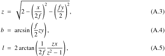 where we have introduced the auxiliary variable z.
We assumed that f = 1.2 for Figs. 7 and 10. The resulting coordinate system (which is hidden in Figs. 7 and 10) can be seen in Fig. A.1. We modified idl routines by Landsman to incorporate the free squeezing factor.
All Tables
All Figures
|
Fig. 1 Top: rotation curve (at z = 0) of the three-component Plummer-Kuzmin model of the Milky Way. Bottom: epicyclic and vertical frequency parameters β = κ/Ω and δ = ν/Ω (at z = 0). |
| In the text | |
|
Fig. 2 Cut through the equipotential surfaces of Eq. (8) along the principal axis planes. The extents xmax (i.e. rJ), ymax (from Eq. (11)) and zmax (from Eq. (15)) of the last closed equipotential surface is marked with dashed lines. We assumed a Kepler potential for the cluster. |
| In the text | |
|
Fig. 3 Principal axis ratios of the equipotential surfaces around the cluster as a function of the parameter γ = x/rJ. At the center of the cluster, we have γ = 0 while γ = 1 (dashed line) corresponds to the critical equipotential surface through x = rJ. We assumed (β,δ) = (1.37,2.86) and a Kepler potential for the cluster. |
| In the text | |
|
Fig. 4 Surface density of projections onto the principal axis planes of the cluster at T4 = 1.31 Gyr. The dashed lines show the theoretical values of xmax/rJ, ymax/rJ, and zmax/rJ. The contours correspond to Δlog Σ ≈ 2 dex. |
| In the text | |
|
Fig. 5 Sketch of the Galactic coordinate system in which the projection is done. The Galactocentric radius of the Sun is assumed to be R0 = 8.0 kpc, while the cluster orbits at RC = 8.5 kpc on a circular orbit. The abbreviations denote the Galactic north (NGP) and south (SGP) Pole and the Galactic center (GC). |
| In the text | |
|
Fig. 6 Examples of fits (upper panels) with the corresponding projections (lower panels) at time T4 = 1.31 Gyr. The resulting parameter ratio rt/rJ is given in the upper panels and the (l, b) coordinates in the corresponding lower panels. In the upper panels, the solid (black) line represents the data and dotted (blue) line the fit. The dashed (red) lines mark rc (left dashed line) and rt (right dashed line) from the fit with Eq. (6). In the lower panels, the dashed (red) line marks rJ. |
| In the text | |
|
Fig. 7 Parameter surfaces of rt/rJ as a function of Galactic coordinates for a fit of King (1962) models to projections on the sky of a simulated model at different positions on its theoretical orbit. We used a squeezed Hammer-Aitoff projection. The color denotes the value of rt/rJ on a linear scale. The plots in the top row correspond to T1 = 0.62 Gyr (top left) and T2 = 0.84 Gyr (top right). The plots in the bottom row correspond to T3 = 1.06 Gyr (bottom left) and T4 = 1.31 Gyr (bottom right). |
| In the text | |
|
Fig. 8 Histogram of the fraction on the sky per bin in Mt/Mcl corresponding to the T4 = 1.31 Gyr parameter surface from Fig. 7. Mt and Mcl are the “tidal masses” calculated with Eq. (9) from rt and rJ, respectively. |
| In the text | |
|
Fig. 9 Mean mass ⟨ Mt/Mcl ⟩ as a function of the Galactic latitude b. Mt and Mcl are the “tidal masses” calculated with Eq. (9) from rt and rJ, respectively. |
| In the text | |
|
Fig. 10 Parameter surfaces of rt/rJ and Δrt/rt as a function of Galactic coordinates for a fit of King (1962) models to to projections on the sky of a simulated model at different positions on its theoretical orbit. We used a squeezed Hammer-Aitoff projection. The time is T4 = 1.31 Gyr. The color denotes the value of rt/rJ (and Δrt/rt, bottom plot) on a linear scale. The upper plots shows the parameter surface for the 400 brightest stars in the simulated cluster (data courtesy of Beuria). The middle and bottom plots show the result of the bootstrap analysis (for explanations see the text). The middle plot shows the mean value of rt/rJ averaged over 100 small-number samples. The bottom plot shows the corresponding relative standard deviation Δrt/rt. |
| In the text | |
|
Fig. A.1 Squeezed Hammer-Aitoff projection. The Galactic latitude runs from b = −90° to b = +90° and the longitude from l = 0 to l = 360°. |
| In the text | |
Current usage metrics show cumulative count of Article Views (full-text article views including HTML views, PDF and ePub downloads, according to the available data) and Abstracts Views on Vision4Press platform.
Data correspond to usage on the plateform after 2015. The current usage metrics is available 48-96 hours after online publication and is updated daily on week days.
Initial download of the metrics may take a while.