| Issue |
A&A
Volume 524, December 2010
|
|
|---|---|---|
| Article Number | A58 | |
| Number of page(s) | 21 | |
| Section | Extragalactic astronomy | |
| DOI | https://doi.org/10.1051/0004-6361/201014733 | |
| Published online | 23 November 2010 | |
Extremely metal-poor stars in classical dwarf spheroidal galaxies: Fornax, Sculptor, and Sextans⋆
1
Laboratoire d’Astrophysique, École Polytechnique Fédérale de Lausanne
(EPFL), Observatoire, 1290
Sauverny,
Switzerland
e-mail: This email address is being protected from spambots. You need JavaScript enabled to view it.
2
GEPI, Observatoire de Paris, CNRS UMR 8111, Université Paris
Diderot, 92125
Meudon Cedex,
France
3
Department Cassiopée, University of Nice Sophia-Antipolis,
Observatoire de Côte d’Azur, CNRS, 06304
Nice Cedex 4,
France
4
McDonald Observatory, University of Texas,
Fort Davis, TX
79734,
USA
5
Kapteyn Astronomical Institute, University of
Groningen, PO Box
800, 9700AV
Groningen, The
Netherlands
6
Institute of Astronomy, University of Cambridge,
Madingley Road, Cambridge
CB3 0HA,
UK
7
European Southern Observatory, Karl-Schwarzschild-str. 2, 85748, Garching bei München,
Germany
8
Dept. of Physics & Astronomy, University of
Victoria, 3800 Finerty Road,
Victoria, BC
V8P 1A1,
Canada
9 Kavli Institute for
Particle-Astrophysics and Cosmology, Stanford University, SLAC National Accelerator
Laboratory, Menlo
Park
94025,
USA
10
European Southern Observatory, Alonso de Cordova 3107, Santiago, Chile
Received: 4 April 2010
Accepted: 19 August 2010
Abstract
We present the results of a dedicated search for extremely metal-poor stars in the Fornax, Sculptor, and Sextans dSphs. Five stars were selected from two earlier VLT/Giraffe and HET/HRS surveys and subsequently followed up at high spectroscopic resolution with VLT/UVES. All of them turned out to have [Fe/H] ≲ −3 and three stars are below [Fe/H] ~ −3.5. This constitutes the first evidence that the classical dSphs Fornax and Sextans join Sculptor in containing extremely metal-poor stars and suggests that all of the classical dSphs contain extremely metal-poor stars. One giant in Sculptor at [Fe/H] = −3.96 ± 0.06 is the most metal-poor star ever observed in an external galaxy. We carried out a detailed analysis of the chemical abundances of the α, iron peak, and the heavy elements, and we performed a comparison with the Milky Way halo and the ultra faint dwarf stellar populations. Carbon, barium, and strontium show distinct features characterized by the early stages of galaxy formation and can constrain the origin of their nucleosynthesis.
Key words: stars: abundances / Galaxy: evolution / Galaxy: stellar content / galaxies: star formation
Tables 6 and 7 are only available in electronic form at http://www.aanda.org
© ESO, 2010
1. Introduction
Extremely metal-poor stars (EMPS), with [Fe/H] < −3, are eagerly sought in the Milky Way and beyond, because they provide insight into the earliest stages of chemical enrichment processes. With only a few exceptions, the interstellar gas out of which stars form is preserved in their outer atmospheres even as they evolve up the red giant branch (RGB). High-resolution abundance analyses of RGB stars can provide detailed information about the chemical enrichment of the galaxy at the time the star was formed; this is a process we will refer to in this context as chemical tagging. Since RGB stars can have a wide range of lifetimes, depending on their mass, this allows us to build up a very accurate picture of how chemical evolution progressed with time, from the very first stars until one Gyr ago.
The most elusive stars in this chemical tagging process are the extremely metal-poor stars (EMPS), which sample the earliest epochs of chemical enrichment in a galaxy. There have been numerous detailed studies devoted to the search (e.g. Christlieb et al. 2002; Beers & Christlieb 2005) and characterization (e.g. McWilliam et al. 1995; Ryan et al. 1996; Carretta et al. 2002; Cayrel et al. 2004; Cohen et al. 2004; François et al. 2007; Lai et al. 2008; Bonifacio et al. 2009) of EMPS in the Galaxy over the last two decades. But similar studies in extra-galactic systems only became feasible with the advent of the 8−10 m class telescopes. One of the surprising results of spectroscopic studies with large telescopes of individual RGB stars in nearby dwarf spheroidal galaxies (dSphs), was the apparent lack of EMPS (e.g. Helmi et al. 2006; Aoki et al. 2009), even though the average metallicity of most of these systems is very low. However, recent results suggest that this lack of EMPS in dSphs is merely an artifact of the method used to search for them (e.g. Kirby et al. 2008; Starkenburg et al. 2010; Frebel et al. 2010a).
The overarching motivation to find and study the most primitive stars in a galaxy is the information they provide about the early chemical enrichment processes and the speed and uniformity of this environmental pollution. A key question is whether chemical enrichment progresses in the same way in dwarf galaxies as compared with larger galaxies such as the Milky Way. Probing the chemical enrichment history in different environments leads to a better understanding of which processes dominate in the early universe and for how long. It is important to separate initial processes from environmental effects, which can dominate the later development of enrichment patterns. The studies of the metal-poor population in the Galactic halo suggests that early enrichment occurs very quickly and uniformly. But it is very hard to obtain a reliable overall picture, given the large diffuse nature of the Galactic halo and the overwhelming numbers of thin and thick disk stars that mask that population. Dwarf spheroidal galaxies are much smaller environments, and it is much easier to study a significant fraction of their stellar population in a uniform way. Although dSphs have almost certainly lost stars, gas, and metals over time, most are unlikely to have gained any. It is therefore in those systems that we have the best chance to carefully determine the detailed timescales of early chemical evolution and look for commonalities with all chemical evolution processes in the early universe.
The star formation histories of the three dwarf spheroidals (dSphs) we are studying differ from each other. Sculptor and Sextans appear to be predominantly old and metal-poor systems, with no significant evidence of any star formation occurring during the last 10 Gyr (e.g. Majewski et al. 1999; Hurley-Keller et al. 1999; Monkiewicz et al. 1999; Lee et al. 2003). Fornax, on the other hand, is larger, more metal-rich in the mean, has five globular clusters, and a much more extended star formation history. Fornax also appears to have been forming stars quite actively until a few 100 Myr ago, and is dominated by a 4−7 Gyr old intermediate-age population (e.g. Stetson et al. 1998; Buonanno et al. 1999; Coleman & de Jong 2008). An ancient population is unequivocally also present, as demonstrated by detection of a red horizontal branch, and a weak, blue horizontal branch together with RR Lyrae variable stars (Bersier & Wood 2002). Despite their different subsequent evolutionary pathways, there seems to be convincing evidence that all dSphs had low mass star formation at the earliest times, but it is still a point of contention if their early chemical evolution differs from one dwarf galaxy to another. (For a more in-depth review of the properties of the classical dSphs and other dwarf galaxies found in the local group, please see the review by Tolstoy et al. 2009.)
In this paper we present the results of a dedicated search for EMPS in the Fornax, Sculptor, and Sextans dSphs. In Sect. 2 we describe the sample selection, observations, reduction, and basic measurements; in Sect. 3 we present the stellar atmospheric parameters; in Sect. 4 we describe the abundance analysis method; and in Sect. 5 we discuss our results and their implications. We summarize our conclusions in Sect. 6.
2. Observations and data reduction
We have selected six extremely metal-poor candidate RGB stars with V < 18.7 mag, two targets per galaxy, in Fornax, Sculptor and Sextans. Figure 2 shows the position in color and magnitude of our sample stars on the three dSph galaxy giant branches. Five targets arise from our initial CaT surveys (Tolstoy et al. 2004; Battaglia et al. 2006, 2010), and have metallicity estimates [Fe/H]CaT ≤ −2.6 in these studies.
One star, Sex24-72, has no CaT estimate and was instead chosen from the analysis of its spectrum obtained at a resolution R = 18000 over 4814 to 6793 Å with the High Resolution Spectrograph (HRS, Tull 1998) at the Hobby-Eberly Telescope (HET, Ramsey et al. 1998). This 1.3 h spectrum was taken in February 2006 after an initial short observation confirmed it as a radial velocity member of Sextans. This observation (program STA06-1-003) was conducted as part of a larger effort to search for the most metal-poor stars in northern dSph galaxies, but this star was the only very metal-poor radial velocity member found in Sextans.
High-resolution spectra were obtained with the UVES spectrograph at VLT from June to September 2007 (Program ID 079.B-0672A) and from April to September 2008 (Program IDs 081.B-0620A and 281.B-5022A). Our (service) observing program was originally planned for the red arm of UVES, centered on 5800 Å, covering 4700−6800 Å at R ~ 40000. From 4700 Å to 5800 Å the dispersion is ~0.028 Å/pix and ~0.034 Å/pix from 5700 Å to 6800 Å. In the following sections we will refer to this wavelength range as “red”. The stars Scl07-49 and Scl07-50 were the first to be observed in our sample (Period 79). As soon as we realized that our sample stars contained extremely metal-poor stars, we extended the wavelength domain blue ward in order to get as many lines as possible for each element. The spectrum of Scl07-50 was subsequently completed by the blue arm of UVES, from ~3700 Å to ~5000 Å, with ~0.030 Å/pix. In the following sections, we will refer to this wavelength range as “blue”. The other stars in Sextans and Fornax were observed in dicroid mode (Period 81), the blue arm centered on 3900 Å (~0.028 Å/pix) and the red arm centered on 5800 Å (~0.034 Å/pix). The total coverage is ~3200−6800 Å with effective usable spectral information starting from ~3800 Å. In summary, all stars have spectra covering 3800 Å to 6800 Å, except Scl07-49, for which we have spectra covering 4700−6800 Å. Our observations are summarized in Table 1. One star in Fornax turned out to be an M dwarf and was not included in this work. The signal-to-noise ratios are given per pixel. Figure 1 presents the spectra in the region of MgI of our five sample stars, ranked by decreasing value of [Fe/H], together with the two Milky Way halo stars, HD 122563 (Teff = 4600 K, log g = 1.1, vt = 2.0, [Fe/H] = −2.8) and CD−38 245 (Teff = 4800K, log g = 1.5, vt = 2.2, [Fe/H] = −4.19) from the ESO large program “First Stars” (Cayrel et al. 2004), bracketing the metallicity range of the present work.
Log of observations. The exposure times are given for the blue and red arms of UVES.
The spectra were reduced with the standard VLT UVES reduction pipeline. Individual sub-exposures of 1500-3000 s were combined with the IRAF task scombine. The final spectra were normalized with DAOSPEC1, and although DAOSPEC also measures equivalent widths, we remeasured the equivalent widths by hand with the IRAF task splot from Gaussian fits. Indeed, at low metallicities, a large fraction of lines are only slightly above the noise level and need to be checked individually to prevent spurious detections. Moreover, the continuum level around each line was further checked and adjusted individually, yielding more accurate equivalent widths.
The expected uncertainty in the equivalent widths are estimated with the formula of Cayrel (1988):  where S / N
is the signal-to-noise ratio per pixel FWHM is the line full width at half
maximum and δx the pixel size, i.e., ~9 mÅ, ~2.6 mÅ,
~1.8 mÅ, for our typical S / N, of 10, 35 and 50,
respectively. This formulation however does not include continuum placement uncertainties,
and therefore provides a lower limit to the uncertainties. As also reported in Sect. 4.2, we conservatively considered only equivalent widths
larger than ~20 mÅ in the red and ~30 mÅ in the blue, and performed synthesis
for the smaller lines.
where S / N
is the signal-to-noise ratio per pixel FWHM is the line full width at half
maximum and δx the pixel size, i.e., ~9 mÅ, ~2.6 mÅ,
~1.8 mÅ, for our typical S / N, of 10, 35 and 50,
respectively. This formulation however does not include continuum placement uncertainties,
and therefore provides a lower limit to the uncertainties. As also reported in Sect. 4.2, we conservatively considered only equivalent widths
larger than ~20 mÅ in the red and ~30 mÅ in the blue, and performed synthesis
for the smaller lines.
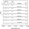 |
Fig. 1 Spectra of our five sample stars, ranked by decreasing value of [Fe/H], in the region of MgI. For comparison two Milky Way halo stars are included, HD 122563 and CD −38 245, at [Fe/H] = −2.8 and [Fe/H] = −4.19, respectively. |
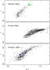 |
Fig. 2 Reddening corrected color − magnitude diagrams of Sextans, Fornax, and Sculptor for our galaxy members selected from their spectra in the CaT region. |
3. Stellar parameters
3.1. Stellar models
Photospheric 1D models for the sample giants were extracted from the new MARCS2 spherical model atmosphere grids (Gustafsson et al. 2003, 2008). The abundance analysis and the spectral synthesis calculations were performed with the code calrai, first developed by Spite (1967) (see also the atomic part description in Cayrel et al. 1991), and continuously updated over the years. This code assumes local thermodynamic equilibrium (LTE), and performs the radiative transfer in a a plane-parallel geometry.
The program calrai is used to analyze all DART datasets and in particular the VLT/giraffe spectroscopy of Fornax, Sculptor, and Sextans dSphs (Hill et al. in prep.; Letarte et al., 2010; Tafelmeyer et al., in prep.). The results of these works are partly summarized in Tolstoy et al. (2009). The homogeneity of the analyses allows secure comparisons of the chemical patterns in all metallicity ranges and between galaxies.
As we discuss in a following subsection, we had to combine the results provided by calrai with those of turbospectrum (Alvarez & Plez 1998) in order to properly take into account the continuum scattering in the stellar atmosphere for the abundances derived from lines in the blue part of the spectra. We have conducted a series of tests on HD 122563 and CD−38 245, sampling the two extremes of our metallicity range, to verify the compatibility of the two codes. In all these tests, the continuum scattering is treated as absorption in order to put both codes on same ground. Both calrai and the version of turbospectrum adopted for our calculations use spherical model atmospheres and plane-parallel transfer for the line formation, also referred to sp computations in the terminology of Heiter & Eriksson (2006). These authors recommend the use of spherical model atmospheres in abundance analyses for stars with log g ≤ 2 and 4000 ≤ Teff ≤ 6500 K, and our target stars fall into this range. As they point out, geometry has a small effect on line formation and a plane-parallel transfer in a spherical model atmosphere gives excellent results with systematics below 0.1 dex compared to a fully spherical treatment.
Visual and near-IR photometry.
Because the original abundances of HD 122563 and CD−38 245 were derived by Cayrel et al. (2004) using MARCS plane-parallel models (pp computations) and an earlier version of turbospectrum, we proceeded to reproduce their results with our techniques. We first checked that we could reproduce the abundances of Cayrel et al. (2004) with pp computation of the current version of turbospectrum: they agree within 1/1000 th of a dex. Moving from pp turbospectrum computations to sp induces a mean −0.056 ± 0.04 dex shift for CD−38 245 and −0.12 ± 0.07 dex for HD 122563 for all iron lines (iron is taken here as reference, as it provides the largest number of lines). Considering only lines with excitation potential above 1.4 eV, as we do in the analysis of our dSph star sample, the mean difference in iron abundance between the sp versions of turbospectrum and calrai is −0.003 and −0.08 dex for CD−38 245 and HD 122563, respectively. Restricting our analysis to FeI and to lines with excitation potential larger than 1.4 eV, we get a difference of −0.038 ± 0.04 dex and −0.108 ± 0.04 for CD−38 245 and HD 122563, respectively. These numbers perfectly agree with the work of Heiter & Eriksson (2006), which describes the difference between sp and fully spherical ss models increasing with decreasing stellar gravity and increasing effective temperature. The variation in stellar gravity is the primary factor of systematics between spherical and parallel models. CD−38 245 is hotter than HD 122563 by only 200 K, but its gravity is 0.4 dex larger.
If we consider all chemical elements and lines for our sample stars and keep the same atmospheric parameters, the mean of the difference in abundances between the programs calrai and turbospectrum for lines with an excitation potential larger than 1.4 eV are 0.03 (std = 0.05) for Fn05-42, −0.02 (std = 0.05) for Scl07-49, −0.01 (std = 0.03) for Scl07-50, 0.02 (std = 0.08) for Sex11-04, and −0.05 (std = 0.06) for Sex24-72. These values are reached when both codes consider scattering as absorption.
In conclusion, calrai and turbospectrum lead to highly compatible results, well within our observational error bars, and their results can be combined with confidence.
3.2. Photometric parameters
Optical photometry (V, I) was available for our sample stars from the ESO 2.2 m WFI (Tolstoy et al. 2004; Battaglia et al. 2006, 2010). This was supplemented by near-infrared J, H, Ks photometry from 2MASS (Skrutskie et al. 2006) and from J, K photometry made available from VISTA commissioning data, which were also calibrated onto the 2MASS photometric system. Table 2 presents the corresponding stellar magnitudes.
With the exception of the Sculptor stars, for which we have no H-band data, we considered four different colors V − I, V − J, V − H and V − Ks and the CaT metallicity estimates to get initial values of Teff, following the calibration of Ramírez & Meléndez (2005), with a reddening law (A(V) / E(B − V) = 3.24) and extinction of E(B − V) = 0.05, 0.017 and 0.02 for Sextans, Sculptor, and Fornax, respectively (Schlegel et al. 1998). The calibration of Ramírez & Meléndez (2005) is our temperature calibration for all DART samples. It has the advantage of using the same photometric system as our observations, avoiding precarious Johnson-Cousin system conversions and thereby providing a more robust Teff scale.
The photometric surface gravities were calculated using the standard relation
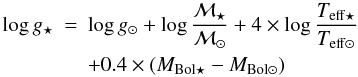 with
log g⊙ = 4.44, Teff ⊙ = 5790 K
and MBol ⋆ the absolute bolometric magnitude
calculated from the V-band magnitude using the calibration for the
bolometric correction from Alonso et al. (1999),
assuming distances of 140 kpc for Fornax and 90 kpc for Sextans and Sculptor (Karachentsev et al. 2004). The mass of the RGB stars
was assumed to be ℳ ⋆ = 0.8 ℳ⊙.
with
log g⊙ = 4.44, Teff ⊙ = 5790 K
and MBol ⋆ the absolute bolometric magnitude
calculated from the V-band magnitude using the calibration for the
bolometric correction from Alonso et al. (1999),
assuming distances of 140 kpc for Fornax and 90 kpc for Sextans and Sculptor (Karachentsev et al. 2004). The mass of the RGB stars
was assumed to be ℳ ⋆ = 0.8 ℳ⊙.
3.3. Spectroscopic metallicities, temperatures, and microturbulence velocities
The effective temperatures and microturbulence velocities (vmic) were determined spectroscopically from lines of FeI by requiring no trend of abundance with either excitation potential or equivalent width. According to Magain (1984), random errors on equivalent widths can cause a systematic bias in the derived microturbulence velocities. This effect is caused by the correlation of the error on each equivalent width and the abundance deduced from it, and can be avoided by using predicted equivalent widths instead of measured ones in the plot of iron abundances vs. equivalent widths. The former are calculated using the line’s log gf value and excitation potential and the stellar atmospheric parameters. They are thus free of random errors and yield unbiased microturbulence velocities. We estimated the change in velocities that would compensate for the differences of slopes when changing to predicted equivalent widths, and found that much less than 0.1 km s-1 was sufficient in all cases. This is small compared to the uncertainties given in Sect. 3.4. We nevertheless used the predicted equivalent widths instead of the measured ones for the Sextans stars with [Fe/H] ≥ −3. Extrapolation of the model atmospheres, which was necessary for the metallicity domain below −3, can cause errors in the predicted equivalent widths, therefore they were not used for the remaining more metal poor stars of our sample.
Photometric and spectroscopic stellar parameters.
Surface gravities are often determined spectroscopically by requiring iron to have ionization equilibrium. For our sample stars, [FeI/H] abundances were determined from 20 − 70 FeI lines per star, depending on S / N and metallicity. However, the FeII abundances were deduced from a small number (2 to 4) of weak lines and were consequently fairly uncertain. Moreover, the atmospheres of metal-poor stars are characterized by low electron number densities and low opacities. Hence local thermodynamical equilibrium (LTE) is not fulfilled in the atmospheric layers where these lines are formed. The main non-LTE effect on iron is over-ionization, which is caused by photo-ionization of excited FeI lines from a super-thermal radiation field in the UV (see e.g. Asplund 2005,and references therein). Therefore we did not use spectroscopic gravities but rather kept the photometric ones. Note that all our stars, except Scl07-50, have higher iron abundances when derived from ionized species instead of neutral ones. Even though the differences are typically within the errors, we see this as clear evidence for over-ionization owing to NLTE effects. The situation is even clearer for titanium, with differences between [TiI/H] and [TiII/H] of ~0.4 dex. The first ionization potential of titanium is slightly lower than that of iron, while the second ionization potential is roughly the same. Therefore one expects the overionization caused by the UV radiation field to be more prominent for titanium than for iron. Moreover, almost all Ti i lines measured here arise from low excitation levels, and are therefore also more prone to NLTE effects on the level population than the higher excitation Fe i lines.
For Scl07-049, we count ≈20 FeI lines (≈50% of the total number of FeI lines) with excitation potentials below 1.4 eV. They may well be affected by non-LTE effects, as these are particularly important for low excitation lines. This influences the atmospheric parameters by biasing the diagnostic slopes and the metallicities. Hence, these lines were not considered, neither for the determination of the mean metallicity nor for the effective temperature. For Fnx05-042 the influence of these lines was negligible, thus they were kept in the analysis. The fraction of low excitation lines is much smaller in the case of the two Sextans stars and Scl07-050 (10 to 20% of the total). Hence, all lines were included.
3.4. Final atmospheric parameters and error estimates
The convergence to our final atmospheric parameters, presented in Table 3, was achieved iteratively, as a trade-off between minimizing the trends of metallicity with excitation potentials and equivalent widths on the one hand and minimizing the difference between photometric and spectroscopic temperatures on the other hand. We started from the photometric parameters and adjusted Teff and vt by minimizing the slopes of the diagnostic plots, allowing for deviation by no more than 2σ of the slopes. This yielded new metallicities, which were then again fed into the photometric calibration to derive new photometric temperatures and gravities. In this way, after no more than two or three iterations, we converged on our final atmospheric parameters. The errors in atmospheric parameters, +150 K for Teff +0.2 km s-1 for vt and +0.3 dex log (g), also reported in Table 4, reflect the range of parameters over which we can fulfill our conditions of both minimal slopes in the diagnostic plots and small difference between photometric and spectroscopic temperatures.
However, there is a strong correlation between excitation potential and equivalent width, in the sense that the majority of the weak lines have high excitation potentials, and most of the strong lines have low excitation potentials. Therefore, Teff and vt cannot be determined independently from each other. To a certain degree, it is possible to compensate for an uncertainty in one parameter by modifying the other. ΔTeff = 150 K is the maximum variation in effective temperature that could still lead to an acceptable solution, and Δvt = 0.2 km s-1 is the corresponding change in microturbulence velocity keeping the slopes between abundance and equivalent width or excitation potential to zero within 2σ.
Errors owing to uncertainties in stellar atmospheric parameters.
4. Determination of abundances
Our line list (shown in Table 6) combines the compilation of Shetrone et al. (2003), François et al. (2007) and Cayrel et al. (2004). The solar abundances of Anders & Grevesse (1989) are adopted, with the exception of C, Ti, and Fe (Grevesse & Sauval 1998). In the following all abundances, including those of the comparison samples, are scaled to these solar values. All abundances are listed in Table 7 and they were derived from the equivalent widths, with the exception of those marked in Table 6.
4.1. The influence of scattering
The color − magnitude diagrams in Fig. 2 show that the stars from our sample are located close to the tip of the RGB. Thus, at low metallicity and low temperature, a proper treatment of continuum scattering in the stellar atmosphere is mandatory.
Our standard line formation code, calrai, treats continuum scattering as if it were absorption in the source function, i.e., Sν = Bν, an approximation that is valid at long wavelengths. In the blue, however, the scattering term must be explicitly taken into account: Sν = (κν × Bν + σν × Jν) / (κν + σν). Cayrel et al. (2004) have shown that the ratio σ/κ in the continuum is 5.2 at λ = 350 nm, whereas it is only 0.08 at λ = 500 nm, for τν = 1 and a giant star with Teff = 4600 K, log g = 1.0, and [Fe/H] = −3. Therefore, we used the code turbospectrum (Alvarez & Plez 1998), which includes the proper treatment of scattering in the source function, to correct our original calrai abundances.
Figure 3 illustrates how scattering influences the abundances. All calculations are done with turbospectrum. In the lower panel, we plot the differences in abundances between those derived assuming a pure absorption source function and those explicitly including a scattering term. Abundances tend to be overestimated when scattering is not properly taken into account, and the main driver of the scattering effect is the line wavelength. In addition, the lower the gravity, the larger the effect of continuum scattering. There is also mild evidence that the higher the excitation potential of the lines, the larger the differences between the abundance estimates. This is a consequence of the increase in formation depth of the lines. In conclusion, the corrections for some of our stars can be large because of the combined effects of being very metal poor and high up on the RGB (luminous and cool). The upper panel in Fig. 3 shows, with the example of [FeI/H], that when scattering is properly treated, no spurious wavelength dependence remains. The larger dispersion at bluer wavelengths arises from lower signal-to-noise ratio spectra in this domain.
To avoid any bias in the effective temperatures, we did not consider the iron lines at short wavelengths, because they have large scattering corrections, but instead restricted our analyses to iron lines at λ > 4800 Å. The only exception to this rule is Scl07-050, for which we could detect only around 10 lines with λ > 4800 Å. Therefore we used the blue lines as well for the sake of better statistics. However, as Fig. 3 shows, Scl07-050 has the smallest influence of scattering, never exceeding 0.2 dex, even at the lowest wavelengths. We estimated that the bias in the slopes of iron abundances vs. excitation potentials causes errors in effective temperatures of no more than 30 K. This is negligible compared to the uncertainties given in Table 4.
In summary, our method has been the following: calrai was used to determine the stellar atmospheric parameters. These parameters were kept unchanged. The abundances were corrected line-by-line using turbospectrum in two modes: (i) treating continuum scattering as if it were absorption in the source function; (ii) with a proper scattering term in the source function. The difference between the two outputs was then applied to the calrai abundances. The corrections are listed in Table 6.
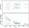 |
Fig. 3 Lower panel: the differences in abundances derived assuming a pure absorption source function and when a scattering term is introduced. All calculations are done with turbospectrum. All lines are considered and are shown at their wavelengths. Black points trace Fnx05-42, blue stands for the 2 Sextans stars, red for Scl07-49 and green for Scl07-50. Upper panel: [FeI/H] when scattering is properly taken into account. There is no trend of abundance with wavelength, while there was a clear increase at bluer wavelengths before correction. |
4.2. Errors
The errors given in Table 7 and shown in the
figures were derived in the following way: Although we used splot to measure the line
equivalent widths, we used the error estimates of DAOSPEC, which provide the uncertainty
in equivalent width, ΔEW, derived from the residual of the Gaussian fit.
This includes the uncertainties in the placement of the continuum. We propagated this
ΔEW throughout the abundance determination process, thus providing for
each line δDAO, the abundance uncertainty corresponding to
EW ± ΔEW. The abundance uncertainty is not necessarily
symmetric, and in all cases we adopted the largest one. For the lines for which abundances
were determined from synthetic spectra, δDAO was estimated
from the range of abundances for which a good fit of the observed line profile could be
achieved. For the abundance of elements measured from more than one line, the mean
abundance and dispersion (σ(X)) were computed, weighting the lines by
1/ . The corresponding error on the mean,
δσ, is given as
. The corresponding error on the mean,
δσ, is given as  , where NX is the number of
lines used to determine the abundance of element X. In order to avoid artificially small
errors due to low number statistics when too few lines were available to measure a robust
σ(X), we took as a minimum for σ(X), the dispersion of
Fe abundances and assumed
, where NX is the number of
lines used to determine the abundance of element X. In order to avoid artificially small
errors due to low number statistics when too few lines were available to measure a robust
σ(X), we took as a minimum for σ(X), the dispersion of
Fe abundances and assumed  as the smallest possible error value. The final error in
[X/H] is then max(δDAO,
δσ, δFe). To
get the error in [X/Fe], the uncertainty of [Fe/H] was added in quadrature.
as the smallest possible error value. The final error in
[X/H] is then max(δDAO,
δσ, δFe). To
get the error in [X/Fe], the uncertainty of [Fe/H] was added in quadrature.
The considerations above do not contain errors due to uncertainties in the atmospheric parameters. As explained in Sect. 3, there is a strong correlation between micro-turbulence velocity and effective temperature. Therefore we give errors as a combination of ΔT and Δvmic. The error boundaries reflect the parameter range for which the slopes of both diagnostic plots (excitation potential and equivalent widths versus iron abundance) can be brought close to zero.
4.3. Abundances not based on equivalent widths
Some of the lines, primarily in the blue, gave uncertainties of 0.5 dex or more. The reasons for this are manifold: extremely strong lines (~300 mÅ), large residuals of the Gaussian fit because of low S / N, problems of continuum placement (caused by low S / N or broad absorption bands in the vicinity), very strong blends. Whenever possible, we did not use these lines and used instead those in the red part of the spectrum. For the elements for which this strategy could not be adopted, the abundances were determined from synthetic spectra:
-
(i)
Hyperfine structure: the abundances of barium, cobalt,manganese, and scandium from the red lines were determinedfrom spectral synthesis, in order to consider hyperfine splitting ofthe lines. The atomic data of the hyperfine components were takenfrom Prochaska et al. (2000) and, ifno data were given there, from Kuruczdatabase3. For the threeblue lines of scandium at 4246.82 Å,4314.08 Å, and4400.39 Å no hfsdata were available, hence we did not correct the abundances.
-
(ii)
Blends: if there were significant blends, the abundances were derived from synthesis to correct for the contribution of these blends. The silicon and aluminum lines of Sex24-72 were blended by molecular bands, the Al line at 3944.01 Å and the Si line at 3905.52 Å were not used at all, since the blends were too strong. The chromium abundance of the line at 5208.42 Å was larger than the abundances derived from the other lines by 0.3−0.5 dex in all stars. The synthetic spectra revealed the presence of an iron blend. After taking this into consideration, the abundance of the 5208.42 Å line agreed well with the other chromium lines. The abundances of two magnesium lines, which lie close to a strong hydrogen line at 3835.38 Å, were determined with synthesis, to make sure that their abundances were not affected by the H line wings.
-
(iii)
Very weak or strong lines: the equivalent widths were determined from Gaussian fits to the line profile. However, for strong lines (≳ 250 mÅ), this might not give correct results due to the presence of significant wings. Similarly, if lines are too weak and narrow (≲ 20 mÅ), the line profile may deviate from a Gaussian shape and therefore a Gaussian fit can be incorrect. Thus, for elements for which only very weak or very strong lines were available, abundances were determined from spectral synthesis: the two sodium resonance lines of Sex24-72 at 5889.97 Å and 5895.92 Å (the uncertainty in [Na/H] derived from the line at 5889.97 Å was much larger than 0.5 dex, therefore only the other line is used here) and the very weak yttrium line in Sex11-04.
5. Results
5.1. Comparison samples
We compare our results with high-resolution spectroscopic analyses of RGBs with [Fe/H] ≤ −2.5 in the Milky Way halo (Cayrel et al. 2004; Cohen et al. 2008; Aoki et al. 2005, 2007; Cohen et al. 2006; Lai et al. 2008; Honda et al. 2004) and in faint (Ursa MajorII and Coma Berenices, Boötes I, Leo IV) and classical (Sextans, Draco, Fornax, Carina, Sculptor) dSphs (Letarte et al. 2010; Shetrone et al. 2001; Fulbright et al. 2004; Koch et al. 2008a; Cohen & Huang 2009; Aoki et al. 2009; Norris et al. 2010; Simon et al. 2010; Frebel et al. 2010b,a). We distinguish between unmixed and mixed RGBs in order to be able to draw a reliable comparison sample for the elements that are sensitive to mixing. The term “mixed” refers to stars for which the material from deep layers, where carbon is converted into nitrogen, has been brought to the surface during previous mixing episodes. Mixing has occurred between the atmosphere of RGB stars and the H-burning layer where C is converted into N by the CNO cycle (Cayrel et al. 2004).
Following Spite et al. (2005) and Spite et al. (2006), we divide stars into these two
categories according to their carbon and nitrogen abundances or the ratio between the
carbon isotopes 12C and 13C, when possible. The criteria are
[C/N] ≤ −0.6 or log (12C/13C) ≤ 1 for mixed stars and
[C/N] > −0.6 or log (12C/13C) > 1 for unmixed ones.
Figure 4 presents the log g vs.
Teff diagram for our comparison sample and the stars
analyzed in this paper. Mixed stars are generally more evolved and are located on the
upper RGB above the RGB bump luminosity (Gratton et al.
2000). The luminosity of the RGB bump decreases with increasing metallicity
(Fusi Pecci et al. 1990). At [Fe/H] < −2.5 it
is predicted around  (Spite et al. 2006,
Lagarde & Charbonnel, priv. comm.). None of our dSph stars have N
abundances, therefore, we rely on their location at the top of the log g
vs. Teff diagram to conclude that they are indeed mixed stars.
(Spite et al. 2006,
Lagarde & Charbonnel, priv. comm.). None of our dSph stars have N
abundances, therefore, we rely on their location at the top of the log g
vs. Teff diagram to conclude that they are indeed mixed stars.
The abundances of our comparison sample have been derived using plane-parallel atmospheric models. We have run calrai with plane-parallel atmospheric models (Gustafsson et al. 1975) on our sample stars. The effective temperatures were changed by less than 100 K. There was no systematic shift in abundances. The mean differences in abundances ([M/H]) derived in pp and sp models are well within the observational errors: 0.04 dex (std = 0.04) for Sex24-72, 0.02 dex (std = 0.09) for Sex11-04, 0.005 dex (std = 0.13) for Fnx05-42, −0.038 (std = 0.05) for Scl07-49, and 0.005 (std = 0.017) for Scl07-50. Similarly, the abundance ratios were modified by 0.005 dex (std = 0.04) for Sex24-72, −0.05 dex (std = 0.09) for Sex11-04, −0.03 dex (std = 0.13) for Fnx05-42, −0.002 (std = 0.05) for Scl07-49, and −0.003 (std = 0.018) for Scl07-50. As a conclusion, samples can be safely inter-compared.
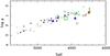 |
Fig. 4 DART dSph targets are in color: Sextans(Green) Scl(Blue) Fnx (Red). Large triangles identify the 5 stars analyzed here, while small triangles indicate stars in earlier publications (Letarte et al. 2010; Aoki et al. 2009; Shetrone et al. 2001; Frebel et al. 2010a). Open squares: UFDs, Carina and Draco (Fulbright et al. 2004; Koch et al. 2008a,b; Frebel et al. 2010b; Cohen & Huang 2009; Norris et al. 2010; Simon et al. 2010). The Milky Way halo stars are represented by circles; open circles are unmixed RGBs and filled circles mixed RGBs (Cayrel et al. 2004; Cohen et al. 2008; Aoki et al. 2005; Spite et al. 2005; Aoki et al. 2007; Cohen et al. 2006; Lai et al. 2008; Honda et al. 2004). |
5.2. Iron
Our results place all our sample stars at [Fe/H] ≲ −3 and three stars below [Fe/H] ~ −3.5. This constitutes the first clear evidence that likely all classical dSphs contain extremely metal-poor stars.
While the detailed abundances of our sample stars are presented here after full analysis, the existence of Scl07-50 and other EMPS in classical dSphs was already reported earlier (Hill 2010; Tolstoy 2010). Scl07-50 at [Fe/H] = −3.96 ± 0.06 is the most metal-poor star ever observed in an external galaxy, but more fundamentally, it considerably revises the metallicity floor of dSphs, setting it at comparable level with the Milky-Way. Figure 5 compares the equivalent widths of CD−38 245 and Scl07-50, which have very similar atmospheric parameters. The lines of CD−38 245 are on average ~20 mÅ weaker, corresponding to the ~0.2 dex difference in metallicity between the two stars.
In Fig. 6 our UVES high-resolution [Fe/H] values are compared to the FLAMES LR [Fe/H] estimates derived from the CaT (with the calibration of Battaglia et al. 2008) for Sex11-04, Fnx05-42, Scl07-49 and Scl07-50 and from R ~ 18000 spectroscopy at the HET for Sex24-72.
It is obvious that for [Fe/H] ≲ −2.5, the traditional method based on the CaT absorption features predicts a metallicity that is too high. The underlying physical reasons for this has recently been explained by Starkenburg et al. (2010), who show that it reflects the change of the profile of the CaT lines, from wing-dominated to core dominated as the metallicity drops. They provide a new calibration which is valid down to [Fe/H] = −4. Figure 6 indicate with arrows the corresponding new CaT metallicities for stars of the present sample.
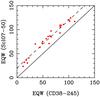 |
Fig. 5 The comparison of the equivalent widths of Scl05-50 ([Fe/H] = −3.96) and the Milky Way halo star CD−38 245 ([Fe/H] = −4.19). The dashed lined follows the mean ~20 mÅ difference between the equivalent widths of the two stars. |
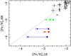 |
Fig. 6 Comparison for our sample stars between [Fe/H] from high resolution UVES measurements ([Fe/H]HR) and that from the CaT with the calibration of Battaglia et al. (2008) ([Fe/H]LR), as filled circles. For Sex24-72 HET/HRS spectroscopy at R ~ 18000 is used because CaT data are not available. Blue stands for the Sculptor’s stars, red for the Fornax’ star, and green is for Sextans’s ones. The CaT metallicity determined with the new calibration of Starkenburg et al. (2010) for low metallicities are shown as open circles. Crosses provide the same comparison at [Fe/H] > −2.5, where the classical (old) CaT calibration is robust. |
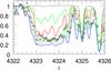 |
Fig. 7 Synthesis of the molecular CH band at 4323 Å of Sex24-72. The crosses are the observed spectrum, the red line corresponds to the synthetic spectrum with [C/Fe] = 0.0, the green lines are for [C/Fe] = ± 0.5, the blue line is for [C/Fe] = 1.0, and the black line for the complete absence of C. |
5.3. Carbon
Carbon abundances were determined from synthesis of the CH molecular bands in the blue part of the spectrum. As an example, Fig. 7 shows the synthesis of the CH band at 4323 Å for Sex24-72. Because calrai does not include molecular bands, the synthetic spectra were calculated with turbospectrum using the same CH line list as in Cayrel et al. (2004). The carbon abundances are sensitive to the assumed oxygen abundances through the locking of C into the CO molecule. We only have upper limits for oxygen, hence we used Mg as an indicator of the oxygen abundance, assuming [O/H] = [Mg/H]. Increasing by +0.2 dex the adopted [O/Fe] translates into a maximum increase of +0.05 of the derived C abundance (the exact dependence is a function of the absolute C/O ratio in the star). This uncertainty is negligible with respect to the errors on the fits to the data in combination with a poor signal-to-noise ratio and uncertainties associated with the molecular lines’ oscillator strengths.
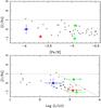 |
Fig. 8 DART dSph targets are in colored triangles: Sextans(Green) Scl(Blue) Fnx (Red). Other symbols are squares (Ursa MajorII), triangles (Coma Berenices), diamonds (Draco), star (Boötes) (Fulbright et al. 2004; Koch et al. 2008a; Frebel et al. 2010b; Cohen & Huang 2009; Norris et al. 2010). Only mixed Milky Way halo stars (black dots) are considered (Cayrel et al. 2004; Cohen et al. 2008; Honda et al. 2004; Aoki et al. 2005, 2007; Cohen et al. 2006; Lai et al. 2008). The dashed line delineates the regions in which they are observed. |
Figure 8 shows [C/Fe] as a function of the stellar
metallicity and luminosity for our sample stars, drawing a comparison with the Milky Way
halo, Draco, Boötes I, Ursa Major II and Coma Berenices EMPS. The [C/Fe] does not depend
on metallicity. The bolometric luminosities are derived from the gravities and effective
temperatures, assuming a mass of ℳ = 0.8 ℳ⊙ for all stars. The first clear
result is that none of our stars is C-rich in the classical sense ([C/Fe] > 1). All
but one star, Sex24-72, have [C/Fe] ≤ 0 as expected for their tip-RGB luminosities (Spite et al. 2005). The onset of the extra mixing
(δμ) lies at  for a 0.8 star. Eggleton
et al. (2008) also show a metallicity dependence of the luminosity at the onset
of the mixing, increasing from
for a 0.8 star. Eggleton
et al. (2008) also show a metallicity dependence of the luminosity at the onset
of the mixing, increasing from  to 2.4 for metallicity passing from 0.02 (solar) to 0.0001
(−2.3). An independent evidence confirming that our sample stars have experienced
thermohaline convection comes from the low ratio
12C/13C = 6
to 2.4 for metallicity passing from 0.02 (solar) to 0.0001
(−2.3). An independent evidence confirming that our sample stars have experienced
thermohaline convection comes from the low ratio
12C/13C = 6 , that we measure in Sex24-72, the most C-rich star of our
sample, in which this can be done (Spite et al.
2006).
, that we measure in Sex24-72, the most C-rich star of our
sample, in which this can be done (Spite et al.
2006).
Aoki et al. (2007) argued that given that mixing on
the RGB and extra mixing at the tip of the RGB lower the surface abundance of carbon in
late-type stars compared to their earlier stage of evolution, the definition of
carbon-enriched EMP stars (CEMPS) should depend on the stellar luminosity. Hence, for
 , a giant star would be considered CEMPS for [C/Fe] > 0.
Applying this criterion, one Sextans star of our sample, Sex24-72 with
[C/Fe] = 0.4 ± 0.19, is carbon enhanced.
, a giant star would be considered CEMPS for [C/Fe] > 0.
Applying this criterion, one Sextans star of our sample, Sex24-72 with
[C/Fe] = 0.4 ± 0.19, is carbon enhanced.
Both Frebel et al. (2010b) and Cohen & Huang (2009) reported similar cases in Ursa Major II and in Draco. We note that Frebel et al. (2010b) measure [C/Fe] = −0.07 ± 0.15 for HD 122563, which they use as reference, while Spite et al. (2005) calculated [C/Fe] = −0.47 ± 0.11 for the same star. Part of this apparent discrepancy results from differences in the C and Fe solar abundances, which induces a 0.08 dex shift. Frebel et al. [C/Fe] = −0.15 ± 0.15 in Spite et al.’s scale. The effective temperature difference between the two studies (100 K) cannot explain the difference. Indeed, increasing Frebel et al. (2010b)’s Teff by this amount would actually increase [C/Fe] by + 0.07 dex and lead to an even larger discrepancy. Taking the same atmospheric parameters as Spite et al. (2005) for HD 122563, but using spherical models as we do for the dSph stars, we derived [C/Fe] = −0.6 ± 0.13. Taking into account the 0.03 dex difference in the C and Fe solar abundances between the two works, our abundance ratio is −0.57 ± 0.13 in Spite et al. scale, i.e., fully compatible. Moreover, we checked that this 0.1 dex difference was entirely caused by passing from pp to sp models.
An immediate consequence of the checking result on HD 122563 is that Sex24-72 is definitely carbon-rich (since we seem to tend to have low carbon abundances). Another consequence is to attribute a maximum uncertainty of ~0.3 dex in the carbon abundances of Frebel et al. (2010). Shifting all of their [C/Fe] values downward by this amount does not change their identification of a C-rich star in Ursa Major II.
The origin and nature of these moderately enhanced carbon stars in dSphs and ultra faint dwarfs (UFDs) is intriguing, because they are not observed in our Galaxy. Mass transfer by a companion AGB is an unlikely hypothesis: we would expect a higher [C/Fe] than is observed at these very low metallicities, because low metallicity AGBs tend to produce more carbon than metal-rich ones (Cristallo et al. 2009; Bisterzo et al. 2010; Suda & Fujimoto 2010; Karakas 2010), and because the efficiency of carbon-depletion is significantly reduced in these carbon-rich stars (Denissenkov & Pinsonneault 2008; Stancliffe et al. 2009). This is often accompanied by an increase in magnesium abundance, while Sex24-72 [Mg/Fe] is not high. All this suggests a pristine carbon enrichment. Another piece of evidence is the very low [Ba/H] of the stars with [C/Fe] > 0. A vast majority of Milky Way carbon-rich stars are also over-abundant in barium, hence one would expect that the C-rich stars would also be Ba-rich (e.g. Beers & Christlieb 2005; Aoki et al. 2007).
Our two stars in Sextans are located very close to each other in the HR diagram, share the same metallicity, and for most of the other elements have the same abundance ratios. C appears to be a significant exception and probably requires primordial C inhomogeneities. We note that this dispersion in [C/Fe] has so far only been seen in low-luminosity dSphs. Simulations of Revaz et al. (2009) suggest that these small systems are prone to significant dispersion in elemental abundances, as a consequence of their sensitivity to feedback/cooling processes during their star formation histories. Meynet et al. (2006) show that rotating massive stars can loose a large amount of carbon enhanced material. When these ejecta are diluted with supernovae ejecta, the [C/Fe] abundance ratios are very similar to those observed in CEMPs. This mechanism for the very early production of significant amounts of carbon together with classical abundances for the other elements, should be more easy to detect in low-mass dSphs than in higher mass systems, owing to poor mixing in the early phases of star formation. Clearly larger samples of stars are needed to cover the entire mass range of the dSph galaxies and properly test this hypothesis.
We note that the dispersion in [C/Fe] (1.4 dex) among Sextans stars with similar luminosities echoes the spread in abundances of other elements for this galaxy. This does not imply that this dispersion is the rule in other dSphs, in particular when they experience very different star formation histories. We note however that star-to-star variation in carbon is also seen in Draco. This is in contrast to the homogeneity seen in other elements, implying a specific process leading to the spread in carbon.
5.4. Oxygen
None of the forbidden lines at 6300 Å and 6363 Å could be detected, hence only upper limits could be derived. For the two Sculptor stars these limits were clearly above [O/Fe] ≳ +2.0 and consequently disregarded. The upper limits for the other stars can be found in Table 7.
5.5. The even-Z elements
5.5.1. Abundances
The Mg abundances were generally determined from the lines in the red part of the spectrum, at 5172 Å, 5183 Å, and 5528 Å. In the case of Scl07-050, two blue lines at 3829 Å and 3832 Å were available as well. These lines are in the region that is affected by continuum scattering and close to the strong H 3835 Å line, whose wings influence the continuum. Therefore we did spectral synthesis for these two blue lines.
For Si, two blue lines at 3905.5 Å and 4102.9 Å could be used in principle for all stars. However, for the most C-rich star in our sample, Sex24-72, synthesis showed that both lines are blended by molecular bands. The 3905.5 Å even vanishes completely within a strong molecular line and can therefore not be used. Hence, for the two Sextans stars and Fnx05-42, we only used the 4102.9 Å line. For Scl07-050, only the line at 3905 Å is used, since the other one is too weak to be detected. We miss the blue part of Scl07-049 spectrum, therefore we could only get an upper limit for from the extremely weak red line at 5684.52 Å.
The Ca abundance is generally derived from the six lines at 5589 Å, 5857 Å, 6103 Å, 5122 Å, 6162 Å, and 6439 Å, or from a subset of these six lines for the stars with lower Ca abundances. However, for Scl07-050, none of these six lines was detectable. Therefore its Ca abundance is based on only one blue line at 4227 Å. This line is not considered for the other stars, since it is in the very low S / N region. This line is a resonance line and very sensitive to NLTE effect as reflected by the suspiciously low [Ca/Fe] of Scl07-050, which does not reflect the abundance ratios of the other α-elements for this star.
The TiI abundances were determined from three to seven lines in the red part of the spectra for all stars with the exception of Scl07-050, for which no TiI line could be detected at all. For this star an upper limit for [TiI/Fe] of +0.35 dex is derived from the line at 4981 Å. Generally all TiI lines are very weak, with a large fraction of lines having equivalent widths between 20 mÅ and 40 mÅ. The TiII abundances were mainly derived from three to seven red lines. Most of the blue lines had to be disregarded because of too low S / N. The few blue lines that were not removed gave abundances very close to the ones determined from the red lines. Again, Scl07-50 is an exception, since no red line of TiII could be detected. Hence, its TiII abundance is based on its nine blue lines.
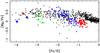 |
Fig. 9 DART dSph targets are in colored triangles: Sextans(Green) Scl(Blue) Fnx (Red). Large symbols stand for the sample stars of this work, small ones stand for earlier works and publications (Hill et al., in prep.; Letarte et al. 2010; Frebel et al. 2010a; Aoki et al. 2009; Shetrone et al. 2001). Other symbols are squares (Ursa MajorII, Frebel et al. 2010b), triangles (Coma Berenices, Frebel et al. 2010b), diamonds (Draco, Shetrone et al. 2001; Fulbright et al. 2004; Cohen & Huang 2009), star (Boötes, Norris et al. 2010), cross (Carina, Shetrone et al. 2003; Koch et al. 2008a), and circle (Leo IV, Simon et al. 2010). All Milky Way halo stars from our comparison sample are considered (black dots) Cayrel et al. (2004); Honda et al. (2004); Aoki et al. (2005, 2007); Cohen et al. (2006, 2008); Lai et al. (2008). For the purpose of this figure, Venn et al. (2004)’s compilation was added at [Fe/H] ≥ −2.5. |
5.5.2. Analysis
Figure 9 presents [Mg/Fe] as a function of [Fe/H] for all dSph galaxies for which very metal poor and/or extremely metal poor stars have been found and abundances measured based on high-resolution spectroscopy. It extends the metallicity range covered up to [Fe/H]=0 in order to include the full chemical evolution of the dSph galaxies and make a clear comparison with the Milky Way. Our choice of magnesium was driven because it is the most extensively measured α-element. We included the abundance ratios derived by Shetrone et al. (2003) in Carina at [Fe/H] ≳ −2 and those compiled by Venn et al. (2004) in the Galactic halo for [Fe/H] ≳ −2.5.
From the faintest UFDs to the most luminous of the classical dSphs and to the Milky Way, Fig. 9 samples nearly the full range of dwarf galaxy masses, allowing common as well as distinct features to be uncovered. Below [Fe/H] ~ −3, galaxies are essentially indistinguishable. This means that the very first stages of star formation in galaxies have universal properties, both in terms of nucleosynthesis in massive stars and physical conditions triggering star formation. This was also foreseen by Frebel et al. (2010b,a); Simon et al. (2010). Conversely, at [Fe/H] ≳ −2 galaxies have clearly imprinted the peculiarities of their star formation histories in their abundance ratios: the explosions of type Ia supernovae (SNe Ia) occur at lower global enrichment in iron for lower star formation efficiency (see also Tolstoy et al. 2009). In between these two extremes, at least one galaxy, Sextans, shows signs of inhomogeneous interstellar medium, revealed by the dispersion in [Mg/Fe] for stars of similar [Fe/H]. Although solar [Mg/Fe] are observed in Milky Way halo very metal-poor stars, their fraction over the total number of observed stars is significantly larger in Sextans. Aoki et al. (2009) attributes the origin of low [Mg/Fe] as likely due to low-mass type II supernovae, but Revaz et al. (2009) show that even as low as [Fe/H] ~ −2.7, SNe Ia would have time to explode. Only larger samples will be able to solve this matter.
While magnesium is produced in hydrostatic nuclear burning phase in type II SN progenitors, the synthesis of silicon to calcium comes partly from the presupernova explosion but is also augmented by an important contribution from explosive oxygen burning in the shock (Woosley & Weaver 1986). [Si/Fe], [Ti/Fe], [Ca/Fe] are shown in Fig. 10 and hardly display any differences from [Mg/Fe] in the same metallicity range, once the uncertainties discussed in Sect. 5.5.1 are considered. This confirms the homogeneity in massive star products of the extremely metal poor stars in all galaxies.
5.6. The odd-Z elements
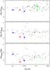 |
Fig. 11 Upper panel: the [Na/Fe] versus [Fe/H] relation in LTE calculations. Middle panel: the relation between sodium, corrected for NLTE effects, and iron abundances. Lower panel: the relation between sodium corrected for NLTE effects, and magnesium as function of [Fe/H]. In the three panels, the symbols are as in Fig. 9. |
5.6.1. Abundances
Both sodium and aluminum abundances are based on strong resonance lines. The D lines at at 5890 Å and 5896 Å were used for Na, the two lines at 3944 Å and 3961 Å for Al. The equivalent widths of Table 6 were used for all stars, except Sex24-72 (see Sect. 4.3). The scandium abundance of Scl07-50 was derived from the two lines at 4247 Å and 4314 Å, since none of the other lines of Table 6 could be detected for this star. For the other stars the two lines at 5031 Å and 5527 Å were used, except for Fnx05-42, where only the line at 5031 Å could be seen. We also used the lines from the blue part with lower S / N for confirmation. After hyperfine structure and scattering corrections the scandium abundances derived from the blue lines and the 5031 Å line respectively, agreed within the errors.
5.6.2. NLTE Effects
Both Na lines used here are resonance lines, they are consequently very sensitive to NLTE effects. Following Baumueller et al. (1998), Cayrel et al. (2004) applied a uniform correction of −0.5 dex to all stars of their sample. But this did not account for a possible dependence of NLTE corrections on atmospheric parameters. Andrievsky et al. (2007) calculated NLTE corrections for a grid of parameters ranging from −2.5 to −4.0 in metallicity, 4500 K to 6350 K in effective temperature and 0.8 to 4.1 in log g (see their Table 2). They applied their results to the samples of giant and turnoff stars of Cayrel et al. (2004); and Bonifacio et al. (2006). We employed their grid using linear interpolations in temperatures and metallicities to estimate the NLTE corrections both for our sample stars and our comparison sample. We calculated the errors on these interpolated corrections as the difference between our values and the ones provided by the closest points in the grid.
The NLTE corrections for a given set of atmospheric parameters also depend on the line strength. Andrievsky et al. (2007) values are therefore only accurate for the given reference equivalent widths. For measured equivalent widths that are significantly different from the reference values, we modified our NLTE corrections according to Fig. 3 of Andrievsky et al. (2007). The Na equivalent widths of Sex11-04 and Sex24-72 are more than 50 mÅ stronger than the highest value covered by Andrievsky et al. (2007), leading to widely uncertain corrections. Therefore we did not consider them. For the same reason, some of the stars in our comparison sample had to be excluded.
Figure 11 displays [Na/Fe]NLTE and [NaNLTE/Mg] as functions of metallicity. The error bars correspond to the quadratic sum of the errors given in Table 7 and the errors in the NLTE corrections mentioned above.
Just as in the analysis of sodium, only the resonance lines of aluminum can be detected at low metallicities, and they are affected by NLTE effects. Andrievsky et al. (2008) calculated NLTE corrections for Al in giants, but for temperatures above 4700 K, implying an extrapolation by up to almost 500 K for some of our stars. Furthermore while they mentioned the dependence of the NLTE corrections on line strength, unfortunately they did not give explicit values. Because NLTE corrections of our Al abundances are too uncertain, we kept the LTE values in Fig. 12.
5.6.3. Analysis
The production of aluminum and sodium is assumed to be bimodal. At low metallicities, in the absence of heavy elements, aluminum is the product of Ne burning in massive stars during their RGB phase, with a very small contribution of C burning, whereas sodium is mainly produced through C burning. These primary processes are only based on the 12C production during the He-burning phase (Woosley & Weaver 1995). It is therefore expected that both [Al/Fe] and [Na/Fe] are constant with [Fe/H]. In metal-rich environments however, with a sufficient amount of neutron rich elements that might act as neutron donors, the yields of Al and Na depend on the neutron excess and their abundances are expected to be metallicity dependent (Woosley & Weaver 1995; Gehren et al. 2006). Andrievsky et al. (2007, 2008) found constant [Na/Fe] and [Al/Fe] values of −0.21 ± 0.13 and −0.06 ± 0.10, respectively.
In the upper panel of Fig. 11, we present the results of our original LTE calculations for Na. In the middle panel of Fig. 11 we show the NLTE values of [Na/Fe] for our EMP stars and the comparison sample. The NLTE corrections together with their uncertainties are reported in Table 5. Within the errors, dSph and Galactic halo stars agree quite well, showing no slope with [Fe/H], as expected at these low metallicities. The largest discrepancies correspond to the largest uncertainties in NLTE corrections and for the Sextans stars, they have low and dispersed abundance ratios, as was also noticed for Mg. Figure 11 shows that the dispersion in sodium abundances perfectly reflects the dispersion in magnesium in Sextans and confirms that the site of production of Na is the same as that of Mg, in dSphs just as in our Galaxy halo.The LTE abundances of aluminum agree with the halo for three of our stars. Only Sex11-04 seems above the bulk of the halo distribution. This is spurious however, given its atmospheric parameters, i.e. [Fe/H] ~ −3 and very low temperature, the non-LTE corrections of this star are expected to be much smaller than for the other stars, which should be substantially moved upward in [Al/Fe] after NLTE corrections (see Fig. 2 of Andrievsky et al. 2008).
NLTE corrections to the sodium D lines according to Andrievsky et al. (2007).
5.7. The iron peak elements
5.7.1. Abundances
The Cr abundance of Scl07-050 was determined from three lines at 4254 Å, 4275 Å, and 4290 Å. In the other stars, we used the line at 5208 Å from the red part of the spectrum and, for the two Sextans stars, two additional lines at 5346 Å and 5410 Å. None of these lines could be detected in Scl07-50. The abundance of the 5208 Å line was derived from spectral synthesis, in order to correct for a blending line.
The manganese abundance of the two Sextans stars was determined from the line at 4824 Å, which was not detected in the other stars. In Fnx05-42 we used two resonance lines of the triplet at ~4030 Å. In Scl07-50, we could use the third line as well. We did not use the resonance lines for the Sextans stars, since the uncertainties of derived abundances were too high.
The Co abundances were determined, when possible, from the three lines at 3995 Å, 4119 Å, and 4121 Å.
The nickel abundance of Scl07-50 was derived from two lines at 3807 Å and 3858 Å. These lines yielded very large errors (> 0.5 dex) for all the other stars and were therefore not considered. An exception was the line at 3858 Å of Fnx05-042, which had somewhat smaller errors (± 0.2−0.3 dex). The line at 5477 Å was detected in all stars, except Scl07-50. For Fnx05-42 the abundances of the blue and the red line agreed very well.
5.7.2. NLTE effects
Several recent publications showed clear evidence for the presence of NLTE effects in the abundances of the iron peak elements. The most important ones were an offset in Mn abundance when derived from the resonance triplet at 4030 Å, (Cayrel et al. 2004; Lai et al. 2008), a trend in [CrI/Fe] with metallicity and effective temperature (Lai et al. 2008), and a deviation of Cr from ionization balance (Sobeck et al. 2007), as well as a difference of [CrI/Fe] between turnoff and giant stars (Bonifacio et al. 2009).
On theoretical grounds, Bergemann & Gehren (2008) and Bergemann et al. (2010) calculated NLTE corrections for manganese and cobalt for a grid of atmospheric parameters and applied their results to 17 stars with metallicities between solar and [Fe/H] = −3.1. Their model atmospheres have higher temperatures and gravities than the stars from our sample, however the main parameter that controls the magnitude of NLTE effects is the metallicity, in the sense that NLTE corrections increase with decreasing [Fe/H]. Both [Co/Fe]NLTE and [Mn/Fe]NLTE are always higher compared to their LTE values. The differences can be up to 0.9 dex for cobalt and ~0.5 dex for manganese.
Whereas the LTE abundances show a downturn of [Mn/Fe] toward lower metallicities, the NLTE abundances are flat with ⟨ [Mn/Fe] ⟩ ~ −0.1 over the whole metallicity range. Unfortunately, no calculations of NLTE effects on [Cr/Fe] exist so far.
To summarize the above discussion, both observations and theory provide very strong evidence for the influence of NLTE effects on the abundances of Co, Cr, and Mn. These effects seem to be particularly large at lower temperatures, for giant stars and when resonance lines of neutral species are used, which are exactly the conditions we meet with our EMP stars. Therefore it is hardly possible to draw any final conclusions from our observed abundances, unless exact calculations of NLTE corrections in the parameter range 4000 K ≤ Teff ≤ 4800 K, 0.5 ≤ log g ≤ 2.0, and −2.5 ≤ [Fe/H] ≤ −4.0 become available.
With this in mind, the somewhat lower cobalt and manganese abundances in Fnx05-042 might be explained considering that it has both very low metallicity and very low gravity, whereas the other stars from our sample are either slightly higher in metallicity (Sextans) or in surface gravity (Sculptor).
5.7.3. Analysis
In the early galaxy evolution, when only massive stars contribute to the chemical enrichment, Co, Cr, and Mn are produced through explosive nucleosynthesis during SN II events. Co is produced in the complete Si burning shell, Cr is mainly produced in the incomplete Si burning shell, and by a small amount also in the complete Si burning region, and Mn is produced exclusively in the incomplete Si burning shell. Abundances of these elements in the galactic halo show a strong odd-even effect (odd nuclei have lower abundances than the even nuclei), which proves to be difficult to be reproduced all at once. Various attempts have been made with standard SN II events (e.g., Woosley & Weaver 1995), zero-metallicity SN II events, including pair-instability SN (e.g., Heger & Woosley 2002), varying the mass-cut (dividing the mass expelled from that falling back onto the remnant) (e.g., Nakamura et al. 1999), hypernovae (i.e. very energetic SNe, with E > 1052 erg) or varying the SN explosion energy (e.g., Nakamura et al. 2001; Umeda & Nomoto 2002, 2005).
The abundances of the iron peak elements are shown in Fig. 13. They generally confirm the results obtained by most of the previous studies of metal-poor stars in the halo: [Co/Fe] is increasing, whereas [Cr/Fe] and [Mn/Fe] are decreasing toward lower metallicities. [Ni/Fe] is flat over the whole metallicity range from −2.5 to −4. The dispersion in [Cr/Fe] is spectacularly small.
Within the limitation due to the NLTE effects, all very and extremely metal-poor stars in systems as different as UFDs and the Milky Way, and including the classical dSphs studied here, show similar abundance ratios among their iron peak elements. This implies that the early enrichment of the galaxy interstellar medium with iron peak elements is independent of the environment.
5.8. The heavy elements
5.8.1. Abundances
The 6142 Å and 6497 Å barium lines are only detected in the two Sextans stars and in Fnx05-42. After spectral synthesis, taking in account the hyperfine splitting, the abundances derived from the equivalent widths were corrected by −0.07 dex, −0.13 dex, and −0.09 dex, for Sex11-04, Sex24-72 and Fnx05-42, respectively. We could only estimate an upper limit on [Ba/H] for Scl07-049. The barium abundance of Scl07-050 is determined from the blue line at 4554.03 Å, which cannot be detected for the other stars, since it is located in the gap between the blue and the red lower CCD chips. Upper limits in [Eu/H] are derived from the region around the 4129 Å line for all stars except Scl07-049. The yttrium abundance can only be measured in Sex11-04, from its line at 4884 Å. For the other stars, only upper limits are estimated. The strontium abundance was determined from the two resonance lines at 4077.7 Å and 4215.5 Å. In Sex24-72 the latter was heavily blended by a CN molecular band and could not be used. The strongest of all Sr lines (at 4077.7 Å in Fnx05-42) has an equivalent width of 231 mÅ and is therefore in the domain where equivalent widths might no longer be appropriate. Thus we did spectral synthesis in order to derive the Sr abundance from this line. All other lines are somewhat weaker, therefore we used their equivalent widths. For the lines with equivalent widths ~200 mÅ however, we tested what difference this would make and found that the abundances derived from synthesis and equivalent widths differed by no more than 0.1 dex, which is small compared to the errors. NLTE effects play a negligible role in our results, because the corrections are below 0.1 dex for both Sr and Ba in our range of effective temperatures (Short & Hauschildt 2006; Mashonkina et al. 2008; Andrievsky et al. 2009).
5.8.2. Analysis
Truran (1981) first demonstrated the r-process origin of barium in very metal-poor stars. Since then two components have been identified: i) the main r-process produces the full range of neutron capture elements; ii) another process called alternatively weak r-process (Ishimaru et al. 2005), LEPP (light element primary process) (Travaglio et al. 2004), or CPR (charged particle reactions) process (Qian & Wasserburg 2007) produces mainly the light (Z < 56 ) neutron capture elements and little or no heavier ones, such as Ba. More recently, Farouqi et al. (2009) have proposed the superpositions of type II supernovae winds with different entropies to reproduce the full range of r-process elements. Barklem et al. (2005) and François et al. (2007) demonstrated the sequential existence of these (at least) two processes in the Milky Way halo stars, by showing that the main r-process dominates, once the heavy elements have been enriched beyond [Ba/H] ~ −2.5. Below this level, another process contributes to the enhancements of Sr as well as Y.
In Fig. 14 we show the relation between [Ba/Fe] and [Sr/Fe] as a function of the metallicity. From our initial comparison sample, we only kept the r-process stars ([Ba/Eu] < 0) in the [Ba/Fe] plot. This required available measurements of the Eu abundance (Lai et al. 2008; François et al. 2007; Honda et al. 2004; Aoki et al. 2005). Similarly for the [Fe/H] ≳ −2. stars in Fornax (Letarte et al. 2010) and Sculptor (Hill et al., in prep.), we required [Ba/Eu] < 0. We also inserted the sample of Milky Way halo stars of Barklem et al. (2005), excluding carbon-rich and [Ba/Eu] > 0 stars as well. There is no difference between metal-poor dwarf and giant stars in Ba abundances (Bonifacio et al. 2009), thus we kept both populations here. We could not distinguish between s- and r-process in Sextans, neither for our present sample, nor for the UFDs. Draco Ba abundances of the stars at [Fe/H] > −2.45 are pure r-process ones (Cohen & Huang 2009). Finally, we included (Shetrone et al. 2001) Ursa Minor and (Shetrone et al. 2003) Carina [Ba/Eu] < 0 stars.
All dSph stars at [Fe/H] < −3 in Fig. 14 are located on top of or very close to the trend of [Ba/Fe] versus [Fe/H] defined by the Galactic halo. Above this metallicity and below [Fe/H] ~ −2., the least massive dSph galaxies (here represented by stars in Coma Berenices, Ursa Major, Draco) are preferentially found in the [Ba/Fe] < 0 regime. Sextans however, like its sibling higher mass galaxies Scl and Fnx in the EMP regime, seems to lie on the galactic halo trend (and dispersion). At [Fe/H] > −2.5, the smallest dSphs keep very low Ba abundances, while the Galactic halo stars have already reduced their dispersion and cluster around [Ba/Fe] solar. Carina, Sextans, Draco and even Ursa Minor definitely reach [Ba/Fe] ~ 0 at [Fe/H] ~ −2., with little dispersion, while fainter galaxies, corresponding to MV < −8 (Simon & Geha 2007), do not. This means that among the galaxies that are fainter than Sextans, some will finally increase their Ba abundance sufficiently to catch up with the solar Galactic halo level.
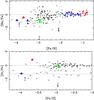 |
Fig. 14 Abundance ratios [Ba/Fe] and [Sr/Fe] as a function of [Fe/H]. General symbols are as in Fig. 9. From our initial comparison sample, we only keep the r-process only stars in the [Ba/Fe] plot. This requires to have measurements of the Eu abundance. This was possible with Lai et al. (2008); François et al. (2007); Honda et al. (2004); Aoki et al. (2005). We also inserted the sample of Milky Way halo stars of Barklem et al. (2005), similarly excluding carbon-rich and [Ba/Eu] > 0 (s-process enriched stars). As to the UFDs, we use the analysis and upper limits in [Ba/Fe] of Koch et al. (2008b) on Hercules (plus sign). In the case of Scl07-49, we could only estimate an upper limit for [Ba/H] in that we indicate with an arrow. Missing the blue part of its spectrum we could not measure its abundance in SrII. Data from Shetrone et al. (2001) in Ursa Minor are identified with small six-branches stars and. The Carina stars (crosses) at [Fe/H] > −2.5 are taken from Shetrone et al. (2003). The dotted line at [Sr/Fe] = −1.23 corresponds to the mean abundance ratio of the smallest dwarfs (fainter than Draco) and to the level of the Galatic halo stars for [Fe/H] ≤ −3.7. |
Galactic mass is a crucial parameter to sustain the explosions of supernovae (Ferrara & Tolstoy 2000), but also to shape the homogeneity of the interstellar medium and the frequency at which gas can cool and form stars (Revaz et al. 2009). In low-mass systems gas is expelled easily, while it is retained in more massive ones, leading to a more complete chemical evolution and homogeneity. Barium is the first chemical element, which seems to provide clear evidence for differential early evolution of the dSphs depending on their mass. Moreover, Fig.14 provides clues on the site of production of the main r-process, in particular by comparison with the α-elements which are produced in a universal way below [Fe/H] ~ −2.5 (Figs. 10 and 9).
Models should be generated to investigate whether low-mass systems could resist the explosions of a few high-mass supernovae but not multiple lower mass ones, thereby loosing the main r-process elements produced in O-Ne-Mg core collapse of 8−10 stars (Wanajo et al. 2003). Alternatively, it is not straightforward to reconcile that the neutron winds of core-collapse SNe II (Qian & Wasserburg 2007; Farouqi et al. 2009) would be expelled from the galaxy bodies, while leaving a normal enrichment in the α elements but a depletion in r-process ones. The work of Cescutti et al. (2006) provides another way to tackle the question of the enrichment in Ba with time or [Fe/H]. The dispersion in [Ba/Fe] observed at [Fe/H] ≲ −3.5 or below [Fe/H] ≤ −2 for the faint dSphs is of the order 1dex. This corresponds to the intrinsic spread predicted by Cescutti et al. (2006)’s model 1, in which barium is produced by 15−30 massive stars. Their stellar yields in barium is increasing with decreasing stellar masses, by a factor ~1000 between 30 and 12 , but only by a factor 10 between 30 and 15 . At [Fe/H] = −3.5 their lightest stellar mass star dying is ~15 . It is likely the minimum stellar mass that can enrich the faintest dSphs. For the more massive ones, the full range of 12−30 provides a good fit to the data.
For [Sr/Fe], the distinction between low- and high- mass galaxies is clearer. Our comparison sample is that of Sect. 5.1 to which we added the measurements of Barklem et al. (2005) with no restriction on [Ba/Eu]. Galaxies similar to Draco or fainter have a constant [Sr/Fe] with a mean [Sr/Fe] = −1.23 and a dispersion of 0.29 dex, corresponding to the abundance ratio of the Milky Way halo stars at [Fe/H] ≤ −3.5, but up to more than one dex below the level of the Milky Way at [Fe/H] > −2.6. Conversely, Scl07-50 and the two Sextans stars in our sample perfectly follow the galactic halo trend in [Sr/Fe], while Fnx05-42 displays a higher [Sr/Fe] value [Sr/Fe] ~ +0.87, yet still within the 2σ dispersion of Barklem et al. (2005) and echoing its relatively high barium content.
While different star formation histories lead to different evolution in the strontium and barium enrichements, it is remarkable that in the earliest stages of the galaxy evolution, here characterized by [Fe/H] below −3.5 or so, all galaxies, from the UFDs to the massive Milky Way, produce the same amount of r-process elements.
Figure 15 sheds light on the relation between primary and secondary r-process. François et al. (2007) precisely described that although Milky Way halo stars show a decrease in [Sr/Fe] and increased scatter below [Fe/H] of −3 (similarly to [Ba/Fe]), a strong relationship of [Sr/Ba] as a function of [Ba/H] is hidden in this dispersion. Indeed, below [Ba/H] = −3 [Sr/Ba] increases from a solar ratio reaching up to +1 dex at [Ba/H] = −4. This is the strongest evidence to date for the weak r-process to arise earlier in the Milky Way evolution than the main r-process. Below this, [Sr/Ba] scatters down back to solar values again around [Ba/H] = −5. All four stars for which we could measure Sr and Ba follow the [Sr/Ba] Galactic trend (Fig. 15), suggesting a constant and universal ratio between the processes delivering heavy and light r-process elements. Nevertheless, further investigation is clearly needed to clarify why some of the ultra faint dwarfs, such as Coma Berenices and Ursa Major II seem to follow the same relation between strontium and barium as the Milky Way halo and the classical dSph stars, while others, such as Boötes or Draco, are clear outsiders, showing lower [Sr/H] than expected from their barium content.
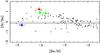 |
Fig. 15 [Sr/Ba] versus [Ba/H] for the comparison sample (see Fig. 14 and for the EMP stars of this work. Symbols as in Fig. 9. The plain line indicates the solar r-process [Sr/Ba], as derived by Simmerer et al. (2004). |
6. Summary and concluding remarks
We analyzed high-resolution VLT/UVES spectra of five metal-poor candidates in three different dwarf spheroidal galaxies, Sextans, Fornax, and Sculptor. The abundances of 15 chemical elements were derived.
All stars from our sample have metallicities around or below −3. This significantly increases the total number of extremely metal-poor stars observed in dwarf galaxies, placing their metallicity floor at a level comparable with the Milky Way Halo. Moreover our sample contains the most metal poor star ever observed in a dwarf galaxy, Scl07-50 with [Fe/H] = −3.96 ± 0.06.
The analysis of the chemical composition of our sample stars and the comparison with the Milky Way halo and other classical and ultra-faint dwarf galaxies, allowed us unprecedented insights in the earliest chemical enrichment of these galaxies. Our main results are the following:
-
We showed that all our stars have undergone some degree of internal mixing, consistent with their advanced evolutionary stages. Taking into consideration mixing-induced carbon depletion, one Sextans star in our sample, Sex24-72, must be considered as carbon-enhanced. This carbon enhancement most likely reflects the pristine property of the ISM rather than mass transfer from an AGB companion. Similar moderately carbon-rich high-luminosity stars had been previously identified in Draco and Ursa MajorII, while they do not exist in the Milky Way halo. Interestingly, we found evidence for inhomogeneities in the early ISM in Sextans: the carbon abundances of our two Sextans stars are very different, despite their similar metallicities, temperatures, gravities, and abundance ratios for all the other elements.
-
We showed that below [Fe/H] = −3, the abundances of the α-elements show no major difference between the various galaxies in our comparison sample, from small to massive systems. Similarly, the abundances of the iron peak elements, aluminum and sodium in dwarf galaxies follow the trends with metallicity seen in the Milky Way halo. This suggests that the conditions of nucleosynthesis and of early enrichment of the interstellar medium are universal for these elements, i.e., independent on the properties of the host galaxy.
-
Below [Fe/H] ~ −3.5 all galaxies have similar low barium and strontium contents. Above this metallicity, galaxies fainter than Draco have [Sr/Fe] ~ −1.23 and [Ba/Fe] ~ −1, while the more massive ones increase their r-process chemical abundances, eventually reaching the solar level observed in the Milky Way. Despite this variation with galaxy mass, there is some evidence for a constant ratio between the “weak” and “main” r-processes, although in some cases, such as Boötes, the Sr content is lower than expected from the abundance in Ba. This issue definitely deserves follow-up.
Online material
Online material
Linelist, equivalent widths and scattering corrections. These corrections are subtracted from the original abundances calculated with calrai. The exponents have the following meanings: (1) Equivalent widths are not used, abundances are determined from synthesis instead; (2) Hyperfine structure was taken into account. (3) Lines are not used, due to very high uncertainties (e.g. blendlines, low S / N etc.)
Abundances.
DAOSPEC has been written by P. Stetson for the Dominion Astrophysical Observatory of the Herzberg Institute of Astrophysics, National Research Council, Canada.
Acknowledgments
This publication makes use of data products from the Two Micron All Sky Survey, which is a joint project of the University of Massachusetts and the Infrared Processing and Analysis Center/California Institute of Technology, funded by the National Aeronautics and Space Administration and the National Science Foundation.
We thank the VISTA commissioning team for providing J, Ks photometry of this object which was observed during the commissioning process.
The Hobby-Eberly Telescope (HET) is a joint project of the University of Texas at Austin, the Pennsylvania State University, Stanford University, Ludwig-Maximilians-Universitat Munchen, and Georg-August-Universitat Gottingen. The HET is named in honor of its principal benefactors, William P. Hobby and Robert E. Eberly. MS would like to thank the NSF for support for the HET observations through AST-0306884.
References
- Alonso, A., Arribas, S., & Martínez-Roger, C. 1999, A&AS, 140, 261 [NASA ADS] [CrossRef] [EDP Sciences] [Google Scholar]
- Alvarez, R., & Plez, B. 1998, A&A, 330, 1109 [NASA ADS] [Google Scholar]
- Anders, E., & Grevesse, N. 1989, Geochim. Cosmochim. Acta, 53, 197 [Google Scholar]
- Andrievsky, S. M., Spite, M., Korotin, S. A., et al. 2007, A&A, 464, 1081 [NASA ADS] [CrossRef] [EDP Sciences] [Google Scholar]
- Andrievsky, S. M., Spite, M., Korotin, S. A., et al. 2008, A&A, 481, 481 [NASA ADS] [CrossRef] [EDP Sciences] [Google Scholar]
- Andrievsky, S. M., Spite, M., Korotin, S. A., et al. 2009, A&A, 494, 1083 [NASA ADS] [CrossRef] [EDP Sciences] [Google Scholar]
- Aoki, W., Honda, S., Beers, T. C., et al. 2005, ApJ, 632, 611 [NASA ADS] [CrossRef] [Google Scholar]
- Aoki, W., Beers, T. C., Christlieb, N., et al. 2007, ApJ, 655, 492 [NASA ADS] [CrossRef] [Google Scholar]
- Aoki, W., Arimoto, N., Sadakane, K., et al. 2009, A&A, 502, 569 [NASA ADS] [CrossRef] [EDP Sciences] [Google Scholar]
- Asplund, M. 2005, ARA&A, 43, 481 [NASA ADS] [CrossRef] [Google Scholar]
- Barklem, P. S., Christlieb, N., Beers, T. C., et al. 2005, A&A, 439, 129 [NASA ADS] [CrossRef] [EDP Sciences] [Google Scholar]
- Battaglia, G., Tolstoy, E., Helmi, A., et al. 2006, A&A, 459, 423 [NASA ADS] [CrossRef] [EDP Sciences] [Google Scholar]
- Battaglia, G., Irwin, M., Tolstoy, E., et al. 2008, MNRAS, 383, 183 [Google Scholar]
- Battaglia, G. Tolstoy, E. Helmi, A., et al. 2010 e-prints [arXiv:1009.4857] [Google Scholar]
- Baumueller, D., Butler, K., & Gehren, T. 1998, A&A, 338, 637 [NASA ADS] [Google Scholar]
- Beers, T. C., & Christlieb, N. 2005, ARA&A, 43, 531 [NASA ADS] [CrossRef] [Google Scholar]
- Bergemann, M., & Gehren, T. 2008, A&A, 492, 823 [NASA ADS] [CrossRef] [EDP Sciences] [Google Scholar]
- Bergemann, M., Pickering, J. C., & Gehren, T. 2010, MNRAS, 401, 1334 [NASA ADS] [CrossRef] [Google Scholar]
- Bersier, D., & Wood, P. R. 2002, AJ, 123, 840 [NASA ADS] [CrossRef] [Google Scholar]
- Bisterzo, S., Gallino, R., Straniero, O., Cristallo, S., & Käppeler, F. 2010, MNRAS, 404, 1529 [NASA ADS] [Google Scholar]
- Bonifacio, P., Zaggia, S., Sbordone, L., et al. 2006, Abundances in Sagittarius Stars, ed. S. Randich, & L. Pasquini, 232 [Google Scholar]
- Bonifacio, P., Spite, M., Cayrel, R., et al. 2009, A&A, 501, 519 [NASA ADS] [CrossRef] [EDP Sciences] [Google Scholar]
- Buonanno, R., Corsi, C. E., Castellani, M., et al. 1999, AJ, 118, 1671 [NASA ADS] [CrossRef] [Google Scholar]
- Carretta, E., Gratton, R., Cohen, J. G., Beers, T. C., & Christlieb, N. 2002, AJ, 124, 481 [NASA ADS] [CrossRef] [Google Scholar]
- Cayrel, R. 1988, The Impact of Very High S/N Spectroscopy on Stellar Physics, ed. G. Cayrel de Strobel, & M. Spite, in IAU Symp., 132, 345 [Google Scholar]
- Cayrel, R., Perrin, M., Barbuy, B., & Buser, R. 1991, A&A, 247, 108 [NASA ADS] [Google Scholar]
- Cayrel, R., Depagne, E., Spite, M., et al. 2004, A&A, 416, 1117 [NASA ADS] [CrossRef] [EDP Sciences] [Google Scholar]
- Cescutti, G., François, P., Matteucci, F., Cayrel, R., & Spite, M. 2006, A&A, 448, 557 [NASA ADS] [CrossRef] [EDP Sciences] [Google Scholar]
- Christlieb, N., Bessell, M. S., Beers, T. C., et al. 2002, Nature, 419, 904 [NASA ADS] [CrossRef] [PubMed] [Google Scholar]
- Cohen, J. G., & Huang, W. 2009, ApJ, 701, 1053 [NASA ADS] [CrossRef] [Google Scholar]
- Cohen, J. G., Christlieb, N., McWilliam, A., et al. 2004, ApJ, 612, 1107 [NASA ADS] [CrossRef] [Google Scholar]
- Cohen, J. G., McWilliam, A., Shectman, S., et al. 2006, AJ, 132, 137 [NASA ADS] [CrossRef] [Google Scholar]
- Cohen, J. G., Christlieb, N., McWilliam, A., et al. 2008, ApJ, 672, 320 [NASA ADS] [CrossRef] [Google Scholar]
- Coleman, M. G., & de Jong, J. T. A. 2008, ApJ, 685, 933 [NASA ADS] [CrossRef] [Google Scholar]
- Cristallo, S., Straniero, O., Gallino, R., et al. 2009, ApJ, 696, 797 [NASA ADS] [CrossRef] [Google Scholar]
- Denissenkov, P. A., & Pinsonneault, M. 2008, ApJ, 679, 1541 [NASA ADS] [CrossRef] [Google Scholar]
- Eggleton, P. P., Dearborn, D. S. P., & Lattanzio, J. C. 2008, ApJ, 677, 581 [NASA ADS] [CrossRef] [Google Scholar]
- Farouqi, K., Kratz, K., Mashonkina, L. I., et al. 2009, ApJ, 694, L49 [NASA ADS] [CrossRef] [Google Scholar]
- Ferrara, A., & Tolstoy, E. 2000, MNRAS, 313, 291 [NASA ADS] [CrossRef] [Google Scholar]
- François, P., Depagne, E., Hill, V., et al. 2007, A&A, 476, 935 [NASA ADS] [CrossRef] [EDP Sciences] [Google Scholar]
- Frebel, A., Kirby, E. N., & Simon, J. D. 2010a, Nature, 464, 72 [NASA ADS] [CrossRef] [Google Scholar]
- Frebel, A., Simon, J. D., Geha, M., & Willman, B. 2010b, ApJ, 708, 560 [NASA ADS] [CrossRef] [Google Scholar]
- Fulbright, J. P., Rich, R. M., & Castro, S. 2004, ApJ, 612, 447 [NASA ADS] [CrossRef] [Google Scholar]
- Fusi Pecci, F., Ferraro, F. R., Crocker, D. A., Rood, R. T., & Buonanno, R. 1990, A&A, 238, 95 [NASA ADS] [Google Scholar]
- Gehren, T., Shi, J. R., Zhang, H. W., Zhao, G., & Korn, A. J. 2006, A&A, 451, 1065 [NASA ADS] [CrossRef] [EDP Sciences] [Google Scholar]
- Gratton, R. G., Sneden, C., Carretta, E., & Bragaglia, A. 2000, A&A, 354, 169 [NASA ADS] [Google Scholar]
- Grevesse, N., & Sauval, A. J. 1998, Space Sci. Rev., 85, 161 [NASA ADS] [CrossRef] [Google Scholar]
- Gustafsson, B., Bell, R. A., Eriksson, K., & Nordlund, A. 1975, A&A, 42, 407 [NASA ADS] [Google Scholar]
- Gustafsson, B., Edvardsson, B., Eriksson, K., et al. 2003, in Stellar Atmosphere Modeling, ed. I. Hubeny, D. Mihalas, & K. Werner, ASP Conf. Ser., 288, 331 [Google Scholar]
- Gustafsson, B., Edvardsson, B., Eriksson, K., et al. 2008, A&A, 486, 951 [NASA ADS] [CrossRef] [EDP Sciences] [Google Scholar]
- Heger, A., & Woosley, S. E. 2002, ApJ, 567, 532 [NASA ADS] [CrossRef] [Google Scholar]
- Heiter, U., & Eriksson, K. 2006, A&A, 452, 1039 [NASA ADS] [CrossRef] [EDP Sciences] [Google Scholar]
- Helmi, A., Irwin, M. J., Tolstoy, E., et al. 2006, ApJ, 651, L121 [NASA ADS] [CrossRef] [Google Scholar]
- Hill, V. 2010, in IAU Symposium, ed. K. Cunha, M. Spite, & B. Barbuy, IAU Symp., 265, 219 [Google Scholar]
- Honda, S., Aoki, W., Kajino, T., et al. 2004, ApJ, 607, 474 [NASA ADS] [CrossRef] [Google Scholar]
- Hurley-Keller, D., Mateo, M., & Grebel, E. K. 1999, ApJ, 523, L25 [NASA ADS] [CrossRef] [Google Scholar]
- Ishimaru, Y., Wanajo, S., Aoki, W., Ryan, S. G., & Prantzos, N. 2005, Nucl. Phys. A, 758, 603 [NASA ADS] [CrossRef] [Google Scholar]
- Karachentsev, I. D., Karachentseva, V. E., Huchtmeier, W. K., & Makarov, D. I. 2004, AJ, 127, 2031 [Google Scholar]
- Karakas, A. I. 2010, MNRAS, 403, 1413 [NASA ADS] [CrossRef] [Google Scholar]
- Kirby, E. N., Simon, J. D., Geha, M., Guhathakurta, P., & Frebel, A. 2008, ApJ, 685, L43 [NASA ADS] [CrossRef] [Google Scholar]
- Koch, A., Grebel, E. K., Gilmore, G. F., et al. 2008a, AJ, 135, 1580 [NASA ADS] [CrossRef] [Google Scholar]
- Koch, A., McWilliam, A., Grebel, E. K., Zucker, D. B., & Belokurov, V. 2008b, ApJ, 688, L13 [NASA ADS] [CrossRef] [Google Scholar]
- Lai, D. K., Bolte, M., Johnson, J. A., et al. 2008, ApJ, 681, 1524 [NASA ADS] [CrossRef] [Google Scholar]
- Lee, M. G., Park, H. S., Park, J.-H., et al. 2003, AJ, 126, 2840 [NASA ADS] [CrossRef] [Google Scholar]
- Letarte, B., Hill, V., Tolstoy, E., et al. 2010, A&A, 523, A17 [NASA ADS] [CrossRef] [EDP Sciences] [Google Scholar]
- Magain, P. 1984, A&A, 134, 189 [NASA ADS] [Google Scholar]
- Majewski, S. R., Siegel, M. H., Patterson, R. J., & Rood, R. T. 1999, ApJ, 520, L33 [NASA ADS] [CrossRef] [MathSciNet] [Google Scholar]
- Mashonkina, L., Zhao, G., Gehren, T., et al. 2008, A&A, 478, 529 [NASA ADS] [CrossRef] [EDP Sciences] [Google Scholar]
- McWilliam, A., Preston, G. W., Sneden, C., & Shectman, S. 1995, AJ, 109, 2736 [NASA ADS] [CrossRef] [Google Scholar]
- Meynet, G., Ekström, S., & Maeder, A. 2006, A&A, 447, 623 [NASA ADS] [CrossRef] [EDP Sciences] [Google Scholar]
- Monkiewicz, J., Mould, J. R., Gallagher, III, J. S., et al. 1999, PASP, 111, 1392 [NASA ADS] [CrossRef] [Google Scholar]
- Nakamura, T., Umeda, H., Nomoto, K., Thielemann, F., & Burrows, A. 1999, ApJ, 517, 193 [NASA ADS] [CrossRef] [Google Scholar]
- Nakamura, T., Umeda, H., Iwamoto, K., et al. 2001, ApJ, 555, 880 [NASA ADS] [CrossRef] [Google Scholar]
- Norris, J. E., Yong, D., Gilmore, G., & Wyse, R. F. G. 2010, ApJ, 711, 350 [NASA ADS] [CrossRef] [Google Scholar]
- Prochaska, J. X., Naumov, S. O., Carney, B. W., McWilliam, A., & Wolfe, A. M. 2000, AJ, 120, 2513 [NASA ADS] [CrossRef] [Google Scholar]
- Qian, Y., & Wasserburg, G. J. 2007, Phys. Rep., 442, 237 [NASA ADS] [CrossRef] [Google Scholar]
- Ramírez, I., & Meléndez, J. 2005, ApJ, 626, 465 [Google Scholar]
- Ramsey, L. W., Adams, M. T., Barnes, T. G., et al. 1998, in SPIE Conf. Ser. 3352, ed. L. M. Stepp, 34 [Google Scholar]
- Revaz, Y., Jablonka, P., Sawala, T., et al. 2009, A&A, 501, 189 [NASA ADS] [CrossRef] [EDP Sciences] [Google Scholar]
- Ryan, S. G., Norris, J. E., & Beers, T. C. 1996, ApJ, 471, 254 [NASA ADS] [CrossRef] [Google Scholar]
- Schlegel, D. J., Finkbeiner, D. P., & Davis, M. 1998, ApJ, 500, 525 [NASA ADS] [CrossRef] [Google Scholar]
- Shetrone, M. D., Côté, P., & Sargent, W. L. W. 2001, ApJ, 548, 592 [NASA ADS] [CrossRef] [Google Scholar]
- Shetrone, M., Venn, K. A., Tolstoy, E., et al. 2003, AJ, 125, 684 [NASA ADS] [CrossRef] [Google Scholar]
- Short, C. I., & Hauschildt, P. H. 2006, ApJ, 641, 494 [NASA ADS] [CrossRef] [Google Scholar]
- Simmerer, J., Sneden, C., Cowan, J. J., et al. 2004, ApJ, 617, 1091 [NASA ADS] [CrossRef] [Google Scholar]
- Simon, J. D., & Geha, M. 2007, ApJ, 670, 313 [NASA ADS] [CrossRef] [Google Scholar]
- Simon, J. D., Frebel, A., McWilliam, A., Kirby, E. N., & Thompson, I. B. 2010, ApJ, 716, 446 [NASA ADS] [CrossRef] [Google Scholar]
- Skrutskie, M. F., Cutri, R. M., Stiening, R., et al. 2006, AJ, 131, 1163 [NASA ADS] [CrossRef] [Google Scholar]
- Sobeck, J. S., Lawler, J. E., & Sneden, C. 2007, ApJ, 667, 1267 [NASA ADS] [CrossRef] [Google Scholar]
- Spite, M. 1967, Ann. Astrophys., 30, 211 [Google Scholar]
- Spite, M., Cayrel, R., Plez, B., et al. 2005, A&A, 430, 655 [NASA ADS] [CrossRef] [EDP Sciences] [Google Scholar]
- Spite, M., Cayrel, R., Hill, V., et al. 2006, A&A, 455, 291 [NASA ADS] [CrossRef] [EDP Sciences] [Google Scholar]
- Stancliffe, R. J., Church, R. P., Angelou, G. C., & Lattanzio, J. C. 2009, MNRAS, 396, 2313 [Google Scholar]
- Starkenburg, E., Hill, V., Tolstoy, E., et al. 2010, A&A, 513, A34 [NASA ADS] [CrossRef] [EDP Sciences] [Google Scholar]
- Stetson, P. B., Hesser, J. E., & Smecker-Hane, T. A. 1998, PASP, 110, 533 [NASA ADS] [CrossRef] [Google Scholar]
- Suda, T., & Fujimoto, M. Y. 2010, MNRAS, 405, 177 [NASA ADS] [Google Scholar]
- Tolstoy, E. 2010, in IAU Symp. 262, ed. G. Bruzual & S. Charlot, 119 [Google Scholar]
- Tolstoy, E., Irwin, M. J., Helmi, A., et al. 2004, ApJ, 617, L119 [NASA ADS] [CrossRef] [Google Scholar]
- Tolstoy, E., Hill, V., & Tosi, M. 2009, ARA&A, 47, 371 [NASA ADS] [CrossRef] [Google Scholar]
- Travaglio, C., Gallino, R., Arnone, E., et al. 2004, ApJ, 601, 864 [NASA ADS] [CrossRef] [Google Scholar]
- Truran, J. W. 1981, A&A, 97, 391 [NASA ADS] [Google Scholar]
- Tull, R. G. 1998, in Optical Astronomical Instrumentation, Sandro D’Odorico, SPIE Conf. 3355, ed. S. D’Odorico, 387 [Google Scholar]
- Umeda, H., & Nomoto, K. 2002, ApJ, 565, 385 [NASA ADS] [CrossRef] [Google Scholar]
- Umeda, H., & Nomoto, K. 2005, ApJ, 619, 427 [NASA ADS] [CrossRef] [Google Scholar]
- Venn, K. A., Irwin, M., Shetrone, M. D., et al. 2004, AJ, 128, 1177 [NASA ADS] [CrossRef] [Google Scholar]
- Wanajo, S., Tamamura, M., Itoh, N., et al. 2003, ApJ, 593, 968 [NASA ADS] [CrossRef] [Google Scholar]
- Woosley, S. E., & Weaver, T. A. 1986, ARA&A, 24, 205 [NASA ADS] [CrossRef] [Google Scholar]
- Woosley, S. E., & Weaver, T. A. 1995, ApJS, 101, 181 [NASA ADS] [CrossRef] [Google Scholar]
All Tables
Log of observations. The exposure times are given for the blue and red arms of UVES.
Linelist, equivalent widths and scattering corrections. These corrections are subtracted from the original abundances calculated with calrai. The exponents have the following meanings: (1) Equivalent widths are not used, abundances are determined from synthesis instead; (2) Hyperfine structure was taken into account. (3) Lines are not used, due to very high uncertainties (e.g. blendlines, low S / N etc.)
All Figures
|
Fig. 1 Spectra of our five sample stars, ranked by decreasing value of [Fe/H], in the region of MgI. For comparison two Milky Way halo stars are included, HD 122563 and CD −38 245, at [Fe/H] = −2.8 and [Fe/H] = −4.19, respectively. |
| In the text | |
|
Fig. 2 Reddening corrected color − magnitude diagrams of Sextans, Fornax, and Sculptor for our galaxy members selected from their spectra in the CaT region. |
| In the text | |
|
Fig. 3 Lower panel: the differences in abundances derived assuming a pure absorption source function and when a scattering term is introduced. All calculations are done with turbospectrum. All lines are considered and are shown at their wavelengths. Black points trace Fnx05-42, blue stands for the 2 Sextans stars, red for Scl07-49 and green for Scl07-50. Upper panel: [FeI/H] when scattering is properly taken into account. There is no trend of abundance with wavelength, while there was a clear increase at bluer wavelengths before correction. |
| In the text | |
|
Fig. 4 DART dSph targets are in color: Sextans(Green) Scl(Blue) Fnx (Red). Large triangles identify the 5 stars analyzed here, while small triangles indicate stars in earlier publications (Letarte et al. 2010; Aoki et al. 2009; Shetrone et al. 2001; Frebel et al. 2010a). Open squares: UFDs, Carina and Draco (Fulbright et al. 2004; Koch et al. 2008a,b; Frebel et al. 2010b; Cohen & Huang 2009; Norris et al. 2010; Simon et al. 2010). The Milky Way halo stars are represented by circles; open circles are unmixed RGBs and filled circles mixed RGBs (Cayrel et al. 2004; Cohen et al. 2008; Aoki et al. 2005; Spite et al. 2005; Aoki et al. 2007; Cohen et al. 2006; Lai et al. 2008; Honda et al. 2004). |
| In the text | |
|
Fig. 5 The comparison of the equivalent widths of Scl05-50 ([Fe/H] = −3.96) and the Milky Way halo star CD−38 245 ([Fe/H] = −4.19). The dashed lined follows the mean ~20 mÅ difference between the equivalent widths of the two stars. |
| In the text | |
|
Fig. 6 Comparison for our sample stars between [Fe/H] from high resolution UVES measurements ([Fe/H]HR) and that from the CaT with the calibration of Battaglia et al. (2008) ([Fe/H]LR), as filled circles. For Sex24-72 HET/HRS spectroscopy at R ~ 18000 is used because CaT data are not available. Blue stands for the Sculptor’s stars, red for the Fornax’ star, and green is for Sextans’s ones. The CaT metallicity determined with the new calibration of Starkenburg et al. (2010) for low metallicities are shown as open circles. Crosses provide the same comparison at [Fe/H] > −2.5, where the classical (old) CaT calibration is robust. |
| In the text | |
|
Fig. 7 Synthesis of the molecular CH band at 4323 Å of Sex24-72. The crosses are the observed spectrum, the red line corresponds to the synthetic spectrum with [C/Fe] = 0.0, the green lines are for [C/Fe] = ± 0.5, the blue line is for [C/Fe] = 1.0, and the black line for the complete absence of C. |
| In the text | |
|
Fig. 8 DART dSph targets are in colored triangles: Sextans(Green) Scl(Blue) Fnx (Red). Other symbols are squares (Ursa MajorII), triangles (Coma Berenices), diamonds (Draco), star (Boötes) (Fulbright et al. 2004; Koch et al. 2008a; Frebel et al. 2010b; Cohen & Huang 2009; Norris et al. 2010). Only mixed Milky Way halo stars (black dots) are considered (Cayrel et al. 2004; Cohen et al. 2008; Honda et al. 2004; Aoki et al. 2005, 2007; Cohen et al. 2006; Lai et al. 2008). The dashed line delineates the regions in which they are observed. |
| In the text | |
|
Fig. 9 DART dSph targets are in colored triangles: Sextans(Green) Scl(Blue) Fnx (Red). Large symbols stand for the sample stars of this work, small ones stand for earlier works and publications (Hill et al., in prep.; Letarte et al. 2010; Frebel et al. 2010a; Aoki et al. 2009; Shetrone et al. 2001). Other symbols are squares (Ursa MajorII, Frebel et al. 2010b), triangles (Coma Berenices, Frebel et al. 2010b), diamonds (Draco, Shetrone et al. 2001; Fulbright et al. 2004; Cohen & Huang 2009), star (Boötes, Norris et al. 2010), cross (Carina, Shetrone et al. 2003; Koch et al. 2008a), and circle (Leo IV, Simon et al. 2010). All Milky Way halo stars from our comparison sample are considered (black dots) Cayrel et al. (2004); Honda et al. (2004); Aoki et al. (2005, 2007); Cohen et al. (2006, 2008); Lai et al. (2008). For the purpose of this figure, Venn et al. (2004)’s compilation was added at [Fe/H] ≥ −2.5. |
| In the text | |
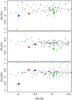 |
Fig. 10 Variation of the α elements with [Fe/H]. Symbols are as in Fig. 9. |
| In the text | |
|
Fig. 11 Upper panel: the [Na/Fe] versus [Fe/H] relation in LTE calculations. Middle panel: the relation between sodium, corrected for NLTE effects, and iron abundances. Lower panel: the relation between sodium corrected for NLTE effects, and magnesium as function of [Fe/H]. In the three panels, the symbols are as in Fig. 9. |
| In the text | |
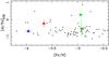 |
Fig. 12 Relation between aluminum and iron. Symbols as in Fig. 9. |
| In the text | |
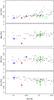 |
Fig. 13 Iron peak elements. Symbols as in Fig. 9. |
| In the text | |
|
Fig. 14 Abundance ratios [Ba/Fe] and [Sr/Fe] as a function of [Fe/H]. General symbols are as in Fig. 9. From our initial comparison sample, we only keep the r-process only stars in the [Ba/Fe] plot. This requires to have measurements of the Eu abundance. This was possible with Lai et al. (2008); François et al. (2007); Honda et al. (2004); Aoki et al. (2005). We also inserted the sample of Milky Way halo stars of Barklem et al. (2005), similarly excluding carbon-rich and [Ba/Eu] > 0 (s-process enriched stars). As to the UFDs, we use the analysis and upper limits in [Ba/Fe] of Koch et al. (2008b) on Hercules (plus sign). In the case of Scl07-49, we could only estimate an upper limit for [Ba/H] in that we indicate with an arrow. Missing the blue part of its spectrum we could not measure its abundance in SrII. Data from Shetrone et al. (2001) in Ursa Minor are identified with small six-branches stars and. The Carina stars (crosses) at [Fe/H] > −2.5 are taken from Shetrone et al. (2003). The dotted line at [Sr/Fe] = −1.23 corresponds to the mean abundance ratio of the smallest dwarfs (fainter than Draco) and to the level of the Galatic halo stars for [Fe/H] ≤ −3.7. |
| In the text | |
|
Fig. 15 [Sr/Ba] versus [Ba/H] for the comparison sample (see Fig. 14 and for the EMP stars of this work. Symbols as in Fig. 9. The plain line indicates the solar r-process [Sr/Ba], as derived by Simmerer et al. (2004). |
| In the text | |
Current usage metrics show cumulative count of Article Views (full-text article views including HTML views, PDF and ePub downloads, according to the available data) and Abstracts Views on Vision4Press platform.
Data correspond to usage on the plateform after 2015. The current usage metrics is available 48-96 hours after online publication and is updated daily on week days.
Initial download of the metrics may take a while.