| Issue |
A&A
Volume 523, November-December 2010
|
|
|---|---|---|
| Article Number | A24 | |
| Number of page(s) | 15 | |
| Section | Stellar structure and evolution | |
| DOI | https://doi.org/10.1051/0004-6361/201014970 | |
| Published online | 11 November 2010 | |
The barium isotopic mixture for the metal-poor subgiant star HD 140283⋆
1
Centre for Astrophysics Research, School of Physics, Astronomy &
Mathematics, University of Hertfordshire, College Lane, Hatfield
Hertfordshire
AL10 9AB
UK
e-mail: This email address is being protected from spambots. You need JavaScript enabled to view it.
; This email address is being protected from spambots. You need JavaScript enabled to view it.
2
Department of Astronomy, PO Box 400325, University of
Virginia, Charlottesville, VA
22904-4325,
USA
e-mail: This email address is being protected from spambots. You need JavaScript enabled to view it.
3
National Astronomical Observatory, Mitika, Tokyo
181-8588,
Japan
e-mail: This email address is being protected from spambots. You need JavaScript enabled to view it.
Received:
10
May
2010
Accepted:
20
August
2010
Abstract
Context. Current theory regarding heavy element nucleosynthesis in metal-poor environments states that the r-process would be dominant. The star HD 140283 has been the subject of debate after it appeared in some studies to be dominated by the s-process.
Aims. We provide an independent measure of the Ba isotope mixture using an extremely high quality spectrum and an extensive χ2 analysis.
Methods. We have acquired a very high resolution (R ≡ λ/Δλ = 95000), very high signal-to-noise (S / N = 1110 around 4554 Å, as calculated in IRAF) spectrum of HD 140283. We exploit hyperfine splitting of the Ba ii 4554 Å and 4934 Å resonance lines in an effort to constrain the isotope ratio in 1D LTE. Using the code ATLAS in conjunction with KURUCZ06 model atmospheres we analyse 93 Fe lines to determine the star’s macroturbulence. With this information we construct a grid of Ba synthetic spectra and, using a χ2 code, fit these to our observed data to determine the isotopic ratio, fodd, which represents the ratio of odd to even isotopes. The odd isotopes and 138Ba are synthesized by the r- and s-process while the other even isotopes (134,136Ba) are synthesized purely by the s-process. We also analyse the Eu lines.
Results. We set a new upper limit of the rotation of HD 140283 at vsini ≤ 3.9 kms-1, a new upper limit on [Eu/H] < −2.80 and abundances [Fe/H] = −2.59 ± 0.09, [Ba/H] = −3.46 ± 0.11. This leads to a new lower limit on [Ba/Eu] > −0.66. We find that, in the framework of a 1D LTE analysis, the isotopic ratios of Ba in HD 140283 indicate fodd = 0.02 ± 0.06, a purely s-process signature. This implies that observations and analysis do not validate currently accepted theory.
Conclusions. We speculate that a 1D code, due to simplifying assumptions, is not adequate when dealing with observations with high levels of resolution and signal-to-noise because of the turbulent motions associated with a 3D stellar atmosphere. New approaches to analysing isotopic ratios, in particular 3D hydrodynamics, need to be considered when dealing with the levels of detail required to properly determine them. However published 3D results exacerbate the disagreement between theory and observation.
Key words: stars: individual: HD 140283 / stars: population II / stars: abundances / Galaxy: evolution / nuclear reactions, nucleosynthesis, abundances
Appendix A is only available in electronic form at http://www.aanda.org
© ESO, 2010
1. Introduction
Heavy-element abundances are predominantly due to two classes of neutron-capture processes, the rapid (r-) process and the slow (s-) process. For the s-process the beta-decay lifetime is shorter than the timescale for neutron-capture. These two classes can be subdived into the main, weak and strong s-process (Clayton & Rassbach 1967; Busso et al. 2001; The et al. 2007; Sneden et al. 2008) and the main and weak r-process (Travaglio et al. 2004; Wanajo & Ishimaru 2006; Izutani et al. 2009). Each neutron-capture process occurs in different environments. The main s-process occurs in late-type, low- to intermediate-mass stars (1 M⊙ ≲ M ≲ 8 M⊙), during thermal pulsing on the asymptotic giant branch (AGB). An uncertain physical event or process is presumed to cause unprocessed H to mix with C-rich material in the He-burning shell to form 13C (Busso et al. 2001). In this environment 13C supplies the necessary neutrons via the reaction (Burbidge et al. 1957). In the core He-burning phase of solar-metallicity massive stars, where temperatures are relatively high, the nuclear reaction provides the main source of neutrons, however neutron-capture is mostly weak s-process (Pignatari & Gallino 2008). The Ne abundance is heavily dependent on the initial CNO abundance and the weak s-process produces little Ba relative to lighter species such as Sr (Gallino et al. 2000).
The astrophysical origin of the r-process is still relatively unknown. The most widely proposed site for the r-process is when a massive star (M > 8 M⊙) becomes a core-collapse supernova (Wheeler et al. 1998; Kajino et al. 2002). During a core-collapse supernova the neutron flux is believed to be so high that the neutron-capture timescale is shorter than the beta decay lifetime. Other possible r-process sites have been considered such as neutron star mergers (Freiburghaus et al. 1999), however, these seem to have been ruled out as dominant sources for r-process material due to their low rates of occurrence (Argast et al. 2004). Several theoretical scenarios have been explored in an effort to understand this phenomenon (Wanajo & Ishimaru 2006).
The relative importance of the r- and s-process throughout Galactic history depends on the evolutionary timescales of the proposed sites and their elemental composition. The lifetimes for massive stars are much shorter than for low- to intermediate-mass stars. Typical lifetimes for 25 M⊙, 8 M⊙, 3 M⊙ and 1 M⊙ stars are ~ 7 × 10⁻³, 0.04, 0.4 and 10 Gyrs respectively (Romano et al. 2005). As such, the interstellar medium (ISM) at the time at which metal-poor (halo) stars were forming ( ~ 12 Gyr ago) should have been enriched by the supernovae of massive stars and hence, r-process material. Papers by Spite & Spite (1978) and Truran (1981) have been particularly influential in establishing this framework, as we now discuss.
Spite & Spite (1978) analysed 11 metal-poor halo stars that have a metal abundance less than 1/100 the solar metal abundance. They found that Ba and Y were overly deficient relative to Fe. Both elements can be formed via either neutron-capture process but are dominated by the s-process in the solar system where 81% of Ba and 92% of Y is formed via the s-process (Arlandini et al. 1999). The more metal-poor stars in Spite & Spite’s sample had a greater [Ba/Fe]1 deficiency than [Y/Fe] deficiency meaning that as [Ba/Fe] decreases, [Ba/Y] decreases also. This is because a greater fluence of neutrons is needed to form Ba (Z = 56) than Y (Z = 39) so that [Ba/Y] gives a good indication of the number of neutrons captured (see Seeger et al. 1965). In contrast, Spite & Spite found that Eu, 94% of which is formed via the r-process in solar system material (Arlandini et al. 1999), has the same deficiency as Fe, such that [Eu/Fe] remains constant as [Fe/H] increases and is essentially solar at [Fe/H ] ≥ − 2.6.
A consideration of the possible sites and seed requirements for neutron-capture led Truran (1981) to postulate that neutron-capture-element abundances in metal-poor stars should be dominated by those synthesized through the r-process. This expectation arises from the realisation that massive stars are capable of producing both the Fe-peak seed nuclei and the high neutron fluxes even from very low-metallicity gas, whereas intermediate-mass stars, while capable of producing neutrons, cannot produce the Fe-peak seeds necessary for the main s-process (see also Gallino et al. 1998). In Truran’s interpretation, the variance of [Y/Fe] and [Ba/Fe] with [Fe/H] are exactly what one would find if the primary source for nuclei beyond the Fe-peak in metal-poor stars is due to r-process nucleosynthesis, while the s-process begins to contribute more significantly as [Fe/H] increases giving rise to the increase in [Y/Fe] and [Ba/Fe] seen by Spite & Spite (1978). He reasoned in addition that the enhancement of r-process nuclei would indicate that a prior generation of massive stars formed during or before the formation of the Galaxy. In a more quantitative calculation, Travaglio et al. (1999) examined the metallicity dependence of Ba synthesized in AGB stars via the s-process using the chemical evolution model, FRANEC (Straniero et al. 1997; Gallino et al. 1998). They found that Ba formed via the s-process has no significant contribution to the Ba abundance in the Galaxy until [Fe/H ] ≳ − 1. This supports Truran’s hypothesis.
Different mixtures of odd and even Ba isotopes are produced by the r- and
s-process. In particular, 134Ba and 136Ba are
produced only by the s-process due to shielding by 134Xe and
136Xe in the r-process. Although the spectral lines of
different Ba isotopes are not well resolved in stellar spectra, the profile core is
dominated by the even isotopes while the odd isotopes, which experience hyperfine splitting
(hfs), have more importance in the wings of the line profile, relative to the even isotopes.
This means that the profiles of Ba ii 4554 Å and 4934 Å are dependent on the
contributions of the two processes. Hyperfine splitting arises from the coupling of nuclear
spin with the angular momentum of its electrons. The nuclear spin is non-zero in nuclides
with odd-N and/or odd-Z, i.e. where the nucleus has an
unpaired nucleon. Hyperfine structure has been well documented in Ba (e.g. Rutten 1978; Wendt et al.
1984; Cowley & Frey 1989; Villemoes et al. 1993). As Ba has an even
Z, only the two odd isotopes, 135,137Ba, experience hfs. Arlandini et al. (1999) calculate that the fraction of odd
isotopes2 of Ba is
fodd,s = 0.11 ± 0.01 for a pure
s-process mixture of Ba and infer
fodd,r = 0.46 ± 0.06 for a pure
r-process mixture. Their numbers are based on models which best reproduce
the main s-process using an arithmetic average of 1.5 and 3 M⊙
AGB models at  . The errors stated here are our propagation of errors
associated with individual isotope abundances for Ba. We show the linear relationship
between r-process contributions (as a percentage) and
fodd in Fig. 1a.
. The errors stated here are our propagation of errors
associated with individual isotope abundances for Ba. We show the linear relationship
between r-process contributions (as a percentage) and
fodd in Fig. 1a.
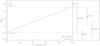 |
Fig. 1 a) Relation between fodd and the r-process contribution calculated from Arlandini et al. (1999). Coefficients are given where fodd = a × r-process (%) + b. b) LAP02: the Lambert & Allende Prieto (2002) result for fodd. M95: the Magain (1995) result for fodd. CAN1D: the Collet et al. (2009) 1D LTE result for fodd. CAN3D: the Collet et al. (2009) 3D hydrodynamical result for fodd. |
Magain (1995) attempted to verify Truran’s proposal by measuring the odd fraction in HD 140283, a well studied metal-poor subgiant at [Fe/H ] = −2.5 (Aoki et al. 2004), but found instead that theory and observations were not comparable. He used high-resolution (R ≡ λ/Δλ = 100000) high signal-to-noise (S / N ≈ 400) data. Magain reported the fractional odd isotope ratio, fodd, of Ba to be 0.08 ± 0.06, implying that Ba production in HD 140283 is predominantly due to the s-process (see Fig. 1b) despite [Fe/H] and [Ba/Fe] being very low, [Ba/Fe ] = −0.8 (Spite & Spite 1978). The code used to resolve the macroturbulence and analyse the Ba ii 4554 Å line solves the equations of hydrostatic equilibrium under the assumption that the stellar atmosphere has a plane-parallel geometry (1D) and local thermodynamic equilibrium (LTE). In contrast some more recent analyses, which we describe below, compute hydrodynamical 3D model atmospheres (3D) where the radiative transfer along multiple lines of sight is assessed.
The star was later reanalysed by Lambert & Allende Prieto (2002), again assuming 1D LTE. They obtained a very high-resolution (R ≡ λ / Δλ = 200000) high signal-to-noise (S / N ≈ 550) spectrum about the Ba ii 4554 Å line. They found a value for fodd = 0.30 ± 0.21 and concluded that, contrary to Magain’s result, the star is r-process dominated. A value for fodd = 0.30 ± 0.21 would imply an r-process contribution of 54% ± 60%. We note, however, that the error in their measurement of fodd means that their result covers the full range of possibilities from a pure s-process mix (fodd,s = 0.11) to a pure r-process mix (fodd,r = 0.46); see Fig. 1. This means that although they state that their result indicates that HD 140283 is r-process dominated, the range of fodd is too broad to be conclusive. We consider that an r-process contribution of 54% does not substantially imply that the star’s neutron-capture elements are dominated by those synthesised via the r-process.
Against this background, we sought to improve the determination of the s-process contribution to Ba in this star to help us understand the apparent conflicts.
While we conducted our study, Collet et al. (2009)
reanalysed the Lambert & Allende Prieto (2002)
spectrum in 1D LTE and, more significantly, also conducted a new 3D hydrodynamical analysis
of the Ba isotopic fraction of HD 140283. In 1D LTE they found that
fodd = 0.33 ± 0.13, meaning that 64% ± 36% of the Ba isotopes
in HD 140283 are synthesized via the r-process. The central value (0.33) is
little changed from that obtained by Lambert &
Allende Prieto (2002) (0.30), which is not entirely suprising since they used the
same spectrum, but Collet et al. (2009) quote smaller
error bars. This is because Lambert & Allende Prieto
(2002) adopted the standard deviation of macroturbulent broadening estimates as the
main underlying measurement error. Collet et al.
(2009) use the standard error  (where N is the number of Fe lines used) as
a measurement of error. The latter is a more reasonable estimate of the error as it is a
measure of the uncertainty in the mean estimate of the broadening. Their analysis of the
line using 3D hydrodynamics gives a value for fodd = 0.15 ± 0.12
meaning only 11% ± 34% of the isotopes are synthesized via the r-process.
This value is in good agreement with the solar Ba isotopic mix
(fodd,ss = 0.16 implying that only 14% of
isotopes formed via the r-process Arlandini
et al. 1999) but is once more at odds with the high r-process
fraction expected under Truran’s hypothesis.
(where N is the number of Fe lines used) as
a measurement of error. The latter is a more reasonable estimate of the error as it is a
measure of the uncertainty in the mean estimate of the broadening. Their analysis of the
line using 3D hydrodynamics gives a value for fodd = 0.15 ± 0.12
meaning only 11% ± 34% of the isotopes are synthesized via the r-process.
This value is in good agreement with the solar Ba isotopic mix
(fodd,ss = 0.16 implying that only 14% of
isotopes formed via the r-process Arlandini
et al. 1999) but is once more at odds with the high r-process
fraction expected under Truran’s hypothesis.
We have obtained a high resolution (R ≡ λ/Δλ = 95000) very high signal-to-noise (S/N = 870 − 1110) spectrum of HD 140283. During the course of this paper we discuss how we have constrained the macroturbulence by fitting synthetic spectra to Fe lines. In a detailed error analysis we show how we have improved constraining the macroturbulence, which was a major source of error that dominated previous studies that analyse the Ba ii 4554 Å line in 1D LTE. The improvement is partly due to the higher quality spectrum we have used in this investigation. We also explore the impact of using radial-tangential macroturbulence, ζRT, and rotational broadening, vsini (used by Collet et al. 2009) to help constrain macroscopic broadening. We then move on to discuss the method used to re-evaluate the r- vs. s-process mix by analysing the Ba ii 4554 Å line and, for the first time in this context, the Ba ii 4934 Å line in 1D LTE. Furthermore we discuss the difficulties in analysing the Ba ii 4934 Å line due to close blends with other lines. Also because of the exceptional quality of the data, we have been able to revise downward the Eu abundance limit for the star.
2. Observational data
Our stellar and ThAr calibration spectra were obtained over two nights during the commissioning of the High Dispersion Spectrograph (HDS) mounted on the Subaru Telescope. The stellar spectrum is the sum of 13 exposures totalling 82 min. This gives a S/N = 1110 per 12 mÅ wide pixel around the Ba ii 4554 Å line and a S/N = 870 per 12 mÅ wide pixel around the Ba ii 4934 Å line, as measured from the scatter in the continuum of the reduced spectrum. The typical resolution as measured from ThAr lines is R ≡ λ/Δλ = 95000. The spectrum was reduced using a ThAr spectrum to wavelength calibrate the stellar spectrum, with typical rms errors of 1.5 mÅ (Aoki et al. 2004). We utilise the 4554 Å and 4934 Å lines as both arise from the ground state where hyperfine structure is large. Although the 4934 Å line is weaker – we measure equivalent widths W4554 = 20.1mÅ and W4934 = 13.6 mÅ – the hfs of the 4934 Å line is greater, which means both lines can be useful diagnostics. We do not attempt to analyse higher excitation lines of Ba which are weaker and have much smaller hfs.
3. Spectral profiles
To analyse the two Ba ii line profiles in our spectrum we compared our observed profile to synthetic profiles produced by the 1D LTE code ATLAS (Cottrell & Norris 1978). We describe below how Fe i and Fe ii lines are used to constrain macroturbulence, and then proceed to analyse the Ba ii lines. A 1D KURUCZ06 model atmosphere (http://kurucz.harvard.edu/grids.html) was used with parameters for the star Teff = 5750 K, [Fe/H] = −2.5 and microturbulence, ξ = 1.4 kms-1 (Aoki et al. 2004) and log g = 3.7 [cgs] (Collet et al. 2009).
3.1. Instrumental profile
Two ThAr hollow-cathode-lamp spectra over the intervals 4102 − 5343 Å and 5514 − 6868 Å,
taken during the observing run with the same instrumentation and set-up as the stellar
exposures used in this study, were used to calculate the instrumental broadening. Using
IRAF, the full-width at half-maximum (FWHM) and equivalent widths of 993 emission lines
were measured. It was found that at a wavelength of 4554 Å the ThAr line FWHM in velocity
space (νinst) was 3.31 kms-1, and at 4934 Å was
3.25 kms-1. The error in these measurements is taken as the standard error
of the mean of the individual measurements, , which is 0.01 kms-1, where σ
is the standard deviation of the individual measurements, which is
0.22 kms-1. We assume here that the ThAr lines are unresolved and hence that
the measured ThAr line width represents the instrumental broadening. The instrumental
broadening could be slightly less than that stated, but the difference is immaterial
since, in Sect. 3.2, we measure the combined
instrumental and macroturbulent broadening without needing to distinguish between the two
contributions precisely. Aoki et al. (2004) showed
that the instrumental profile is well approximated by a Gaussian.
3.2. Macroturbulence
Lambert & Allende Prieto (2002) established that one of the major limiting factors in their analysis was the accuracy with which macroturbulence could be measured. They found that δfodd / δFWHM = − 0.51 (km s-1)-1, and hence for σFWHM = 0.33 kms-1 they achieved an accuracy in macroturbulence corresponding to σfodd ~ 0.17, dominating their total error of 0.21. It was clear that we would have to improve on this significantly to make progress.
We began to constrain macroturbulence by measuring the equivalent widths and the FWHM (in velocity space), νobs, of 257 apparently unblended Fe i and Fe ii lines by fitting Gaussian profiles in IRAF. We used this information to produce Fig. 2. As Δλ/λ remains constant with wavelength in an echelle spectrum (where Δλ is the width of the pixel in wavelength units) it is possible to use Fig. 2 as a check of the quality of measurements.
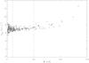 |
Fig. 2 FWHM versus equivalent width for the 257 Fe i and Fe ii measured for HD 140283. 93 lines fall into the range of 10 ≤ W (mÅ) ≤ 50; the mean value for νobs in this range is 6.9 kms-1. |
From Fig. 2 we can see that weaker lines, W ≤ 50mÅ, almost form a plateau. Here, νobs remains constant even as the Doppler core deepens in lines on the linear part of the curve of growth, where the Doppler broadening components are dominant. At W > 50 mÅ, pressure broadening become significant as the core of the line saturates, so the wings begin to broaden. Where W < 10 mÅ, the uncertainty produced by the finite signal-to-noise makes it difficult to measure the lines accurately, which is shown by the scatter in this region of Fig. 2.
Of the 257 Fe lines measured, 93 fell between 10 mÅ ≤ W ≤ 50 mÅ and were used to constrain macroturbulence (recall that W4554 = 20.1 mÅ and W4934 = 13.6 mÅ). The average value for the observed velocity FWHM, νobs, in this range is 6.9 kms-1. The full list of measurements can be found in Table A.1.
3.2.1. Gaussian macroturbulence
We convolve the synthetic flux spectrum of the star with a Gaussian of FWHM νconv which represents the convolution of the Gaussian instrumental profile with a Gaussian macroturbulent profile. For now we assume that the star has no significant rotation; we shall return to this point in Sect. 3.2.2. Current estimates of rotation of HD 140283 are vsini = 5.0 ± 2.0 kms-1 (de Medeiros et al. 2006). We create a grid of 385 convolved synthetic spectra for 11 values of macroturbulence 4.9 kms-1 ≤ νconv ≤ 6.9 kms-1 in steps Δνconv = 0.1 kms-1 and 35 values for A(Fe)3, with steps . Each synthetic spectrum covered the wavelength range 4100 − 6900 Å in intervals of Δλ = 0.01 Å.
To determine the best fit for νconv we compare our
synthetic model grid to the observed spectrum employing a χ2
test,  , where Oi is
the observed continuum-normalised profile,
Mi is the model profile of the line
produced using ATLAS and
, where Oi is
the observed continuum-normalised profile,
Mi is the model profile of the line
produced using ATLAS and  is the standard deviation of the observed points that
define the continuum, i.e.
σ = (S / N)-1. All 93
Fe i and Fe ii lines were individually fitted using a
χ2 code (García Pérez
et al. 2009). This code allows small wavelength shifts, Δλ,
which we discuss below and local renormalisation of the continuum of the observed
profile for every line. It finds values for Δλ, A(Fe)
and macroturbulence that minimize χ2 for each Fe line
analysed over a window 0.6 Å wide and with continuum windows typically 0.5 Å to 1.0 Å on
each side of this, depending on neighbouring spectral features. Values of
νconv found by the χ2 code for
the 93 lines covering the wavelength range 4118 − 6253 Å are shown in Fig. 3. The full table of results from the
χ2 code is found in Table A.1.
is the standard deviation of the observed points that
define the continuum, i.e.
σ = (S / N)-1. All 93
Fe i and Fe ii lines were individually fitted using a
χ2 code (García Pérez
et al. 2009). This code allows small wavelength shifts, Δλ,
which we discuss below and local renormalisation of the continuum of the observed
profile for every line. It finds values for Δλ, A(Fe)
and macroturbulence that minimize χ2 for each Fe line
analysed over a window 0.6 Å wide and with continuum windows typically 0.5 Å to 1.0 Å on
each side of this, depending on neighbouring spectral features. Values of
νconv found by the χ2 code for
the 93 lines covering the wavelength range 4118 − 6253 Å are shown in Fig. 3. The full table of results from the
χ2 code is found in Table A.1.
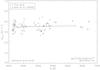 |
Fig. 3 Values of νconv that satisfy the minimum value for
χ2 for the 93 lines (plus symbols).
The standard error represents the scatter from the mean of each line
( |
We use an ordinary least squares (OLS) fit to determine
νconv at the wavelengths 4554 Å and 4934 Å. The OLS has
the equation
νconv = aλ + b, where
a and b are coefficients of the OLS. We find that
νconv = 5.75 kms-1 and
νconv = 5.76 kms-1 at the Ba ii
4554 Å and 4934 Å lines respectively. The error in these values, represented by the
standard error, is 0.02 kms-1. As the uncertainty in these values is
greater than the difference between them, we adopted one value for
νconv for both Ba ii lines,
νconv = 5.75 ± 0.02 kms-1. Subtracting the
instrumental FWHM at 4554 Å we find the macroturbulence, νΓ,
to be  . This value agrees well with that found by Aoki et al. (2004). The error in
νΓ is given by
. This value agrees well with that found by Aoki et al. (2004). The error in
νΓ is given by  , which is equal to ± 0.02 kms-1.
In using the Fe lines to determine the macroturbulence appropriate to Ba, it is important that we measure lines forming over a similar range of depths in the photosphere. This was achieved in the first instance by restricting the equivalent width range of the Fe lines to span the two Ba lines (see Fig. 2). In addition, we have regressed the νconv measurements against equivalent width, W, and against excitation energy, χ, and find no statistically significant trend of νconv with W, and a weak (2.5σ) trend with χ. This suggests that using a stricter restriction on the Fe line list would not materially alter the macroturbulent velocity. In the most extreme case, the value for χ = 0 eV would imply νconv = 5.62 ± 0.05 kms-1, which (as we show below) would increase fodd by 0.09.
The χ2 code also determined that , where the error is taken as the standard error. Taking the solar Fe abundance to be A(Fe)⊙ = 7.50 ± 0.05 from Grevesse & Sauval (1998), we calculate the metallicity, [Fe/H] = −2.59 ± 0.05, where the error in [Fe/H] is the propagation of the statistical error in and but so far excludes the systematic errors associated with the imperfect choice of atmospheric parameters. That error, based on calculations we provide in Sect. 5, is around 0.07 dex, giving a total error of 0.09 dex. This is in good agreement with metallicity we adopted from Aoki et al. (2004). We note that there is an updated list of solar abundances given in Grevesse et al. (2007) calculated using 3D hydrodynamics, however we decided to use the 1D LTE results given in Grevesse & Sauval (1998) as we are working in 1D LTE.
We found that the mean wavelength shift, Δλ, was −12.0 mÅ with a standard deviation σΔλ = 3.8 mÅ. There are several reasons why we would expect to find a wavelength shift between the observed and synthetic profiles. The most likely is an error in the approximate radial velocity correction of the star, but line-to-line differences require further comment. There could be inaccuracies in the assumed wavelengths in the Fe line list, however the Fe line list was produced using the most up to date data available through the IRON PROJECT and Nave et al. (1994), where wavelengths are quoted to 1 mÅ, and are believed to be accurate to < 1 mÅ. The rms error in the wavelength calibration was reported as only 1.5 mÅ (Aoki et al. 2004), so the line-to-line scatter σΔλ exceeds that error. The excess could be due to the inability of 1D hydrostatic model atmospheres to model turbulent motions in a star’s hydrodynamic atmosphere. Indeed, the residuals shifts were found to depend, at least partially, on the excitation potential, χ, and the equivalent width, W, suggesting an astrophysical cause.
3.2.2. Non-Gaussian symmetric broadening
So far we have adopted a Gaussian macroturbulent broadening mechanism. We looked at two other macro-scale broadening mechanisms, radial-tangential macroturbulence (ζrt) and rotation (vsini) (Gray 2008, Chap. 18). Each broadening run was given the same atmospheric parameter set; Teff = 5750 K, log g = 3.7, [ Fe / H ] = − 2.5, ξ = 1.4 kms-1. Table 1 shows the results from fitting the 93 Fe lines using the three broadening types, along with Gaussian instrumental broadening (νinst = 3.31 kms-1). The third column indicates how many of the 93 lines were best fit by that broadening mechanism, as judged by the minimum χ2 value for the three methods.
Comparison of all three broadening types.
Only three of the 93 Fe lines were fit best by rotational broadening, and hence we concluded that using only rotational velocities to broaden the lines would be unsound. The derived value provides a firm upper limit on rotation, vsini ≤ 3.9 kms-1, in the case with no macroturbulent broadening. The fact that most lines are fit better by a macroturbulent profile emphasises that we have not detected true rotation of the star at this 3.9 kms-1 level.
The radial-tangential broadening function within the 1D LTE framework, provides a better fit than Gaussian macroturbulence to almost two thirds of the Fe lines. We present Ba results for both macroturbulent prescriptions in Sect. 4.4, but unless specified, our analysis is conducted using Gaussian fitting.
4. The Ba II resonance lines and the barium isotopic ratio
4.1. Ba II line structure
There are five principal, stable Ba isotopes that are formed via the two neutron-capture processes. The r- and s-process produce different mixes of odd and even isotopes. The r-process does not contribute to two even isotopes, 134,136Ba, which are pure s-process isotopes. The two odd isotopes, 135,137Ba, and even isotope 138Ba are formed from both the s- and r-process. The odd isotopes broaden the line and make it asymmetric, whereas the even isotopes contribute to the centre of the Ba ii line and make the core deeper.
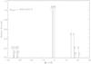 |
Fig. 4 The splitting patterns of the Ba ii 4554 Å line relative to 138Ba. The relative strengths of each isotope are normalised to 1 (Table 2, Col. (3)). |
The isotopic and hfs information for both Ba lines.
4.2. χ2 test
The observed continuum was renormalised over a window of 1 Å either side of each of the two Ba lines. A new grid comprising 231 synthetic spectra around each of the two Ba ii resonance lines was produced in ATLAS. Values for νconv and A(Fe), constrained in the last section, were fixed. There were three free parameters in the new grid: A(Ba), Δλ and the r- and s-process contributions. The χ2 code allowed small changes in these parameters exactly like the code described in Sect. 3.2.1. We used 21 values for A(Ba), − 1.40 ≤ A(Ba) ≤ − 1.20, where . Each synthetic spectrum covered the range 4550 − 4560 Å (around 4554 Å), 4930 − 4940 Å (around 4934 Å) and was computed every 0.01 Å. The windows in which both Ba lines were analysed was ± 0.25 Å from their centroid.
4.3. The iron blends at 4934 Å
It has been documented that the Ba ii 4934 Å line has a known blend with a weak Fe i line (Cowley & Frey 1989). We use the information for two Fe lines which are found in Nave et al. (1994, their Table 2). The relevant data can be found in our Table 3.
Spectroscopic information on the two weak Fe lines that are blended with the Ba ii 4934 Å line as reported by Nave et al. (1994).
When these wavelengths are compared with the wavelengths for the Ba 4934 Å line given in Table 2 it is clear that the two Fe lines would influence the r-process fraction found by analysis of the line. This is shown in Fig. 5 for pure s- and r-process isotope ratios. The analysis of the 4934 Å line is very sensitive to the characteristics of the Fe lines, as we show in Sect. 5.2. We include these Fe lines in our Ba 4934 Å line analysis.
4.4. The r-process contribution
The Ba abundances of the two lines are found to be and . We take the implied Ba abundance as an average of the two, . Using the solar abundances calculated in Grevesse & Sauval (1998) we find that for HD 140283, [Ba/H] = −3.46 ± 0.11, and hence [Ba/Fe] = −0.87 ± 0.14. Errors stated here are calculated in Sect. 5. Results from other papers are given in Table 4. It is shown that our result for [Ba/Fe] is in good agreement with previous results.
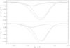 |
Fig. 5 Synthetic spectra showing the effect of the Fe i blends on the 4934 Å Ba ii line. The top plot shows the r-process-only isotope fraction and the bottom shows the s-process-only isotope fraction. Solid line: the underlying Fe i blends. Dashed line: the uncontaminated Ba ii line. Dash-dot line: the overall line profile. |
From the χ2 analysis we find the best statistical fit for the 4554 Å line is fodd = 0.01 ± 0.06. The best statistical fit for the 4934 Å line indicates a value of fodd = 0.11 ± 0.19 (meaning an r-process contribution of 0% ± 54%). The 1σ errors stated here arise from uncertainties discussed in Sect. 5 and are larger for the 4934 Å line because of uncertainties associated with the underlying Fe blends. Our result is in good agreement with Magain (1995) who found that Ba ii 4554 Å yielded fodd = 0.08 ± 0.06, but seems to be at odds with values found by Lambert & Allende Prieto (2002) (fodd = 0.30 ± 0.21) and the 1D result found for the same spectrum by Collet et al. (2009) (fodd = 0.33 ± 0.13).
The reduced chi-squared values,  , for the 4554 Å line and the 4934 Å line are 6.6 and 2.0
respectively. The two best statistical fits for both lines and their residuals (observed –
synthetic profiles) are shown in Fig. 6. We also plot
the synthetic profiles for the Ba lines with an r-process contribution of
100%, best fit for both lines. It can be seen in the residual plots for both lines that
the pure r-process fits are very poor. In 4554 Å,
, for the 4554 Å line and the 4934 Å line are 6.6 and 2.0
respectively. The two best statistical fits for both lines and their residuals (observed –
synthetic profiles) are shown in Fig. 6. We also plot
the synthetic profiles for the Ba lines with an r-process contribution of
100%, best fit for both lines. It can be seen in the residual plots for both lines that
the pure r-process fits are very poor. In 4554 Å,
 changes faster with fodd than
for the 4934 Å line. This indicates that although the 4934 Å line is broader due to the
effects of hyperfine structure, the 4554 Å line is more sensitive to changes in
fodd. This could be both because the 4554 Å line is stronger
(W = 20.1 mÅ) than the 4934 Å line (W = 13.6 mÅ), and
because the latter has an Fe blend.
changes faster with fodd than
for the 4934 Å line. This indicates that although the 4934 Å line is broader due to the
effects of hyperfine structure, the 4554 Å line is more sensitive to changes in
fodd. This could be both because the 4554 Å line is stronger
(W = 20.1 mÅ) than the 4934 Å line (W = 13.6 mÅ), and
because the latter has an Fe blend.
Based on the calculations by Arlandini et al.
(1999), our 4554 Å result should not be achievable, and corresponds to an
r-process contribution of − 29% (i.e. the s-process
contribution is equal to 129%). We have also plotted in Fig. 7 the fit and residual for the nearest physically possible value for
fodd (0.11). This fit has  . We have also plotted the fit for
fodd = 0.01, which is quite similar.
. We have also plotted the fit for
fodd = 0.01, which is quite similar.
Results from previous studies of HD 140283.
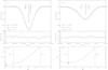 |
Fig. 6 Panel a) i): the best statistical fit synthetic profile (solid line) for the observed Ba ii 4554 Å line (diamonds) with the residual and χ2 plots below. For comparison, a pure r-process line and residual has been plotted (dash-dot line). The value for has been optimised to one that minimises χ2, values for and macroturbulence remain the same. Panel a) ii): the χ2 fit for the 4554 Å line, the cross shows where the minimum of the fit lies. Also plotted are the splitting patterns for barium relative to barium-138 (see Table 2). Panels b) i) and ii): show the same as a) i) and ii) for the 4934 Å line. |
When we adopted radial-tangential macroturbulence, it was determined that
fodd = − 0.02 ± 0.06 and − 0.03 ± 0.19 for the 4554 Å and
4934 Å lines respectively, with  and 2.8. Errors stated here are assumed to be the same as
those calculated using a Gaussian macroturbulence as only the broadening mechanism
differs; the errors in the two broadening techniques have the same value. The best fits
are shown in Fig. 8. So the radial-tangential fit for
the 4554 Å line is a statistically better fit than the Gaussian macroturbulent fit, as
seen by the residual plots (Figs. 6a, i and b, i vs.
Figs. 8a, b). Both broadening mechanisms, which
were analysed separately, yield similar values for Δλ,
fodd and [Ba/H]. Both indicate a strong
s-process signature for barium. Although these
fodd numbers are again beyond possible physical values, we
inform the reader that due to the finite confidence in the test (discussed further in Sect. 7), the unphysical values fodd ≃ 0.01 are
not greatly preferred over the physical value fodd = 0.11.
and 2.8. Errors stated here are assumed to be the same as
those calculated using a Gaussian macroturbulence as only the broadening mechanism
differs; the errors in the two broadening techniques have the same value. The best fits
are shown in Fig. 8. So the radial-tangential fit for
the 4554 Å line is a statistically better fit than the Gaussian macroturbulent fit, as
seen by the residual plots (Figs. 6a, i and b, i vs.
Figs. 8a, b). Both broadening mechanisms, which
were analysed separately, yield similar values for Δλ,
fodd and [Ba/H]. Both indicate a strong
s-process signature for barium. Although these
fodd numbers are again beyond possible physical values, we
inform the reader that due to the finite confidence in the test (discussed further in Sect. 7), the unphysical values fodd ≃ 0.01 are
not greatly preferred over the physical value fodd = 0.11.
We have given values for fodd for the two Ba lines and we have shown that the two lines are in agreement within the stated errors. We now discuss those uncertainties and what stellar parameters fodd is sensitive to.
5. Uncertainties and sensitivity tests
In this section we scrutinise the analysis procedures and statistical tests employed in this study to determine the likely statistical and systematic errors. These include errors associated with the atmospheric parameters used in constructing the synthetic spectra, the calculated macroturbulence and the errors associated with the iron lines used in conjunction with the Ba 4934 Å line.
Table 5 lists values found for [Ba/H] and fodd by varying the temperature and log g of the model atmosphere. There are two cases. In case 1 we recalculate [Fe/H] and macroturbulence for every value of Teff and log g, whereas in case 2 we fix the macroturbulence and [Fe/H] to values calculated for Teff = 5750 K and log g = 3.7. Perhaps the first thing to note from this table is that altering temperature by ± 250 K and log g by ± 0.3 does not drive fodd to an r-process dominated fraction. The errors quoted in this paper for HD 140283 are based on uncertainties in Teff and log g of ± 100 K and ± 0.1 respectively.
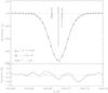 |
Fig. 7 Comparison between the nearest physical fit (solid line) where fodd = 0.11 and the best statistical fit (dash-dot line) where fodd = 0.01, for the 4554 Å line. Also plotted are the splitting patterns for barium relative to barium-138 (see Table 2). |
From Table 5 it is possible to calculate the error associated with [Fe/H], , and hence [Ba/H] & [Ba/Fe], by examining how it is affected by the stellar parameters. We use case 1 to calculate these uncertainties. It is shown in Table 5 that gravity as very little affect on [Fe/H]. Temperature has a much greater affect on [Fe/H], altering the ratio by ± 0.07 dex for every 100 K. Therefore we find a total uncertainty in [Fe/H] of ± 0.07. We find that . Therefore an error of 0.1 in log g implies an error . Similarly we find for temperature that . Taking the uncertainty in temperature to be ± 100 K we find that . Macroturbulence affects the shape of lines but not the equivalent width. As such we do not include the uncertainties associated with macroturbulence here. Also [Fe/H] has very little affect on [Ba/H] when compared to temperature and gravity effects so this is not included in our error analysis of [Ba/H]. The solar barium abundance is (Grevesse & Sauval 1998). When these uncertainties are added in quadrature we find that [ Ba / H ] = − 3.46 ± 0.11. Therefore we find that [ Ba / Fe ] = − 0.87 ± 0.14.
5.1. The 4554 Å line
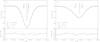 |
Fig. 8 Panel a): the best statistical fit for the 4554 Å line (diamonds) using a radial-tangential velocity profile (solid line). We have included a pure r-process, fodd = 0.46, synthetic profile for comparison (dash-dot line). Also plotted are the splitting patterns for barium relative to barium-138 (see Table 2). Panel b): same as panel a) but for the 4934 Å line. |
The sensitivity to [Fe/H], [Ba/H], νconv and fodd for different values of Teff and log g.
We have stated that potentially the most significant parameter that fodd is sensitive to is macroturbulence. The difference between Cols. 9 and 10 in Table 5 show how fodd is sensitive to macroturbulence. We find that on average, δfodd/δνconv ⋍ −0.7 (kms-1)-1 meaning that for σνconv = 0.02 kms-1, calculated in Sect. 3.2, σfodd ⋍ 0.01. That is, by using a large number of Fe lines to constrain νconv, we have minimized the impact of this error.
Realistically, when you vary one parameter you alter all other parameters to compensate for this change. Increasing temperature increases the derived macroturbulence, which on its own decreases fodd. For case 1 we see that an uncertainty in temperature of ± 100 K implies an uncertainty in macroturbulence of 0.01 kms-1 to 0.02 kms-1 with increasing gravity (see Table 5, Col. (3)). Using the relation we found between fodd and macroturbulence we see that σfodd = 0.02 to 0.06. In case 2 (where we only look at how fodd is affected by one stellar parameter) we find that for an error in temperature of ± 100 K, σfodd ≈ ± 0.004 to 0.01 depending on log g (Table 5 Col. (10), case 2).
The uncertainty in log g for HD 140283 is quite small, ≲ 0.1, due to its reliable Hipparcos parallax. As gravity affects line broadening, we find that log g influences the macroturbulence and fodd. Firstly we calculate the effect of log g on macroturbulence (case 1). We find δνconv / δlog g ⋍ 0.4 kms-1 depending on temperature. So for an uncertainty in log g = 0.1, σνconv ⋍ 0.04 kms-1. Using the sensitivity we calculated for macroturbulence suggests an uncertainty in fodd ⋍ 0.03. In comparison, the total case 1 sensitivity is δfodd / δlog g ≈ 0.2 implying σfodd = 0.02. We can see from Table 5 the separate effect that log g has on fodd when we fix macroturbulence (case 2). Here we find that δfodd / δlog g ⋍ − 0.17 meaning that an error in log g of 0.1 alters fodd directly by 0.02. The implication is that some of the change in case 1 is driven by the revision of the macroturbulence, and some is driven more directly but in a way that partially compensates.
When examining the effect of microturbulence on fodd one would expect to see two things. If we allow macroturbulence to compensate for the change in microturbulence (case 1) we would expect find that fodd is essentially unchanged. If we fix macroturbulence and alter microturbulence, fodd will change. Table 6 shows these two cases. As expected in case 1, the macroturbulence is driven up/down when the microturbulence is decreased/increased and fodd is unaffected. In case 2 we see the sensitivity in fodd as microturbulence is altered given by δfodd / δξ = − 0.5 (kms-1)-1. Therefore an uncertainty in microturbulence of 0.1 kms-1 implies an error in fodd = 0.05. It is case 1 that is relevant to our Ba analysis.
The sensitivity of fodd to ξ. Temperature and log g are fixed at 5750 K and 3.7 respectively.
In summary we can assign an uncertainty in fodd for the
4554 Å line  (case 1 – remember that νconv
compensates for any effect ξ has on fodd). In
case 2, where we look at the separate effects the stellar parameters have on
fodd, we find that for uncertainties in macroturbulence,
temperature, log g and microturbulence
(case 1 – remember that νconv
compensates for any effect ξ has on fodd). In
case 2, where we look at the separate effects the stellar parameters have on
fodd, we find that for uncertainties in macroturbulence,
temperature, log g and microturbulence  . Case 1 is probably more applicable, but we adopt the
larger error, case 2, as a precaution, i.e. ± 0.06. We now move on to errors and
uncertainties associated with the 4934 Å line.
. Case 1 is probably more applicable, but we adopt the
larger error, case 2, as a precaution, i.e. ± 0.06. We now move on to errors and
uncertainties associated with the 4934 Å line.
5.2. The 4934 Å line
In order to assign an uncertainty in fodd to the 4934 Å line we must also explore how uncertainties in the Fe blend (see Table 3) affect fodd.
We explored how the equivalent width of the Fe blend is affected by temperature and log g. As in Tables 5 and 6, we computed two cases where we allow macroturbulence and [Fe/H] to vary with varying temperature and log g (case 1) and where we have fixed macroturbulence and [Fe/H] (case 2) – in Table 5.
The net result of an increase in log g, decrease in macroturbulence, and increase in [Fe/H], is a small increase in synthesized WFe, but these effects are minimal compared to the effects that macroturbulence has on fodd. Consequently we see a similar behaviour in fodd (Table 5, Col. (11)) as that exhibited by the 4554 Å line (Col. (9)) (a roughly linear increase in fodd with log g with Δfodd,4934 comparable to Δfodd,4554).
In case 2 an increasing temperature decreases the equivalent widths of the Fe lines. Unlike case 1, macroturbulence and are not compensating for the increasing ionisation fraction meaning that Fe i level populations are decreasing. This decreases the strength of the Fe lines, decreasing their equivalent widths.
As log g is driven up in case 2, we find that the equivalent widths are decreasing, recall that is fixed in case 2. Overall, however, we see little or no change in fodd in Col. (12) in Table 5.
Values of fodd for the 4934 Å line found from altering the strength of the Fe lines.
We also investigate how the log gf values, which are not well known for the two Fe lines, affect fodd. The 4934 Å line is driven to a pure r-process fraction if the Fe blend is eliminated from the line list, so we would expect that fodd would be quite sensitive to log gf. Table 3 shows the parameters of the two lines. We analyse the case that the log gf values have an error ±0.15 as a heuristic estimate. Table 7 shows how fodd for the 4934 Å line is affected by this increase/decrease in Fe strength. We have tabulated the results for fodd for all values of temperature and log g we use in our sensitivity analysis. It can be seen for case 2 at a temperature of 5500 K and where the Fe blend strengths have been increased, that fodd becomes so small and so unphysical that our χ2 program cannot find a minimum solution. Similarly this is seen in case 1 at a temperature of 6000 K. It is clear from Table 7 that for 4934 Å, fodd is more sensitive to the uncertainty in the strengths of the Fe lines than the atmospheric parameters. We see in case 1 that as we alter the Fe log gf by ±0.15, fodd is altered by ∓0.18. This means that when added in quadrature to the error discussed in Sect. 5.1, we find that for case 1, fodd = 0.11 ± 0.18. For case 2, fodd = 0.11 ± 0.19. We take the error to be the average of the two, so fodd = 0.11 ± 0.19.
5.3. Overall result
Inverse-variance-weighting the results for 4554 Å (0.01) and 4934 Å (0.11) give an overall result fodd = 0.02 ± 0.06 when macroturbulence is modelled as a Gaussian. When a radial-tangential broadening mechanism is used we find that inverse-variance-weighting gives an overall result fodd = −0.02 ± 0.06.
So far the uncertainties discussed in the section have been limited to errors in Teff, log g, νconv and log gf. We have not yet quantified the impact of finite S / N and possible systematic errors associated with a 1D LTE analysis. We recall from Sect. 3.2.1 that systematic errors of order 0.09 may arise from using Fe lines to estimate, in 1D, the macroturbulent broadening of Ba. We discuss this further in Sect. 7. We shall now move on and discuss the europium abundance and the various implications of the Ba and Eu results.
6. Europium abundance limit
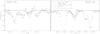 |
Fig. 9 Synthetic spectra for the Eu 4129 and 4205 Å lines for [ Eu / H ] = − 2.80 and for the abundances calculated in three other studies of this star (see text). It is clear that they over estimate the strength of both lines. While the 4205 Å line includes several blends particularly V ii 4205.09 Å, the 4129 Å has none. We show the V ii line separately in the right-hand panel (dot-line). |
Within our spectral range (4118 − 6253 Å) there are two Eu ii resonance lines, 4129.70 Å and 4205.05 Å. Honda et al. (2006) report that the latter has a known blend with a V i line. Gilroy et al. (1988), Magain (1989) and Gratton & Sneden (1994) report [Eu/H] to be −2.31, −2.49 and −2.41 respectively. However, these lines do not appear strongly in our spectrum. This becomes clear when studying Fig. 9, which presents the observed data and several synthetic spectra. The Eu line lists were constructed using hyperfine splitting information from Krebs & Winkler (1960) and Becker et al. (1993). We acknowledge that more recent hyperfine splitting information is available from Lawler et al. (2001), which is in good agreement with Krebs & Winkler (1960) and Becker et al. (1993) but we do not use that data here. An isotopic ratio of 0.5:0.5 for Eu 151:153 was chosen for the r- and s-processes (the solar system isotopic ratio of Eu 151:153 is 0.48:0.52 Arlandini et al. 1999), and gf values from Biemont et al. (1982) and Karner et al. (1982) were used. The synthetic spectra were produced using KURUCZ06 model atmospheres in conjunction with the 1D LTE code ATLAS. The macroturbulence and [Fe/H] was set at values calculated in Sect. 3.2.1.
The Eu 4205 Å synthesis includes several blends which we have adopted from the Kurucz theoretical database (http://www.cfa.harvard.edu/amp/ampdata/kurucz23/sekur.html). The dominant blend is a V ii line at λ = 4205.09 Å, which has a gf value of 0.089 and χ = 2.04 eV. The abundance of V was taken as the solar abundance scaled to the metallicity. We found no blends associated with the 4129 Å line. As these line blends are theoretical, we make no claim that the abundances we deduce from the Eu analysis are as accurate as the analysis conducted on the Ba lines. We interpret the absorption feature at 4205.1 Å as due to V ii, not Eu, as it is much narrower than the synthesised, hfs-broadened Eu line. Moreover if it were Eu, not V, it would require an abundance inconsistent with the weakness of the Eu 4129 Å line. We find that a [Eu/H] abundance of − 2.80 seems to be a generous upper limit on the Eu abundance, rather than a genuine detection and lower than the cited detections. Therefore we assign a lower limit [ Ba / Eu ] > − 0.66. This marginally excludes an r-process ratio, whether we assume an r-process limit set in Burris et al. (2000) ( − 0.81, which were calculated using the Anders & Grevesse (1989) isotopic abundances) or Arlandini et al. (1999) ( − 0.69). A pure s-process ratio ( + 1.45, Burris et al. 2000 or + 1.13, Arlandini et al. 1999) or a mixed s- and r-process regime, is compatible with the data. However, our [Ba/Eu] limit does agree well with observations found in François et al. (2007) for stars of similar metallicity to HD 140283.
We shall now move on and discuss the various implications of the results found in this paper and look at possible solutions to reduce systematic errors associated with a 1D LTE analysis.
7. Discussion
We have found that fodd = 0.02 ± 0.06, and hence the r-process fraction implies a purely s-process signature of Ba in HD 140283. The [Ba/Eu] ratio, > −0.66, is also marginally inconsistent with a pure r-process regime. The isotope result does not entirely contradict previous work by Lambert & Allende Prieto (2002) and Collet et al. (2009) since, due to the size of their 1σ errors, an s- or r-process isotopic mixture was feasible (see Fig. 1). Although we find that fodd for the 4554 Å line is unphysical (at the 1.8σ level) based on Arlandini et al. (1999), we must consider the possibility that the adopted s- and r-process isotope contributions may not be accurate, as they are based on our simplified understanding of nucleosynthesis, which could be flawed. For example, the Arlandini et al. (1999) calculations give a solar-system r-process isotopic ratio, and we cannot be certain that this applies in the Galactic halo. However, metal-poor stars with r-process enhancements do not least have similar neutron-capture abundance patterns to the sun, e.g. CS 22892-052 (Sneden et al. 1996).
We also question whether the S / N ratio is high enough
to measure these fractions accurately, and whether a 1D LTE analysis is an adequate tool in
investigating isotopic ratios at these high levels of
S / N, by looking at the confidence limits of the
χ2 minima, which we now discuss. The fact that our best
fitting spectra have values significantly greater than 1
( and 2.0 for the 4554 Å and 4934 Å line respectively)
indicates that the χ2 denominator
(σi) is not a good description of the
deviation of the model spectrum from the data. We interpret the high
values to indicate that systematic errors are present which
exceed the random fluctuations in the signal. This influence is confirmed by inspection of
Figs. 6 − 8,
where it can be seen that the residuals do not oscillate randomly from one pixel to the next
but rather seem to meander over a cycle of a few pixels. In short, this tells us that the
failure of the model profile to match to the data exceeds the error due to noise (mostly
photon noise) in the spectrum, and hence σi as
judged from the S / N underestimates the true residual.
From Fig. 6 it can be seen that the best fit under-fits
the core of the lines in order to fit the wings of the lines better. The
r-process contributes more to the wings of the line, see Fig. 4 and Table 2. It is
interesting to note that we under-fit the red wing of the 4554 Å line between 4554.11 Å and
4554.17 Å (see Figs. 6 and 7). Lambert & Allende Prieto
(2002) and Collet et al. (2009) in 1D, see
the same residual feature at this wavelength interval. When they reanalysed the line in 3D,
Collet et al. (2009) appeared to remove the feature
in the wing. This would suggest that it is a result of convection in a 3D atmosphere rather
than a feature induced by inaccuracies when calculating the isotopic shifts. We suspect that
the error arises due to the assumptions used in 1D LTE codes that are unable to correctly
model physical conditions in a 3D atmosphere.
and 2.0 for the 4554 Å and 4934 Å line respectively)
indicates that the χ2 denominator
(σi) is not a good description of the
deviation of the model spectrum from the data. We interpret the high
values to indicate that systematic errors are present which
exceed the random fluctuations in the signal. This influence is confirmed by inspection of
Figs. 6 − 8,
where it can be seen that the residuals do not oscillate randomly from one pixel to the next
but rather seem to meander over a cycle of a few pixels. In short, this tells us that the
failure of the model profile to match to the data exceeds the error due to noise (mostly
photon noise) in the spectrum, and hence σi as
judged from the S / N underestimates the true residual.
From Fig. 6 it can be seen that the best fit under-fits
the core of the lines in order to fit the wings of the lines better. The
r-process contributes more to the wings of the line, see Fig. 4 and Table 2. It is
interesting to note that we under-fit the red wing of the 4554 Å line between 4554.11 Å and
4554.17 Å (see Figs. 6 and 7). Lambert & Allende Prieto
(2002) and Collet et al. (2009) in 1D, see
the same residual feature at this wavelength interval. When they reanalysed the line in 3D,
Collet et al. (2009) appeared to remove the feature
in the wing. This would suggest that it is a result of convection in a 3D atmosphere rather
than a feature induced by inaccuracies when calculating the isotopic shifts. We suspect that
the error arises due to the assumptions used in 1D LTE codes that are unable to correctly
model physical conditions in a 3D atmosphere.
To explore this further, we have searched for evidence of asymmetries in the Fe-line data. We have produced two Fe-line plots by co-adding the residuals from all 93 lines to find an average residual, shown in Fig. 10 (top panel). The lower panel shows the average residual for the 82 Fe lines found to have no additional features or close non-Fe lines within the window over which the χ2 analysis is calculated (0.6 Å). Lines marked with an asterisk in Table A.1 denote the 11 Fe lines that were rejected. For one plot (dash-dot curve) the average residuals (obs-syn) are based on synthetic spectra calculated using the average wavelength shift (−12.04 mÅ) and average macroturbulence (5.75 kms-1) for all Fe-lines. The average residual is very asymmetric, in that the blue wings are better fit than the red wings. The large residuals in the red wings, around 60 − 170 mÅ from the line centre, are clearly not due to errors in the central wavelengths of the Fe lines, which are known to better than 1 mÅ (Sect. 3.2.1).
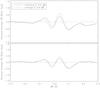 |
Fig. 10 Average residuals for fits to 93 Fe lines, for two cases. It is quite clear that assuming a constant wavelength shift and macroturbulence is adequate when working in 1D LTE but assuming 1D LTE when dealing with high quality data is not. Top panel: the reduced-noise residual plot for all 93 lines. Bottom panel: the reduced-noise residual plot for 82 lines without other close absorption features. Lines not included in lower panel are noted with an asterisk in Table A.1. |
We also computed a new set of synthetic spectra using the optimised νconv and Δλ values belonging to each Fe line as found from the χ2 analysis (see Table A.1), and recalculated the residuals (obs-syn) for these. These new residuals were coadded and averaged, and plotted in Fig. 10 (solid curve). These slightly reduce the overall amplitude of the residuals, as expected since we are optimising the fit to each Fe line. However, even after allowing each one to be optimised, the residuals are still quite asymmetric, with the red wings standing out as having larger residuals than the blue wings. From Fig. 10 we can see that a similar red feature to the one we see in Fig. 6 for Ba is present in both Fe residual plots, and appears at the same distance from the centroid of the Fe lines as the residuals for the Ba 4554 Å line (~100 mÅ). The feature remains whether we optimise νconv and Δλ or not. We suspect this feature may be the result of convection in the observed, dynamic atmosphere, similar to the feature seen in the Ba spectrum, that underlying assumptions in 1D LTE do not compensate for.
Collet et al. (2009) conduct a 3D analysis of HD 140283. Our measurements of the residuals for the Fe lines provide a future test of whether 3D modelling produces similar residuals. We hope to explore this at a later date. As the 3D process calculates the velocity field ab initio, there is no concept of micro- or macroturbulence in that framework. Consequently, Collet et al. (2009) ascribe any excess broadening to stellar rotation, and for this they infer vsini = 2.5 kms-1. We note that the upper limit on vsini which we infer for zero macroturbulence is 3.9 kms-1. Their value is compatible with our limit. We note that Collet et al. (2009) find a lower r-process fraction for HD 140283 using a 3D analysis than they find for 1D. If our findings are similar, then this will further accentuate the difference between the analysis of HD 140283 and the expectations based on Truran’s hypothesis.
One possible alternative explanation of the asymmetries is that we are seeing the combined spectra of more than one star, offset in velocity. It may be difficult to generate the observed levels of asymmetries for a realistic second star, and we have not attempted to do so, but note this possibility nonetheless. We also note that the radial velocity of HD 140283 has been steady to ± 0.35 kms-1 over long periods of time (Lucatello et al. 2005), decreasing the likelihood that it is a binary.
Finally we shall move on to discuss the conclusions we have drawn from our analysis of the isotopic ratio of Ba in HD 140283.
8. Conclusions
We have used very high quality data (S/N = 870 − 1110, R ≡ λ/Δλ = 95000) to analyse the Ba isotopic fraction and the Eu abundance limit in the metal-poor subgiant HD 140283. We obtain [Fe/H] = −2.59 ± 0.09, [Ba/Fe] = −0.87 ± 0.14, and [Eu/H] < −2.80. Using a 1D LTE analysis, we find fodd = 0.02 ± 0.06, corresponding to a Ba isotopic fraction which indicates a 100% contribution by the s-process. This result contradicts the theory put forward by Truran (1981). The result published by Lambert & Allende Prieto (2002) has error bars which are too broad to allow one to state conclusively that HD 140283 is r-process dominated. We have set a new lower limit to the [Ba/Eu] ratio, [Ba/Eu] > −0.66. This lower limit marginally rules out a pure r-process ratio in HD 140283, consistent with the isotopic fraction for barium. A new high resolution spectrum with a greater S/N around the 4129 Å line is needed to constrain a genuine abundance for Eu.
We have also carried out a careful examination of the 4934 Å line, which is more sensitive to the effects of hyperfine-splitting. We found that, due to the lack of laboratory gf data surrounding the Fe blend affecting the wings of this line, it is less effective as a tool to analyse the isotopic mixture than Ba 4554 Å.
By examining the spectral residuals for 93 Fe lines and for Ba 4554, 4934 Å, we find strong line asymmetries in the red wing. These may show the shortcomings of using a 1D LTE analysis to explore isotope ratios; using a more sophisticated 3D analysis may be warranted. We are looking to take this work further in the future and analyse HD 140283 using a 3D code. We note that Collet et al. (2009) find a lower r-process fraction for HD 140283 using a 3D analysis than they find for 1D. If our findings are similar, then this will further accentuate the difference between the analysis of HD 140283 and the expectations based on Truran’s hypothesis.
We set a new limit on the rotation of HD 140283: vsini < 3.9 kms-1.
Online material
Appendix A
The list of iron lines used to constrain νconv including measured W and νobs.
[X/Y![Mathematical equation: $]={\rm log}_{10}\big({\frac{N(X)}{N(Y)}}\big)_{*} - {\rm log}_{10}\big({\frac{N({\rm X})}{N({\rm Y})}}\big)_{\odot}\cdot$](/articles/aa/full_html/2010/15/aa14970-10/aa14970-10-eq329.png)
fodd ≡ [ N(135Ba) + N(137Ba) ] / N(Ba).
 .
.
Acknowledgments
The authors would like to acknowledge Satoshi Kawanomoto for reducing the stellar spectrum used in this work. A.J.G. and S.G.R. would like to thank Gillian Nave and Juliet Pickering for kindly investigating Fe spectra to constrain spectroscopic information about a known Fe blend in the Ba 4934 Å line which was crucial for the present investigation. S.G.R. wishes to acknowledge Ph.D. Thesis work by Blake (2004) on a spectrum of HD 140283 which, while not having the benefit of a large number of Fe lines for the determination of macroturbulence, nevertheless gave a value fodd = 0.08 ± 0.11.
References
- Anders, E., & Grevesse, N. 1989, Geochim. Cosmochim. Acta, 53, 197 [Google Scholar]
- Aoki, W., Inoue, S., Kawanomoto, S., et al. 2004, A&A, 428, 579 [NASA ADS] [CrossRef] [EDP Sciences] [Google Scholar]
- Argast, D., Samland, M., Thielemann, F.-K., & Qian, Y.-Z. 2004, A&A, 416, 997 [NASA ADS] [CrossRef] [EDP Sciences] [Google Scholar]
- Arlandini, C., Käppeler, F., Wisshak, K., et al. 1999, ApJ, 525, 886 [NASA ADS] [CrossRef] [Google Scholar]
- Becker, O., Enders, K., Werth, G., & Dembczynski, J. 1993, Phys. Rev. A, 48, 3546 [NASA ADS] [CrossRef] [PubMed] [Google Scholar]
- Biemont, E., Karner, C., Meyer, G., Traeger, F., & Zu Putlitz, G. 1982, A&A, 107, 166 [NASA ADS] [Google Scholar]
- Blake, L. A. J. 2004, Ph.D. Thesis, Open University (United Kingdom) [Google Scholar]
- Burbidge, E. M., Burbidge, G. R., Fowler, W. A., & Hoyle, F. 1957, Rev. Mod. Phys., 29, 547 [NASA ADS] [CrossRef] [Google Scholar]
- Burris, D. L., Pilachowski, C. A., Armandroff, T. E., et al. 2000, ApJ, 544, 302 [NASA ADS] [CrossRef] [Google Scholar]
- Busso, M., Gallino, R., Lambert, D. L., Travaglio, C., & Smith, V. V. 2001, ApJ, 557, 802 [NASA ADS] [CrossRef] [Google Scholar]
- Clayton, D. D., & Rassbach, M. E. 1967, ApJ, 148, 69 [NASA ADS] [CrossRef] [Google Scholar]
- Collet, R., Asplund, M., & Nissen, P. E. 2009, PASA, 26, 330 [NASA ADS] [CrossRef] [Google Scholar]
- Cottrell, P. L., & Norris, J. 1978, ApJ, 221, 893 [NASA ADS] [CrossRef] [Google Scholar]
- Cowley, C. R., & Frey, M. 1989, ApJ, 346, 1030 [NASA ADS] [CrossRef] [Google Scholar]
- de Medeiros, J. R., Silva, J. R. P., Do Nascimento, Jr., J. D., et al. 2006, A&A, 458, 895 [NASA ADS] [CrossRef] [EDP Sciences] [Google Scholar]
- François, P., Depagne, E., Hill, V., et al. 2007, A&A, 476, 935 [NASA ADS] [CrossRef] [EDP Sciences] [Google Scholar]
- Freiburghaus, C., Rosswog, S., & Thielemann, F. 1999, ApJ, 525, L121 [Google Scholar]
- Fulbright, J. P. 2000, AJ, 120, 1841 [NASA ADS] [CrossRef] [Google Scholar]
- Gallino, R., Arlandini, C., Busso, M., et al. 1998, ApJ, 497, 388 [NASA ADS] [CrossRef] [PubMed] [Google Scholar]
- Gallino, R., Busso, M., Lugaro, M., Travaglio, C., & Straniero, O. 2000, in Liege International Astrophysical Colloquia, ed. A. Noels, P. Magain, D. Caro, E. Jehin, G. Parmentier, & A. A. Thoul, 35, 81 [Google Scholar]
- García Pérez, A. E., Aoki, W., Inoue, S., et al. 2009, A&A, 504, 213 [NASA ADS] [CrossRef] [EDP Sciences] [Google Scholar]
- Gilroy, K. K., Sneden, C., Pilachowski, C. A., & Cowan, J. J. 1988, ApJ, 327, 298 [NASA ADS] [CrossRef] [Google Scholar]
- Gratton, R. G., & Sneden, C. 1994, A&A, 287, 927 [NASA ADS] [Google Scholar]
- Gray, D. F. 2008, The Observation and Analysis of Stellar Photospheres, ed. D. F. Gray [Google Scholar]
- Grevesse, N., Asplund, M., & Sauval, A. J. 2007, Space Sci. Rev., 130, 105 [Google Scholar]
- Grevesse, N., & Sauval, A. J. 1998, Space Sci. Rev., 85, 161 [NASA ADS] [CrossRef] [Google Scholar]
- Honda, S., Aoki, W., Ishimaru, Y., Wanajo, S., & Ryan, S. G. 2006, ApJ, 643, 1180 [NASA ADS] [CrossRef] [Google Scholar]
- Hosford, A., Ryan, S. G., García Pérez, A. E., Norris, J. E., & Olive, K. A. 2009, A&A, 493, 601 [NASA ADS] [CrossRef] [EDP Sciences] [Google Scholar]
- Izutani, N., Umeda, H., & Tominaga, N. 2009, ApJ, 692, 1517 [NASA ADS] [CrossRef] [Google Scholar]
- Kajino, T., Wanajo, S., & Mathews, G. J. 2002, Nucl. Phys. A, 704, 165 [NASA ADS] [CrossRef] [Google Scholar]
- Karner, C., Meyer, G., Traeger, F., & Zu Putlitz, G. 1982, A&A, 107, 161 [NASA ADS] [Google Scholar]
- Krebs, K., & Winkler, R. 1960, Zeitschrift fur Physik, 160, 320 [Google Scholar]
- Lambert, D. L., & Allen de Prieto, C. 2002, MNRAS, 335, 325 [NASA ADS] [CrossRef] [Google Scholar]
- Lawler, J. E., Wickliffe, M. E., den Hartog, E. A., & Sneden, C. 2001, ApJ, 563, 1075 [CrossRef] [Google Scholar]
- Lucatello, S., Tsangarides, S., Beers, T. C., et al. 2005, ApJ, 625, 825 [NASA ADS] [CrossRef] [Google Scholar]
- Magain, P. 1989, A&A, 209, 211 [NASA ADS] [Google Scholar]
- Magain, P. 1995, A&A, 297, 686 [NASA ADS] [Google Scholar]
- Mashonkina, L., Gehren, T., & Bikmaev, I. 1999, A&A, 343, 519 [NASA ADS] [Google Scholar]
- Mishenina, T. V., & Kovtyukh, V. V. 2001, A&A, 370, 951 [NASA ADS] [CrossRef] [EDP Sciences] [Google Scholar]
- Nave, G., Johansson, S., Learner, R. C. M., Thorne, A. P., & Brault, J. W. 1994, ApJS, 94, 221 [NASA ADS] [CrossRef] [Google Scholar]
- Pignatari, M., & Gallino, R. 2008, in First Stars III, ed. B. W. O’Shea, & A. Heger, AIP Conf. Ser., 990, 336 [Google Scholar]
- Roederer, I. U., Lawler, J. E., Sneden, C., et al. 2008, ApJ, 675, 723 [NASA ADS] [CrossRef] [Google Scholar]
- Romano, D., Chiappini, C., Matteucci, F., & Tosi, M. 2005, A&A, 430, 491 [NASA ADS] [CrossRef] [EDP Sciences] [Google Scholar]
- Rutten, R. J. 1978, Sol. Phys., 56, 237 [NASA ADS] [CrossRef] [Google Scholar]
- Ryan, S. G., Norris, J. E., & Beers, T. C. 1996, ApJ, 471, 254 [NASA ADS] [CrossRef] [Google Scholar]
- Seeger, P. A., Fowler, W. A., & Clayton, D. D. 1965, ApJS, 11, 121 [NASA ADS] [CrossRef] [Google Scholar]
- Sneden, C., Cowan, J. J., & Gallino, R. 2008, ARA&A, 46, 241 [NASA ADS] [CrossRef] [EDP Sciences] [Google Scholar]
- Sneden, C., McWilliam, A., Preston, G. W., et al. 1996, ApJ, 467, 819 [NASA ADS] [CrossRef] [Google Scholar]
- Spite, M., & Spite, F. 1978, A&A, 67, 23 [NASA ADS] [Google Scholar]
- Straniero, O., Chieffi, A., Limongi, M., et al. 1997, ApJ, 478, 332 [NASA ADS] [CrossRef] [Google Scholar]
- The, L.-S., El Eid, M. F., & Meyer, B. S. 2007, ApJ, 655, 1058 [NASA ADS] [CrossRef] [Google Scholar]
- Travaglio, C., Galli, D., Gallino, R., et al. 1999, ApJ, 521, 691 [NASA ADS] [CrossRef] [Google Scholar]
- Travaglio, C., Gallino, R., Arnone, E., et al. 2004, ApJ, 601, 864 [NASA ADS] [CrossRef] [Google Scholar]
- Truran, J. W. 1981, A&A, 97, 391 [NASA ADS] [Google Scholar]
- Villemoes, P., Arnesen, A., Heijkenskjold, F., & Wannstrom, A. 1993, J. Phys. B Atom. Mol. Phys., 26, 4289 [NASA ADS] [CrossRef] [Google Scholar]
- Wanajo, S., & Ishimaru, Y. 2006, Nucl. Phys. A, 777, 676 [Google Scholar]
- Wendt, K., Ahmad, S. A., Buchinger, F., et al. 1984, Zeitschrift fur Physik, 318, 125 [Google Scholar]
- Wheeler, J. C., Cowan, J. J., & Hillebrandt, W. 1998, ApJ, 493, L101 [NASA ADS] [CrossRef] [Google Scholar]
- Zhao, G., & Magain, P. 1990, A&A, 238, 242 [NASA ADS] [Google Scholar]
All Tables
Spectroscopic information on the two weak Fe lines that are blended with the Ba ii 4934 Å line as reported by Nave et al. (1994).
The sensitivity to [Fe/H], [Ba/H], νconv and fodd for different values of Teff and log g.
The sensitivity of fodd to ξ. Temperature and log g are fixed at 5750 K and 3.7 respectively.
Values of fodd for the 4934 Å line found from altering the strength of the Fe lines.
All Figures
|
Fig. 1 a) Relation between fodd and the r-process contribution calculated from Arlandini et al. (1999). Coefficients are given where fodd = a × r-process (%) + b. b) LAP02: the Lambert & Allende Prieto (2002) result for fodd. M95: the Magain (1995) result for fodd. CAN1D: the Collet et al. (2009) 1D LTE result for fodd. CAN3D: the Collet et al. (2009) 3D hydrodynamical result for fodd. |
| In the text | |
|
Fig. 2 FWHM versus equivalent width for the 257 Fe i and Fe ii measured for HD 140283. 93 lines fall into the range of 10 ≤ W (mÅ) ≤ 50; the mean value for νobs in this range is 6.9 kms-1. |
| In the text | |
|
Fig. 3 Values of νconv that satisfy the minimum value for
χ2 for the 93 lines (plus symbols).
The standard error represents the scatter from the mean of each line
( |
| In the text | |
|
Fig. 4 The splitting patterns of the Ba ii 4554 Å line relative to 138Ba. The relative strengths of each isotope are normalised to 1 (Table 2, Col. (3)). |
| In the text | |
|
Fig. 5 Synthetic spectra showing the effect of the Fe i blends on the 4934 Å Ba ii line. The top plot shows the r-process-only isotope fraction and the bottom shows the s-process-only isotope fraction. Solid line: the underlying Fe i blends. Dashed line: the uncontaminated Ba ii line. Dash-dot line: the overall line profile. |
| In the text | |
|
Fig. 6 Panel a) i): the best statistical fit synthetic profile (solid line) for the observed Ba ii 4554 Å line (diamonds) with the residual and χ2 plots below. For comparison, a pure r-process line and residual has been plotted (dash-dot line). The value for has been optimised to one that minimises χ2, values for and macroturbulence remain the same. Panel a) ii): the χ2 fit for the 4554 Å line, the cross shows where the minimum of the fit lies. Also plotted are the splitting patterns for barium relative to barium-138 (see Table 2). Panels b) i) and ii): show the same as a) i) and ii) for the 4934 Å line. |
| In the text | |
|
Fig. 7 Comparison between the nearest physical fit (solid line) where fodd = 0.11 and the best statistical fit (dash-dot line) where fodd = 0.01, for the 4554 Å line. Also plotted are the splitting patterns for barium relative to barium-138 (see Table 2). |
| In the text | |
|
Fig. 8 Panel a): the best statistical fit for the 4554 Å line (diamonds) using a radial-tangential velocity profile (solid line). We have included a pure r-process, fodd = 0.46, synthetic profile for comparison (dash-dot line). Also plotted are the splitting patterns for barium relative to barium-138 (see Table 2). Panel b): same as panel a) but for the 4934 Å line. |
| In the text | |
|
Fig. 9 Synthetic spectra for the Eu 4129 and 4205 Å lines for [ Eu / H ] = − 2.80 and for the abundances calculated in three other studies of this star (see text). It is clear that they over estimate the strength of both lines. While the 4205 Å line includes several blends particularly V ii 4205.09 Å, the 4129 Å has none. We show the V ii line separately in the right-hand panel (dot-line). |
| In the text | |
|
Fig. 10 Average residuals for fits to 93 Fe lines, for two cases. It is quite clear that assuming a constant wavelength shift and macroturbulence is adequate when working in 1D LTE but assuming 1D LTE when dealing with high quality data is not. Top panel: the reduced-noise residual plot for all 93 lines. Bottom panel: the reduced-noise residual plot for 82 lines without other close absorption features. Lines not included in lower panel are noted with an asterisk in Table A.1. |
| In the text | |
Current usage metrics show cumulative count of Article Views (full-text article views including HTML views, PDF and ePub downloads, according to the available data) and Abstracts Views on Vision4Press platform.
Data correspond to usage on the plateform after 2015. The current usage metrics is available 48-96 hours after online publication and is updated daily on week days.
Initial download of the metrics may take a while.