| Issue |
A&A
Volume 522, November 2010
|
|
|---|---|---|
| Article Number | A114 | |
| Number of page(s) | 14 | |
| Section | Cosmology (including clusters of galaxies) | |
| DOI | https://doi.org/10.1051/0004-6361/201014040 | |
| Published online | 09 November 2010 | |
A detailed view of filaments and sheets in the warm-hot intergalactic medium
I. Pancake formation
Astrophysikalisches Institut Potsdam,
An der Sternwarte 16,
14482,
Potsdam
Germany
e-mail: jklar@aip.de; jpmuecket@aip.de
Received:
11
January
2010
Accepted:
4
August
2010
Context. Numerical simulations predict that a considerable fraction of the missing baryons at redshift z ≈ 0 rest in the so-called warm-hot intergalactic medium (WHIM). The filaments and sheets of the WHIM have high temperatures (105 − 107 K) and a high degree of ionization but only low to intermediate densities. Therefore, their reliable detection is a challenging task for today’s observational cosmology. The particular physical conditions of the WHIM structures, e.g. density and temperature profiles, or velocity fields, are expected to leave their special imprint on spectroscopic observations.
Aims. In order to get further insight into these conditions, we performed hydrodynamical simulations of the WHIM. Instead of analyzing extensive simulations of cosmological structure formation, we simulate certain well-defined structures and studied the impact of different physical processes as well as of the scale dependencies.
Methods. We started with a comprehensive study of the one-dimensional collapse (pancake) and examined the influence of radiative cooling, heating due to an UV background, and thermal conduction. We investigated the effect of small-scale perturbations given by the cosmological power spectrum.
Results. If the initial perturbation length scale L exceeds ≈ 2 Mpc the collapse leads to shock-confined structures. As a result of radiative cooling and of heating due to an UV background a relatively cold and dense core forms in the one-dimensional case. The properties of the core (extension, density, and temperature) are correlated with L. For longer L the core sizes are more concentrated. Thermal conduction enhances this trend and may even result in an evaporation of the core. Our estimates predict that a core may start to evaporate for perturbation lengths longer than L ≈ 30 Mpc. Though the physics in the corresponding three-dimensional case is much more complex, one might expect a similar regulation mechanism with respect to the cold streams along filaments, too. However, this question will be addressed in a forthcoming paper. The obtained detailed profiles for density and temperature for prototype WHIM structures allow for the determination of possible spectral signatures by the WHIM.
Key words: cosmology: theory / methods: numerical / hydrodynamics / intergalactic medium
© ESO, 2010
1. Introduction
At high redshifts z ≥ 2 most of the baryons in the Universe rest in the intergalactic medium (IGM) and can be uniquely described as gas at still low-density contrast δ ≤ 10. It is almost identically distributed as the underlying dark matter and is highly ionized by the UV background radiation (T < 105 K). The subsequent evolution changes that picture. At redshift z ≈ 0, only a fraction of ≈ 30% of the IGM is still existing under conditions comparable with those at z > 2 (Stocke et al. 2004). During the evolution toward low redshifts, the mean-scale streaming motions could have led to shock-confined filaments containing gas at much higher temperatures.
Numerical simulations by Cen & Ostriker (1999) suggest that approximately 30 % to 50 % of the cosmic baryons at z = 0 are in the form of the intergalactic medium with a temperature of 105 K < T < 107 K, which is called warm-hot intergalactic medium (WHIM). Further numerical simulations (e.g., Davé et al. 2001; Dolag et al. 2006) with different numerical schemes and resolutions also consistently support this picture. These numerical predictions have initiated much observational effort in order to reveal the existence of the WHIM.
Owing to the high degree of ionization, the observational signature of the WHIM is very weak, in particular with respect to neutral hydrogen. Therefore, the detection of highly ionized metal lines is much more promising. Observationally, the WHIM was first proposed through its metal absorption features in the spectra of bright quasars and blazers (Hellsten et al. 1998; Perna & Loeb 1998; Fang & Canizares 2000; Cen et al. 2001; Fang & Bryan 2001). After the first detection of O vi absorption lines in the spectra of a bright quasar by Tripp et al. (2000) and Tripp et al. (2001), a number of detections were reported through absorption features of O vi, O vii, O viii, and Ne ix ions (Nicastro et al. 2002; Fang et al. 2002; Mathur et al. 2003; Fujimoto et al. 2004), but they are considered to be rather tentative. A detection with sufficiently high signal-to-noise ratio is reported by Nicastro et al. (2005a,b). They found absorption signatures of the WHIM at two redshifts in the spectra of the blazar Mrk421 during its two outburst phases. Future proposed missions such as International X-Ray observatory (IXO) are expected to detect numerous WHIM absorbers. Detection of WHIM absorption in the spectra of afterglows of gamma-ray bursts (GRBs) were also proposed by Elvis et al. (2004) using dedicated missions such as Pharos and were considered more recently by Branchini et al. (2009) for the prospects opened by the recently proposed satellite missions EDGE and XENIA. Kawahara et al. (2006) investigated the feasibility of these detections in a realistic manner based on cosmological hydrodynamic simulations.
Additionally, several tentative detections of the WHIM through its metal line emission are claimed by Kaastra et al. (2003) and Finoguenov et al. (2003) with theXMM-Newton satellite. However, these detections are not significant enough to exclude the possibility that the observed emission lines are of Galactic origin because of the limited energy resolution ( ≃ 80 eV) of the current X-ray detectors. Yoshikawa et al. (2003), Yoshikawa et al. (2004), and Fang et al. (2005) showed that future X-ray missions equipped with a high-energy resolution spectrograph such as DIOS (Diffuse Intergalactic Oxygen Surveyor) and MBE (Missing Baryon Explorer) can convincingly detect the line emission of the WHIM.
A comprehensive review is given by Prochaska & Tumlinson (2008).
It is still an open question how much the WHIM contributes to the anisotropies of the cosmic microwave background radiation via the Sunyaev-Zeldovich effect (SZ-effect). Although the density contrast of the WHIM is moderate (δ < 100), its temperature is high (105 K < T < 107 K), and it is supposed to make a significant contribution to the cosmic baryon budget of ≈ 50%. Estimates provided by Atrio-Barandela & Mücket (2006), Atrio-Barandela et al. (2008), and Génova-Santos et al. (2009) indicate on a non-negligible contribution, which under certain conditions might be even comparable with the overall SZ contribution of clusters of galaxies. Thus the SZ effect could serve as an additional detection channel for the WHIM. However, the strength of a thermal SZ effect is still a matter of debate because the results obtained by numerical simulations are much less pronounced.
Therefore, it is of principal importance to investigate the detailed thermodynamic state and the internal kinematics of the structures which may hide a large fraction of cosmic baryons. The detailed physics of the WHIM is highly demanding for computational astrophysics, however. The treatment of low-density regions in great detail is difficult. Compared with the numerical handling of high-density matter distributions where adaptive techniques can be applied, for low-density regions, necessary higher overall particle and/or grid number is unavoidable for an appropriate description. In addition, higher resolution calls for a more detailed consideration of local physics, e.g., star formation, feedback, contamination by heavy elements, etc. Altogether the computational effort is immensely more complicated if considered within a cosmological context (Schaye et al. 2009; Bertone et al. 2010). Still, an adequate treatment of low-density regions is despite of the currently available highly developed computational techniques at the limit or still beyond the near future potential.
In this paper, we consider the formation of WHIM structures at z = 0. Contrary to the extensive and complex treatment within the context of cosmological structure formation, we investigate the evolution of a single one-dimensional prototype sheet including most of the relevant physical processes. We will determine the detailed temperature and density profiles and determine which processes the latter might depend on. In a forthcoming paper we will extend this study toward three-dimensional structures. We will use a similar approach as presented here to represent a halo – filament scenario. This will enable us to obtain further information, in particular about the spatial velocity field.
Although we avoided performing very time-consuming full cosmological simulations we obtain sufficient reliable information about the pre- and post-shock evolution of the WHIM structures depending on the assumed initial conditions (amplitude and scale-size of initial perturbations). The temperature and density profiles are mainly defined by the latter parameters and the physical processes that are incorporated. The knowledge of the temperature and density distribution within WHIM sheets is important for the estimate of the probability to observe particular features (tracers) in the related spectra. This concerns the principal observability of certain lines or combinations of lines as well as the probability for observations (covering factor) in general.
The paper is organized as follows: in the next section we give the rationale for the considerations given in the paper and address our basic assumptions. In Sect. 3 we describe the system of our hydrodynamical equations and basic relations. In Appendix A, we provide the system of chemical rate equations and the approximated model for the UV background evolution. We also shortly describe the numerical code evora, which we specifically developed for this study. The details are given in Appendix B. In Sect. 4 we investigate the one-dimensional collapse (pancake formation) for different incorporated physics in detail. The dependence of the results on the initial perturbation scale is shown in Sect. 5. We discuss our results and their possible implications in the final section.
2. Pancake formation as a model for the WHIM
Most of the IGM gas distribution is the result of one-and two-dimensional collapse processes. The basic theory for the formation and evolution of structure is already well understood since the sixties of the last century (Doroshkevich & Zeldovich 1964). According to these theories, the most probable formation process starts first with the one-dimensional collapse. Only if the underlying dark matter-distribution enters the first caustic, multi-streaming of matter leads to the formation two-dimensional filaments and eventually knots, which are characterized by matter collapsing in three dimensions. This evolution is closely followed by the gas distribution. A basic description of the gas physics including shock appearance was given in the pioneering work of Sunyaev & Zeldovich (1972) in the context of galaxy formation. The directions (orientations) for the one-dimensional collapsed sheets are determined by the highest eigenvalue of the deformation tensor, which can be attributed to the initial linear density perturbations. According to Doroshkevich & Shandarin (1978) the probability that two or even three of the initial eigenvalues are identical or nearly equal is extremely low. Therefore, the one-dimensional collapse, and at a certain evolutionary stage the two-dimensional collapse, is the dominating structural evolution process.
The WHIM structures under consideration (sheet or filamentary structure) are supposed to reach the non-linear stage of evolution not later than at z = 0. If the perturbation scale is large enough, the initially perturbed spatial region remains Jeans-unstable throughout the whole cosmological evolution, i.e., when the mean IGM temperature was raised to about T ≈ 104 K during the cosmic reionization. In order to form shocks, the infall velocity of the collapsing gas must reach the speed of sound or even go beyond. These conditions lead us to perturbations on scales initially larger than 1–2 Mpc comoving. The structures arising from those perturbations are expected to form the large-scale network of the WHIM.
We start our investigation with the consideration of the one-dimensional collapse of one perturbation with a given length scale. This scenario is commonly referred to as cosmic pancake formation. The particular importance of studying the one-dimensional planar collapse was stressed by Struck-Marcell (1988). The advantages to restrict ourselves to the simplest geometrical structures are obvious:
-
the one-dimensional pancake formation describes the most common collapse formation process in the universe at large scales ( > 1 Mpc);
-
it describes the preliminary phase (predecessor) of collapse processes of higher dimensions;
-
it allows a spatial resolution far beyond recent capabilities for three-dimensional simulations;
-
for special cases analytical solutions are available. Those may serve as test cases (e.g., Bryan et al. 1995; Teyssier 2002);
-
the high symmetry of the considered configurations does not influence the physical state and the principal distributions of temperature and density, but it allows for an additional check for possible numerical instabilities and deviations of non-physical origin;
-
it allows us to investigate and to control the influence of various, subsequently introduced, energetic processes onto the thermodynamical evolution.
The distribution of the gas in the structures of the WHIM (sheets and filaments) is supposed to be very close to that of the dark matter. This is true even at late evolution stages. In order to simplify the calculations, we consider the baryonic content of the Universe only and therefore decrease the number of equations to be solved. Because this would neglect the gravitational mass of the dark matter, we assume that the dark matter obeys the same spatial distribution as the baryons. Concordantly, we rescale the baryonic density to the total cosmic matter density when computing the gravitational potential. For test cases, we checked our results for deviations from the solutions including the full dark matter dynamics. For that purpose, we used the RAMSES code (Teyssier 2002) and appropriate initial conditions. The deviation is negligible for the structures considered here,
Though considering preferentially one-mode perturbations, we also investigate up to which degree small-scale perturbations may affect the results. For that purpose, we add Gaussian random perturbations according to the cosmological initial power-spectrum. The spatial scale sizes of these fluctuations are lower compared to that of the considered large-scale single mode, but much higher than the (comoving) initial Jeans length immediately after reionization. We will compare the various resulting density and temperature profiles.
3. Theoretical framework
3.1. Dynamical equations
We use the standard approach for describing the baryonic component of the universe. The
assumed ideal polytropic fluid is described by the Euler equations, which may be
considered as conservation laws for the conserved quantities: the density
ρ, the momentum densities
ρu (u
denotes the vector of velocities) and the energy density E. The latter is
the sum of the kinetic energy density
Ekin = 1 / 2ρ | u | 2
and the internal energy density Eth. The internal energy
density is related to the pressure p by the polytropic equation of state
 , where γ denotes
the adiabatic index of the gas. Throughout this paper we use the adiabatic coefficient for
a mono-atomic gas, i.e., γ = 5 / 3.
, where γ denotes
the adiabatic index of the gas. Throughout this paper we use the adiabatic coefficient for
a mono-atomic gas, i.e., γ = 5 / 3.
In order to include the cosmological expansion into our simulations we use
supercomoving coordinates (Martel
& Shapiro 1998). This is a transformation of the physical coordinate
r and the time t into the supercomoving
coordinates
x = (x,y,z) = r / a
and the conformal time
dτ = dt / a2,
where a is the cosmological expansion factor computed from the Friedman
equation. We use a ΛCDM cosmology with the parameters derived from the five-year WMAP
observations (Komatsu et al. 2009)
ΩΛ = 0.73, Ωm = 0.27, and
H0 = 71 Mpc km-1 s-1. The transformed
Euler-equations that are used throughout this paper are  (1)
(1) (2)
(2) (3)
(3) (4)These equations
already include the change in energy owing to the heating function Γ, the cooling function
Λ, and the heat flux j caused by thermal conduction. The
gravitational potential φ is computed using the supercomoving version of
Poisson’s equation
(4)These equations
already include the change in energy owing to the heating function Γ, the cooling function
Λ, and the heat flux j caused by thermal conduction. The
gravitational potential φ is computed using the supercomoving version of
Poisson’s equation  (5)where
 denotes the uniform background density of the
Universe and ρtot the total matter density (baryons + dark
matter). As already mentioned, we assume similar spatial distributions for the dark matter
and the baryons, and therefore compute the total matter density by
ρtot = ρ / fb
assuming a baryon fraction of
fb = Ωb / Ωm = 0.16.
denotes the uniform background density of the
Universe and ρtot the total matter density (baryons + dark
matter). As already mentioned, we assume similar spatial distributions for the dark matter
and the baryons, and therefore compute the total matter density by
ρtot = ρ / fb
assuming a baryon fraction of
fb = Ωb / Ωm = 0.16.
Equation (4) describes the evolution of the modified entropy density S = p / ργ − 1, which is necessary for the dual-energy formalism described in the Appendix B.2. It can be derived from Eqs. (1)–(3). The only difference of Eqs. (1)–(5) with respect to the non-comoving equations is the factor a in Eq. (5) (an additional drag term would occur in Eqs. (3) and (4) for γ ≠ 5 / 3). An extensive derivation of the supercomoving coordinates is given in the Appendix of Doumler & Knebe (2010).
In order to follow the chemical network an equation of continuity for the number
densities ni is needed:  (6)where
Ξi denotes the source term due to chemical processes. The
index i indicates the five different species H i, H ii,
He i, He ii, and He iii. The electron number density can be
computed using charge conservation:
(6)where
Ξi denotes the source term due to chemical processes. The
index i indicates the five different species H i, H ii,
He i, He ii, and He iii. The electron number density can be
computed using charge conservation:
 (7)Initially, the
number densities can be computed from the density by
ni = χiρ / mi,
where χi denotes the primordial mass fraction
of Hydrogen χH = 0.76 or Helium
χHe = 0.24, respectively, and
mi is the corresponding atomic mass. The
temperature necessary for computing the different rates of the chemical network is given
by
(7)Initially, the
number densities can be computed from the density by
ni = χiρ / mi,
where χi denotes the primordial mass fraction
of Hydrogen χH = 0.76 or Helium
χHe = 0.24, respectively, and
mi is the corresponding atomic mass. The
temperature necessary for computing the different rates of the chemical network is given
by  (8)It is often assumed in
cosmological simulations, that the time scales of the chemical processes are much shorter
than the dynamical times. The system is therefore assumed to be in ionization equilibrium
(IE). Then, the left-hand side of Eq. (6)
vanishes and the number densities can be computed locally using
Ξi = 0. Without that assumption, the chemical source terms
have to be implemented self-consistently using the full set of Eq. (6). This includes the hydrodynamical advection
given by the second term. In both cases the chemical source term, as well as cooling and
heating, are computed from photoionization, collisional ionization and recombination,
dielectric recombination of He ii, collisional excitation of H i and
He ii, and bremsstrahlung (three-body processes are neglected). The
corresponding rates are taken from Black (1981) and
Katz et al. (1996). The details of the chemical
network and the model for the UV background are presented in Appendix A.
(8)It is often assumed in
cosmological simulations, that the time scales of the chemical processes are much shorter
than the dynamical times. The system is therefore assumed to be in ionization equilibrium
(IE). Then, the left-hand side of Eq. (6)
vanishes and the number densities can be computed locally using
Ξi = 0. Without that assumption, the chemical source terms
have to be implemented self-consistently using the full set of Eq. (6). This includes the hydrodynamical advection
given by the second term. In both cases the chemical source term, as well as cooling and
heating, are computed from photoionization, collisional ionization and recombination,
dielectric recombination of He ii, collisional excitation of H i and
He ii, and bremsstrahlung (three-body processes are neglected). The
corresponding rates are taken from Black (1981) and
Katz et al. (1996). The details of the chemical
network and the model for the UV background are presented in Appendix A.
Thermal conduction is implemented as presented in Jubelgas et al. (2004). The heat flux is computed by
j = − κ(T)∇T,
where κ is the heat conduction coefficient. We use the coefficient given
in Sarazin (1988) derived from the classical
thermal conductivity due to electrons from Spitzer
(1962):  (9)where lnΛ is the Coulomb
logarithm. We use lnΛ = 37.8. At low densities the mean free path of the electrons
λe given by
(9)where lnΛ is the Coulomb
logarithm. We use lnΛ = 37.8. At low densities the mean free path of the electrons
λe given by
 (10)can approach the scale
length of the temperature gradient
λT = T / | ∇T | .
Then the heat flux becomes saturated. To take this effect into account, we use an
effective coefficient (Sarazin 1988)
(10)can approach the scale
length of the temperature gradient
λT = T / | ∇T | .
Then the heat flux becomes saturated. To take this effect into account, we use an
effective coefficient (Sarazin 1988)
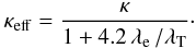 (11)This approach neglects
the influence of magnetic fields. They mainly affect dense objects like clusters of
galaxies. We focus on regions of low to intermediate density. Therefore this approximation
is sufficient for our study.
(11)This approach neglects
the influence of magnetic fields. They mainly affect dense objects like clusters of
galaxies. We focus on regions of low to intermediate density. Therefore this approximation
is sufficient for our study.
3.2. Numerical implementation
In order to compute the time evolution of the fluid governed by the equations introduced in Sect. 3.1, we developed the new simulation code evora. The code uses a regular grid of equally sized cells and evolves cell-averaged quantities over discrete time steps. Furthermore, the set of equations is split into four subproblems: hydrodynamic advection, gravitational acceleration, integration of the chemical network, and thermal conduction. These problems are solved successively at every time step, and every solver uses the quantities updated by its predecessor as its input. Here we give a brief overview of the four solvers:
- 1.
the hydrodynamic problem is solved using the well-known MUSCL scheme in combination with the MINMOD slope limiter and the approximate HLLC Riemann solver (see Toro 1999);
- 2.
the gravitational potential is computed from Poisson’s equation using Fourier transforms and Green’s function (see Hockney & Eastwood 1988);
- 3.
under the assumption of IE, the number densities are computed by iteration from Ξi = 0. In the non-IE case they are integrated self-consistently using the modified Patankar scheme (Burchard et al. 2003). In both cases the cooling and heating functions are applied to the pressure using the regular Patankar scheme (see Patankar 1980);
- 4.
thermal conduction is included into our simulations by using a central difference scheme.
 |
Fig. 1 Pancake formation without cooling, heating and thermal conduction: profiles for different redshifts. Panel A: density; Panel B: velocity; Panel C: pressure; Panel D: temperature. This simulation uses an initial amplitude of Ai = 0.02 at z = 99, a perturbation scale of L = 8 Mpc, and 16 000 grid points. |
4. One-dimensional collapse
4.1. Gravitohydrodynamics
In a first step we consider the formation of a pancake without the
inclusion of any cooling and heating or of thermal conduction. This serves as a basic
configuration to be compared with the results after successively taking into account
relevant physical processes. The configuration is initialized at z = 99
by imposing a single sinusoidal perturbation with an initial amplitude A
and a wavenumber
k = 2π / L (where
L denotes the length scale of the perturbation) with respect to the
background density of the Universe. This density distribution is then scaled to the
baryonic density using fB: 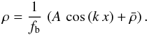 (12)According to the
linear perturbation theory (see Peebles 1993) we
obtain the corresponding velocity field
(12)According to the
linear perturbation theory (see Peebles 1993) we
obtain the corresponding velocity field
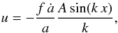 (13)where
f = (dlog D) / (dlog a),
with D denoting the growth factor. The initial temperature is set to 100
K. We always choose the size of our computational domain to be equal to the perturbation
scale L. For any of our simulations, periodic boundary conditions are
imposed.
(13)where
f = (dlog D) / (dlog a),
with D denoting the growth factor. The initial temperature is set to 100
K. We always choose the size of our computational domain to be equal to the perturbation
scale L. For any of our simulations, periodic boundary conditions are
imposed.
Before z ~ 1 the medium undergoes adiabatic contraction, resulting in a sharp density peak in the center of the box. When the local speed of sound matches the infall velocity, two shocks form and confine a region of high temperature. In Fig. 1 we show density, velocity, pressure, and temperature profiles at different redshifts after the moment of shock formation. While moving outward, infalling cold gas passes these shocks and its kinetic energy is transformed into heat. The associated strong decline in velocity is visible in the corresponding profile. As a result, the temperature inside the shocked region is several orders of magnitude higher then outside. This process is commonly called shock heating. While passing the shock, the gas looses most of its velocity and does not move further inward, but is accumulated at the outer wings of the profile, leaving the inner part unchanged. With time, a continuously decreasing fraction of matter remains outside of the shocked region. The accretion onto the pancake declines over time. This results in a slower shock speed and in a declining density profile. The final density profile bound by the shocks covers about 2.5 orders of magnitude, and is proportional to r − 2 / 3 (Shandarin & Zeldovich 1989). The pressure profile remains almost constant. This is an expected behavior since pressure gradients would be quickly erased by hydrodynamic advection. The small deviation from uniformity as well as the weak redshift dependence are the imprint of the gravitational potential and the cosmological expansion. This almost isobaric behavior can be used to explain the shape of the temperature profiles. Given a constant pressure, Eq. (8) implies an inverted behavior between temperature and density. The temperature is given in physical units implying a cosmic evolution ∝ a-2.
Without heating and cooling, the physical dimensions can be eliminated from the
hydrodynamic equations, and therefore the qualitative outcome of these simulations does
not depend on the given length scale L. If we impose a reference system
given by L, the background density of the Universe
, and the Hubble time
1 / H0, we are able to obtain scaling
relations for all quantities. For the temperature scale this yields
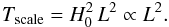 (14)Thus the temperature in
the shocked region scales as the square of the length scale of the initial perturbation.
(14)Thus the temperature in
the shocked region scales as the square of the length scale of the initial perturbation.
Besides the length scale of the perturbation, the initial amplitude is set as a parameter. Its value determines the time of caustic formation, as shown in Bryan et al. (1995). The chosen value of A = 0.02 corresponds to a shock formation at redshift z ~ 1, which could be a reasonable value for the WHIM. Owing to the cosmological expansion, the temperature declines very fast from its initial value. Therefore, the initial temperature has a negligible influence on the dynamical evolution and on the resulting profiles.
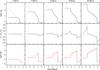 |
Fig. 2 Pancake formation including cooling and heating for an initial perturbation amplitude of A = 0.02 and for a series of perturbation scales of L = (2,8,12,16,24) Mpc/h comoving. Shown is the outcome of the simulations at z = 0 including cooling and heating (solid lines), and without dissipation (gray lines). The profiles are displayed using logarithmic coordinate axes. First row: density profiles; Second row: density flux profiles; Third row: temperature profiles. |
4.2. Cooling and heating
If cooling and heating are included into the consideration, an intrinsic physical scale
is introduced. Unlike before, the physical dimension cannot be eliminated from the
dynamical equations. Simulations using different perturbation scales L
differ not only quantitatively but also qualitatively. As a consequence, the constraint on
the ratio between the spatial resolution Δx and the local Jeans length
λJ as presented in Truelove et al. (1997) has to be fulfilled: 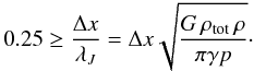 (15)If this criterion is not
fulfilled, the pressure is too weak to even out small scale perturbations, which are
caused by the finite numerical resolution. These perturbations may then grow rapidly, and
induce fragmentation for purely numerical reasons. In one-dimensional simulations this
violates the spatial symmetry of the configuration. Without the inclusion of either a
(formal) heating source or an artificial pressure floor, catastrophic cooling in the
center will appear, i.e., the density increases while the pressure decreases. This will
always result in a Jeans length that violates Eq. (15). For the one-dimensional collapse, the heating due to the UV
background is sufficient to prevent such a cooling catastrophe.
(15)If this criterion is not
fulfilled, the pressure is too weak to even out small scale perturbations, which are
caused by the finite numerical resolution. These perturbations may then grow rapidly, and
induce fragmentation for purely numerical reasons. In one-dimensional simulations this
violates the spatial symmetry of the configuration. Without the inclusion of either a
(formal) heating source or an artificial pressure floor, catastrophic cooling in the
center will appear, i.e., the density increases while the pressure decreases. This will
always result in a Jeans length that violates Eq. (15). For the one-dimensional collapse, the heating due to the UV
background is sufficient to prevent such a cooling catastrophe.
In Fig. 2 we present the outcome of our simulations including radiative cooling and heating for different length scales L of the initial perturbation. For the computation of the chemical network, we assume IE, as described in Sect. 3.1. The influence of non-IE will be discussed in Sect. 4.4. Like before, the initial amplitude is A = 0.02. With increasing L the number of grid points increases from 2000 to 64000, thus keeping a constant spatial resolution of 0.5 kpc. Displayed are the density, the density flux (instead of the velocity, because it emphasizes the high-density region in the center), and the related temperature profiles. We choose a logarithmic x-axis, thus focusing on the center of the simulation box.
As an immediate effect of the heating due to the photoionizing UV background, the configuration is heated up to temperatures of T ≈ 2 × 10⁴ K during the reionization at redshift z ≈ 6. This results in a pressure several orders of magnitudes higher than in the non-radiative simulations. Therefore, the adiabatic collapse before redshift (z ≈ 1) does not produce one single peak, but an isothermal core supported by pressure. The further evolution now depends on the size of the perturbation length scale L.
For the smallest perturbation scale L = 2 Mpc the speed of sound inside this core remains always higher than the infall velocity, and therefore the shock cannot form anymore. The whole profile, now sustained by the pressure of the gas only, is more extended than in the non-radiative case. For L > 2 Mpc the infall velocity becomes higher than the sound velocity at some moment (this can be obtained from the scaling considerations discussed above). Thus, a shock is able to form. This shock is not generated in the center, but forms at the edges of the pre-shock core. From there, it moves outward, like in the non-radiative case. Additionally, a fan-like wave penetrates into the core, effectively shrinking its size. The whole configuration can be separated into an inner isothermal core, a shocked region of higher temperatures, and an outer region at low density and low temperature. The size of the core is decreasing with increasing length scale L. Outside of the core region, the results of the simulations differ only slightly from the non-radiative case. Especially the position of the outer shock appears to be unaffected. A special situation occurs in the L = 4 Mpc simulation, where an effective outflow can be noticed, which appears as a positive density flux outside the core. This is caused by the lower density inside the core compared to the runs with higher L, resulting in longer cooling times, and thus a less effective dissipation of the energy input by the further infall.
The influence of the perturbation scale on the properties of the core will be further examined in Sect. 5.
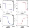 |
Fig. 3 Influence of thermal conduction is shown at regions with suficciently steep temperature gradients (L = 32 Mpc). The gray lines show the results of the corresponding simulations without thermal conduction. Panel A) and B): the density and temperature profiles at the outer shock fronts are shifted with respect to the case without heat conduction. The high-temperature region is extended outwards. The density is increased but over a lower volume (the density shock is shifted inwards). Panel C) and D): heat conduction leads to a smaller core. |
4.3. Thermal conduction
The inclusion of thermal conduction leaves an impact on the evolution of the pancake only
for perturbation scales of L ≥ 30 Mpc. The used thermal conduction
coefficient κ shows a steep temperature dependence of
κ ∝ T2.5. Moreover the temperature scales
approximately like T ∝ L2. This implies a
relatively sharp transition between perturbation scales where thermal conduction is
effective or not. Furthermore, thermal conduction is only important if steep temperature
gradients occur. This is particularly expected within the immediate neighborhood of the
shock fronts or/and for the temperature step at the core edges. Then it might occur that
the thermal heat conduction exceeds the cooling and the formed core is heated up
(evaporation). For this case, a rough order-of-magnitude estimate gives the condition
under which thermal conduction may overcome the cooling, i.e.
− ∇·j > Λ. For an estimate, we
assume an average cooling comparable with that by recombination or collisional excitation.
Then we get the relation  (16)where
ne,λT are the
electron number density and the characteristic scale for the temperature gradient,
respectively. Owing to the considerable temperature difference throughout the transition
zone, one should take T at the at the core edge, whereas for
ne one should take the value inside the core. At temperature
differences of about 106 K and ne ≈ 10-4
cm-3 we get a few kpc for the transition scale
λT.
(16)where
ne,λT are the
electron number density and the characteristic scale for the temperature gradient,
respectively. Owing to the considerable temperature difference throughout the transition
zone, one should take T at the at the core edge, whereas for
ne one should take the value inside the core. At temperature
differences of about 106 K and ne ≈ 10-4
cm-3 we get a few kpc for the transition scale
λT.
In Fig. 3 we show the details of the density and temperature profiles for one perturbation scale L = 32 Mpc. The influence of L will be further discussed in Sect. 5. The top panels show the region of the confining shock. In the simulations including thermal conduction, the shocks in density and temperature do not coincide anymore. Thermal energy from the shocked region has been transported outward, heating the domain in front of the shock to temperatures comparable to the shocked region. This energy is lost by the shocked region, resulting in a lower pressure and causing a more confined density profile. The now higher temperature in front of the shock results in a higher pressure there, slowing down the infalling gas. This deceleration causes the small increase in density adjacent to the shock.
Thermal conduction also affects the resulting core profile in the simulations including heating and cooling (see Sect. 4.2). The inner part of the pancake profile is shown in the bottom panels of Fig. 3. Now, the core is distinguished by a steep increase of the temperature at the core border of approximately one order in magnitude. There, thermal conduction transports energy toward the center of the profile. This additional energy raises the pressure in the center, causing an outflow. This results in a smaller core size with respect to the simulations without heat conduction. Contrary to the outer shock front, there is no displacement between the density and the temperature profiles. The core shrinks as a whole.
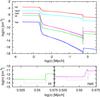 |
Fig. 4 Top panel: chemical composition of a simulated pancake (L = 32 Mpc) including cooling and heating without thermal conduction (solid lines) and with thermal conduction (dashed lines). The colors indicate different species (lines from top to bottom): red: H ii, cyan: He ii, magenta: He ii, green: H i, blue: He i; Bottom Panel: chemical composition in the region of the shock (indicated by the box in the top panel) using non-IE chemistry for H i (left) and He ii (right). The corresponding profiles from the top panel are shown in gray for comparison. [See the electronic edition of the Journal for a color version of this figure.] |
4.4. Chemical composition
Under quite general conditions, the characteristic time scales for chemical processes, e.g., such as ionization and recombination, are much shorter than the dynamical ones. Then, it is entirely justified to assume IE. The chemical composition is entirely determined by the temperature and the number densities of species engaged within the processes. In the top panel of Fig. 4 we show the number density profiles assuming IE for a perturbation scale of L = 32 Mpc (this corresponds to the results shown in the fourth column in Fig. 2). The gas is almost completely ionized, which leads to very low abundances of H i, He i, and He ii. The shapes of the profiles resemble the density profile, except for a noticeable step at the position of the shock caused by the steep decrease in temperature at this position. In the simulations including thermal conduction, the behavior at the position of the shock is even more complex: The number densities of the H i, He i, and He ii show a gap in the region adjacent to the shock. Because of the offset between the temperature shock and the density shock caused by thermal conduction (cp. with the preceding section), this region combines a low density with a high temperature, which causes a higher degree of ionization.
Under certain conditions the characteristic time scales become comparable and the assumption of ionization equilibrium may become inappropriate. This might happen at very small number densities. In this case, we have to follow the detailed evolution of the chemical network using the full set of non-IE Eqs. (6).
In those simulations, omitting the assumption of IE, the results differ only marginally from that ones of the IE-simulations. Effects on the hydrodynamic evolution, coupled by the cooling/heating function to the chemical network, cannot be detected at all. However, the chemical composition shows a slight deviation with respect to the IE simulations, and this occurs only in the direct vicinity of the shock. In the bottom panels of Fig. 4 we show the number density of H i and He ii around the shock using IE and non-IE. In the non-IE simulation a very small region adjacent to the shock exists where for He ii the degree of ionization is lower than in the IE case. The corresponding chemical timescale becomes comparable with the hydrodynamical timescale. In combination with the motion of the shock, this produces the observed behavior. Since, at the temperatures present in that region, the chemical rates for the H i are higher, the chemical time-scales are short, and a similar feature is not observed. Owing to the discussed offset between temperature shock and density shock, the chemical time scales at the shock region are even larger, which results in a more extended region of delayed ionization. The same behavior can be observed for He i, only at much lower number densities.
Though the effects of non-IE for the primordial composition are only marginal, the influence of the particular conditions at the shock position has been demonstrated. Thus for a medium containing some fraction of heavy elements which have very low densities for usual abundances, the non-IE must be taken into consideration.
If omitting the assumption of uniform temperature for all fluid components (electrons, ions) the effects on non-IE maybe much larger (Teyssier et al. 1998).
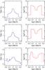 |
Fig. 5 Pancake formation if Gaussian random perturbations are taken into account for the initial density field according to the cosmological perturbation power spectrum. The resulting density (left) and temperature (right) profiles are shown at z = 0 for an initial perturbation at L = 8 Mpc. The included upper scale length for the Gaussian random perturbations as fraction of L decreases from top to bottom: First row: 1/8 L; Second row: 1/4 L; Third row: 1/2 L. The obtained profiles are compared with the single-mode consideration given in Fig. 2. The latter is shown in gray. |
4.5. Influence of small-scale perturbations
The initial conditions for cosmological simulations of large-scale structure formation are given by a spectrum of perturbations. To take this into account, we add Gaussian random perturbations according to the cosmological power spectrum to the particular perturbation given by Eq. (12). Then, in a given spatial region of size L, a pronounced pancake structure will only form if the considered initial perturbation amplitude dominates over the neighboring perturbation amplitudes at comparable scale size. Thus, we subsequently include all perturbation modes up to a scale size of (1 / 8,1 / 4,1 / 2) × L.
In Fig. 5 we show the density and temperature profiles of simulations including the small scale perturbations and cooling and heating at z = 0. Clearly, the perturbation modes at scales comparable with L have the most impact on the final profiles at z = 0. In this case most of the power from perturbation modes at neighboring scales will be added. In particular, this leads to an enhancement of the core density. The modes smaller than the actual Jeans length are erased by the heating due to the UV background. However, the magnitudes of the temperatures and their coarse profiles in the post-shock region are on the same order and the density profiles are nearly preserved.
We conclude that it is sufficient to consider only the collapse of a single (large enough) mode in order to gain coarse information on the thermal and chemical state of the structures of interest. In addition, the conservation of the system’s symmetry serves as a probe for the quality of the numerical treatment. The non-radiative simulations reproduce the earlier found analytic results with high accuracy (Shandarin & Zeldovich 1989).
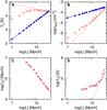 |
Fig. 6 One-dimensional collapse: dependence of various quantities on the perturbation length scale L for simulations without (•), with ( × ) cooling and heating, and with cooling and heating and thermal conduction ( + ). Panel A): central temperature (the dotted line represents Tc ∝ L-0.38; Panel B): central hydrogen number density (the dotted line represents nH ∝ L2.38); Panel C): core size (the dotted line represents λ° ∝ L-1.38); Panel D): temperature at the core boundary (the dotted line represents T° ∝ L3). In the upper panels the data points with thermal conduction are identical to those without and are therefore omitted. |
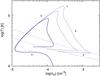 |
Fig. 7 Phase space diagram, i.e., the dependence temperature versus density, is shown for the quantities at the center of the pancake. Shown are curves for L = (16,24,32) Mpc using solid, dashed, and dotted lines, respectively. The upper gray line shows equilibrium temperature at redshift of z = 0.7 (time of shock formation) and the lower gray line at z = 0. After a period of linear growth (a), the perturbation decouples from the cosmic expansion and contracts adiabatically (b) until shock formation (at the maximum of the temperature). Then, after nearly isochoric (c) and isobaric (d) evolution stages the central gas arrives at thermal equilibrium (e). |
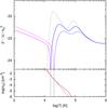 |
Fig. 8 Top panel: absolute value of the cooling/heating function
| Γ − Λ | for a hydrogen number density of
nH = 4.6 × 10⁻³ cm-3
corresponding to an overdensity of |


5. Scaling relations
In the preceding section it was shown that the length scale of the perturbation L is the determining parameter for the evolution of the pancake characteristics (temperature and density profiles). In Fig. 6 we present the L-dependence of the final values of the central temperature Tc, the central hydrogen number density nHc, the radius of the isothermal core λ°, and the temperature at its edge T°.
For the non-radiative simulations, Tc shows the expected behavior: The temperature scales ∝ L2, and thus Tc, as well. The density does not depend on L, its profile is uniquely ∝ r − 2 / 3 (see Shandarin & Zeldovich 1989). However, because we increase the number of grid points in order to keep the spatial resolution fixed, larger simulations resolve the central peak better. In the result, we get an apparent dependence of the central density, i.e., of the density at the innermost grid point, ∝ L2 / 3. However, the latter reflects only the degree of resolution.
If including cooling and heating processes, the above relations are no longer valid. The central temperature stays roughly constant at about 2 × 10⁴ K, weakly decreasing at higher L proportional to L-0.38. The central hydrogen number density shows a strong dependence on L approaching the asymptote nHc ∝ L2.38. At the edge of the isothermal core, the temperature strongly increases outwards, but then flattens again. We identify the core radius λ° as the distance from the center to the inflexion point of the temperature profile. Then the core radius shows a dependence on the scale length proportional to L-1.38.
The above mentioned scaling relations for Tc,
nHc, and λ° can be explained using
simple thermodynamical arguments. Actually, the size of the core and its density is fully
determined by conditions of hydrostatic equilibrium. In this case Euler’s equations yield
for the central pressure
pc ~ nHcφ and
Poisson’s equation yields  . Combining those two estimates
we obtain
. Combining those two estimates
we obtain  (17)Without heating the
actual pressure of the cooling gas is not able to withstand the gravity forces, and no
distinguishable core is forming in these simulations. Including heating, the pressure is
raised by several orders of magnitude during reionization at z ~ 6.
(17)Without heating the
actual pressure of the cooling gas is not able to withstand the gravity forces, and no
distinguishable core is forming in these simulations. Including heating, the pressure is
raised by several orders of magnitude during reionization at z ~ 6.
In Fig. 7 we show the path with respect to the central
point of the configuration in a phase space diagram, where the temperature
Tc is plotted against the hydrogen number density
nHc (these are physical, not super-comoving quantities). The
curve enters the shown domain at the center of the bottom of the plot, when reionization
heats the gas to ≈ 2 × 10⁴ K. From there, the density decreases at an almost
constant temperature according to the linear perturbation growth and cosmological expansion.
Then the gas dynamics decouples from the Hubble flow and follows the adiabatic
pressure-density relation  . The shock forms at the maximum
of pc and Tc. During the collapse,
the energy budget of the central region is dominated by the infalling matter and not by
cooling and heating. Therefore, the scaling relation for the pressure derived for the
non-radiative simulations p ∝ L2 also holds
here. Using this relation (and γ = 5 / 3) we obtain
scaling relations for the central density and the central temperature at the time of shock
formation (denoted by the index s):
. The shock forms at the maximum
of pc and Tc. During the collapse,
the energy budget of the central region is dominated by the infalling matter and not by
cooling and heating. Therefore, the scaling relation for the pressure derived for the
non-radiative simulations p ∝ L2 also holds
here. Using this relation (and γ = 5 / 3) we obtain
scaling relations for the central density and the central temperature at the time of shock
formation (denoted by the index s):  The
formation of the two shocks moving outwards changes the situation significantly. The energy
supply through infall vanishes, and the subsequent evolution is dominated by cooling and
heating. Nevertheless the pressure inside the shocked region, determined by the potential,
stays roughly constant, like in the case without cooling and heating. Therefore the relation
pc ∝ L2 and Eq. (17) remains valid. The efficient radiative
cooling decreases the temperature toward the equilibrium temperature
Te of the cooling/heating function, which is the temperature
where the contributions of the cooling processes and the UV background heating are canceling
each other. The gas with a higher temperature cools down toward
Te, while colder gas gets heated. In case of ionizational
equilibrium this temperature is a function of the density only. In the top panel of
Fig. 8 we show the absolute value of the normalized
cooling/heating function
The
formation of the two shocks moving outwards changes the situation significantly. The energy
supply through infall vanishes, and the subsequent evolution is dominated by cooling and
heating. Nevertheless the pressure inside the shocked region, determined by the potential,
stays roughly constant, like in the case without cooling and heating. Therefore the relation
pc ∝ L2 and Eq. (17) remains valid. The efficient radiative
cooling decreases the temperature toward the equilibrium temperature
Te of the cooling/heating function, which is the temperature
where the contributions of the cooling processes and the UV background heating are canceling
each other. The gas with a higher temperature cools down toward
Te, while colder gas gets heated. In case of ionizational
equilibrium this temperature is a function of the density only. In the top panel of
Fig. 8 we show the absolute value of the normalized
cooling/heating function  for number densities
corresponding to overdensities of 1000 and 5000 at redshift z = 0.7, which
is the approximate time of shock formation. The equilibrium temperature is given by the zero
value of
for number densities
corresponding to overdensities of 1000 and 5000 at redshift z = 0.7, which
is the approximate time of shock formation. The equilibrium temperature is given by the zero
value of  (the values in Fig. 8 are absolute values). A higher density shifts
Te toward lower temperatures. Computing
for several densities and
tracking the minimum we obtain a relation between nH
and Te. This is shown in the bottom panel of Fig. 8. This relation is also shown in Fig. 7 (solid gray lines), for both z = 0.7 and
z = 0. Evidently, when reaching Te, the
central state remains there, evolving further only due to the cosmological expansion. In the
interval of overdensities of 1000–5000 (at z = 0.7), the relation can be
approximated by a power law
(the values in Fig. 8 are absolute values). A higher density shifts
Te toward lower temperatures. Computing
for several densities and
tracking the minimum we obtain a relation between nH
and Te. This is shown in the bottom panel of Fig. 8. This relation is also shown in Fig. 7 (solid gray lines), for both z = 0.7 and
z = 0. Evidently, when reaching Te, the
central state remains there, evolving further only due to the cosmological expansion. In the
interval of overdensities of 1000–5000 (at z = 0.7), the relation can be
approximated by a power law  (indicated in
Fig. 8). At lower densities the behavior deviates
only weakly from that relation. Using this approximation and
(indicated in
Fig. 8). At lower densities the behavior deviates
only weakly from that relation. Using this approximation and  we obtain
 Although
we have only used the approximated relation for the equilibrium temperature, the above
consideration leads us to expressions that fully agree with the results shown in Fig. 6. This means that the system eventually approaches a
quasi-equilibrium state for sufficiently large scales, at least.
Although
we have only used the approximated relation for the equilibrium temperature, the above
consideration leads us to expressions that fully agree with the results shown in Fig. 6. This means that the system eventually approaches a
quasi-equilibrium state for sufficiently large scales, at least.
The core size decreases with increasing scale length L according to
λ° ∝ L-1.38. As can be seen in
Figs. 3 and 6
the heat conduction even amplifies this tendency. Thus it might be expected that for some
scale length L an evaporation of the core will happen. Obviously, that will
be the case if the core according to the cooling/heating processes becomes of comparable
size as the above introduced heat transition scale λT, i.e.
λT ≥ λ°. Using the
expression (16) and the derived scaling
relations normalized to the corresponding numerical values at L = 16 Mpc we
obtain for the scale length at which the core is significantly affected by thermal
conduction  (23)At larger scales even
evaporation of the core becomes possible. This also principally agrees with the results
obtained by Bond et al. (1984).
(23)At larger scales even
evaporation of the core becomes possible. This also principally agrees with the results
obtained by Bond et al. (1984).
6. Summary and conclusions
The aim of the present paper is to investigate the detailed physics and thermodynamics of a matter distribution which reflects the basic properties of structures of the WHIM. From cosmological simulations we know that the WHIM is distributed in sheets and filaments. For the description of a matter distribution at low density the resolution is a key issue. Therefore, we initially concentrated on the description of the one-dimensional collapse toward a gaseous sheet at extremely high resolution. Although neglecting any interaction between the perturbations on various scales we started with perturbation parameters consistent with the cosmological density field. Above an initial perturbation scale of ≈ 2 Mpc the collapsing gas shocks and further thermodynamics are mainly determined by the cooling and heating processes. In case of the one-dimensional collapse the heating by the photoionizing UV background is sufficient to keep the whole structure in a quasi-equilibrium state. Then the final density and temperature distribution depends on the initial perturbation length scale L only, i.e. all quantities characterizing the quasi-equilibrium state may be roughly described as function of that length scale L. If keeping the resolution high enough and fixed, and increasing the initial length scale L then this goes beyond the numerical capabilities. The obtained scaling relations can be used thought to extrapolate the results towards higher L.
The one-dimensional density and temperature profiles are characterized by the existence of a cold and dense core region which is at thermal equilibrium at a temperature of Tc ≈ 2 × 10⁴ K. This core is built even before shock formation, and its properties are given by the interplay between radiative cooling and the energetic input from the UV background.
In this respect the question about a possible shielding of the UV flux is essential. However, the estimates of the optical depth τph with respect to photoionization by the UV flux show for all possible cases τph ≪ 1. The situation may be different for the three-dimensional case when higher densities are reached.
The determining variable is again the perturbation scale L: larger collapsing scales lead to a spatially narrower cold region. The size of the core region decreases even more if thermal conductivity becomes efficient. For large enough scales L the temperature gradients at the transition from the cold core towards the shock heated gas are large. In the result, thermal conductivity leads to a partial “evaporation” of the core. Using the derived scaling relations with respect to the parameter L we can estimate the approximate collapse scale when the core will be entirely evaporated. In the result, we get a range of scales L between 2 and 30 Mpc, for which a cold and shock-confined core can exist.
The cold gas in the core region of the WHIM structures must contain a relatively large fraction of neutral hydrogen and should be detectable as Lyα absorption lines in the light of more distant sources. If the core size is estimated to be on the order of ≈ 10 kpc and the overdensity is in the range 100 < δ < 1000, then Lyα absorption lines could reach column densities of about NHI ≈ 1014 to 1015 cm-2. At once, a contribution in absorption or emission by the heavy element contamination in the WHIM should be detected. A likely detection of such a simultaneous event was reported recently by Nicastro et al. (2010), using combined X-ray and optical observations towards the Seyfert 1 Galaxy PKS 0558-504. Of course, the particular observation depends on the actual geometry and orientation of the filament and the line of sight. The probability for direct observations of the cold core region is rather low.
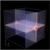 |
Fig. 9 Rendering of the density field at z = 0 for three-dimensional simulation using L = 4 Mpc. Overdensities in red, underdensities in blue [See the electronic edition of the Journal for a color version of this figure.] |
High-resolution hydrodynamical simulations on galaxy formation (Ocvirk et al. 2008; Kereš et al. 2009b,a; Agertz et al. 2009; Ceverino et al. 2010) indicate another very important aspect. At higher redshifts z = 2 − 3, relatively cold gas is flowing along the filaments toward the connected galactic halos. The cold gas streams may even reach inner galactic regions, which are closer to the center than the virial shock region. These cold gas streams may supply galaxies with fuel for star formation or may influence the the galactic star formation, at least. Several studies discuss in which way the existence of these cold streams is related to the galaxy mass. Kereš et al. (2005) find that the cold gas accretion is only important for total galactic masses ≤ 1011.4M⊙. Related estimates are given in Dekel et al. (2009). If the WHIM gas is located mainly within a network of large shock-confined filaments at z ≈ 0, then even recently a certain gas flow could be expected towards the corresponding knots of the network. Those knots could be matter concentrations of galactic or even of galaxy cluster size.
If extending our above considerations in three dimensions, multi-streaming occurs, leading to the formation of a well-defined filament and a halo, cp. Fig. 9. Though the shape of the gas distribution is extremely idealized, it is expected to exhibit the correct density and temperature profiles depending on the initial scale length, again. The large-scale gas velocities are determined by the gravitational potential. In the three-dimensional case, the velocities toward the forming filament and even more toward the halo are becoming high enough to generate shocks. Instead of a core, a relatively cold stream forms along the three-dimensional filament, propagating deep into the halo. The temperature and density profiles for the three-dimensional case are much more complex even for the highly idealized geometry. We are going to consider this in a forthcoming paper (Klar & Mücket, in prep.). However, the existence of a natural regulation mechanism for the size and existence of a cold core for the one-dimensional case might indicate similar restrictions for the cold stream in three dimensions.
Acknowledgments
J.S.K. acknowledges A. Partl, T. Doumler, S. Knollmann, A. Booley and R. Teyssier for help and useful discussions. J.S.K. was supported by the Deutsche Forschungsgemeinschaft under the project MU 1020/6-4.s and by the German Ministry for Education and Research (BMBF) under grant FKZ 05 AC7BAA.
References
- Agertz, O., Teyssier, R., & Moore, B. 2009, MNRAS, L263 [Google Scholar]
- Atrio-Barandela, F., & Mücket, J. P. 2006, ApJ, 643, 1 [NASA ADS] [CrossRef] [Google Scholar]
- Atrio-Barandela, F., Mücket, J. P., & Génova-Santos, R. 2008, ApJ, 674, L61 [NASA ADS] [CrossRef] [Google Scholar]
- Bertone, S., Schaye, J., Dal la Vecchia, C., et al. 2010, MNRAS, 407, 544 [NASA ADS] [CrossRef] [Google Scholar]
- Bianchi, S., Cristiani, S., & Kim, T. 2001, A&A, 376, 1 [NASA ADS] [CrossRef] [EDP Sciences] [Google Scholar]
- Black, J. H. 1981, MNRAS, 197, 553 [NASA ADS] [Google Scholar]
- Bond, J. R., Centrella, J., Szalay, A. S., & Wilson, J. R. 1984, MNRAS, 210, 515 [NASA ADS] [Google Scholar]
- Branchini, E., Ursino, E., Corsi, A., et al. 2009, ApJ, 697, 328 [NASA ADS] [CrossRef] [Google Scholar]
- Bryan, G. L., Norman, M. L., Stone, J. M., Cen, R., & Ostriker, J. P. 1995, Comput. Phys. Commun., 89, 149 [Google Scholar]
- Burchard, H., Deleersnijder, E., & Meister, A. 2003, Appl. Numer. Math., 47, 1 [CrossRef] [Google Scholar]
- Cen, R., & Ostriker, J. P. 1999, ApJ, 514, 1 [NASA ADS] [CrossRef] [Google Scholar]
- Cen, R., Tripp, T. M., Ostriker, J. P., & Jenkins, E. B. 2001, ApJ, 559, L5 [NASA ADS] [CrossRef] [Google Scholar]
- Ceverino, D., Dekel, A., & Bournaud, F. 2010, MNRAS, 404, 2151 [NASA ADS] [Google Scholar]
- Davé, R., Cen, R., Ostriker, J. P., et al. 2001, ApJ, 552, 473 [NASA ADS] [CrossRef] [Google Scholar]
- Dekel, A., Birnboim, Y., Engel, G., et al. 2009, Nature, 457, 451 [NASA ADS] [CrossRef] [PubMed] [Google Scholar]
- Dolag, K., Meneghetti, M., Moscardini, L., Rasia, E., & Bonaldi, A. 2006, MNRAS, 370, 656 [NASA ADS] [Google Scholar]
- Doroshkevich, A. G., & Shandarin, S. F. 1978, Soviet Astron., 22, 653 [Google Scholar]
- Doroshkevich, A. G., & Zeldovich, Y. B. 1964, Soviet Astron., 7, 615 [NASA ADS] [Google Scholar]
- Doumler, T., & Knebe, A. 2010, MNRAS, 403, 453 [NASA ADS] [CrossRef] [Google Scholar]
- Elvis, M., Nicastro, F., & Fiore, F. 2004, in COSPAR, Plenary Meeting, 35th COSPAR Scientific Assembly, 35, 563 [Google Scholar]
- Fang, T., & Canizares, C. R. 2000, ApJ, 539, 532 [NASA ADS] [CrossRef] [Google Scholar]
- Fang, T., & Bryan, G. L. 2001, ApJ, 561, L31 [NASA ADS] [CrossRef] [Google Scholar]
- Fang, T., Croft, R. A. C., Sanders, W. T., et al. 2005, ApJ, 623, 612 [NASA ADS] [CrossRef] [Google Scholar]
- Fang, T., Marshall, H. L., Lee, J. C., Davis, D. S., & Canizares, C. R. 2002, ApJ, 572, L127 [NASA ADS] [CrossRef] [Google Scholar]
- Feng, L.-L., Shu, C.-W., & Zhang, M. 2004, ApJ, 612, 1 [Google Scholar]
- Finoguenov, A., Briel, U. G., & Henry, J. P. 2003, A&A, 410, 777 [NASA ADS] [CrossRef] [EDP Sciences] [Google Scholar]
- Frigo, M., & Johnson, S. G. 2005, Proceedings of the IEEE, special issue on Program Generation, Optimization, and Platform Adaptation, 93, 216 [Google Scholar]
- Fujimoto, R., Takei, Y., Tamura, T., et al. 2004, PASJ, 56, L29 [NASA ADS] [Google Scholar]
- Génova-Santos, R., Atrio-Barandela, F., Mücket, J. P., & Klar, J. S. 2009, ApJ, 700, 447 [NASA ADS] [CrossRef] [Google Scholar]
- Gnedin, N. Y. 2000, ApJ, 535, 530 [NASA ADS] [CrossRef] [Google Scholar]
- Haardt, F., & Madau, P. 2001, in Clusters of Galaxies and the High Redshift Universe Observed in X-rays, ed. D. M. Neumann & J. T. V. Tran [Google Scholar]
- Hellsten, U., Gnedin, N. Y., & Miralda-Escudé, J. 1998, ApJ, 509, 56 [NASA ADS] [CrossRef] [Google Scholar]
- Hockney, R. W., & Eastwood, J. W. 1988, Computer simulation using particles (Bristol: Hilger) [Google Scholar]
- Jubelgas, M., Springel, V., & Dolag, K. 2004, MNRAS, 351, 423 [NASA ADS] [CrossRef] [Google Scholar]
- Kaastra, J. S., Lieu, R., Tamura, T., Paerels, F. B. S., & den Herder, J. W. 2003, A&A, 397, 445 [NASA ADS] [CrossRef] [EDP Sciences] [Google Scholar]
- Katz, N., Weinberg, D. H., & Hernquist, L. 1996, ApJS, 105, 19 [NASA ADS] [CrossRef] [Google Scholar]
- Kawahara, H., Yoshikawa, K., Sasaki, S., et al. 2006, PASJ, 58, 657 [NASA ADS] [Google Scholar]
- Kay, S. T., Pearce, F. R., Jenkins, A., et al. 2000, MNRAS, 316, 374 [NASA ADS] [CrossRef] [Google Scholar]
- Kereš, D., Katz, N., Weinberg, D. H., & Davé, R. 2005, MNRAS, 363, 2 [NASA ADS] [CrossRef] [Google Scholar]
- Kereš, D., Katz, N., Davé, R., Fardal, M., & Weinberg, D. H. 2009a, MNRAS, 396, 2332 [NASA ADS] [CrossRef] [Google Scholar]
- Kereš, D., Katz, N., Fardal, M., Davé, R., & Weinberg, D. H. 2009b, MNRAS, 395, 160 [NASA ADS] [CrossRef] [Google Scholar]
- Komatsu, E., Dunkley, J., Nolta, M. R., et al. 2009, ApJS, 180, 330 [NASA ADS] [CrossRef] [Google Scholar]
- Martel, H., & Shapiro, P. R. 1998, MNRAS, 297, 467 [NASA ADS] [CrossRef] [Google Scholar]
- Mathur, S., Weinberg, D. H., & Chen, X. 2003, ApJ, 582, 82 [NASA ADS] [CrossRef] [Google Scholar]
- Nicastro, F., Zezas, A., Drake, J., et al. 2002, ApJ, 573, 157 [NASA ADS] [CrossRef] [Google Scholar]
- Nicastro, F., Mathur, S., Elvis, M., et al. 2005a, Nature, 433, 495 [NASA ADS] [CrossRef] [PubMed] [Google Scholar]
- Nicastro, F., Mathur, S., Elvis, M., et al. 2005b, ApJ, 629, 700 [NASA ADS] [CrossRef] [Google Scholar]
- Nicastro, F., Krongold, Y., Fields, D., et al. 2010, ApJ, 715, 854 [NASA ADS] [CrossRef] [Google Scholar]
- Ocvirk, P., Pichon, C., & Teyssier, R. 2008, MNRAS, 390, 1326 [NASA ADS] [Google Scholar]
- Patankar, S. V. 1980, Numerical Heat Transfer and Fluid Flow (New York: McGraw-Hill) [Google Scholar]
- Peebles, P. J. E. 1993, Principles of physical cosmology (Princeton University Press) [Google Scholar]
- Perna, R., & Loeb, A. 1998, ApJ, 503, L135 [NASA ADS] [CrossRef] [Google Scholar]
- Prochaska, J. X., & Tumlinson, J. 2008, e-prints [arXiv:0805.4635] [Google Scholar]
- Sarazin, C. L. 1988, X-ray emission from clusters of galaxies (Cambridge University Press) [Google Scholar]
- Schaye, J., Vecchia, C. D., Booth, C. M., et al. 2009, MNRAS, 1888 [Google Scholar]
- Shandarin, S. F., & Zeldovich, Y. B. 1989, Reviews of Modern Physics, 61, 185 [Google Scholar]
- Spitzer, L. 1962, Physics of Fully Ionized Gases (New York: Interscience), 2nd ed. [Google Scholar]
- Stocke, J. T., Shull, J. M., & Penton, S. V. 2004, e-prints [arXiv:astro-ph/0407352] [Google Scholar]
- Struck-Marcell, C. 1988, PASP, 100, 1367 [NASA ADS] [CrossRef] [Google Scholar]
- Sunyaev, R. A., & Zeldovich, Y. B. 1972, A&A, 20, 189 [NASA ADS] [Google Scholar]
- Teyssier, R. 2002, A&A, 385, 337 [NASA ADS] [CrossRef] [EDP Sciences] [Google Scholar]
- Teyssier, R., Chièze, J., & Alimi, J. 1998, ApJ, 509, 62 [NASA ADS] [CrossRef] [Google Scholar]
- Toro, E. F. 1999, Riemann solvers and numerical methods for fluid dynamics, A practical introduction, 2nd ed. (Berlin: Springer) [Google Scholar]
- Tripp, T. M., Giroux, M. L., Stocke, J. T., Tumlinson, J., & Oegerle, W. R. 2001, ApJ, 563, 724 [NASA ADS] [CrossRef] [Google Scholar]
- Tripp, T. M., Savage, B. D., & Jenkins, E. B. 2000, ApJ, 534, L1 [NASA ADS] [CrossRef] [PubMed] [Google Scholar]
- Truelove, J. K., Klein, R. I., McKee, C. F., et al. 1997, ApJ, 489, L179+ [NASA ADS] [CrossRef] [Google Scholar]
- Yoshikawa, K., Yamasaki, N. Y., Suto, Y., et al. 2003, PASJ, 55, 879 [NASA ADS] [Google Scholar]
- Yoshikawa, K., Dolag, K., Suto, Y., et al. 2004, PASJ, 56, 939 [NASA ADS] [Google Scholar]
Appendix A: chemical rates and a model for the UV background
Used rates for chemical evolution, cooling, and heating.
The coefficients used to compute the evolution of the chemical network and the cooling
and heating function are shown in Table A.1. The
values of the rates of the collisional processes are taken from Katz et al. (1996), while the photoionization and photoheating rates
are taken from Black (1981). In terms of these rates
the chemical source term writes: 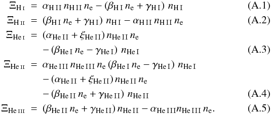 The
cooling function Λ is the sum of contributions from the collisional processes discussed
above as well as collisional excitation of H I and He II and
bremsstrahlung, while the heating function Γ is the sum of the heating rates corresponding
to the photoionization:
The
cooling function Λ is the sum of contributions from the collisional processes discussed
above as well as collisional excitation of H I and He II and
bremsstrahlung, while the heating function Γ is the sum of the heating rates corresponding
to the photoionization: 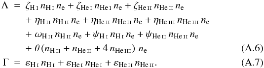 For
the computation of photoionization as well as photoheating the flux of the UV background
is needed. We use a simplified model for its redshift dependence which resembles the
current view in the literature. (Gnedin 2000; Haardt & Madau 2001; Bianchi et al. 2001):
For
the computation of photoionization as well as photoheating the flux of the UV background
is needed. We use a simplified model for its redshift dependence which resembles the
current view in the literature. (Gnedin 2000; Haardt & Madau 2001; Bianchi et al. 2001):
 (A.8)A
spectrum inversely proportional to the frequency is assumed.
(A.8)A
spectrum inversely proportional to the frequency is assumed.
Appendix B: The evora code
Most of the techniques used in our code are common in cosmological simulation codes. We will therefore concentrate on specific features of evora. To preserve readability we will give one dimensional descriptions in x direction. The generalization to three dimensions is straightforward. We will use x′ = x(t + Δt) for a quantity x after the time step Δt and x = x(t) at its beginning.
B.1. Time stepping
The length of the time step Δt is given by the minimum of three
different constraints. The first is the Courant-Friedrich-Levy condition implied by the
the hydrodynamic solver:  (B.1)where
a is the speed of sound. Moreover, the cosmological expansion during
one single time step is limited by
(B.1)where
a is the speed of sound. Moreover, the cosmological expansion during
one single time step is limited by
 (B.2)The last constraint
on the time step is associated with thermal conduction. Here, the maximal length of the
time step can be computed by estimating the fraction between the thermal energy and and
its change due to the thermal conduction:
(B.2)The last constraint
on the time step is associated with thermal conduction. Here, the maximal length of the
time step can be computed by estimating the fraction between the thermal energy and and
its change due to the thermal conduction:
 (B.3)Furthermore,
each of these time steps is further restricted by a heuristic factor
0 < C < 1. We use
Ccfl = 0.5 for the CFL-constaint,
Ca = 0.01 for the cosmological
constraint, and Ctc = 0.9 for the thermal conduction
constraint. The time steps are computed in every cell, and the minimal value is used to
compute the global time step.
(B.3)Furthermore,
each of these time steps is further restricted by a heuristic factor
0 < C < 1. We use
Ccfl = 0.5 for the CFL-constaint,
Ca = 0.01 for the cosmological
constraint, and Ctc = 0.9 for the thermal conduction
constraint. The time steps are computed in every cell, and the minimal value is used to
compute the global time step.
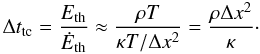
The cooling timescale (which is also the chemical timescale) can be much shorter than timescales given above. Therefore, it is not used as a constraint on the global time step. Instead we use subcycling: the time evolution of the number densities and the thermal energy density is computed using several shorter time steps. This is done locally in each cell while keeping the other quantities constant (see also Kay et al. 2000).
B.2. High Mach-number problem
In cosmological simulations, one often encounters flows of high velocity and low pressure. In these situations, the numerical computation of the difference E − Ekin, needed for the computation of the pressure, might might not yield reasonable results. This is known as the high Mach-number problem. To overcome this problem we implement the algorithm suggested by Feng et al. (2004). In addition the conservative quantities we also follow the evolution of a modified entropy density S = p / ργ − 1. In high Mach flows, where E ≈ Ekin, we use S to compute the pressure, while elsewhere E is used. After the pressure is computed the quantity not used for the computation is recomputed using p, thus keeping both quantities synchronized.
B.3. Hydrodynamic solver
If we set the right-hand side of Eqs. (1)–(4) to zero we obtain the
homogeneous Euler-equations. These equations are used to compute the pure hydrodynamic
evolution of the fluid. This problem is solved using the MUSCL-Hancock scheme as presented
in Toro (1999). To ensure the monotonicity of the
solution the MINMOD slope limiter is applied. The inter-cell fluxes are computed using a
HLLC Riemann-solver. This solver approximates the analytic solution of the Riemann problem
by three waves separating (with velocities SL,
S ⋆ , SR) four
different states: the left (L) and the right (R) initial state, and regions left
( ⋆ L) and right ( ⋆ R) of the contact discontinuity.
We use the algorithm given in Toro (1999, chap. 10.4 and
10.5) and add a prescription for the computation of the modified entropy density
and, for non-IE simulations, the number densities in the central regions
⋆ L and ⋆ R:  where
K = L or K = R for the left or right states. The wave
speeds are computed by
where
K = L or K = R for the left or right states. The wave
speeds are computed by ![\appendix \setcounter{section}{2} \begin{eqnarray} S_{\rm L} &=& \min\left[u_{\rm L} - a_{\rm L},u_{\rm R} - a_{\rm R}\right]\\ S_{\rm R} &=& \max\left[u_{\rm L} + a_{\rm L},u_{\rm R} + a_{\rm R}\right]\\ S_\star &=& \frac{p_{\rm R} - p_{\rm L} + \rho_{\rm L} u_{\rm L} \left(S_{\rm L} - u_{\rm L}\right) - \rho_{\rm R} u_{\rm R} \left(S_{\rm R} - u_{\rm R}\right)} {\rho_{\rm L} \left(S_{\rm L} - u_{\rm L}\right) - \rho_{\rm R} \left(S_{\rm R} - u_{\rm R}\right)}\cdot \end{eqnarray}](/articles/aa/full_html/2010/14/aa14040-10/aa14040-10-eq265.png) Once
the state on the interface is determined, the fluxes can be computed and the conservative
quantities can be updated.
Once
the state on the interface is determined, the fluxes can be computed and the conservative
quantities can be updated.
B.4. Gravitation
The gravitational potential is obtained though the classical algorithm used by Particle-Mesh codes. We solve Poisson’s equation with Fourier-transformations and Green’s function (Hockney & Eastwood 1988). Then, the conservative quantities are updated with the gravitational source terms. To perform the needed Fourier-transformations we use the public available FFTW library (Frigo & Johnson 2005).
B.5. Chemical evolution
The evolution of the number densities and the heating and cooling originate in the same
physical processes and have similar timescales. It is therefore necessary to compute their
evolution in a similar way. In the IE case a solution to
Ξi = 0 can be found by iteration. The situation is more
difficult in the non-IE case. Here, the integration of the system of ordinary differential
equations ṅ = Ξi is performed. These are
stiff ordinary differential equations, and therefore most codes use implicit methods for
their solution. In our code, we use a different approach and adopt the modified
Patankar scheme developed in biochemical oceanography (Burchard et al. 2003). Although it is explicit it ensures the
positivity of temperature and number densities and conserves total amount of hydrogen and
helium. The modified Euler-Patankar scheme reads: 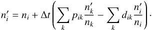 (B.9)where
pik is the production matrix containing
the rates producing species i from species k, while
dik is the destruction matrix containing
the rates that transform species i into species k. That
implies
pik = dki
and all diagonal coefficients are zero. We obtain:
(B.9)where
pik is the production matrix containing
the rates producing species i from species k, while
dik is the destruction matrix containing
the rates that transform species i into species k. That
implies
pik = dki
and all diagonal coefficients are zero. We obtain: 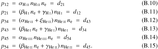 The
other components vanish. If we define
The
other components vanish. If we define
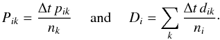 (B.16)Equation (B.9) can be further performed to
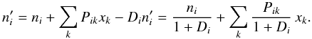 (B.17)This is an easy
solvable system of linear equations. Since the 2 × 2 block matrix for hydrogen and 3 × 3
matrix for helium are not coupled, this system can be solved for them independently.
(B.17)This is an easy
solvable system of linear equations. Since the 2 × 2 block matrix for hydrogen and 3 × 3
matrix for helium are not coupled, this system can be solved for them independently.
In the IE as well as in the non-IE case the update of the pressure is performed using
original Patankar-Trick (Patankar 1980):
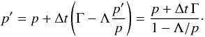 (B.18)
B.6. Thermal conduction
The algorithm for the thermal conduction is carried out similar to the hydrodynamic
scheme. After the thermal fluxes between the cells are computed, those fluxes are used to
update the energy density and modified entropy density. Like the hydrodynamic scheme this
is done in an unsplit fashion. In order to compute the thermal flux, first the temperature
gradient is computed:  (B.19)where
ix + 1 / 2 denotes the
position of the interface and ix and
ix + 1 the cell left and right of the
interface. Then, the conduction coefficient κ and the fraction of mean
free path and temperature
λe / T are computed in
cell ix and
ix + 1 and then extrapolated to the
interface ix + 1 / 2 by
simple averaging. The heat flux is then
(B.19)where
ix + 1 / 2 denotes the
position of the interface and ix and
ix + 1 the cell left and right of the
interface. Then, the conduction coefficient κ and the fraction of mean
free path and temperature
λe / T are computed in
cell ix and
ix + 1 and then extrapolated to the
interface ix + 1 / 2 by
simple averaging. The heat flux is then
 (B.20)where all quantities are
located at ix + 1 / 2. In a
final step, we update energy density and modified entropy density according to
(B.20)where all quantities are
located at ix + 1 / 2. In a
final step, we update energy density and modified entropy density according to
All Tables
All Figures
|
Fig. 1 Pancake formation without cooling, heating and thermal conduction: profiles for different redshifts. Panel A: density; Panel B: velocity; Panel C: pressure; Panel D: temperature. This simulation uses an initial amplitude of Ai = 0.02 at z = 99, a perturbation scale of L = 8 Mpc, and 16 000 grid points. |
| In the text | |
|
Fig. 2 Pancake formation including cooling and heating for an initial perturbation amplitude of A = 0.02 and for a series of perturbation scales of L = (2,8,12,16,24) Mpc/h comoving. Shown is the outcome of the simulations at z = 0 including cooling and heating (solid lines), and without dissipation (gray lines). The profiles are displayed using logarithmic coordinate axes. First row: density profiles; Second row: density flux profiles; Third row: temperature profiles. |
| In the text | |
|
Fig. 3 Influence of thermal conduction is shown at regions with suficciently steep temperature gradients (L = 32 Mpc). The gray lines show the results of the corresponding simulations without thermal conduction. Panel A) and B): the density and temperature profiles at the outer shock fronts are shifted with respect to the case without heat conduction. The high-temperature region is extended outwards. The density is increased but over a lower volume (the density shock is shifted inwards). Panel C) and D): heat conduction leads to a smaller core. |
| In the text | |
|
Fig. 4 Top panel: chemical composition of a simulated pancake (L = 32 Mpc) including cooling and heating without thermal conduction (solid lines) and with thermal conduction (dashed lines). The colors indicate different species (lines from top to bottom): red: H ii, cyan: He ii, magenta: He ii, green: H i, blue: He i; Bottom Panel: chemical composition in the region of the shock (indicated by the box in the top panel) using non-IE chemistry for H i (left) and He ii (right). The corresponding profiles from the top panel are shown in gray for comparison. [See the electronic edition of the Journal for a color version of this figure.] |
| In the text | |
|
Fig. 5 Pancake formation if Gaussian random perturbations are taken into account for the initial density field according to the cosmological perturbation power spectrum. The resulting density (left) and temperature (right) profiles are shown at z = 0 for an initial perturbation at L = 8 Mpc. The included upper scale length for the Gaussian random perturbations as fraction of L decreases from top to bottom: First row: 1/8 L; Second row: 1/4 L; Third row: 1/2 L. The obtained profiles are compared with the single-mode consideration given in Fig. 2. The latter is shown in gray. |
| In the text | |
|
Fig. 6 One-dimensional collapse: dependence of various quantities on the perturbation length scale L for simulations without (•), with ( × ) cooling and heating, and with cooling and heating and thermal conduction ( + ). Panel A): central temperature (the dotted line represents Tc ∝ L-0.38; Panel B): central hydrogen number density (the dotted line represents nH ∝ L2.38); Panel C): core size (the dotted line represents λ° ∝ L-1.38); Panel D): temperature at the core boundary (the dotted line represents T° ∝ L3). In the upper panels the data points with thermal conduction are identical to those without and are therefore omitted. |
| In the text | |
|
Fig. 7 Phase space diagram, i.e., the dependence temperature versus density, is shown for the quantities at the center of the pancake. Shown are curves for L = (16,24,32) Mpc using solid, dashed, and dotted lines, respectively. The upper gray line shows equilibrium temperature at redshift of z = 0.7 (time of shock formation) and the lower gray line at z = 0. After a period of linear growth (a), the perturbation decouples from the cosmic expansion and contracts adiabatically (b) until shock formation (at the maximum of the temperature). Then, after nearly isochoric (c) and isobaric (d) evolution stages the central gas arrives at thermal equilibrium (e). |
| In the text | |
|
Fig. 8 Top panel: absolute value of the cooling/heating function
| Γ − Λ | for a hydrogen number density of
nH = 4.6 × 10⁻³ cm-3
corresponding to an overdensity of |
| In the text | |
|
Fig. 9 Rendering of the density field at z = 0 for three-dimensional simulation using L = 4 Mpc. Overdensities in red, underdensities in blue [See the electronic edition of the Journal for a color version of this figure.] |
| In the text | |
Current usage metrics show cumulative count of Article Views (full-text article views including HTML views, PDF and ePub downloads, according to the available data) and Abstracts Views on Vision4Press platform.
Data correspond to usage on the plateform after 2015. The current usage metrics is available 48-96 hours after online publication and is updated daily on week days.
Initial download of the metrics may take a while.