| Issue |
A&A
Volume 522, November 2010
|
|
|---|---|---|
| Article Number | A105 | |
| Number of page(s) | 23 | |
| Section | Extragalactic astronomy | |
| DOI | https://doi.org/10.1051/0004-6361/200913665 | |
| Published online | 09 November 2010 | |
Rotation measures of radio sources in hot galaxy clusters⋆
1 INAF - Osservatorio Astronomico di Cagliari, Loc. Poggio dei
Pini, Strada 54, 09012 Capoterra (CA), Italy
e-mail: fgovoni@ca.astro.it
2
Max-Planck-Institut für Astrophysik, Garching, Germany
3
INAF - Istituto di Radioastronomia, via Gobetti 101,
40129
Bologna,
Italy
4
Institut für Astrophysik, Leopold-Franzens Universität Innsbruck,
Technikerstrae 25,
6020
Innsbruck,
Austria
5
Dipartimento di Astronomia, Univ. di Bologna, via Ranzani 1, 40127
Bologna,
Italy
6
Fundación Galileo Galilei - INAF, Rambla José Ana Fernández Perez
7, 38712 Breña Baja (La Palma), Canary Islands, Spain
7
Dipartimento di Astronomia, Università degli Studi di
Trieste, via Tiepolo
11, 34143
Trieste,
Italy
8 Dipartimento di Fisica, Università degli Studi di Cagliari,
Cittadella Universitaria, 09042 Monserrato (CA), Italy
Received: 13 November 2009
Accepted: 14 July 2010
Aims. The goal of this work is to investigate the Faraday rotation measure (RM) of radio galaxies in hot galaxy clusters in order to establish a possible connection between the magnetic field strength and the gas temperature of the intracluster medium.
Methods. We performed Very Large Array observations at 3.6 cm and 6 cm of two radio galaxies located in A401 and Ophiuchus, a radio galaxy in A2142, and a radio galaxy located in the background of A2065. All these galaxy clusters are characterized by high temperatures.
Results. We obtained detailed RM images at an angular resolution of 3′′ for most of the observed radio galaxies. The RM images are patchy and reveal fine substructures of a few kpc in size. Under the assumption that the radio galaxies themselves have no effect on the measured RMs, these structures indicate that the intracluster magnetic fields fluctuate down to such small scales. These new data are compared with RM information present in the literature for cooler galaxy clusters. For a fixed projected distance from the cluster center, clusters with higher temperature show a higher dispersion of the RM distributions (σRM), mostly because of the higher gas density in these clusters. Although the previously known relation between the clusters X-ray surface brightness (SX) at the radio galaxy location and σRM is confirmed, a possible connection between the σRM − SX relation and the cluster temperature, if present, is very weak. Therefore, in view of the current data, it is impossible to establish a strict link between the magnetic field strength and the gas temperature of the intracluster medium.
Key words: magnetic fields / polarization / large-scale structure of Universe / globular clusters: individual: A401 / globular clusters: individual: A2142 / globular clusters: individual: A2065
Appendix is only available in electronic form at http://www.aanda.org
© ESO, 2010
1. Introduction
The knowledge of the magnetic field properties in clusters of galaxies has significantly improved in recent years thanks to different methods of analysis (see e.g. reviews by Govoni & Feretti 2004; Feretti & Giovannini 2007; Ferrari et al. 2008, and references therein). The presence of a magnetized plasma between an observer and a radio source changes the properties of the incoming polarized emission. In particular, the position angle of the linearly polarized radiation rotates by an amount that is proportional to the path integral of the magnetic fields along the line-of-sight times the electron density of the intervening medium, i.e. the so-called Faraday rotation measure (RM).
Therefore, information on the intracluster magnetic fields can be obtained, in conjunction with X-ray observations of the hot gas, through the analysis of the RM of radio galaxies in the background or in the galaxy clusters themselves.
The RM studies of radio galaxies have been carried out on both statistical samples (e.g. Lawler & Dennison 1982; Vallée et al. 1986; Kim et al. 1990, 1991; Clarke et al. 2001) and individual galaxy clusters and galaxy groups by analyzing detailed high resolution RM images (e.g. Perley & Taylor 1991; Taylor & Perley 1993; Feretti et al. 1995, 1999a,b; Govoni et al. 2001; Taylor et al. 2001; Eilek & Owen 2002; Govoni et al. 2006; Taylor et al. 2007; Guidetti et al. 2008; Laing et al. 2008; Guidetti et al. 2010; Bonafede et al. 2010). These data are usually consistent with central magnetic field strengths of a few μG, but stronger fields, with values exceeding ≃ 10 μG, are derived in the inner regions of relaxed cooling core clusters.
For both merging and relaxed clusters, the RM distribution seen over extended radio galaxies is generally patchy, indicating that the intracluster magnetic fields are not regularly ordered, but instead they have turbulent structures on linear scales as low as 10 kpc or less.
In the last years, important progress has been made in the analysis of the magnetic field structure in galaxy clusters. In particular, it has been established that the magnetic field is likely to fluctuate over a wide range of spatial scales and, in a few galaxy clusters containing radio sources with very detailed RM images, the magnetic field power spectrum has been estimated (e.g. Enßlin & Vogt 2003; Vogt & Enßlin 2003; Murgia et al. 2004; Vogt & Enßlin 2005; Govoni et al. 2006; Guidetti et al. 2008; Laing et al. 2008; Guidetti et al. 2010; Bonafede et al. 2010).
An increasing attention is given in the literature to the connection between the magnetic field strength and the cluster gas density and temperature (e.g. Kunz et al. 2010). SPH simulations (Dolag et al. 1999, 2002, 2005a), indicated that the magnetic field intensity declines from the center of the cluster outward with a rough dependence on the thermal gas density. Such magnetic field profiles were confirmed by other simulations based on different numerical techniques (e.g. Brüggen et al. 2005; Dubois & Teyssier 2008; Collins et al. 2010). SPH simulations also predicted a very steep correlation of the mean magnetic field with the cluster temperature, e.g. B ∝ T2 (Dolag et al. 1999). However, there is also the possibility that the magnetic field strength is only mildly dependent on the cluster temperature as recently pointed out by Donnert et al. (2009). Kunz et al. (2010) predicted a dependence of the magnetic field strength on the cluster temperature in cool-core clusters ( in cool-core clusters,
  in isothermal clusters).
Dolag et al. (2001) showed that the correlation between two observable parameters, the dispersion of the RM distribution (σRM) and the cluster X-ray surface brightness in the source location (SX), is expected to reflect a correlation between the cluster magnetic field and the gas density. Indeed, measuring the slope of the σRM − SX correlation it is possible to infer the trend of the magnetic field versus the gas density. In addition, as predicted by cosmological magneto-hydrodynamic simulations (Dolag et al. 1999), galaxy clusters should have different central magnetic field strengths depending on their dynamical state and hence temperature, leading to an offset of this correlation for hot clusters.
In this work we present sensitive polarimetric Very Large Array (VLA) radio observations at multiple frequencies of polarized radio sources embedded in a set of hot, nearby clusters of galaxies. These data are compared with RM data taken from literature, in order to investigate a possible connection between the magnetic field strength and the gas temperature of the intracluster medium. Moreover, a detailed analysis of the Faraday rotation of the most interesting sources presented in this work will allow us, in a forthcoming paper, to determine the cluster magnetic field properties, by following the approach proposed in Murgia et al. (2004) and applied in the cases of A2255 (Govoni et al. 2006), A2382 (Guidetti et al. 2008), and Coma (Bonafede et al. 2010).
The paper is organized as follows: in Sect. 2 we describe the selection criteria of the targets, we illustrate the radio observations, and the data reduction. In Sect. 3 we show the results of the total intensity and polarization properties of the radio galaxies. In Sect. 4 we show the RM images. In Sect. 5 we investigate the magnetic field – gas temperature connection by comparing these new RM data and some other high quality data taken from literature with the cluster temperature. Finally, in Sect. 6 we draw the conclusions.
Throughout this paper we assume a ΛCDM cosmology with H0 = 71 kms-1 Mpc-1, Ωm = 0.27, and ΩΛ = 0.73.
2. VLA observations and data reduction
List of hot, nearby clusters of galaxies hosting the selected targets.
Details of the VLA observations.
We selected a small sample of radio galaxies embedded in a set of nearby, high temperature galaxy clusters. Starting from the X-ray flux limited sample by Edge et al. (1990), we considered all the clusters with a temperature T ≥ 8 keV, a redshift z < 0.1, and declination δ > −40° (to be observed by the VLA). Among the resulting nine clusters (Ophiuchus, Coma, A2319, A754, A2142, A401, A644, A2065, A2255) we skipped Coma and A2255 because they were already analyzed in other RM projects (Feretti et al. 1995; Govoni et al. 2006; Bonafede et al. 2010), and A754 because of its complex X-ray morphology. Of the remaining clusters, we searched in the NRAO VLA Sky Survey (NVSS; Condon et al. 1998) for bright and extended radio galaxies. We selected all the radio galaxies located within 15′ from the clusters center showing in the NVSS an angular extension LAS > 1′ and a flux density at 1.4 GHz ≥ 60 mJy. There were no radio galaxies in A644 that meet the above selection criteria. In A2319 a radio galaxy was selected, but the data were corrupted and not useful for our analysis. Thus, the final list of the new observed clusters, together with their redshift, the angular to linear conversion, the ASCA cluster temperature, and the corresponding temperature reference is given in Table 1. We note that although A2065 is reported by Edge et al. (1990) and David et al. (1993) with a high temperature, other X-ray investigation found for this cluster a temperature T < 8 keV (e.g. Markevitch 1998).
Here we present the results of multifrequency, polarimetric observations of these sources obtained with the VLA. The details of the observations are provided in Table 2. The sources were observed at 4885 MHz and 4535 MHz (4835 MHz for Ophiuchus) within the 6 cm band and at 8085 MHz and 8465 MHz within the 3.6 cm band. A401 was observed within each band in both the B and C configurations. A2142 and A2065 were observed in the B configuration within the 6 cm band and in the C configuration within the 3.6 cm band. Given its southern declination, Ophiuchus was observed with the VLA in the hybrid configurations BnA and CnB at 6 cm and 3.6 cm, respectively. All observations were made with a bandwidth of 50 MHz.
Calibration and imaging were performed with the NRAO Astronomical Image Processing System (AIPS) following the standard procedure: Fourier-Transform, Clean and Restore. Self-calibration was applied to remove residual phase variations. In the case of A401 the (u, v) data at the same frequencies but from different configurations were first handled separately and then combined.
Images of the Stokes parameters I, U, and Q have been obtained for each frequency separately. Images of polarized intensity P = (Q2 + U2)1 / 2 (corrected for the positive bias), fractional polarization FPOL = P / I and position angle of polarization Ψ = 0.5tan-1(U / Q) were derived from the I, Q, and U images.
3. Total intensity and polarization properties
In the following we give a brief description of total intensity and polarization properties of the individual sources.
For each galaxy cluster the radio contours obtained from the NVSS overlaid on the ROSAT HRI X-ray images are shown (Figs. 1, 4, 6, 8). The NVSS images are at 1.4 GHz and have an angular resolution of 45′′. The X-ray images are in the 0.1 − 2.4 keV band and have been convolved with a Gaussian with σ = 16′′. High resolution images of the radio galaxies, in the 6 cm band, overlaid on optical red plate are inset. Every radio galaxy shows an optical counterpart in the DSS21, except for A2065A which is likely a cluster background source.
In addition, for each source total intensity and polarization images at 3.6 cm and 6 cm, convolved with the same beam of 3′′, are shown (Figs. 2, 3, 5, 7, 9, 10). Contours represent total intensity while vectors represent the orientation of the projected E-field and are proportional in length to the fractional polarization. In the fractional polarization images we considered as valid pixels those where the fractional polarization FPOL was above 3σFPOL. Sample plots of the trend of the fractional polarization as a function of the observing frequencies, calculated in different regions of the sources are also shown.
We note that in some sources we found some unpolarized areas. This is likely due to a combination of sensitivity limits, small-scale tangled fields, and depolarization. The calculation of the average fractional polarization may be biased if these depolarized regions are ignored. To reduce any possible bias, we calculated the fractional polarization over the sources in all the pixels where the total intensity signal is above 5σI at all frequencies.
The relevant parameters of the I, Q, U images, convolved with a beam of 3′′, are listed in Table 3. The total flux densities, are also reported. The total flux densities were calculated, after the primary beam correction, by integrating the total intensity surface brightness, down to the noise level.
Information on total intensity and polarization images at 6 cm and 3.6 cm.
3.1. Abell 401
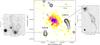 |
Fig. 1 1.4 GHz radio image of A401 obtained from the NVSS (contours) overlaid on the ROSAT HRI X-ray image (colors) in the 0.1 − 2.4 keV band. The NVSS image has an angular resolution of 45′′. The first radio contour is drawn at 1.5 mJy/beam and the rest are spaced by a factor of |

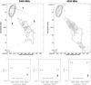 |
Fig. 2 Source A401A. Top, left: total intensity contours and polarization vectors at 3.6 cm (8465 MHz). Contour levels are drawn at: − 0.07 0.07 0.15 0.5 1 and 10 mJy/beam. Top, right: total intensity contours and polarization vectors at 6 cm (4535 MHz). Contour levels are drawn at: − 0.1 0.1 0.5 1 and 10 mJy/beam. The angular resolution is 3.0′′ × 3.0′′. The lines give the orientation of the electric vector position angle (E-field) and are proportional in length to the fractional polarization (1′′ ≃ 10%). Bottom: trend of the fractional polarization as a function of the observing frequencies, at different source locations. The depolarization DP has been calculated as the ratio of the fractional polarization between the two extreme frequencies. |
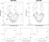 |
Fig. 3 Source A401B. Top, left: total intensity contours and polarization vectors at 3.6 cm (8465 MHz). Contour levels are drawn at: − 0.07 0.07 0.15 0.5 1 and 3 mJy/beam. Top, right: total intensity contours and polarization vectors at 6 cm (4535 MHz). Contour levels are drawn at: − 0.1 0.1 0.5 1 and 3 mJy/beam. The angular resolution is 3.0′′ × 3.0′′. The lines give the orientation of the electric vector position angle (E-field) and are proportional in length to the fractional polarization (1′′ ≃ 10%). Bottom: trend of the fractional polarization as a function of the observing frequencies, at different source locations. The depolarization DP has been calculated as the ratio of the fractional polarization between the two extreme frequencies. |
The ROSAT HRI X-ray image presented in Fig. 1 shows the X-ray emission in the 0.1 − 2.4 keV band of the cluster of galaxies A401. In the southwest, at a projected distance of about 3 Mpc, not shown in the field of view of the image, lies the A399 system. The X-ray excess and the slight temperature increase in the region between the two clusters indicate a physical link between this merging pair of clusters (e.g. Fujita et al. 1996; Fabian et al. 1997; Markevitch et al. 1998; Sakelliou & Ponmann 2004; Bourdin & Mazzotta 2008). Recent XMM X-ray analyses (Sakelliou & Ponman 2004; Bourdin & Mazzotta 2008) pointed out that neither of the two clusters contain a cooling core and their central regions are nearly isothermal, with some small-scale inhomogeneities. However, the reasonably relaxed morphology of the clusters and the absence of major temperature anomalies argue against models in which A399 and A401 have already experienced a close encounter (see also Fujita et al. 2008a).
A401 is known to contain a faint radio halo around the cD galaxy at the cluster center (Harris et al. 1980; Roland et al. 1981; Giovannini et al. 1999; Bacchi et al. 2003). We recently found (Murgia et al. 2010a) that the central region of A399 is also permeated by a diffuse low-surface brightness radio emission which we classified as radio halo. Indeed, given their proximity to each other, the interacting pair of clusters of galaxies A401 and A399 can be considered as the first example of double radio halo system.
The periphery of A401 hosts a number of tailed radio galaxies. The head-tail morphology is probably caused by a sweeping of the radio emitting material due to the relative motion between the gas and the radio galaxy. In this work we have analyzed those labeled with A401A and A401B in Fig. 1.
The distribution of spectroscopic redshifts near the pair of clusters A399 and A401 shows only one peak. This is because the velocity dispersion for individual clusters is larger than the apparent velocity separation between A401 and A399 (Hill & Oegerle 1993; Oegerle & Hill 1994; Yuan et al. 2005). On the basis of their radial velocity and their projected distance from A401, the two galaxies associated with the radio sources A401A and A401B are classified as cluster members.
A401A is located to the west of the cluster center at a projected distance of about 5.8′. The high resolution image at 6 cm reveals a peculiar morphology. A compact slightly distorted double structure of about 20′′ in size whose optical counterpart is located at RA(J2000) = 02h58m32.0s, Dec(J2000) = 13°34′20′′, and a low surface brightness tail of more than 2′ in size with a morphology which appears not directly connected to the compact emission. The total flux density of the radio galaxy, both at 6 cm and 3.6 cm, is indicated in Table 3. The compact component has a flux density of 134 ± 4 mJy and 86 ± 3 mJy at 6 cm and 3.6 cm respectively leading to a mean spectral index2α ≃ 0.7 ± 0.1, typical for radio galaxies. In the tail the spectral index is very steep (α ≃ 1.6 ± 0.1). In fact the flux density is 25 ± 1 mJy and 9.0 ± 0.3 mJy at 6 cm and 3.6 cm respectively.
The head tail A401B is located at a projected distance of about 8.5′ to the southeast of the cluster center with the head pointed versus the south of the cluster and the tail elongated versus the north. The total flux density of the radio galaxy, both at 6 cm and 3.6 cm, is indicated in Table 3. The high resolution image at 6 cm shows the core, in the position RA(J2000) = 02h59m14.9s, Dec(J2000) = 13°27′12′′, coincident with a galaxy. At 6 cm the source is about 1′ in size.
Figures 2 and 3 show the polarization images at 8465 MHz and 4535 MHz, with an angular resolution of 3′′ × 3′′.
The polarization is clearly detected at both frequencies in the bright compact double structure of A401A. The tail of A401A has a steep spectrum, consequently, the total intensity is drastically reduced at 8465 MHz and the polarized signal is detected only in the brightest regions of the tail. By considering all the pixels where the total intensity signal is above 5σI at all frequencies, the compact double structure of A401A has a mean fractional polarization of 12 ± 3% both at 8465 and 4535 MHz. In the tail the fractional polarization is higher than in the compact component reaching a mean fractional polarization of 36 ± 5% both at 8465 and 4535 MHz. In the bottom panels of Fig. 2 we show the trend of the fractional polarization as a function of the observing frequencies, at different source locations. The fractional polarization does not decrease significantly in the analyzed range of wavelengths.
A401B is polarized at both frequencies up to a distance of about 30′′. The mean fractional polarization is 20 ± 3% at 8465 and 18 ± 3% at 4535 MHz. Therefore, the depolarization is negligible. This is also confirmed in the bottom panels of Fig. 3 where we show the trend of the fraction polarization as a function of the observing frequencies, calculated in three different locations of the source.
3.2. Abell 2142
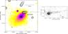 |
Fig. 4 1.4 GHz radio image of A2142 obtained from the NVSS (contours) overlaid on the ROSAT HRI X-ray image (colors) in the 0.1 − 2.4 keV band. The NVSS image has an angular resolution of 45′′. The first radio contour is drawn at 1.5 mJy/beam and the rest are spaced by a factor of |
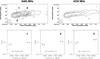 |
Fig. 5 Source A2142A. Top, left: total intensity contours and polarization vectors at 3.6 cm (8465 MHz). Contour levels are drawn at: − 0.06 0.06 0.15 0.5 and 3 mJy/beam. Top, right: total intensity contours and polarization vectors at 6 cm (4535 MHz). Contour levels are drawn at: − 0.1 0.1 0.5 1 and 3 mJy/beam. The angular resolution is 3.0′′ × 3.0′′. The lines give the orientation of the electric vector position angle (E-field) and are proportional in length to the fractional polarization (1′′ ≃ 10%). Bottom: trend of the fractional polarization as a function of the observing frequencies, at different source locations. The depolarization DP has been calculated as the ratio of the fractional polarization between the two extreme frequencies. |
The ROSAT HRI X-ray image presented in Fig. 4 shows the X-ray emission of the cooling flow cluster A2142. The cooling flow manifests itself with a cool X-ray peak as well as strong evidence for a centrally enhanced metal abundance (e.g. White et al. 1994; Peres et al. 1998). On the other hand optical (Oegerle et al. 1995) and X-ray (Henry & Briel 1996; Buote & Tsai 1996; Pierre & Starck 1998) features, such as the presence of an off-center, small scale structures and azimuthally asymmetric temperature variations, are indications of a merger. Chandra data show that the gas temperature in the central region of A2142 (Markevitch et al. 2000) is non-isothermal. It appears that the central cooling flow has been disturbed but not destroyed by the merger.
The presence of a halo in this cluster was suggested by Harris et al. (1977). Giovannini & Feretti (2000) confirmed the presence of diffuse emission, located around the brightest cluster galaxy. This source, however, is much smaller than radio halos commonly found in merging clusters and it may be a mini-halo, like those found at the center of relaxed systems (see e.g. Gitti et al. 2007; Govoni et al. 2009).
In this work we have analyzed the radio galaxy labeled with A2142A in Fig. 4. This narrow head tail radio galaxy has the head at a projected distance of about 2.7′ to the northwest of the cluster X-ray center and the tail elongated versus the west. The high resolution image at 6 cm shows the head, at the position RA(J2000) = 15h58m14.3s, Dec(J2000) = 27°16′19.5′′, coincident with a galaxy. At 6 cm the source is more than 40′′ in size. In the source we do not distinguish the two jets. A possibility is that the source is narrow because of projection effects, i.e. the radio jets are seen edge-on.
Figure 5 shows the polarization images at 8465 MHz and 4535 MHz, with an angular resolution of 3′′ × 3′′. At 8465 MHz the polarization is significant (above 3σFPOL) up to a distance of about 30′′, while at 4535 MHz the polarization signal appear below the noise level in some places along the tail. By considering all the pixels where the total intensity signal is above 5σI at all frequencies, the mean fractional polarization is 16 ± 4% at 8465 and 10 ± 3% at 4535 MHz. The source is therefore depolarized ⟨ DP ⟩ = FPOL4535 MHz / FPOL8465 MHz ≃ 0.6. The depolarization of the signal is also evident in the bottom panels of Fig. 5, where we show the trend of the fractional polarization as a function of the observing frequencies, at different source locations.
3.3. Abell 2065
 |
Fig. 6 1.4 GHz radio image of A2065 obtained from the NVSS (contours) overlaid on the ROSAT HRI X-ray image (colors) in the 0.1 − 2.4 keV band. The NVSS image has an angular resolution of 45′′. The first radio contour is drawn at 1.5 mJy/beam and the rest are spaced by a factor of |
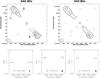 |
Fig. 7 Source A2065A. Top, left: total intensity contours and polarization vectors at 3.6 cm (8465 MHz). Contour levels are drawn at: − 0.06 0.06 0.1 0.5 and 3 mJy/beam. Top, right: total intensity contours and polarization vectors at 6 cm (4535 MHz). Contour levels are drawn at: − 0.1 0.1 0.15 3 and 6 mJy/beam. The angular resolution is 3.0′′ × 3.0′′. The lines give the orientation of the electric vector position angle (E-field) and are proportional in length to the fractional polarization (1′′ ≃ 10%). Bottom: trend of the fractional polarization as a function of the observing wavelengths, at different source locations. The depolarization DP has been calculated as the ratio of the fractional polarization between the two extreme frequencies. |
The ROSAT HRI X-ray image presented in Fig. 6 shows the X-ray emission in the 0.1 − 2.4 keV band of A2065. This is one of the galaxy clusters that make up the Corona Borealis super-cluster. The cluster X-ray surface brightness of A2065 is consistent with the optical galaxy surface-density profile, both showing elongation in the northwest – southeast direction. The cluster is a centrally condensed system with two dominant galaxies separated on the plane of the sky by 17′′ and by ≃ 600 kms-1 in redshift (Postman et al. 1988). An ASCA X-ray observation of A2065 provides evidence for an ongoing merger, but also suggests two surface brightness peaks coincident with the two central galaxies, apparently survived the merger shock passage (Markevitch et al. 1999). A Chandra observation (Chatzikos et al. 2006) reveals only one X-ray surface brightness peak, which is associated with the more luminous, southern galaxy. The gas related to that peak is cool and displaced slightly from the position of the galaxy. We note that the cluster temperature given in Table 1 (Markevitch 1998) is consistent with results from the ASCA and Chandra spectrum (White 2000; Ikebe et al. 2002; Chatzikos et al. 2006). On the other hand, David et al. (1993) derived a temperature of  , from the Einstein MPC detector.
No evidence for the presence of a cluster radio halo is available in the literature for A2065.
In this work we have analyzed the radio galaxy labeled with A2065A. It is located at a projected distance of about 13.6′ from the cluster center. The high resolution image at 6 cm, overlaid on a R-band image taken with the Telescopio Nazionale Galileo (TNG; Fig. 6), shows a radio galaxy of about 1′ in size. It shows a FRII structure, with a core located at the position RA(J2000) = 15h22m46.3s, Dec(J2000) = 27°55′40′′ and two opposite lobes, with evidence of hot-spots at the boundary of the lobes.
This radio galaxy does not show any optical counterpart in the DSS2 red image. The deeper, 30 min exposure R-band image we have taken with the TNG shows a faint source with a magnitude R = 22.0 ± 0.3. The small size of the optical counterpart in comparison with the cluster galaxies suggests that this object is a cluster background source. Moreover, if we assume that the radio source is at the cluster redshift, the estimated absolute red magnitude (with no K-correction applied) would be MR ≃ 22.0 + 5 − 5 × log 10DL(pc) = − 15.6. This is a very faint magnitude. Considering that the typical absolute magnitude of a FRII is MR = − 23.6 (e.g. Scarpa et al. 2002), the apparent magnitude of this radio source is explained if it is located at z > 1.
Figure 7 shows the polarization images at 8465 MHz and 4535 MHz, with an angular resolution of 3′′ × 3′′. The polarization has been detected in the lobes at each frequency. The two lobes have a similar fractional polarization. In the northern lobe the fractional polarization has a mean value of 16 ± 5% both at 8465 MHz and 4535 MHz, while in the southern lobe the fractional polarization has a mean value of 19 ± 5% at 8465 MHz and 17 ± 5% at 4535 MHz. The absence of depolarization is also confirmed in the bottom panels of Fig. 7 where we show the trend of the fraction polarization as a function of the observing frequencies, calculated in three different locations of the source.
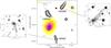 |
Fig. 8 1.4 GHz radio image of Ophiuchus obtained from the NVSS (contours) overlaid on the ROSAT HRI X-ray image (colors) in the 0.1 − 2.4 keV band. The NVSS image has an angular resolution of 45′′. The first radio contour is drawn at 1.5 mJy/beam and the rest are spaced by a factor of |
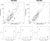 |
Fig. 9 Source OPHIB. Top, left: total intensity contours and polarization vectors at 3.6 cm (8465 MHz). Contour levels are drawn at: − 0.15 0.15 0.5 1 2 and 3 mJy/beam. Top, right: total intensity contours and polarization vectors at 6 cm (4835 MHz). Contour levels are drawn at: − 0.35 0.35 0.7 1 2 and 3 mJy/beam. The angular resolution is 3.0′′ × 3.0′′. The lines give the orientation of the electric vector position angle (E-field) and are proportional in length to the fractional polarization (1′′ ≃ 10%). Bottom: trend of the fractional polarization as a function of the observing wavelengths, at different source locations. The depolarization DP has been calculated as the ratio of the fractional polarization between the two extreme frequencies. |
3.4. Ophiuchus
Ophiuchus is a nearby, hot cluster. Suzaku data (Fujita et al. 2008b) indicate that this cluster has a cool, dense core. We recently found at the cluster center a low surface brightness diffuse emission that it is classified has a mini-halo (Govoni et al. 2009; Murgia et al. 2009, 2010b). Moreover for this cluster there have been claims of detecting hard X-ray emission in excess to the thermal emission (Eckert et al. 2008; Nevalainen et al. 2009). Such emission may be of non-thermal origin, for example, Compton scattering of relativistic electrons by the cosmic microwave background radiation (see e.g. Rephaeli et al. 2008; Petrosian et al. 2008, and references therein for recent reviews), but alternative explanations have been put forward (Profumo 2008; Pérez-Torres et al. 2009; Colafrancesco & Marchegiani 2009).
Figure 8 shows the ROSAT HRI X-ray image of the cluster overlaid on the NVSS image. In this work we have analyzed the radio galaxies labeled with OPHIB and OPHIC. In the original sets of data we observed also OPHIA (see Fig. 8), but this source is fully resolved out at both wavelengths. The lack of detection indicates that the OPHIA source is too extended to be imaged at a such small angular scale.
The source OPHIB is located to the northwest of the cluster center at a projected distance of about 14.5′. The high resolution image at 6 cm overlaid on the DSS2 red plate shows a source of about 45′′ in size with a NAT head-tail morphology. The core at the position RA(J2000) = 17h11m55.4s, Dec(J2000) = − 23°09′42.5′′ is coincident with a bright galaxy, while the tail is oriented away from the core in the northwest direction.
The NAT head-tail OPHIC is located at a projected distance of about 7.6′ to the southwest of the cluster center with the head pointed versus the cluster center and the tail elongated versus south. The high resolution image at 6 cm shows the core, at the position RA(J2000) = 17h12m09.0s, Dec(J2000) = − 23°28′26.5′′, coincident with a galaxy. At 6 cm the source is about 40′′ in size.
Figures 9 and 10 show the polarization images at 8465 MHz and 4835 MHz, with an angular resolution of 3′′ × 3′′.
OPHIB is polarized at both frequencies up to a distance of about 45′′. By considering all the pixels where the total intensity signal is above 5σI at all frequencies, the source has a mean fractional polarization of 18 ± 5% at 8465 and 22 ± 5% at 4835 MHz. Within the errors the two fractional polarizations are compatible therefore in OPHIB we do not detect significant depolarization. In the bottom panels of Fig. 9 we show the trend of the fractional polarization as a function of the observing frequencies, at different source locations.
The fractional polarization in different locations of the source OPHIC is indicated in Fig. 10. At 8465 MHz the polarization is detected only in a few places and the error on the fractional polarization is rather high. In most of the source the fractional polarization at 4835 is below the 3σFPOL level. The only patch where a significant polarization is detected has a fraction polarization compatible, within the errors, with that at 8465 MHz.
 |
Fig. 10 Source OPHIC. Left: total intensity contours and polarization vectors at 3.6 cm (8465 MHz). Contour levels are drawn at: − 0.1 0.1 0.5 1 and 2 mJy/beam. Right: total intensity contours and polarization vectors at 6 cm (4835 MHz). Contour levels are drawn at: − 0.3 0.3 0.7 2 and 3 mJy/beam. The angular resolution is 3.0′′ × 3.0′′. The lines give the orientation of the electric vector position angle (E-field) and are proportional in length to the fractional polarization (1′′ ≃ 17%). |
4. Rotation measure images
The presence of a magnetized and ionized screen between the observer and a radio source changes the properties of the incoming polarized emission. As it passes through the magnetized plasma, the polarized synchrotron radiation undergoes the following rotation of the plane of polarization:  (1)where ΨObs(λ) is the observed polarization angle at a wavelength λ and ΨInt is the intrinsic polarization angle.
The rotation measure RM is related to the plasma thermal electron density, ne, and magnetic field along the line-of-sight, B ∥ , by the equation:  (2)where B ∥ is measured in μG, ne in cm-3 and L is the depth of the screen in kpc.
Following the definition, the RM images were obtained by performing a fit of the 4 polarization angle images, at each pixel, as a function of λ2 (see Eq. (1)), by using the software FARADAY by Murgia et al. (2004). Given as input the images of Q and U, at each frequency, the software produces the RM and the intrinsic polarization angle ΨInt images, both with relative error images. To improve the RM image, the software can be iterated in several self-calibration cycles. In the first cycle only pixels with the highest signal-to-noise ratio are fitted. In the next cycles the algorithm uses the RM information in these high signal-to-noise pixels to solve the nπ-ambiguity in adjacent pixels of lower signal-to-noise, in a similar method used in the PACERMAN algorithm by Dolag et al. (2005b).
We derived the RM images, at 3′′ resolution, of the five polarized sources. They were calculated only in those pixels in which the following three conditions were satisfied: the total intensity signal at 8465 MHz was above 3σI, the error in the polarization angle at each frequency was lower than 15°, and the resulting RM error was lower than 60 rad/m2. We checked the agreement between the final RM images obtained with FARADAY and those obtained with the algorithm PACERMAN by Dolag et al. (2005b).
Figures 11 − 15 show the resulting RM images for the sources A401A, A401B, A2142A, A2065A and OPHIB, respectively. For each source the total intensity contours at 8465 MHz are overlaid on the RM images. We can characterize the RM distribution in terms of a mean ( ⟨ RM ⟩ ) and root mean square (σRM). The histograms of the RM distribution are also shown. In addition, a few plots showing the position angle ΨObs as a function of λ2 at different source locations are presented.
Rotation measure results.
In Table 4, for each radio galaxy we report its projected distance from the cluster X-ray center, the number of beams over which RMs are computed, the mean value of the RM fit error, the mean ( ⟨ RM ⟩ ) and root mean square (σRM) of the RM distribution. The errors on the ⟨ RM ⟩ and σRM quantities have been computed with Montecarlo simulations, considering both the uncertainty related to the presence of the statistical error and the fit error3.
The values of ⟨ RM ⟩ given in Table 4 are not corrected for the contribution of the Galaxy. We determined the Galactic contribution for each cluster of our sample according to the values reported in the RM catalog by Taylor et al. (2009). We used the distance-weighted mean of the RMs of all sources located within a radius of 3deg. The RM Galactic contribution in the region occupied by our cluster sample has been found to be rather small. About − 6 rad/m2 for A401, + 16 rad/m2 for A2142, and + 10 rad/m2 for A2065. While the Galactic RM is − 29 rad/m2 for Ophiuchus.
 |
Fig. 11 Rotation measure image of the radio galaxy A401A. The angular resolution is 3.0′′ × 3.0′′. The contours refer to the total intensity image at 8465 MHz. Contour levels are drawn at: 0.07 0.15 0.5 1 and 5 mJy/beam. The histogram shows the rotation measure distribution for all significant pixels. The plots show the position angle ΨObs as a function of λ2 at different source locations. |
 |
Fig. 12 Rotation measure image of the radio galaxy A401B. The angular resolution is 3.0′′ × 3.0′′. The contours refer to the total intensity image at 8465 MHz. Contour levels are drawn at: 0.07 0.15 0.5 1 and 3 mJy/beam. The histogram shows the rotation measure distribution for all significant pixels. The plots show the position angle ΨObs as a function of λ2 at different source locations. |
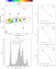 |
Fig. 13 Rotation measure image of the radio galaxy A2142A. The angular resolution is 3.0′′ × 3.0′′. The contours refer to the total intensity image at 8465 MHz. Contour levels are drawn at: 0.06 0.15 0.5 1 and 3 mJy/beam. The histogram shows the rotation measure distribution for all significant pixels. The plots show the position angle ΨObs as a function of λ2 at different source locations. |
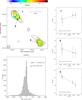 |
Fig. 14 Rotation measure image of the radio galaxy A2065A. The angular resolution is 3.0′′ × 3.0′′. The contours refer to the total intensity image at 8465 MHz. Contour levels are drawn at: 0.06 0.1 0.5 and 3 mJy/beam. The histogram shows the rotation measure distribution for all significant pixels. The plots show the position angle ΨObs as a function of λ2 at different source locations. |
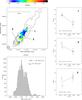 |
Fig. 15 Rotation measure image of the radio galaxy OPHIB. The angular resolution is 3.0′′ × 3.0′′. The contours refer to the total intensity image at 8465 MHz. Contour levels are drawn at: 0.15 0.5 1 2 and 3 mJy/beam. The histogram shows the rotation measure distribution for all significant pixels. The plots show the position angle ΨObs as a function of λ2 at different source locations. |
In order to verify the polarization angle linearity with λ2, we selected some pixels in different locations of the sources. The data are generally quite well represented by a linear λ2 relation. The polarization angle trend with λ2 and the absence of depolarization (at least in the case of A401, A2065, and Ophiuchus) would argue in favor of an RM produced by an external Faraday screen (Burn 1966; Laing 1984; Laing et al. 2008). However, some authors have suggested the possibility that the RM observed in radio galaxies is not associated with the foreground intracluster medium, but may arise locally to the radio source (Bicknell et al. 1990; Rudnick & Blundell 2003). A much larger λ2 range would be needed to unambiguously exclude the presence of an internal Faraday screen. However, although in this work we cannot address the origin of the screen properly (internal, external, or both), 2D Montecarlo simulations presented in the Appendix show that both RM and polarization data can be explained by the presence of a foreground Faraday screen only. In agreement with the 2D Montecarlo simulations, in the following we assume that the internal contribution is negligible and that the major factor responsible for the Faraday rotation is given by the external intracluster medium (e.g. Govoni & Feretti, and references therein). In this case, the structure of the RM images and the values of the σRM and ⟨ RM ⟩ can give information on the intracluster magnetic field structure. In particular, the RM dispersion of the histograms and the presence of small scales structure in the RM images can be explained by the fact that the cluster magnetic field fluctuates on scales smaller than the size of the sources. On the other hand, the cases of RM distributions (once corrected for the Galactic contribution) with a non-zero mean indicate that the magnetic field fluctuates also on scales larger than the radio sources. Therefore, in order to interpret correctly the RM data, magnetic field fluctuations in a wide range of spatial scales should be considered.
The radio galaxies analyzed in this work are located at a projected distance from the cluster center which range from 270 kpc (A2142A) up to 1120 kpc (A2065A).
The case of A401 is very interesting because it allows the RM to be sampled along two different lines-of-sight within the same cluster. As expected in the case of the RM being due to an external Faraday rotation due to the cluster magneto-ionized medium, the innermost source (A401A) has a higher σRM and | ⟨ RM ⟩ | than the external one (A401B). The RM images reveal patchy structures with RM fluctuations down to scales of a few kpc.
These small scale RM structures are well visible also in the other radio galaxies analyzed here. In A401A, A401B and A2142 large patches of fairly constant RM are also visible, indicating a magnetic structure fluctuating on large scales. We note however that the sampling of large scale fluctuations is rather poor.
We note that the location of Ophiuchus near the Galactic center makes this target not optimal for a magnetic field structure investigation through the RM. Therefore, the RM image of OPHIB should be considered with caution.
A2065A is a nice example of a high resolution RM image in an extended background source. Despite its distance from the cluster center, its importance is due to fact that, at least in this case, we can exclude that the patchy structures seen in the RM image are due to the turbulence locally created by the motion of the galaxy in the intracluster medium.
X-ray data of the cluster sample.
RM and X-ray data.
5. Magnetic field – gas temperature connection
The new RM data presented here increase the statistic of the RM for radio sources in hot clusters. Therefore, by comparing these new data with RM information taken from the literature it is now possible to investigate the connection between the magnetic field strength and the temperature of the intracluster medium. For a detailed statistical analysis, we formed a sample of 12 galaxy clusters for which high-quality RM data are available.
The cluster X-ray properties of the sample are presented in Table 5. For the distribution of the thermal electron gas density we assumed the standard β-model profile (Cavaliere & Fusco-Femiano 1976): 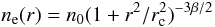 (3)where n0 and rc are the central electron density, and the cluster core radius, respectively. The X-ray parameters reported in Table 5 are taken from the literature and corrected for the cosmology adopted in this paper. The mean cluster density calculated by integrating the β-model profile over a sphere of 1 Mpc in radius is also indicated.
In the sample the temperature of the clusters is in the range T ≃ 3 − 10 keV, while the mean β-model parameters are: ⟨ β ⟩ = 0.7, ⟨ rc ⟩ = 285 kpc, and ⟨ n0 ⟩ = 4.4 × 10⁻³ cm-3. In the cluster sample there are a total of 29 radio galaxies, for which high-quality RM data are available. For each radio source, in Table 6 we report the projected distance from the cluster X-ray center, and the σRM taken from the literature. We included in this analysis only those clusters hosting radio sources for which high-resolution, extended RM images are available. We did not consider RM images of sources located at the center of cooling core clusters (e.g. Taylor et al. 2002). Indeed in our list there are a few cooling flows clusters (A2142, Ophiuchus, A2382), but in these cases the analyzed sources are located at a large projected distances from the cluster center, therefore the contribution of the dense cool core to the RM is likely to be negligible.
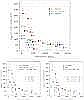 |
Fig. 16 Top: dispersion of the rotation measure distribution as a function of the projected distance from the cluster X-ray center. The different symbols represent the cluster temperature taken from the literature (red > 7 keV, green 4 − 7 keV, blue < 4 keV). Bottom: prediction of the analytical formulation by assuming a magnetic field scale ΛB = 10 kpc, and by keeping fixed the X-ray parameters to the mean values of the cluster sample β = 0.7 rc = 285 kpc. On the left n0 = 4.4 × 10⁻³ cm-3 has been fixed and we present the expectations for three different magnetic field strengths (B = 1,2,4 μG). On the right B = 3 μG has been fixed and we present the expectations for three different central gas densities (n0 = 1.5,3,6 × 10-3 cm-3). |
In Fig. 16 (top) we analyze the trend of σRM, redshift corrected by multiplying by a factor of (1 + z)2, as a function of distance from the cluster X-ray center. The different symbols represent different cluster temperature. It is evident a clear broadening of the σRM toward small projected distances, consistently with an excess of Faraday rotation due to the magnetized intracluster medium. In addition, a positive trend is found between the cluster temperature and the σRM. In particular, for a fixed projected distance from the cluster center, clusters with higher temperature show a higher σRM.
The interpretation of σRM in a cluster depends on several assumptions, including the model for the X-ray emitting gas and the magnetic field structure. To try to explain the trend between the cluster temperature and the σRM seen in Fig. 16 (top), for simplicity, we can consider an analytical formulation based on the approximation that the magnetic field is constant along the cluster and tangled on a single scale ΛB. In this simple ideal case, the screen is made of cells of uniform size, electron density and magnetic field strength, but with a field orientation at random angles in each cell. The observed RM along any given line of sight is then generated by a random walk process involving a large number of cells of size ΛB. The distribution of the RM is Gaussian with zero mean, and a variance given by:  (4)In this formulation, by considering a density distribution which follows a β-profile, the following relation (e.g. Lawler & Dennison 1982; Tribble 1991; Feretti et al. 1995; Felten 1996) for the RM dispersion is obtained by integrating Eq. (4):
  (5)where
  and Γ is the Gamma function. The constant K depends on the integration path over the gas density distribution: K = 624, if the source lies completely beyond the cluster, and K = 441 if the source is halfway the cluster. Therefore, σRM depends on the possible fluctuations in n0, B,
  and
and  . Since the linear dependence on n0 and B strongly affect σRM, in the following we concentrate on these two parameters. For most clusters of our sample, measurements of the magnetic field scale are not available from the literature. However, a discussion regarding the effect of ΛB on σRM is reported in the Appendix.
The trend seen in the top of Fig. 16, can be explained by a gas temperature − gas density relation, or by a gas temperature − magnetic field strength relation.
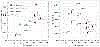 |
Fig. 17 Left: plot of the mean gas density versus the temperature of the clusters in the sample. The mean cluster density has been calculated by integrating the β-model profile over a sphere of 1 Mpc in radius. Right: plot of the core radius versus the temperature of the clusters in the sample. The different symbols represent the cluster temperature taken from the literature (red > 7 keV, green 4 − 7 keV, blue < 4 keV). |
In the bottom panels of Fig. 16 we show the predictions of the analytical formulation (Eq. (5)) obtained by assuming a magnetic field scale ΛB = 10 kpc, and by keeping fixed the X-ray parameters to the mean values of the cluster sample (β = 0.7, rc = 285 kpc). On the left bottom panel, we fixed the central gas density to n0 = 4.4 × 10⁻³ cm-3 (the mean value of the cluster sample) and we present the expectations for three different magnetic field strengths (B = 1,2,4 μG). On the right bottom panel, we fixed B = 3 μG and we present the expectations for three different central gas densities (n0 = 1.5,3,6 × 10-3 cm-3). In both cases the statistical trend of the data can be reproduced quite well. Therefore, the higher σRM in hotter clusters may be explained if they have a higher magnetic field strength and/or if they have a higher gas density.
It is not easy to disentangle the two effects; however, in the following we show that hotter clusters have higher σRM mostly because of their higher gas density. In Fig. 17 (left), we show the mean gas density plotted versus the temperature of the clusters. Clusters with a higher temperature show a higher gas density. The difference of about a factor of four in the mean density between cooler and hotter clusters may explain the difference of about a factor of four in σRM between cooler and hotter clusters. Therefore, this analysis does not confirm a strict link between the magnetic field strength and the gas temperature of the intracluster medium.
In Fig. 17 (right), we show the core radius plotted versus the temperature of the clusters. No obvious trend is present between the temperature and core radius of the clusters.
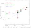 |
Fig. 18 Dispersion of the rotation measure distribution as a function of the X-ray surface brightness of the intracluster gas in the source location. The different symbols represent the cluster temperature taken from the literature (red > 7 keV, green 4 − 7 keV, blue < 4 keV). |
An alternative method to investigate a possible connection between the magnetic field strength and the gas temperature of the intracluster medium is the analysis of the σRM − SX correlation. The cluster X-ray surface brightness SX is given by: 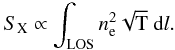 (6)The X-ray surface brightness (see Table 6) has been calculated by analyzing pointed ROSAT PSPC observations in the 0.1 − 2.4 keV band. ROSAT PSPC pointed observations were not available in the case of 3C129 and A2065 therefore we used the images taken from the ROSAT All Sky Survey, in the same band. The X-ray surface brightness has not been calculated in the location of the sources 5C4.127 and 5C4.42 (in the Coma cluster) because they are located outside the field of view of the ROSAT detector. The X-ray surface brightness (in Cts s-1 pixel-2) has been derived by averaging the X-ray count rates in an annulus comprising the position of the radio galaxies. We then corrected the count rates for the background. The background has been measured well outside the X-ray-bright cluster region. X-ray point sources have been masked out in this analysis. We finally converted the X-ray surface brightness from Cts s-1 pixel-2 to erg s-1 cm-2 sterad-1 by using the PIMMS software4. In this conversion the X-ray emission was approximated by a Raymond-Smith model with the mean cluster temperature and photoelectric absorption column density given in the literature (see Table 5).
In Fig. 18 we report the σRM − SX plot showing the trend of σRM values as a function of the cluster X-ray surface brightness SX calculated in the corresponding source location. In the plot, SX has been corrected for the dependence on the temperature by multiplying by a factor of T-0.5. In addition, SX has been corrected for the cosmological dimming of the surface brightness by dividing by a factor of (1 + z)4. The new RM data presented here (A401A, A401B, OPHIB, A2142A, A2065A) confirm the σRM − SX relation previously known in the literature (e.g. Dolag et al. 2001; Weratschnig et al. 2008). The different symbols represent different cluster temperature. As predicted by cosmological magneto-hydrodynamic simulations (Dolag et al. 1999), galaxy clusters may have different central magnetic field strengths depending on their dynamical state, leading to an offset of the σRM − SX relation, along the σRM axis, depending on the cluster temperature. An offset of the σRM − SX relation, along the σRM axis, depending on the cluster temperature if present is comparable to the intrinsic scatter of the correlation. Therefore, a possible connection between the magnetic field strength and the gas temperature, if present, is very weak. In addition, although the statistics is still limited, we note that in the σRM − SX relation clusters with extended diffuse emission (e.g. Coma, A2255, A401) seem to show a behavior similar to that of clusters without diffuse synchrotron emission.
In conclusion, present data does not permit to establish a strict link between the magnetic field strength and the gas temperature of the intracluster medium.
6. Conclusions
We performed Very Large Array observations at 3.6 cm and 6 cm of two radio galaxies located in A401 and Ophiuchus, a radio galaxy in A2142, and a radio galaxy located in the background of A2065. For most of them we obtained detailed, high resolution ( ≃ 3′′), rotation measure images. These RM images reveal patchy structures with RM fluctuations down to scales of a few kpc. Under the assumption that the radio galaxies themselves have no effect on the measured RMs, these structures indicate that the intracluster magnetic fields fluctuate down to such small scales.
These new RM data are compared with RM information taken from the literature for which similar high-resolution, extended RM images are available.
A positive trend is found between the cluster temperature and the dispersion of the RM distributions (σRM). The correlation found between the gas density and the gas temperature indicates that in our sample hotter clusters have higher σRM mostly because of their higher gas density. Moreover, although the previously known relation between the clusters X-ray surface brightness (SX) at the radio galaxy location and σRM is confirmed, a possible offset of the σRM − SX relation along the σRM axis, depending on the cluster temperature, if present is comparable to the intrinsic scatter of the correlation.
Therefore, in view of the current data it is not possible to establish a strict link between the magnetic field strength and the gas temperature of the intracluster medium.
Online material
Appendix A: : Rotation measure and depolarization in a foreground Faraday screen
Under the assumption that the RM spatial variations seen in the presented work are fully explained by external patchy screens, we investigated if these RM structural information are consistent with the observed depolarization levels at longer wavelengths. Indeed, the most direct consequence arising from RM structures which fluctuate on small scales is the beam depolarization effect.
We performed this analysis through the software FARADAY (Murgia et al. 2004). In particular we performed 2D Montecarlo simulations by assuming for the rotation measure a simple power law power spectrum of the type:  (A.1)For each source we simulated RM images by keeping fixed n = 11 / 3, corresponding to the Kolmogorov power law index for the parent magnetic field power spectrum, and by varying the minimum and maximum scale of the RM fluctuations (Λmin, Λmax). The computational grid was 1024 × 1024 pixel2 and the pixel-size was fixed to 1 kpc. The resulting field of view was then ~ 1024 × 1024 kpc2, that was enough to recover the projected size of the sources and to properly sample the RM power spectrum scales. We then added to the simulated RM images a Gaussian noise having σnoise = Errfit, in order to mimic the effect of the noise in the observed RM images and we then added an RM offset corresponding to the RM Galactic contribution in the sources location. Finally, the simulated RM images were convolved with a Gaussian function having FWHM equal to the beam of the observations, and blanked as the observations.
We performed several 2D simulations of synthetic RM images to evaluate the range of Λmin − Λmax which could explain the observed RM images. Figure A.1 (left panels) shows some examples of simulated RM images, which we found to reproduce quite well the observed RM distributions.
To quantify the two dimensional fluctuations of RM and to compare the simulations with the observations, we used the structure function as a statistical tool. The RM structure function is defined by ![\appendix \setcounter{section}{1} \begin{equation} S({\rm d}x,{\rm d}y)=\langle [{\rm RM}(x,y)-{\rm RM}(x+{\rm d}x,y+{\rm d}y)]^2\rangle_{(x,y)}, \end{equation}](/articles/aa/full_html/2010/14/aa13665-09/aa13665-09-eq199.png) (A.2)where = ⟨ ⟩ (x,y) indicates that the average is taken over all the positions (x,y) in the RM image. Blank pixels were not considered in the statistics. The structure function S(r) was then computed by radially averaging S(dx,dy) over regions of increasing size of radius
(A.2)where = ⟨ ⟩ (x,y) indicates that the average is taken over all the positions (x,y) in the RM image. Blank pixels were not considered in the statistics. The structure function S(r) was then computed by radially averaging S(dx,dy) over regions of increasing size of radius  . In the middle panels of Fig. A.1 we compare the observed (black points) and the simulated (grey-dashed) RM structure function.
In the case of an external Faraday screen, a reduction of the fractional polarization at longer wavelengths is expected if the minimum scale of the RM fluctuation (Λmin) extend to small scales (beam depolarization). Once a good representation of the RM structures have been found, we investigated the expected beam depolarization to check the consistency with the observed polarization at different wavelengths. In particular, we produced, at each observing frequency, the expected Q and U images corresponding to the simulated RM, and we taken into account the beam depolarization effects by convolving Q and U to the appropriate resolution. The predicted and observed mean degrees of polarization are then compared.
For each source we found a combination of model parameters Λmin, Λmax that gives a reasonable representation of the RM structure across the source as well as of the depolarization at longer wavelengths. The values of Λmin and Λmax we found for these sources are consistent with those found in the literature for a few other galaxy clusters (e.g. Murgia et al. 2004; Govoni et al. 2006; Guidetti et al. 2008; Bonafede et al. 2010). Therefore, even if we cannot exclude a possible presence of an internal contribution to the observed RM images, the 2D Montecarlo simulations indicate that both RM and polarization data can be explained by the presence of a foreground Faraday screen.
The different magnetic field scales ΛB of the clusters can be compared by calculating the magnetic field autocorrelation length, which takes into account the minimun and maximum scale of fluctuations (Λmin, Λmax), and the index of the power spectrum (n). Following the magnetic field autocorrelation length formula presented by Enßlin & Vogt (2003), for the new data analyzed here we found a magnetic field autocorrelation length variation of a factor of 9. This difference may influence the σRM values of about factor of 3 ( ). However, we note that the exact determination of the magnetic field power spectrum is beyond the scope of this paper, and the numbers indicated in the caption of Fig. A.1 should be considered as indicative.
 |
Fig. A.1 Left: examples of simulated RM images for the sources A401A, A401B, A2142, A2065, OPHIB. The simulated images have the same colour scale and resolution of the observed RM images. They have been obtained by simulating a RM power spectrum with a spectral index n = 11 / 3 and a minimum scale of the RM fluctuations Λmin = 5 kpc. The maximum scale of the RM fluctuations is Λmax = 205 kpc for A401A and A2142, Λmax = 128 kpc for A401B, Λmax = 15 kpc for OPHIB and A2065. Middle: structure functions of the simulated (grey) and observed (black points) RM images. Right: depolarization plots of the simulations (grey) and observations (black points). The depolarization is defined as DP(ν) = FPOLν / FPOL8465 MHz. |
Indeed, our data suffer from two kinds of uncertainty. The first source of error is related to the fit of the λ2-law and takes into account the presence of errors in the measurements of Q and U. The fit error has the effect to broad the histogram of the RM distribution and thus to increase the observed σRM. While the second uncertainty is the statistical error. The statistical errors for ⟨ RM ⟩ and for σRM is given by  and
and  respectively, where N is the number of beams over which the RM has been computed. Through the Montecarlo procedure we checked that the fit error is negligible with respect to the statistical error.
Acknowledgments
We are grateful to the referee for very useful comments that improved this paper. We would like to thank Julia Weratschnig for helpful discussions. This research was partially supported by ASI-INAF I/088/06/0 – High Energy Astrophysics and PRIN-INAF 2007. K.D. acknowledges the supported by the DFG Priority Programme 1177. The National Radio Astronomy Observatory (NRAO) is a facility of the National Science Foundation, operated under cooperative agreement by Associated Universities, Inc. This research has made use of the NASA/IPAC Extragalactic Data Base (NED) which is operated by the JPL, California Institute of Technology, under contract with the National Aeronautics and Space Administration.
References
- Bacchi, M., Feretti, L., Giovannini, G., & Govoni, F. 2003, A&A, 400, 465 [NASA ADS] [CrossRef] [EDP Sciences] [Google Scholar]
- Bicknell, G. V., Cameron, R. A., & Gingold, R. A. 1990, ApJ, 357, 373 [NASA ADS] [CrossRef] [Google Scholar]
- Bonafede, A., Feretti, L., Murgia, M., et al. 2010, A&A, 513, A30 [NASA ADS] [CrossRef] [EDP Sciences] [Google Scholar]
- Bourdin, H., & Mazzotta, P. 2008, A&A, 479, 307 [NASA ADS] [CrossRef] [EDP Sciences] [Google Scholar]
- Brüggen, M., Ruszkowski, M., Simionescu, A., Hoeft, M., & Dal la Vecchia, C. 2005, ApJ, 631, L21 [NASA ADS] [CrossRef] [Google Scholar]
- Buote, D. A., & Tsai, J. C. 1996, ApJ, 458, 27 [NASA ADS] [CrossRef] [Google Scholar]
- Burn, B. J. 1966, MNRAS, 133, 67 [NASA ADS] [CrossRef] [Google Scholar]
- Chatzikos, M., Sarazin, C. L., & Kempner, J. C. 2006, ApJ, 643, 751 [NASA ADS] [CrossRef] [Google Scholar]
- Chen, Y., Reiprich, T. H., Böhringer, H., Ikebe, Y., & Zhang, Y.-Y. 2007, A&A, 466, 805 [NASA ADS] [CrossRef] [EDP Sciences] [Google Scholar]
- Clarke, T. E., Kronberg, P. P., & Böhringer, H. 2001, ApJ, 547, L111 [NASA ADS] [CrossRef] [Google Scholar]
- Cavaliere, A., & Fusco-Femiano, R. 1976, A&A, 49, 137 [NASA ADS] [Google Scholar]
- Colafrancesco, S., & Marchegiani, P. 2009, A&A, 502, 711 [Google Scholar]
- Collins, D. C., Xu, H., Norman, M. L., Li, H., & Li, S. 2010, ApJS, 186, 308 [NASA ADS] [CrossRef] [Google Scholar]
- Condon, J. J., Cotton, W. D., Greisen, E. W., et al. 1998, AJ, 115, 1693 [NASA ADS] [CrossRef] [Google Scholar]
- David, L. P., Slyz, A., Jones, C., et al. 1993, ApJ, 412, 479 [NASA ADS] [CrossRef] [Google Scholar]
- Dolag, K., Bartelmann, M., & Lesch, H. 1999, A&A, 348, 351 [NASA ADS] [Google Scholar]
- Dolag, K., Schindler, S., Govoni, F., & Feretti, L. 2001, A&A, 378, 777 [NASA ADS] [CrossRef] [EDP Sciences] [Google Scholar]
- Dolag, K., Bartelmann, M., & Lesch, H. 2002, A&A, 387, 383 [NASA ADS] [CrossRef] [EDP Sciences] [Google Scholar]
- Dolag, K., Grasso, D., Springel, V., & Tkachev, I. 2005a, J. Cosmol. Astro-Part. Phys., 1, 9 [Google Scholar]
- Dolag, K., Vogt, C., & Enßlin, T. A. 2005b, MNRAS, 358, 726 [NASA ADS] [CrossRef] [Google Scholar]
- Donnert, J., Dolag, K., Lesch, H., & Müller, E. 2009, MNRAS, 392, 1008 [NASA ADS] [CrossRef] [Google Scholar]
- Dubois, Y., & Teyssier, R. 2008, A&A, 482, L13 [NASA ADS] [CrossRef] [EDP Sciences] [Google Scholar]
- Ebeling, H., Voges, W., Bohringer, H., et al. 1996, MNRAS, 281, 799 [NASA ADS] [CrossRef] [Google Scholar]
- Eckert, D., Produit, N., Paltani, S., et al. 2008, A&A, 479, 27 [NASA ADS] [CrossRef] [EDP Sciences] [Google Scholar]
- Edge, A. C., & Stewart, G. C. 1991, MNRAS, 252, 414 [NASA ADS] [CrossRef] [Google Scholar]
- Edge, A. C., Stewart, G. C., Fabian, A. C., & Arnaud, K. A. 1990, MNRAS, 245, 559 [NASA ADS] [Google Scholar]
- Eilek, J. A., & Owen, F. N. 2002, ApJ, 567, 202 [NASA ADS] [CrossRef] [Google Scholar]
- Enßlin, T. A., & Vogt, C. 2003, A&A, 401, 835 [NASA ADS] [CrossRef] [EDP Sciences] [Google Scholar]
- Fabian, A. C., Peres, C. B., & White, D. A. 1997, MNRAS, 285, L35 [NASA ADS] [CrossRef] [Google Scholar]
- Felten, J. E. 1996, Clusters, Lensing, and the Future of the Universe, 88, 271 [Google Scholar]
- Feretti, L., & Giovannini, G. 2007, Panchromatic View of Clusters of Galaxies and the Large-Scale Structure, ed. M. Plionis, O. Lopez-Cruz, & D. Hughes, Springer Lecture Notes in Physics, to be published [arXiv:astro-ph/0703494] [Google Scholar]
- Feretti, L., Dallacasa, D., Giovannini, G., & Tagliani, A. 1995, A&A, 302, 680 [NASA ADS] [Google Scholar]
- Feretti, L., Dallacasa, D., Govoni, F., et al. 1999a, A&A, 344, 472 [NASA ADS] [Google Scholar]
- Feretti, L., Perley, R., Giovannini, G., & Andernach, H. 1999b, A&A, 341, 29 [NASA ADS] [Google Scholar]
- Ferrari, C., Govoni, F., Schindler, S., et al. 2008, Space Sci. Rev., 134, 93 [NASA ADS] [CrossRef] [Google Scholar]
- Fujita, Y., Koyama, K., Tsuru, T., & Matsumoto, H. 1996, PASJ, 48, 191 [NASA ADS] [Google Scholar]
- Fujita, Y., Tawa, N., Hayashida, K., et al. 2008a, PASJ, 60, 343 [Google Scholar]
- Fujita, Y., Hayashida, K., Nagai, M, et al. 2008b, PASJ, 60, 1133 [NASA ADS] [Google Scholar]
- Fukazawa, Y., Makishima, K., Tamura, T., et al. 1998, PASJ, 50, 187 [NASA ADS] [Google Scholar]
- Giovannini, G., & Feretti, L. 2000, New Astron., 5, 335 [NASA ADS] [CrossRef] [Google Scholar]
- Giovannini, G., Tordi, M., & Feretti, L. 1999, New Astron., 4, 141 [NASA ADS] [CrossRef] [Google Scholar]
- Gitti, M., Ferrari, C., Domainko, W., Feretti, L., & Schindler, S. 2007, A&A, 470, L25 [NASA ADS] [CrossRef] [EDP Sciences] [Google Scholar]
- Govoni, F., & Feretti, L. 2004, Int. J. Mod. Phys. D, 13, 1549 [NASA ADS] [CrossRef] [Google Scholar]
- Govoni, F., Taylor, G. B., Dallacasa, D., et al. 2001, A&A, 379, 807 [NASA ADS] [CrossRef] [EDP Sciences] [Google Scholar]
- Govoni, F., Murgia, M., Feretti, L., et al. 2006, A&A, 460, 425 [NASA ADS] [CrossRef] [EDP Sciences] [Google Scholar]
- Govoni, F., Murgia, M., Markevitch, M., et al. 2009, A&A, 499, 371 [NASA ADS] [CrossRef] [EDP Sciences] [Google Scholar]
- Guidetti, D., Murgia, M., Govoni, F., et al. 2008, A&A, 483, 699 [NASA ADS] [CrossRef] [EDP Sciences] [Google Scholar]
- Guidetti, D., Laing, R. A., Murgia, M., et al. 2010, A&A, 514, A50 [NASA ADS] [CrossRef] [EDP Sciences] [Google Scholar]
- Harris, D. E., Bahcall, N. A., & Strom, R. G. 1977, A&A, 60, 27 [NASA ADS] [Google Scholar]
- Harris, D. E., Kapahi, V. K., & Ekers, R. D. 1980, A&AS, 39, 215 [Google Scholar]
- Henry, J. P., & Briel, U. G. 1996, ApJ, 472, 137 [NASA ADS] [CrossRef] [Google Scholar]
- Hill, J. M., & Oegerle, W. R. 1993, AJ, 106, 831 [NASA ADS] [CrossRef] [Google Scholar]
- Ikebe, Y., Reiprich, T. H., Böhringer, H., et al. 2002, A&A, 383, 773 [NASA ADS] [CrossRef] [EDP Sciences] [Google Scholar]
- Kalberla, P. M. W., Burton, W. B., Hartmann, D., et al. 2005, A&A, 440, 775 [NASA ADS] [CrossRef] [EDP Sciences] [Google Scholar]
- Kim, K. T., Kronberg, P. P., Dewdney, P. E., & Landecker, T. L. 1990, ApJ, 355, 29 [NASA ADS] [CrossRef] [Google Scholar]
- Kim, K. T., Tribble, P. C., & Kronberg, P. P. 1991, ApJ, 379, 80 [NASA ADS] [CrossRef] [Google Scholar]
- Kunz, M. W., Schekochihin, A. A., Cowley, S. C., Binney, J. J., & Sanders, J. S. 2010, MNRAS, submitted [arXiv:1003.2719] [Google Scholar]
- Laing, R. A. 1984, Physics of Energy Transport in Extragalctic Radio Sources, 90 [Google Scholar]
- Laing, R. A., Bridle, A. H., Parma, P., & Murgia, M. 2008, MNRAS, 391, 521 [NASA ADS] [CrossRef] [Google Scholar]
- Lawler, J. M., & Dennison, B. 1982, ApJ, 252, 81 [NASA ADS] [CrossRef] [Google Scholar]
- Markevitch, M. 1998, ApJ, 504, 27 [NASA ADS] [CrossRef] [Google Scholar]
- Markevitch, M., Forman, W. R., Sarazin, C. L., & Vikhlinin, A. 1998, ApJ, 503, 77 [NASA ADS] [CrossRef] [Google Scholar]
- Markevitch, M., Sarazin, C. L., & Vikhlinin, A. 1999, ApJ, 521, 526 [Google Scholar]
- Markevitch, M., Ponman, T. J., Nulsen, P. E. J., et al. 2000, ApJ, 541, 542 [NASA ADS] [CrossRef] [Google Scholar]
- Murgia, M., Govoni, F., Feretti, L., et al. 2004, A&A, 424, 429 [NASA ADS] [CrossRef] [EDP Sciences] [Google Scholar]
- Murgia, M., Govoni, F., Markevitch, M., et al. 2009, A&A, 499, 679 [NASA ADS] [CrossRef] [EDP Sciences] [Google Scholar]
- Murgia, M., Govoni, F., Feretti, L., & Giovannini, G. 2010a, A&A, 509, 86 [Google Scholar]
- Murgia, M., Eckert, D., Govoni, F., et al. 2010b, A&A, 514, A76 [NASA ADS] [CrossRef] [EDP Sciences] [Google Scholar]
- Nevalainen, J., Eckert, D., Kaastra, J., et al. 2009, A&A, 508, 1161 [NASA ADS] [CrossRef] [EDP Sciences] [Google Scholar]
- Oegerle, W. R., & Hill, J. M. 1994, AJ, 107, 857 [NASA ADS] [CrossRef] [Google Scholar]
- Oegerle, W. R., Hill, J. M., & Fitchett, M. J. 1995, AJ, 110, 32 [NASA ADS] [CrossRef] [Google Scholar]
- Peres, C. B., Fabian, A. C., Edge, A. C., et al. 1998, MNRAS, 298, 416 [NASA ADS] [CrossRef] [Google Scholar]
- Pérez-Torres, M. A., Zandanel, F., Guerrero, M. A., et al. 2009, MNRAS, 396, 2237 [NASA ADS] [CrossRef] [Google Scholar]
- Perley, R. A., & Taylor, G. B. 1991, AJ, 101, 1623 [NASA ADS] [CrossRef] [Google Scholar]
- Petrosian, V., Bykov, A., & Rephaeli, Y. 2008, Space Sci. Rev., 134, 191 [Google Scholar]
- Pierre, M., & Starck, J.-L. 1998, A&A, 330, 801 [NASA ADS] [Google Scholar]
- Postman, M., Geller, M. J., & Huchra, J. P. 1988, AJ, 95, 267 [NASA ADS] [CrossRef] [Google Scholar]
- Profumo, S. 2008, Am. Inst. Phys. Conf. Ser., 1078, 551 [Google Scholar]
- Rephaeli, Y., Nevalainen, J., Ohashi, T., & Bykov, A. M. 2008, Space Sci. Rev., 134, 71 [Google Scholar]
- Roland, J., Sol, H., Pauliny-Toth, I., & Witzel, A. 1981, A&A, 100, 7 [NASA ADS] [Google Scholar]
- Rudnick, L., & Blundell, K. M. 2003, ApJ, 588, 143 [NASA ADS] [CrossRef] [Google Scholar]
- Sakelliou, I., & Ponman, T. J. 2004, MNRAS, 351, 1439 [NASA ADS] [CrossRef] [Google Scholar]
- Scarpa, R., Govoni, F., Falomo, R., & Fasano, G. 2002, New Astron. Rev., 46, 353 [NASA ADS] [CrossRef] [Google Scholar]
- Taylor, G. B., & Perley, R. A. 1993, ApJ, 416, 554 [NASA ADS] [CrossRef] [Google Scholar]
- Taylor, G. B., Govoni, F., Allen, S., & Fabian, A. C. 2001, MNRAS, 326, 2 [NASA ADS] [CrossRef] [Google Scholar]
- Taylor, G. B., Fabian, A. C., & Allen, S. W. 2002, MNRAS, 334, 769 [NASA ADS] [CrossRef] [Google Scholar]
- Taylor, G. B., Fabian, A. C., Gentile, G., et al. 2007, MNRAS, 382, 67 [NASA ADS] [CrossRef] [Google Scholar]
- Taylor, A. R., Stil, J. M., & Sunstrum, C. 2009, ApJ, 702, 1230 [NASA ADS] [CrossRef] [Google Scholar]
- Tribble, P. C. 1991, MNRAS, 250, 726 [NASA ADS] [CrossRef] [Google Scholar]
- Vallée, J. P., MacLeod, M. J., & Broten, N. W. 1986, A&A, 156, 386 [NASA ADS] [Google Scholar]
- Vogt, C., & Enßlin, T. A. 2003, A&A, 412, 373 [NASA ADS] [CrossRef] [EDP Sciences] [Google Scholar]
- Vogt, C., & Enßlin, T. A. 2005, A&A, 434, 67 [NASA ADS] [CrossRef] [EDP Sciences] [Google Scholar]
- Weratschnig, J., Gitti, M., Schindler, S., & Dolag, K. 2008, A&A, 490, 537 [NASA ADS] [CrossRef] [EDP Sciences] [Google Scholar]
- White, D. A. 2000, MNRAS, 312, 663 [NASA ADS] [CrossRef] [Google Scholar]
- White, R. E. III,Day, C. S. R., Hatsukade, I., & Hughes, J. P. 1994, ApJ, 433, 583 [NASA ADS] [CrossRef] [Google Scholar]
- Yuan, Q.-R., Yan, P.-F., Yang, Y.-B., & Zhou, X. 2005, Chin. J. Astron. Astrophys., 5, 126 [NASA ADS] [CrossRef] [Google Scholar]
All Tables
All Figures
|
Fig. 1 1.4 GHz radio image of A401 obtained from the NVSS (contours) overlaid on the ROSAT HRI X-ray image (colors) in the 0.1 − 2.4 keV band. The NVSS image has an angular resolution of 45′′. The first radio contour is drawn at 1.5 mJy/beam and the rest are spaced by a factor of |
| In the text | |
|
Fig. 2 Source A401A. Top, left: total intensity contours and polarization vectors at 3.6 cm (8465 MHz). Contour levels are drawn at: − 0.07 0.07 0.15 0.5 1 and 10 mJy/beam. Top, right: total intensity contours and polarization vectors at 6 cm (4535 MHz). Contour levels are drawn at: − 0.1 0.1 0.5 1 and 10 mJy/beam. The angular resolution is 3.0′′ × 3.0′′. The lines give the orientation of the electric vector position angle (E-field) and are proportional in length to the fractional polarization (1′′ ≃ 10%). Bottom: trend of the fractional polarization as a function of the observing frequencies, at different source locations. The depolarization DP has been calculated as the ratio of the fractional polarization between the two extreme frequencies. |
| In the text | |
|
Fig. 3 Source A401B. Top, left: total intensity contours and polarization vectors at 3.6 cm (8465 MHz). Contour levels are drawn at: − 0.07 0.07 0.15 0.5 1 and 3 mJy/beam. Top, right: total intensity contours and polarization vectors at 6 cm (4535 MHz). Contour levels are drawn at: − 0.1 0.1 0.5 1 and 3 mJy/beam. The angular resolution is 3.0′′ × 3.0′′. The lines give the orientation of the electric vector position angle (E-field) and are proportional in length to the fractional polarization (1′′ ≃ 10%). Bottom: trend of the fractional polarization as a function of the observing frequencies, at different source locations. The depolarization DP has been calculated as the ratio of the fractional polarization between the two extreme frequencies. |
| In the text | |
|
Fig. 4 1.4 GHz radio image of A2142 obtained from the NVSS (contours) overlaid on the ROSAT HRI X-ray image (colors) in the 0.1 − 2.4 keV band. The NVSS image has an angular resolution of 45′′. The first radio contour is drawn at 1.5 mJy/beam and the rest are spaced by a factor of |
| In the text | |
|
Fig. 5 Source A2142A. Top, left: total intensity contours and polarization vectors at 3.6 cm (8465 MHz). Contour levels are drawn at: − 0.06 0.06 0.15 0.5 and 3 mJy/beam. Top, right: total intensity contours and polarization vectors at 6 cm (4535 MHz). Contour levels are drawn at: − 0.1 0.1 0.5 1 and 3 mJy/beam. The angular resolution is 3.0′′ × 3.0′′. The lines give the orientation of the electric vector position angle (E-field) and are proportional in length to the fractional polarization (1′′ ≃ 10%). Bottom: trend of the fractional polarization as a function of the observing frequencies, at different source locations. The depolarization DP has been calculated as the ratio of the fractional polarization between the two extreme frequencies. |
| In the text | |
|
Fig. 6 1.4 GHz radio image of A2065 obtained from the NVSS (contours) overlaid on the ROSAT HRI X-ray image (colors) in the 0.1 − 2.4 keV band. The NVSS image has an angular resolution of 45′′. The first radio contour is drawn at 1.5 mJy/beam and the rest are spaced by a factor of |
| In the text | |
|
Fig. 7 Source A2065A. Top, left: total intensity contours and polarization vectors at 3.6 cm (8465 MHz). Contour levels are drawn at: − 0.06 0.06 0.1 0.5 and 3 mJy/beam. Top, right: total intensity contours and polarization vectors at 6 cm (4535 MHz). Contour levels are drawn at: − 0.1 0.1 0.15 3 and 6 mJy/beam. The angular resolution is 3.0′′ × 3.0′′. The lines give the orientation of the electric vector position angle (E-field) and are proportional in length to the fractional polarization (1′′ ≃ 10%). Bottom: trend of the fractional polarization as a function of the observing wavelengths, at different source locations. The depolarization DP has been calculated as the ratio of the fractional polarization between the two extreme frequencies. |
| In the text | |
|
Fig. 8 1.4 GHz radio image of Ophiuchus obtained from the NVSS (contours) overlaid on the ROSAT HRI X-ray image (colors) in the 0.1 − 2.4 keV band. The NVSS image has an angular resolution of 45′′. The first radio contour is drawn at 1.5 mJy/beam and the rest are spaced by a factor of |
| In the text | |
|
Fig. 9 Source OPHIB. Top, left: total intensity contours and polarization vectors at 3.6 cm (8465 MHz). Contour levels are drawn at: − 0.15 0.15 0.5 1 2 and 3 mJy/beam. Top, right: total intensity contours and polarization vectors at 6 cm (4835 MHz). Contour levels are drawn at: − 0.35 0.35 0.7 1 2 and 3 mJy/beam. The angular resolution is 3.0′′ × 3.0′′. The lines give the orientation of the electric vector position angle (E-field) and are proportional in length to the fractional polarization (1′′ ≃ 10%). Bottom: trend of the fractional polarization as a function of the observing wavelengths, at different source locations. The depolarization DP has been calculated as the ratio of the fractional polarization between the two extreme frequencies. |
| In the text | |
|
Fig. 10 Source OPHIC. Left: total intensity contours and polarization vectors at 3.6 cm (8465 MHz). Contour levels are drawn at: − 0.1 0.1 0.5 1 and 2 mJy/beam. Right: total intensity contours and polarization vectors at 6 cm (4835 MHz). Contour levels are drawn at: − 0.3 0.3 0.7 2 and 3 mJy/beam. The angular resolution is 3.0′′ × 3.0′′. The lines give the orientation of the electric vector position angle (E-field) and are proportional in length to the fractional polarization (1′′ ≃ 17%). |
| In the text | |
|
Fig. 11 Rotation measure image of the radio galaxy A401A. The angular resolution is 3.0′′ × 3.0′′. The contours refer to the total intensity image at 8465 MHz. Contour levels are drawn at: 0.07 0.15 0.5 1 and 5 mJy/beam. The histogram shows the rotation measure distribution for all significant pixels. The plots show the position angle ΨObs as a function of λ2 at different source locations. |
| In the text | |
|
Fig. 12 Rotation measure image of the radio galaxy A401B. The angular resolution is 3.0′′ × 3.0′′. The contours refer to the total intensity image at 8465 MHz. Contour levels are drawn at: 0.07 0.15 0.5 1 and 3 mJy/beam. The histogram shows the rotation measure distribution for all significant pixels. The plots show the position angle ΨObs as a function of λ2 at different source locations. |
| In the text | |
|
Fig. 13 Rotation measure image of the radio galaxy A2142A. The angular resolution is 3.0′′ × 3.0′′. The contours refer to the total intensity image at 8465 MHz. Contour levels are drawn at: 0.06 0.15 0.5 1 and 3 mJy/beam. The histogram shows the rotation measure distribution for all significant pixels. The plots show the position angle ΨObs as a function of λ2 at different source locations. |
| In the text | |
|
Fig. 14 Rotation measure image of the radio galaxy A2065A. The angular resolution is 3.0′′ × 3.0′′. The contours refer to the total intensity image at 8465 MHz. Contour levels are drawn at: 0.06 0.1 0.5 and 3 mJy/beam. The histogram shows the rotation measure distribution for all significant pixels. The plots show the position angle ΨObs as a function of λ2 at different source locations. |
| In the text | |
|
Fig. 15 Rotation measure image of the radio galaxy OPHIB. The angular resolution is 3.0′′ × 3.0′′. The contours refer to the total intensity image at 8465 MHz. Contour levels are drawn at: 0.15 0.5 1 2 and 3 mJy/beam. The histogram shows the rotation measure distribution for all significant pixels. The plots show the position angle ΨObs as a function of λ2 at different source locations. |
| In the text | |
|
Fig. 16 Top: dispersion of the rotation measure distribution as a function of the projected distance from the cluster X-ray center. The different symbols represent the cluster temperature taken from the literature (red > 7 keV, green 4 − 7 keV, blue < 4 keV). Bottom: prediction of the analytical formulation by assuming a magnetic field scale ΛB = 10 kpc, and by keeping fixed the X-ray parameters to the mean values of the cluster sample β = 0.7 rc = 285 kpc. On the left n0 = 4.4 × 10⁻³ cm-3 has been fixed and we present the expectations for three different magnetic field strengths (B = 1,2,4 μG). On the right B = 3 μG has been fixed and we present the expectations for three different central gas densities (n0 = 1.5,3,6 × 10-3 cm-3). |
| In the text | |
|
Fig. 17 Left: plot of the mean gas density versus the temperature of the clusters in the sample. The mean cluster density has been calculated by integrating the β-model profile over a sphere of 1 Mpc in radius. Right: plot of the core radius versus the temperature of the clusters in the sample. The different symbols represent the cluster temperature taken from the literature (red > 7 keV, green 4 − 7 keV, blue < 4 keV). |
| In the text | |
|
Fig. 18 Dispersion of the rotation measure distribution as a function of the X-ray surface brightness of the intracluster gas in the source location. The different symbols represent the cluster temperature taken from the literature (red > 7 keV, green 4 − 7 keV, blue < 4 keV). |
| In the text | |
|
Fig. A.1 Left: examples of simulated RM images for the sources A401A, A401B, A2142, A2065, OPHIB. The simulated images have the same colour scale and resolution of the observed RM images. They have been obtained by simulating a RM power spectrum with a spectral index n = 11 / 3 and a minimum scale of the RM fluctuations Λmin = 5 kpc. The maximum scale of the RM fluctuations is Λmax = 205 kpc for A401A and A2142, Λmax = 128 kpc for A401B, Λmax = 15 kpc for OPHIB and A2065. Middle: structure functions of the simulated (grey) and observed (black points) RM images. Right: depolarization plots of the simulations (grey) and observations (black points). The depolarization is defined as DP(ν) = FPOLν / FPOL8465 MHz. |
| In the text | |
Current usage metrics show cumulative count of Article Views (full-text article views including HTML views, PDF and ePub downloads, according to the available data) and Abstracts Views on Vision4Press platform.
Data correspond to usage on the plateform after 2015. The current usage metrics is available 48-96 hours after online publication and is updated daily on week days.
Initial download of the metrics may take a while.