| Issue |
A&A
Volume 522, November 2010
|
|
|---|---|---|
| Article Number | A105 | |
| Number of page(s) | 23 | |
| Section | Extragalactic astronomy | |
| DOI | https://doi.org/10.1051/0004-6361/200913665 | |
| Published online | 09 November 2010 | |
Online material
Appendix A: : Rotation measure and depolarization in a foreground Faraday screen
Under the assumption that the RM spatial variations seen in the presented work are fully explained by external patchy screens, we investigated if these RM structural information are consistent with the observed depolarization levels at longer wavelengths. Indeed, the most direct consequence arising from RM structures which fluctuate on small scales is the beam depolarization effect.
We performed this analysis through the software FARADAY (Murgia et al. 2004). In particular we performed 2D Montecarlo simulations by assuming for the rotation measure a simple power law power spectrum of the type:
 (A.1)
(A.1)
We performed several 2D simulations of synthetic RM images to evaluate the range of Λmin − Λmax which could explain the observed RM images. Figure A.1 (left panels) shows some examples of simulated RM images, which we found to reproduce quite well the observed RM distributions.
To quantify the two dimensional fluctuations of RM and to compare the simulations with the observations, we used the structure function as a statistical tool. The RM structure function is defined by
 (A.2)
(A.2)
 . In the middle panels of Fig. A.1 we compare the observed (black points) and the simulated (grey-dashed) RM structure function.
In the case of an external Faraday screen, a reduction of the fractional polarization at longer wavelengths is expected if the minimum scale of the RM fluctuation (Λmin) extend to small scales (beam depolarization). Once a good representation of the RM structures have been found, we investigated the expected beam depolarization to check the consistency with the observed polarization at different wavelengths. In particular, we produced, at each observing frequency, the expected Q and U images corresponding to the simulated RM, and we taken into account the beam depolarization effects by convolving Q and U to the appropriate resolution. The predicted and observed mean degrees of polarization are then compared.
For each source we found a combination of model parameters Λmin, Λmax that gives a reasonable representation of the RM structure across the source as well as of the depolarization at longer wavelengths. The values of Λmin and Λmax we found for these sources are consistent with those found in the literature for a few other galaxy clusters (e.g. Murgia et al. 2004; Govoni et al. 2006; Guidetti et al. 2008; Bonafede et al. 2010). Therefore, even if we cannot exclude a possible presence of an internal contribution to the observed RM images, the 2D Montecarlo simulations indicate that both RM and polarization data can be explained by the presence of a foreground Faraday screen.
The different magnetic field scales ΛB of the clusters can be compared by calculating the magnetic field autocorrelation length, which takes into account the minimun and maximum scale of fluctuations (Λmin, Λmax), and the index of the power spectrum (n). Following the magnetic field autocorrelation length formula presented by Enßlin & Vogt (2003), for the new data analyzed here we found a magnetic field autocorrelation length variation of a factor of 9. This difference may influence the σRM values of about factor of 3 ( ). However, we note that the exact determination of the magnetic field power spectrum is beyond the scope of this paper, and the numbers indicated in the caption of Fig. A.1 should be considered as indicative.
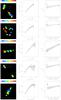 |
Fig. A.1
Left: examples of simulated RM images for the sources A401A, A401B, A2142, A2065, OPHIB. The simulated images have the same colour scale and resolution of the observed RM images. They have been obtained by simulating a RM power spectrum with a spectral index n = 11 / 3 and a minimum scale of the RM fluctuations Λmin = 5 kpc. The maximum scale of the RM fluctuations is Λmax = 205 kpc for A401A and A2142, Λmax = 128 kpc for A401B, Λmax = 15 kpc for OPHIB and A2065. Middle: structure functions of the simulated (grey) and observed (black points) RM images. Right: depolarization plots of the simulations (grey) and observations (black points). The depolarization is defined as DP(ν) = FPOLν / FPOL8465 MHz. |
| Open with DEXTER | |
© ESO, 2010
Current usage metrics show cumulative count of Article Views (full-text article views including HTML views, PDF and ePub downloads, according to the available data) and Abstracts Views on Vision4Press platform.
Data correspond to usage on the plateform after 2015. The current usage metrics is available 48-96 hours after online publication and is updated daily on week days.
Initial download of the metrics may take a while.