| Issue |
A&A
Volume 522, November 2010
|
|
|---|---|---|
| Article Number | A93 | |
| Number of page(s) | 43 | |
| Section | Planets and planetary systems | |
| DOI | https://doi.org/10.1051/0004-6361/200912340 | |
| Published online | 05 November 2010 | |
Short-term variability of a sample of 29 trans-Neptunian objects and Centaurs*,**
Instituto de Astrofísica de Andalucía,
CSIC, Apt 3004,
18080
Granada,
Spain
e-mail: This email address is being protected from spambots. You need JavaScript enabled to view it.
Received:
16
April
2009
Accepted:
5
March
2010
Abstract
Aims. We attempt to increase the number of trans-Neptunian objects (TNOs) whose short-term variability has been studied and compile a high quality database with the least possible biases, which may be used to perform statistical analyses.
Methods. We performed broadband CCD photometric observations using several telescopes (the 1.5 m telescope at Sierra Nevada Observatory, the 2.2 m Calar Alto telescope and the 2.5 m INT on La Palma).
Results. We present the results of 6 years of observations, reduced and analyzed with the same tools in a systematic way. We report completely new data on 15 objects, for 5 objects we present a new analysis of previously published results plus additional data and for 9 objects we present a new analysis of data already published. Lightcurves, possible rotation periods, and photometric amplitudes are reported for all of them. The photometric variability is smaller than previously thought: the mean amplitude of our sample is 0.1 mag and only around 15% of our sample has a larger variability than 0.15 mag. The smaller variability seems to be caused by a bias of previous observations. We find a very weak trend of faster spinning objects towards smaller sizes, which appears to be consistent with the smaller objects being more collisionally evolved, but may also be a specific feature of the Centaurs, the smallest objects in our sample. We also find that the smaller the objects, the larger their amplitude, which is also consistent with the idea that small objects are more collisionally evolved and thus more deformed. Average rotation rates from our work are 7.5 h for the whole sample, 7.6 h for the TNOs alone and 7.3 h for the Centaurs. Maxwellian fits to the period distribution yield similar results.
Key words: Kuiper belt: general / techniques: photometric
Table 1 and Appendix are only available in electronic form at http://www.aanda.org
Table 3 is available in electronic form in the Center of astronomical Data of Strasbourg cdsarc.u-strasbg.fr (130.79.128.5) or via http://cdsweb.u-strasbg.fr/viz-bin/qcat?J/A+A/522/A93 and is available in the link http://www.iaa.es/~ortiz/thirouinetal2010/supportingonlinematerial.pdf
© ESO, 2010
1. Introduction
The rotational properties of the asteroids provide plenty of information about important physical properties, such as density, internal structure, cohesion and shape (e.g., Pravec & Harris 2000; Holsapple 2001, 2004). As for asteroids, the rotational properties of the Kuiper belt Objects (KBOs) provide a wealth of knowledge about the basic physical properties of these icy bodies (e.g. Sheppard & Jewitt 2002; Ortiz et al. 2006; Trilling & Bernstein 2006; Sheppard et al. 2008). In addition, rotational properties provide valuable clues about the primordial distribution of angular momentum, as well as the degree of collisional evolution of the different dynamical groups in the Kuiper belt. Rotational properties can also provide empirical tests of predictions based on models of the collisional evolution of the Kuiper belt (Davis & Farinella 1997; Benavidez & Campo Bagatin 2009).
Studies of short-term photometric variability of Kuiper belt objects allow us to retrieve rotation periods from the photometric periodicities and these studies also provide constraints on shape (or surface heterogeneity) by means of the amplitude of the lightcurves. Therefore, observational programs on time series CCD photometry are a good tool for studing the Kuiper belt. Unfortunately, most KBOs are faint and CCD photometry programs are time expensive and require medium to large telescopes. For this reason and in contrast to the case for asteroids, the sample of KBOs for which short-term variability has been studied is not large and more importantly, the sample of objects with known rotation periods is severely biased toward large photometric amplitudes, the reason being that the large amplitude objects produce lightcurves that are much easier to observe and from which a rotation period can be unequivocally obtained. Very long rotation periods are also difficult to determine and scientists rarely publish null results or failed attempts to derive lightcurves, which causes a bias in the literature. In other words, the scientific literature in the Kuiper belt field consists mostly of high amplitude lightcurves, which are not truly representative of the rotation properties of the whole Kuiper belt population.
Other biases are present in the literature, such as an overabundance of large objects because larger bodies are usually brighter and easier to observe. One can try to avoid this bias by studying Centaur objects, which are not TNOs because they are not farther away than Neptune but are widely accepted to originate in the Kuiper belt; they are thus KBOs that recently came to the inner solar system vicinity, with “recently” meaning time frames of several mega-years, the typical lifetime of Centaurs (Tiscareno & Malhotra 2003). The currently known Centaurs are smaller than TNOs with the same brightness. Therefore, targeting Centaurs provides information about small size objects of the Kuiper belt that would otherwise be too faint for telescopic studies.
Based on the aforementionned ideas we initiated a programme to photometrically monitor as many KBOs as possible, trying to build a reasonably good sample in terms of number of objects observed and also in terms of the amplitude biases. Thus, we published even dubious rotation periods of low-amplitude lightcurve objects rather than omitting them. In their review of asteroid rotation rates, Binzel et al. (1989) emphasized that excluding poor reliability objects gives more weight to asteroids with large amplitudes and short periods, introducing a significant bias.
We present new results from our survey and a reanalysis of several bodies for which we had already published results. We reanalyzed the data for these bodies either because we had acquired more data or because we had developed superior analysis tools that resulted in what we consider an improvement. All the objects presented here were analyzed with the same tools and software and therefore represent a homogeneous data set. The work presented here summarizes a considerable effort in which more than 5000 images were reduced and analyzed.
This paper is divided into 6 sections. Section 2 describes the observations and the data sets. Section 3 describes our software reduction tools and the methods used to derive e.g., periodicities, rotation periods and photometric range. Section 4 deals with the main results obtained for each object and Sect. 5 discusses the results altogether. Finally, our findings are summarized in Sect. 6.
2. Observations
As already mentioned, our group at the Instituto de Astrofísica de Andalucía (IAA, CSIC) started a vast program on lightcurves of the KBOs in 2001. Observations were carried out from the 1.5 m telescope at Sierra Nevada Observatory (OSN – Granada, Spain), from the 2.2 m CAHA telescope at Calar Alto Observatory (Almeria, Spain), and from the 2.5 m Isaac Newton Telescope (INT) at El Roque de Los Muchachos (La Palma, Spain).
The typical seeing during the observations at OSN ranged from 1.0′′ to 2.0′′, with a median seeing around 1.4′′. The observations reported here were carried out by means of a 2k × 2k CCD with a total field of view (FOV) of 7.8′ × 7.8′. We used a 2 × 2 binning mode, which changes the image scale to 0.46′′/pixel. This scale was sufficient to ensure accurate point spread function sampling even in the best seeing cases.
At Calar Alto, the median seeing of the observations was around 0.9′′. For our observations, we used the Calar Alto Faint Object Spectrograph (CAFOS). This instrument is equipped with a 2048 × 2048 pixel CCD. Image scale is 0.53′′/pixel, which is good enough to achieve good sampling for most cases, although for the highest quality seeing some images were slightly undersampled.
At INT, the median seeing was around 1′′. Our observations were obtained with the Wide Field Camera (WFC) instrument. This camera consists of 4 thinned EEV 2154 × 4200 CCDs. Image scale is 0.33′′/pixel, which guarantees good sampling even at the best seeing moments.
Exposure time had to be chosen by considering two main factors. On the one hand, it had to be long enough to achieve a signal to noise ratio (S/N) sufficient to study the observed object. On the other hand, it had to be short enough to avoid elongated images of the target (if the telescope was tracked at sidereal speed) or elongated field stars (if the telescope was tracked at the KBO speed). We always chose to track the telescope at sidereal speed. Our observations concerned, basically, two kinds of objects: TNOs and Centaurs. Drift rate of TNOs is typically low, ~2′′/h, so an exposure time of around ~300 to ~600 s was used.The drift rate of Centaurs is higher than that of TNOs, typically being ~10′′/h. For Centaurs observations, we typically used an exposure time of ~200 s.
Observations were performed either unfiltered or using the Johnson Cousins R filter to maximize the S/N. Among the observations presented in this work, the majority were carried out without filter, while the R filter was used for: 1999 TZ1, Haumea (2003 EL61), Makemake (2005 FY9), Orcus (2004 DW) and Varuna (2000 WR106) and for INT observations. Since the goal of our studies is short term variability, we require relative photometry, not absolute photometry. Therefore, the use of unfiltered images is not a concern for our work. Important geometric data of the observed objects at the dates of observations analyzed here are summarized in Table 1.
Our sample of objects was selected according to the their brightnesses. Very faint objects cannot be observed with a 1.5 m or a 2 m telescope with the needed S/N, thus we restricted our target list to objects brighter than 21 mag in V as predicted magnitudes for the dates of our observing runs according to the minor planet center (MPC) ephemerides generator.
3. Data reduction
During each observing night, a series of bias and flat fields were in general obtained to correct the images. We thus created a median bias and a median flatfield for each day of observation. Care was taken not to use bias or flat field frames that might be affected by observational or acquisition problems. The median flatfields were assembled from twilight dithered images and the results were inspected for possible residuals from very bright saturated stars. The flatfield exposure times were always long enough to ensure that no shutter effect was present so that a gradient or an artifact of some sort could be present in the corrected images. Each target image was bias subtracted and flatfielded using the median bias and median flatfield of the observation day but if daily information about the bias and flat field was not available, we used the median bias and median flat field of a former or subsequent day. No cosmic ray removal algorithms were used and we rejected the images in which a cosmic ray hit or a star was too close to the object.
Relative photometry using as many as 25 field stars was carried out by means of Daophot routines (Stetson 1987). The typical error bars of the individual time integrations were ~0.01 mag for the brightest targets, and 0.06 mag for the faintest objects (in the poorest observing conditions). Care was taken not to introduce spurious results due to faint background stars or galaxies in the aperture. If observations were adversely affected by cosmic-ray hits within the flux aperture, we did not include them in our results.
We used a common reduction software for the photometry data reduction of all the images, but since they came from three different observatories, some parameters of the software were specific for each data set. Those parameters were related to the aperture size, which ranged from 6 to 24 pixels.
The choice of the aperture diameter is important. We had to choose an aperture as small as possible to obtain the highest signal to noise ratio but large enough to include most of the flux. We typically used an aperture radius of the same order as the full width at half maximum (FWHM) of the seeing. We carried out the aperture photometry with several aperture radii values around the FWHM. We also used an adaptable aperture radius, which was different for each image and resulted from the fit of a Moffat star profile to several stars in the field; this allowed us to adapt to the varying seeing during the night. For all apertures used, we chose the results that gave the lowest scatter in the photometry of both the target and of stars with similar brightness as our target. Several sets of reference stars were used to obtain the relative photometry of all the targets, and only the set that gave the lowest scatter was used. In many cases, several stars had to be rejected from the analysis because they exhibited some variability. The final photometry of our targets was computed by taking the median of all the lightcurves obtained with respect to each reference star. By applying this technique, spurious results were eliminated and the dispersion of the photometry improves.
During an observational campaign, we tried to keep the same field and therefore the same reference stars. In some cases, owing to the drift of the observed object, the field changed completely or partially. If the field changed completely, we used different reference stars for two or three subsets of nights in the entire run. If the field changed partially, we tried to keep the greatest number of reference stars in common during the whole campaign. This number varied from 6 to 25. We generated TIFF images within which all the reference stars were marked for each observation night.
When we combined several observing runs, we had to normalize the photometry data to its average because we did not have absolute photometry that would allow us to link one run with the other; in several instances, we did experiment with trying to link several runs by using absolute photometry, and the errors involved were generally much larger than what we can achieve by normalizing the photometry to the mean or median value. Furthermore, the small jumps in the photometry caused by the inevitable absolute photometry offsets cause spurious frequencies in the periodogram analysis. This is especially true for very low variability objects, which are numerous. By normalizing the means of several runs, we assume that a similar number of data points are in the upper part and lower part of the curves. This may not be true if the runs are only two or three nights long, but this is not usually the case. We emphasize that we normalized the mean of each run not the mean of each night.
The final time series photometry of each target was inspected for periodicities by means of the Lomb technique (Lomb 1976) as implemented in Press et al. (1992), but we also verified the results by using several other time series analysis techniques (such as PDM), the Harris et al. (1989) method and the CLEAN technique (Foster 1995). As mentioned before, the reference stars were also inspected for short-term variability. We can thus be confident that no error has been introduced by the choice of reference stars. To measure the amplitudes of the short-term variability, we performed Fourier fits to the data to determine the peak to valley amplitudes (full amplitudes).
As mentioned in Sect. 2, we generally acquired our observations without a filter. Using no filter may be a problem in some cases depending on sky conditions and CCD types. Many CCDs have strong fringing effects caused by near-infrared interference and mainly related to e.g., their pixel size and thinning. But this was not the case for our observations. By obtaining unfiltered images, we reached deeper magnitudes with sufficient signal to noise. We used an R filter when we anticipated that using no filter could be a problem.
In some cases, we combined data obtained without a filter with data obtained with the R filter, for example for 2005 RN43 or 2005 RR43. We assumed that only the lightcurve amplitude is affected when one observes in a different filter, but the rotation period would be the same. Besides, our unfiltered observations are close to R because the CCD sensitivity is usually reaches a maximum at red wavelengths. Thus, we expect this effect to be small, but might alter the periodogram to some degreee.
Even though absolute photometry was not the goal of the observations, we computed approximate magnitudes for a few images per object per observing run. To obtain approximate R magnitudes, we used USNO-B1 stars in the field of view as photometric references. Since the USNO-B1 magnitudes are not standard BVRI magnitudes and because we also did not use BVRI filters, we derived very approximate magnitudes, with a typical uncertainty of 0.4 mag.
The time series photometry of all the objects is provided as Table 3 in the “Center of astronomical Data of Strasbourg” (CDS) and on the link: “www.iaa.es/~ortiz/thirouinetal2010/supportingonlinematerial.pdf”. We have highlighted in bold face the times corresponding to the images that we used to obtain an R magnitude calibration. The remaining R magnitudes in the table were obtained by using the relative magnitude information. In Table 3, we also present are geometric data such as geocentric and heliocentric distance and phase angle. The R magnitudes that the TNOs would have if they were at 1 AU from the Earth and the Sun (mR(1, 1)) are also shown. No phase corrections were applied.
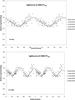 |
Fig. 1 Rotational phase curve for 2003 FY128 obtained by using a spin period of 8.54 h (upper plot) and a spin period of 17.08 h (lower plot). The dash line is a Fourier series fit of the photometric data. Different symbols correspond to different dates. |
4. Photometric results
We present our results in terms of the following classification of KBOs, which are based on dynamical criteria: (i) classical group representing objects under the influence of Neptune and away from the main mean motion resonances; (ii) resonant objects which are in mean motion resonances with Neptune; (iii) scattered disk objects (SDOs) which have a high orbital eccentricity and have had a close encounter with Neptune in the past that sent them to their present position; and (iv) centaurs considered to be similar to TNOs but to reside between Jupiter’s and Neptune’s orbits, after having experienced a close encounter with Neptune. We used the minor planet center lists to classify all these bodies.
The lightcurves and Lomb periodograms for all objects are provided as online material (Fig. A.1 to Fig. A.59). We only present an example of lightcurve in Fig. 1.
4.1. Classical objects
(120132) 2003 FY128 is a classical object observed on 09, 10, 11, 12 February 2005 and 09 March 2005 at the OSN telescope. The Lomb periodogram (Fig. A.1) for our data contains an important peak (confidence level >99%) at 8.54 h (2.81 cycles/day), which is a single peaked periodicity. A double peaked periodicity of 17.08 h might be more appropriate because the fit to a Fourier series shows minima and maxima of different values, but neither PDM nor the Harris method, which are less sensitive to the exact shape of the lightcurve, proposed a periodicity 17.08 h (Fig. 1 and Fig. A.2). The amplitude is 0.15 ± 0.01 mag. A second high peak in the periodogram of a lower spectral power is located at 1.76 cycles/day, which appears to be an alias.
Sheppard (2007) observed this object in the R band on 09, 10 March 2005 at the Dupont 2.5 m telescope in Las Campanas in Chile. They presented a very flat lightcurve based on 17 data points. They noted that 2003 FY128 has no significant short-term variability. A small amplitude <0.08 mag was suggested. Dotto et al. (2008) observed this object on 18, 19 April 2007 at the 3.0 m New Technology Telescope (NTT) at the European Southern Observatory at La Silla (Chile). Their photometry appears to be inconsistent with some slight short-term variability. They presented more than 13 h of observations, in R band but could not determine a rotational period. Their own evaluation suggests a short-term variability longer than 7 h.
In conclusion, we present the first lightcurve of this object. A period longer than 7 h proposed by Dotto et al. (2008) is consistent with our results.
(174567) 2003 MW12 is a classical object. This body was observed on 28 May 2006, on 05, 06, 07, 10, 23, 24 June 2006 and on 12, 13, 14, 26, 27 April 2008 at the OSN telescope. We present two possible lightcurves (Fig. A.3), one based on a single peak periodicity of 5.9 h (4.07 cycles/day) and another single peaked one of 7.87 h (3.04 cycles/day), which appears to be an alias. The Lomb periodogram (Fig. A.4) suggests a periodicity of 5.9 h, but the Harris, PDM and CLEAN techniques infer a 7.87 h period. The amplitude of the curve is 0.06 ± 0.01 mag. From visual inspection, the best-fit lightcurve is obtained for a period of 5.9 h because the alternative fits exhibit more scatter. To our knowledge, there is no published photometry of this object to compare with. We present the first lightcurve of 2003 MW12 and propose a periodicity of 5.9 h or 7.87 h for this object.
(120178) 2003 OP32 is a classical object observed on 05, 06, 07, 08, 10 March 2005, on 03, 04, 05 October 2005 and on 15, 16, 17 September 2007 at the OSN telescope. We propose a 0.13 ± 0.01 mag amplitude lightcurve with a short-term variability of 4.05 h (5.93 cycles/day) (Fig. A.5). A double peaked periodicity of 8.1 h is neither supported nor excluded by the data. The Lomb periodogram (Fig. A.6) shows another high peak at 6.97 cycles/day and a second peak smaller than the first one (but with a high confidence detection level) at 4.89 cycles/day. They both appear to be aliases of the main periodicity. All techniques used confirm a periodic signature at 4.05 h.
We found one bibliographic reference for this target: Rabinowitz et al. (2008) presented the results of R band observations carried out in 2006 July 17–2006 November 23 at the 1.3 m SMARTS telescope. Seventy-eight sparse sampled data points formed a 4.845 h lightcurve with an amplitude of 0.26 mag.
Our results appear to be of much higher photometric precision than those of Rabinowitz et al. (2008) as our lightcurve has a far smaller scatter and is based on 147 data points. The large 0.26 mag amplitude is rejected by our data, which were optimized for period determination rather than for phase coefficient determination (the primary goal of the sparse sampled observations by Rabinowitz et al. 2008).
(120347) 2004 SB60 is a classical binary object. The magnitude difference between this object and its satellite is 2.3 (Noll et al. 2006). This object was observed on 05, 06, 07, 10 August 2005 and on 03, 04, 06, 07 August 2008 at the OSN telescope. We present (Fig. A.7) two lightcurves: a single peaked periodicity of 6.09 h (3.94 cycles/day) or 8.1 h (2.96 cycles/day). An amplitude of 0.03 ± 0.01 mag is seen in both cases. Double peaked lightcurves at 12.18 h or 16.02 h period do not appear to be more distinctive. PDM, CLEAN and Lomb techniques (Fig. A.8) favor a periodicity of 6.09 h, but the Harris method detects a period of about 8.1 h.
To our knowledge, there is no bibliographic source on 2004 SB60 rotational variability. We present the first lightcurve of this body. As in the case of 2003 MW12, we cannot clearly favor a rotational period of either 6.09 h or 8.1 h. For very low amplitude objects, we know that very small night to night offsets in the photometry can transfer a lot of power from the main peak to a 24 h-alias and viceversa. Therefore, even though 6.09 h is the preferred result, 8.1 h is also quite possible and that could be true for other aliases.
2005 CB79 is a classical object. This object was observed on 06, 07 January 2008 at the Calar Alto telescope, on 01, 04 May 2008 and 26 December 2008 at the OSN telescope. A single peaked periodicity of 6.76 h (3.55 cycles/day) is indicated by the Lomb periodogram (Fig. A.9). The lightcurve has an amplitude of 0.13 mag (Fig. A.10). A double peaked periodicity of 13.52 h is not preferred by any of the time series analysis methods. Apparent aliases are at 2.55 cycles/day and at 4.55 cycles/day. All the techniques measure the same periods.
(145452) 2005 RN43 is a classical body observed on 22 October 2006 at the INT and on 14, 16, 17, 19 September 2007 and 03, 04, 05, 07, 08 August 2008 at the OSN telescope. The Lomb periodogram (Fig. A.11) exhibits a high peak with a >99% confidence level at 5.62 h (4.28 cycles/day) and a second peak with a lower confidence level at 7.32 h (3.27 cycles/day). The lightcurve has an amplitude of 0.04 ± 0.01 mag (Fig. A.12). PDM, CLEAN and the Harris techniques confirm that the peak is located at 7.32 h. We cannot conclusively favor one period over the other for similar reasons as for 2004 SB60, but 7.32 h appears the most likely.
(145453) 2005 RR43 is a classical object observed on 22, 23, 26 October 2006 at INT, on 15, 16, 17, 18 December 2006, on 11, 12, 13, 14, 15, 16 January 2007 at the Calar Alto telescope and on 14, 15, 17 September 2007 at the OSN telescope. The Lomb periodogram (Fig. A.13) exhibits several peaks. We note a significant peak located at 7.87 h (3.05 cycles/day) and a second peak of a lower significance level at 6.35 h (3.78 cycles/day). PDM identifies the same peaks at the same values and a third peak at 4.1 cycles/day. We present a lightcurve with a single peak periodicity of 7.87 h (3.05 cycles/day) (Fig. A.14). A double peaked lightcurve at 15.74 h does not appear more likely than the 7.87 h period. The amplitude of the periodic signal is 0.06 ± 0.01 mag.
(50000) Quaoar (formerly 2002 LM60) is a binary classical object. The magnitude difference between Quaoar and its satellite is 5.6 ± 0.2 mag (Brown & Suer 2007). Quaoar was observed on 21, 22, 23 May 2003, on 17, 18, 19, 20, 21, 22 June 2003 at the OSN telescope. The Lomb periodogram (Fig. A.15) for this object shows one peak with a high spectral power corresponding to a periodicity at 8.84 h (2.72 cycles/day), but a double peaked lightcurve at 17.68 h provides a more probable fit because there appear to be two maxima of different height. Both, the PDM and CLEAN techniques confirmed the single peaked period with a high spectral power but the Harris method suggests the double peaked periodicity. The lightcurves are shown in Fig. A.16 both of which have an amplitude of 0.15 ± 0.04 mag.
Our data were used in Ortiz et al. (2003b), who inferred a 17.67883 h double peaked periodicity with a confidence level above 99.9% and an amplitude of 0.133 mag. This object was later observed by Rabinowitz et al. (2007). They presented on 166 R band observations carried out using the 1.3 m telescope of the small and moderate aperture research telescope system (SMARTS). Rabinowitz et al. (2007) suggested a 8.84 h single peaked rotational lightcurve with an amplitude of 0.18 mag, which is consistent with our results.
Lin et al. (2007) presented R band results based on the analysis of 57 images acquired in 03, 04 June 2003 and using the Lulin one-meter Telescope (LOT). They proposed a 9.42 h single peaked rotational lightcurve with a confidence level higher than 99.9% and a ~0.3 mag amplitude. Such a high amplitude is inconsistent with both our results and those of Rabinowitz et al. (2007), which were obtained using larger telescopes and data sets.
In conclusion, we propose a 17.68 h double peaked periodicity or a 8.84 h single peaked periodicity.
(20000) Varuna (formerly 2000 WR106) is a classical object. Varuna was observed on 05, 07, 31 January 2005 and on 01, 09, 10 February 2005 at the OSN telescope. The Lomb periodogram (Fig. A.17) for this object shows a very clear peak with a high spectral power corresponding to a periodicity of 3.1709 h (7.57 cycles/day), but a double peaked lightcurve for a period twice that value has smaller scatter. PDM confirms the 6.3418 h period. The lightcurve is depicted in Fig. A.18 and shows an amplitude of 0.43 ± 0.01 mag.
Ortiz et al. (2003a) presented results of observations at the OSN 1.5 m telescope on 08, 09 February 2002. In that work, a lightcurve with an amplitude of 0.41 mag and a 6.3436 h double peaked rotational (3.1718 h single peak) was proposed. Varuna was also observed by Farnham (2001), who presented results of observations carried out on January, March and September 2001. They proposed a 6.34 h double peaked rotational lightcurve with an amplitude of 0.50mag. Sheppard & Jewitt (2002) used R-observations made on 17-18-19-20 February and April 2001 at the 2.2 m University of Hawaii telescope. They suggested a 6.34 h double peaked rotational lightcurve with a 0.42 mag amplitude. Belskaya et al. (2006) presented R-observations carried out on November, December 2004 and on January, February 2005. Observations were made at 1.5 m OSN telescope and at the bulgarian 2 m Ritchey-Chretien-Coude telescope. They obtained a 6.34358 h double peaked rotational lightcurve with an amplitude of 0.42 mag for phase angles larger than 0.8° and 0.47 mag near opposition. In Belskaya et al. (2006), it was shown that the lightcurve amplitude of Varuna increases at small phase angles.
Rabinowitz et al. (2007) observed Varuna on 30 December 2004 and 17 April 2005. They presented photometric results based on 78 images. They suggested a 6.344 h double peaked rotational lightcurve with an amplitude of 0.49 mag.
Even though most of the works are consistent with a 0.42 mag amplitude lightcurve, the works by Farnham (2001) and Rabinowitz et al. (2007) measured a larger amplitude. However, Farnham (2001) does not quote the uncertainty in his derivation. On the other hand, Rabinowitz et al. (2007) data were not optimized for short-term variability studies. The differences might therefore arise because of the different quality of the data, but since part of the small discrepancies in the amplitude of the lightcurve reported by the various authors could be due to the phase angle variability reported in Belskaya et al. (2006), we recall that the observations of Ortiz et al. (2003a) were taken at phase angles between α = 0.81° and 0.83°, those by Farnham (2001) covering the range α = 0.57°–0.63°, those by Sheppard & Jewitt (2002) being taken at around 1° in February 2001 and around 1.2° in April 2001, those by Belskaya et al. (2006) being taken between α = 0.056° and 0.92° and those by Rabinowitz et al. (2007) covering the range α = 0.06°–1.3°. In conclusion, there is little question that Varuna has a double peaked lightcurve and a 6.34 h rotational period with 0.42 ± 0.01 mag amplitude, outside the opposition surge.
(55565) 2002 AW197 is a classical object observed on 01–02 February 2003 and on 19, 21, 22, 23, 24, 25 January 2004 at the OSN telescope.
The Lomb periodogram (Fig. A.19) of this object contains several peaks with significant confidence levels. The highest peak is located at 8.78 h (2.74 cycles/day). The PDM, CLEAN and Harris techniques favored a rotational period of 8.78 h. The lightcurve of this object (Fig. A.20) has a very small amplitude 0.04 ± 0.01 mag. Thus it is difficult to judge whether a double peaked lightcurve would be better.
Ortiz et al. (2006) published a possible 2002 AW197 lightcurve. They used observations of 29 November 2002, 01, 03, 05, 07, 08 December 2002, 01, 02, 03 February 2003 and 21, 22, 23, 25, 26 January 2004. Ortiz et al. (2006) presented a Lomb periodogram with several high peaks (confidence level >99.9%). The highest peak was located at 8.86 h and was accompanied by two aliases, with lower spectral power than the first peak, at 13.94 h and at 6.94 h. Another peak with high confidence was identified at 15.82 h. Ortiz et al. inferred, a 8.86 h period for a single peaked rotational lightcurve with a reliability code of 2 (reliability code according to the definition given in Lagerkvist et al. 1989).
Sheppard (2007) observed this body in the R band on 23, 24 December 2003 at the University of Hawaii 2.2 m telescope. They presented a very flat lightcurve based on 27 data points. They noted that 2002 AW197 has no significant short-term variability. A small amplitude <0.03 mag was suggested.
In conclusion, 2002 AW197 has a nearly flat lightcurve and we propose a 8.78 h rotation period, although one should keep in mind that for the very low amplitude objects many of the apparent 24 h aliases are also probable.
(55636) 2002 TX300 is a classical object that was observed on 07, 08, 09 August 2003 at the OSN telescope.
The Lomb periodogram (Fig. A.21) identifies a single peak periodicity of 4.08 h (5.88 cycles/day) but PDM and the Harris method determine the true periodicity to be twice that value (8.16 h), with a 0.04 ± 0.01 mag amplitude for the 4.08 h period and 0.08 ± 0.01 mag for the 8.16 h period. Figure A.22 shows the lightcurve for 8.16 h.
Ortiz et al. (2004) presented observations performed on 29, 30 October 2002, on 06, 07, 28, 29, 30 November 2002 and on 02, 03, 04, 06 December 2002. Coordinated observational campaigns were arranged at three different telescopes: the 1.5 m OSN telescope, the 3.6 m Canada-France-Hawaii Telescope (CFHT) and the 2.5 m Nordic Optical Telescope (NOT) at La Palma for the photometric study. Results of this coordinated campaign showed a 7.89 h peaked rotational lightcurve with an amplitude of 0.09 ± 0.08 mag.
Here, we used additional images from two nights that were not available in Ortiz et al. (2004). In Ortiz et al. the two larger aperture telescopes provided a few data that could be used to check whether the 7.89 h was consistent with those observations or not. On the other hand, data from the larger aperture telescopes were scarce and of poorer quality than the data from the 1.5 m OSN telescope. Therefore, we consider 8.16 h to be more probable than 7.89 h.
Sheppard & Jewitt (2003) presented a 8.12 h or a 12.1 h single peaked rotational R band lightcurve with an amplitude of 0.08 ± 0.02 mag.
Thus, our results and those of Sheppard’s are consistent and not far from the Ortiz et al. (2004) results. This implies that a rotation period of 8.14 ± 0.02 h with a photometric range of 0.08 ± 0.02 mag is secure.
(55636) Makemake (formerly 2005 FY9) is a classical object. This object was observed on 07, 08, 10, 12 April 2005, on 27–29 May 2006, on 05, 07, 10 June 2006, on 14–18 December 2006 and on 09–12 March 2007 at the OSN telescope and on 11–16 January 2007 at Calar Alto telescope. This object was extensively observed because it had an extremely low (and challenging) variability. The Lomb periodogram (Fig. A.23) shows two broad maxima containing many sharp spikes. The two maxima correspond to ~7.7 h (~3.1 cycles/day) and its 24-h alias at ~11.5 h (2.1 cycles/day). The period of 7.7 h is slightly more likely in terms of spectral power, but the exact spike at which the lightcurve is more accurately fit is not straightforward to find. We chose 7.64 h and the corresponding lightcurve is shown in Fig. A.24. With fewer data, Ortiz et al. (2007) favored what we understand to be the 24-h alias. As mentioned before, much spectral power is easily transferred from one peak to its 24-h alias in low variability objects, for which 2005 FY9 is the most extreme case that we deal with in this paper. Very slight night to night calibration errors are the reason for the transfer of spectral power. Thus, it is difficult to decide which is the correct period. However, since we have a large number of nights, random night-to-night offsets should cancel on average. Thus, we believe that 7.7 h is more likely than the value that was derived with fewer nights in Ortiz et al. (2007). The amplitude of the lightcurve obtained by means of a sinusoidal fit is 0.015 ± 0.005 mag.
4.2. Resonant objects
(126154) 2001 YH140 was observed on 15, 16, 17, 18, 19 December 2004. This object is in resonance 3:5 with Neptune. The Lomb periodogram (Fig. A.25) and PDM show three peaks of high spectral power located at 13.2 h (1.82 cycles/day), 8.40 h (2.86 cycles/day) and 6.19 h (3.88 cycles/day). The lightcurve for a rotation period of 13.2 h is shown in Fig. A.26. The amplitude of the lightcurve is 0.13 ± 0.05 mag.
Using data from 15–20 December 2004, Ortiz et al. (2006) favored a periodicity of 8.45 h but, presented two aliases located at 6.22 h and at 12.99 h. Sheppard (2007), from R band observations, taken on 19, 21, 23, 24 December 2003 at the University of Hawaii 2.2 m telescope, suggested a double peak periodicity of 13.25 h with an amplitude of 0.21 ± 0.04 mag.
In summary, there is agreement about the rotation period of this body, bearing in mind that 13.20 h is very close to the 12.99 h possible alias reported in Ortiz et al. (2006). However, the amplitude that we report is somewhat different, although consistent within their error bars.
We propose a lightcurve with a single peak periodicity of 13.2 h and an amplitude of 0.13 ± 0.04 mag, which appear to be consistent with the data by Sheppard (2007).
(90482) Orcus (formerly 2004 DW) is a binary object in resonance 2:3 with Neptune. The magnitude difference between this object and its satellite is 2.54 ± 0.01 mag (Brown et al. 2010). Our observations were carried out on 08, 09, 11, and 23 March 2004 and on 22, 23, 25, 26, 27 April 2004 at the OSN telescope. The Lomb periodogram (Fig. A.27) and PDM technique show one peak with a high significance level (>99%) located at 10.47 h (2.29 cycles/day). We propose a lightcurve with this period in Fig. A.28 with an amplitude of 0.04 ± 0.01 mag. All techniques PDM, CLEAN and Harris suggest the same period of 10.47 h.
Ortiz et al. (2006) presented observational results on 08, 09, 10, 11 March 2004 and on 22, 23, 25, 26, 27 April 2004. The work published by Ortiz and the present work used almost the same data but the present work considers data for two more nights. The Lomb periodogram showed three peaks with a high confidence levels (>99.9%) located at 7.09 h, 10.08 h, and 17.43 h. The 7.09 h and 17.43 h periods were probably aliases of the 10.08 h periodicity that appeared most likely. Applying different techniques such as PDM, CLEAN and chi- square minimization, etc., the value 10.08 h was favored with a reliability code of 2 (reliability code according the definition given in Lagerkvist et al. 1989).
Sheppard (2007) observed Orcus on 14, 15, 16 February 2005 and on 09, 10 March 2005 with an R-filter. His results were based on 43 images carried out at the Dupont 2.5 m telescope at Las Campanas in Chile. He did not notice a significant short-term variability. Lightcurves of each observational night suggested a flat lightcurve with an amplitude <0.03 mag.
Rabinowitz et al. (2007) presented photometric results of 143 images carried out on 21 February to 6 July 2004 using the 1.3 m SMARTS telescope. They suggested a 13.19 h single peaked rotational lightcurve with an amplitude of 0.18 mag. This is obviously inconsistent with both Sheppard (2007) and our work, in terms of both period and amplitude.
In conclusion, we present a lightcurve based on 327 images for which we found a periodicity of 10.47 h, similar to Ortiz et al. (2006). Because of the small amount of data from Sheppard (2007), no period was reported. Since the object has a very low amplitude some of the 24 h aliases (at 7.3 h, 5.6 h and 18.54 h) could be the true rotation too.
(555638) 2002 VE95 was observed on 19 January 2004 and on 15, 16, 17, 18 and 19 December 2004 at the OSN telescope. This object is in resonance 2:3 with Neptune. The Lomb periodogram (Fig. A.29) for this object and PDM do not allow us to identify a clear rotational periodicity. We note a high peak at 9.97 h (2.41 cycles/day) and three aliases at 17.32 h (1.39 cycles/day), 6.18 h (3.88 cycles/day) and 4.90 h (4.90 cycles/day). We obtain a lightcurve (Fig. A.30) with a 9.97 h periodicity and an amplitude of 0.05 ± 0.01 mag.
Ortiz et al. (2006) presented observations carried out on 29 November 2001, 03, 04, 08 December 2002 and on 15, 16, 17, 18, 19, 20 December 2004. The Lomb periodogram showed three high peaks with a confidence level >99.9% located at 6.76 h, 7.36 h and 9.47 h. Studying the data with other techniques, such as PDM, a 6.88 h high peak was detected. The CLEAN technique confirmed the peak detected by PDM. Ortiz et al. (2006) did not favor or discard any periodicity. In all cases, the amplitude of the lightcurve was below 0.08 mag.
This object was also observed by Sheppard & Jewitt (2003). They presented results of observations made on the University of Hawaii 2.2 m telescope during one night. They could not determine a periodicity. An amplitude variation of <0.06 mag was detected during their observations.
In conclusion, even though the periodicity that we detect is above the 99% confidence level, the periodicityis probably caused by small instrumental errors that are difficult to evaluate. One should keep in mind that 2002 VE95 has very low amplitude variations and the overall scatter of our data is greater than for other low variability objects that we have studied in more detail. Since Ortiz et al. (2006) did not identify any periodicity and Sheppard & Jewitt (2003) could not determine a period, our derivation is only tentative and more observation data with smaller scatter will be necessary to derive a rotation period completely reliable.
(208996) 2003 AZ84 is a binary object in resonance 2:3 with Neptune. The magnitude difference between this object and its satellite is 5.0 ± 0.3 mag (Brown & Suer 2007). This object was observed on 22, 23, 24, 25 January 2004 and on 14, 15, 16, 17, 18, 19 December 2004 at the OSN telescope. The Lomb periodogram (Fig. A.31) has one peak located at 3.53 cycles/day (6.79 h). In Fig. A.32, we present a 6.79 h single peaked lightcurve with an amplitude of 0.07 ± 0.01 mag. This period is also derived from the PDM analysis and both the CLEAN and Harris methods. Ortiz et al. (2006) presented data acquired on 20, 22, 25, 26 January 2004 and 15, 16, 17, 18, 19, 20 December 2004, the Lomb periodogram of which exhibited several peaks of a very high confidence level. The highest peak was located at 5.28 h and presented two aliases of similar spectral power at 4.32 h and at 6.76 h.
Sheppard & Jewitt (2003) studied three observation nights: 23, 24, 25 February 2003 using the University of Hawaii 2.2 m telescope. They presented a 6.72 h single peaked rotational lightcurve with an amplitude of 0.14 mag.
Thus, we conclude that a rotation period is 6.75 ± 0.04 h (a double peaked lightcurve at 13.5 h is apparently no more likely than 6.75 h).
(84922) 2003 VS2 was observed on 22, 26, 28 December 2003, on 04, 19, 20, 21, 22 January 2004 at the OSN telescope. This object is in resonance 2:3 with Neptune. The Lomb periodogram (Fig. A.33) and PDM technique show a clear main peak with a high confidence level (>99%). We propose a short-term variability of 3.71 h (6.47 cycles/day), but the double peaked version (7.42 h) is more appropriate and corresponds to a clearer lightcurve with the two maxima and two minima of different values (Fig. A.34). An amplitude of 0.21 ± 0.01 mag is derived from our data.
Ortiz et al. (2006) presented data reduction of observations carried out on 22, 23, 26, 28, 29 December 2003 and 21, 22 January 2004. The Lomb periodogram showed two peaks with a high significance level at 3.71 h and 4.39 h. The second value was an alias of the first value. The amplitude was estimated as 0.23 mag.
Our results are also consistent with Sheppard (2007), who presented a study of observations made with the University of Hawaii 2.2 m telescope. Observations were carried out on 19-21-23-24 December 2003 with an R-filter. They proposed a lightcurve with a double peak periodicity of 7.41 h with an amplitude of 0.21 mag.
In conclusion, there is clear evidence that a 7.42 h periodicity of 2003 VS2 is its true rotation period. The lightcurve presents an amplitude of 0.21 ± 0.01 mag.
(144897) 2004 UX10 was observed on 14, 17 September 2007 and on 30 November 2007 at the OSN telescope. This object is in resonance 2:3 with Neptune. The Lomb periodogram (Fig. A.35) shows three peaks with a high confidence level (>99%) at 4.23 cycles/day (5.68 h), at 3.88 cycles/day, and at 4.58 cycles/day. The highest peak is 4.23 cycles/day and the other values resemble aliases. However, all of them have very similar spectral power. PDM determines a periodicity of 5.30 h. This value is consistent with the Lomb one. We propose (Fig. A.36) a lightcurve with a short-term variability of 5.68 h (4.23 cycles/day). A double peaked periodicity of 11.36 h does not give produce a closer fitting lightcurve and the amplitude of 0.08 ± 0.01 mag is indicated by the fits.
To our knowledge, we present the first photometric study of 2004 UX10 so there is no literature source with to compare our results which. From our results, a periodicity of 5.68 h is possible, but because of the presence of aliases and the low amount of data relative to those for other objects, it is safer to conclude that the rotation period is between 5 and 7 h. More observations would be needed to derive a more precise period for this object.
(136108) Haumea (formerly 2003 EL61) is considered as a resonant object by Ragozzine & Brown (2007) at the 7:12 resonance with Neptune, although it was listed as belonging to the classical type by the Minor Planet Center for quite some time. The magnitude differences between Haumea and its satellites Hi’iaka and Namaka, are 2.98 ± 0.03 mag and 4.6 mag (respectively) (Lacerda et al. 2008). We present results of R band observations on 12, 13, 14, 15, 16, 17 January 2007 at the 2.2 m Calar Alto telescope. We obtained a double peaked lightcurve with a periodicity of 3.9153 h (single peak periodicity of 1.9577 h (12.24 cycles/day) indicated by the Lomb periodogram (Fig. A.37)), but both the PDM and Harris methods found the double peaked periodicity. The amplitude of our lightcurve is 0.28 ± 0.02 mag (Fig. A.38).
Rabinowitz et al. (2006) presented R-observations acquired on 25 January–26 July 2005 using the 1.3 m SMARTS telescope. They used additional observations on 10–12 April 2005 at the 5.1 m Hale telescope at Palomar Observatory and on 4 May 2005 at the 0.8 m telescope at Tenagra Observatory. They derived a 3.9154 h double peaked rotational lightcurve with an amplitude of 0.28 mag from their data.
Lacerda et al. (2008) used observations carried out on 11, 13, 15 June 2007 and on 07, 08, 22, 24 July 2007 at the 2.2 m University of Hawaii telescope. Observations wereperformed using the R, B, and J filter. They obtained a 3.9155 h double peaked rotational lightcurve with an amplitude of 0.29 mag.
Thus, there is little doubt that 3.9154 ± 0.0001 h is the correct rotation period, as there is wide agreement on this from three independent data sets. The same is true for the amplitude of the variability.
4.3. Scattered disk objects (SDOs)
(145451) 2005 RM43 was observed on 13, 14 October 2006, 15, 17, 18 December 2006 at the OSN telescope and on 11, 12, 13, 14, 15 January 2007 at the Calar Alto telescope. The Lomb periodogram (Fig. A.39) exhibits a very high peak at 3.58 cycles/day (6.71 h) and two aliases of this peak at 2.58 and 3.80 cycles/day. The lightcurve (Fig. A.40) appears to have an amplitude of 0.04 ± 0.01 mag. PDM confirms the first peak and shows these two other peaks with a lower confidence level. We are therefore able to confirm a periodic single peaked lightcurve of 6.71 h (3.58 cycles/day) and a double peaked periodicity of 13.42 h. All other period finding techniques imply a periodicity of around 6.7 h. There is no bibliographic reference with which to compare our results.
(42355) Typhon (formerly 2002 CR46) is a binary object. The magnitude difference between this object and its satellite is 1.30 ± 0.06 mag (Grundy et al. 2008). Typhon was observed on 28 January 2003 and on 02, 04, 06, 09 March 2003 at the OSN telescope. The Lomb periodogram (Fig. A.41) shows several peaks, but one of them has a much higher spectral power. Thus, we present a lightcurve corresponding to this periodicity in Fig. A.42 that has a 9.67 h (2.48 cycles/day) single peak period, a very small amplitude 0.07 ± 0.01 mag. 24 h-aliases are also present. All techniquesinfer consider results.
Ortiz et al. (2003a) presented observations carried out on 08-10 March 2002. The Lomb periodogram showed two peaks, with a confidence level below 50%, located at 3.66 h and 4.35 h. Both values were aliases. Because of a low significance level, no period was favored. The amplitude was reported to be <0.15 mag.
Sheppard & Jewitt (2003) observed Typhon during 4 nights using the University of Hawaii 2.2 m telescope, but their study could not estimate a periodicity. They presented a flat lightcurve with an amplitude <0.05 mag, which is consistent with our findings.
In conclusion, Typhon presents a nearly flat lightcurve, according to our result and published articles. The period proposed in the present work is tentative as we know that low variability objects are easily affected by small night-to-night instrumental/observation changes that can artificially accentuate the power of some spurious frequencies.
(15874) 1996 TL66 was observed on 15, 16, 17, 18 December 2004 at the OSN telescope. The Lomb periodogram (Fig. A.43) shows several peaks all of equally low confidence. We cannot reliably determine a periodicity. We are only able to identify the peak with the highest spectral power at 8.04 h (2.99 cycles/day) and two aliases located at 12 h and 6 h. The lightcurve presented in Fig. A.44 is a single peak periodicity of 12 h with an amplitude of 0.07 ± 0.02 mag. The CLEAN and the Harris analysis suggest a period of 5.1 h and PDM propose 10.2 h.
Using data obtained on 14–19 December 2004, Ortiz et al. (2006) presented a 12.1 h single peaked rotational lightcurve with a <0.12 mag amplitude. But according to the reliability code assigned to this value by Ortiz et al. (2006); code defined in Lagerkvist et al. 1989) this period is clearly uncertain.
Luu & Jewitt (1998) used the 6.5 m Multiple Mirror Telescope (MMT) on Mount Hopkins, Arizona to observed this object in the R band. Observations were made during one night (over 6 h) on 15 October 1996. They noted an amplitude <0.06 mag but they could not determine a periodicity.
This object was also observed by Romanishin & Tegler (1999) with the 2.3 m telescope on Kitt Peak, Arizona. Observations were made between the 2nd and the 9th of October 1997 in V band. Results were based on only 25 images. They could not identify a short-term periodicity, but they noted an amplitude <0.06 mag.
In conclusion, the periodicity of this object is uncertain, there being indications of 12 h and its diurnal aliases. There are also indications of 10.2 h and even 5.1 h. With more observations, a more reliable period might be secured.
4.4. Centaurs
(52872) Okyrhoe (formerly 1998 SG35) was observed on 05, 06, 07, 08, 10, 11, 12, 13, 14, 15 December 2006 at the OSN telescope. The Lomb periodogram (Fig. A.45) suggests a single peaked periodicity of 4.86 h (4.94 cycles/day) or 6.08 h (3.95 cycles/day) and double peaked periodicities of 9.72 h or 12.16 h are also possible, but there is no clear evidence that they are any better. Lightcurves present the 4.86 h and the 6.08 h periods (Fig. A.46). An amplitude of 0.07 ± 0.01 mag is suggested from the fits. The CLEAN method suggested a 6.08 h period, whereas the Harris method and PDM imply a 4.86 h. This is not surprising because both peaks in the periodogram have almost the same power.
Bauer et al. (2003) observed Okyrhoe at the University of Hawaii 2.2 m telescope. Observations were performed during 3 consecutive nights from 22 to 24 September 1999, in R band. Their result was a 16.6 h double peaked rotational lightcurve with an amplitude of 0.2 mag. However, such a high amplitude is ruled out by our data so we suggest that some kind of observational, instrumental, or reduction problem affected their photometry.
In conclusion, 4.86 h and 6.08 h appear as possible values.
(145486) 2005 UJ438 was observed on 11, 12, 13, 15, 16 January 2007 and 06, 07 January 2008 at the Calar Alto telescope and on 26 December 2008 at the OSN telescope. The Lomb periodogram (Fig. A.47) shows several peaks with high spectral power at 4.16 h (5.77 cycles/day). This is the highest peak but there are important diurnal aliases. We propose a single peaked periodicity of 4.16 h (5.77 cycles/day) with an amplitude of 0.13 ± 0.01 mag (Fig. A.48). CLEAN, Harris, and PDM all determine a 4.18 h rotational period.
There is no literature reference on photometric results for this body that we are aware of. Thus we cannot compare our results with others and our preliminary conclusion is that 4.18 h seems a reasonable value with the caveats that the apparent 24-h aliases can be the true periodicity.
2002 KY 14 = 2007 UL126 was observed on 01, 02, 03, 04, 05 August 2008 at the OSN telescope. The Lomb periodogram (Fig. A.49) and PDM technique show two peaks with a high spectral power located at 3.56 h (6.74 cycles/day) and at 4.2 h (5.71 cycles/day). In both cases, the lightcurve (Figs. A.50 and A.51) has an amplitude of 0.13 ± 0.01 mag. CLEAN, PDM, and Harris suggest a 4.2 h rotational period. Thus we adopt this asour most likely estimate of the rotation period. Double peaked versions of the two mentioned periodicities do look slightly more probable but there is no quantitative evidence to suppor this impression. In conclusion, 3.56 h and 4.2 h are possible rotation periods.
(55567) Amycus (formerly 2002 GB10) is a binary TNO observed on 08, 09 March 2003 at the OSN telescope. The Lomb periodogram Fig. A.5) shows two peaks with a high spectral power at 2.46 and 1.48 cycles/day (9.76 h and 16.21 h respectively). The other period finding methods suggest periods of between 9.7 h and 10.1 h. These peaks have a similar spectral power, but 9.76 h is preferred. We propose a lightcurve corresponding to this period. A single peak lightcurve of 9.76 h (2.46 cycles/day) is presented in Fig. A.53. The amplitude of the variability is 0.16 ± 0.01 mag.
As far as we know, there is no bibliographic reference for the time series analysis of Amycus that we can use to compare with and improve our study. In conclusion, we can estimate a clear periodicity around ~10 h. More observations shouldl permit us to determine a more precise rotational period.
(120061) 2003 CO1 is a binary object observed on 19, 21, 22, 23, 24, 25 January 2004 and on 19, 23, 25, 26, 27 April 2004 at the OSN telescope. The Lomb periodogram (Fig. A.54) exhibits several peaks. We propose a lightcurve with a single peak periodicity of 4.51 h (5.31 cycles/day) and an amplitude of 0.07 ± 0.01 mag (Fig. A.55). Apparent aliases are at 4.3 cycles/day and 6.3 cycles/day. All methods confirm that the 4.51 h period is the most likely choice.
The Lomb periodogram in Ortiz et al. (2006) proposed several possibilities of a 3.53 h, 4.13 h, 4.99 h or 6.30 h rotational period. Ortiz et al. (2006) favored a 4.99 h single peaked rotational lightcurve. In all cases, the amplitude was 0.1 mag.
In conclusion, with the same observational data, our result and Ortiz et al. (2006) result proposed somewhat different periods but once aliases are taken into account, the closest agreement seems to be around the 5 h range.
(136204) 2003 WL7 was observed on 05, 06, 07, 08, 10, 11, 13, 14 December 2007 at the OSN telescope. The Lomb periodogram (Fig. A.56), PDM, CLEAN, and the Harris techniques suggest one main periodicity located at 8.24 h (2.92 cycles/day). We propose a lightcurve based on that period (Fig. A.57). The amplitude is 0.05 ± 0.01 mag. A double peaked periodicity of 16.48 h is not preferred by any criteria so we propose 8.24 h period as our most robust estimate.
There is no bibliographic reference of photometric results for 2003 WL7 with which we can compare with. Based on 303 images, our result appaears to be robust enough and 8.24 h seems a secure value, but the low amplitude of the variations raises some concerns that one of the diurnal aliases might be more appropriate.
(12929) 1999 TZ1 was initially classified as a Centaur and is still listed as such in the Minor Planet Center. Moullet et al. (2008) clearly demonstrated that 1999 TZ1 is a Jovian Trojan. We should have chosen not to include this object in our study, but since the object is still listed as a Centaur and because Trojans are also linked to TNOs according to one of the dynamical models of the Kuiper belt formation and evolution (Morbidelli et al. 2005), its presence should not contaminate our sample too much. In this work, we present data reduction of observations carried out on 23–25 February 2007, on 09, 10, 11, 12 March 2007 at the OSN telescope. The Lomb periodogram (Fig. A.58) and PDM show one main peak with a confidence level around 99%. We propose a single peak periodicity of 5.211 h (4.70 cycles/day) or a double peaked periodicity of 10.422 h with an amplitude of 0.07 ± 0.01 mag. In fact, the double peaked version appears a slightly better option because the two minima of the lightcurve look different by nearly 0.02 mag (Fig. A.59). The Harris method also favors this option.
Using the same data as used in our work, Moullet et al. (2008) presented a 10.438 h double peaked rotational lightcurve with an amplitude <0.10 mag. This is entirely consistent with our own analysis.
Dotto et al. (2008), studied images carried out with the 3.5 m New Telescope Technology (NTT, Chile, La Silla). They observed this object during one night (7 h) and phased their data to the period proposed in Moullet et al. (2008) to conclude that the period in that paper was consistent with their observations.
Summary of results from this work.
5. Discussion
In Table 2, we summarize our results to allow us to perform an easier interpretation of the data. In the online material, we show all the lightcurve plots with the same vertical scale (relative magnitude) to make comparisons between all the objects easier. One thing that is obvious in the table and in the plots is the fact that most of the objects present low amplitude variability. The average amplitude of the variability in our sample is 0.1 mag. There are only 3 to 5 cases (taking into account the error bars) in which the variability is greater than 0.15 mag within our sample. This means that the percentage of objects with high variability is between 10 and 20%. This is much smaller than previous estimates (Jewitt & Sheppard 2002; Ortiz et al. 2003a,b; Lacerda & Luu 2006), possibly because the objects that were then reported were preferentially those for which a clear periodicity could be derived, which usually requires high amplitude lightcurves. This was already noted by Ortiz et al. (2003b), who highlighted a possible overrepresentation of high amplitude objects. This possible bias was also emphasized in the review by Sheppard et al. (2008).
Low amplitude lightcurves are generally caused by albedo heterogeneity on the surfaces of the bodies, although elongated objects seen at certain geometries can also produce nearly flat lightcurvesl. The physical reason for many low amplitude rotators in the Kuiper belt is investigated by Duffard et al. (2009). The smallest amount of variability would be expected for MacLaurin spheroids with modest to small surface heterogeneity. Hence, the high numbers of nearly flat lightcurves might be indicative of many MacLaurin shapes in the trans-Neptunian region. A model to test this and other ideas is presented in Duffard et al. (2009).
According to our definition, we consider that the limit to a high lightcurve amplitude is above 0.15 mag. The high amplitude lightcurves of large objects which we can clearly attribute to an aspherical shape can indicate the typical magnitude of hemispheric albedo changes if we compare the two maxima or two minima in the double peaked lightcurves. These differences in the cases of 2003 VS2 and Haumea are around 0.04 mag, whereas for Varuna the greatest difference is 0.1 mag. Hence, this means that the hemispherically averaged albedo typically has variations around 4 to 10%. Thus we expect that the variability induced by surface features is on the order of 0.1 mag. For the asteroids, albedo variegations are usually responsible for lightcurves amplitude between 0.10 mag and 0.20 mag at most (Magnusson & Lagerkvist 1991). We adopt here an in-between value of 0.15 mag as the most reliable threshold above which we can be nearly confident that the variations are caused by shape effects. This value has been used by several investigators as the transition from low variability to medium-large variability (e.g. Sheppard et al. 2008).
 |
Fig. 2 Rotational period versus H for all objects presented in this work. Different symbols correspond to different object classification. Dashed line defines a spin barrier. |
A plot of rotation periods versus H parameter is shown in Fig. 2. According to the plot, there is only a very slight indication that objects with large H rotate faster. This trend is more evident in Duffard et al. (2009), where a larger sample is used. Because H is a proxy for size, this implies that the smaller objects rotate faster than the larger ones and that would be consistent with the usual collisional scenario in which the small objects are fragments and are more collisionally evolved than the large objects (Davis & Farinella 1997). Since collisions tend to spin up the bodies, the faster rotation rates for the smaller objects seems to be consistent with this idea, but one should keep in mind that the small objects studied here are all centaurs and they might have suffered specific processes that could lead to spin up.
Two objects are rapid rotators: Haumea with a period of 3.92 h and 2003 OP32 with a rotational periodicity of 4.05 h. Based on our sample of data, there is an apparent spin barrier at between around 4 h to 3.9 h. An object with a period shorter than this limit is out of equilibrium.
The critical period Pc is defined by equating the centrifugal acceleration to the acceleration caused by gravity. From that constraint, it follows that
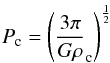 (1)where G is the gravitational constant and ρc the critical density.
Since a rotational period of 3.90 h is the critical rotational period, we can derive a lower limit to the density. The result based on our sample suggests a lower limit to the density of 0.71 g cm-3. Davidsson (1999, 2001) pointed out that the critical period in Eq. (1) is not a reliable estimate for true bodies and derived alternative expressions to Eq. (1). Using Davidsson’s expression for a low tensile strength of 0.01 MPa and a radius of 100 km, we obtain a lower limit to the density of 0.70 g cm-3.
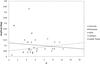 |
Fig. 3 Amplitude versus H for all objects presented in this work. Different symbols correspond to different object classifications. Thick line is a linear fit of all our sample of data. Dash line is a linear fit to all our sample of data except Varuna, Haumea and 2003 VS2 which exhibit a peak-to-peak amplitude >0.20 mag. |
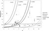 |
Fig. 4 Density versus H for all objects presented in this work. Different symbols correspond to different object classification. Dotted line is a linear fit. See text for definitions of the meaning of remaning. |
Another interesting subject is the plot of the amplitude of the variability as a function of the H parameter for each object presented in Fig. 3. One can immediately see the group of centaurs at large Hs and their amplitudes are apparently systematically above those from the regular TNOs (provided that the two very high amplitude TNOs are not taken into account). The centaur population lacks extremely low amplitude objects. In Fig. 3, two linear fits are shown: the thick line is a fit based on all our data. The dashed line is a linear fit to our data except for the objects with a peak to peak amplitude >0.20 mag (Varuna, Haumea and 2003 VS2). This fit clearly shows the trend of higher amplitude toward larger H objects.
Since a TNO is a triaxial ellipsoid with axes (a > b > c), one can determine that the lightcurve amplitude Δm varies according to the observational or viewing angle ξ (e.g., Binzel et al. 1989)  (2)The maximum of Eq. (2), corresponding to an observational angle of ξ = 90° (equatorial view), is obtained for a lightcurve amplitude:
  (3)Since we do not know the exact spin axis orientation of each object, or the observational angle, with Eq. (3) we can only compute a lower limit to a/b for each object. In other words, only a lower limit to the object elongation can be derived from the lightcurve amplitude. A lower limit to the density using the rotational period and the lower limit on the elongation of a body can be obtained by making use of the work of Chandrasekhar (1987) for fluid bodies. His work provides regions in the density and rotation rate space where different Jacobi shapes of varying elongations are allowed. It also shows that an ellipsoidal object with a/b > 2.31 is unstable. In Table 2, we present lower limits to the density of the bodies in this work based on the assumptions of hydrostatic equilibrium and that the variability is caused exclusively by shape effects. The validity of these assumptions are discussed below. Lower limits to the densities range from 0.22 g cm-3 for 2001 YH140 to 2.65 ± 0.43 g cm-3 for 2007 UL126. In other words, 2001 YH140 would have a Jacobi shape, if its density were at least 0.22 g cm-3. The average of the lower limits to the density of our sample is 0.90 g cm-3. But since we have a large enough sample, we can assume that the average viewing geometry of our bodies is 60°; thus we can derive not only lower limit to the a/b ratios, but almost true a/b ratios (in a statistically correct sense) by dividing them by sin(60°). In this way, the average density obtained from the increased elongations would be closer to the true mean density. The value we obtained in this case is 0.92 g cm-3. This value should be regarded as a very rough estimation because it is obvious that most of the lightcurves in this work are more significantly affected by albedo effects, than shape effects. A more adequate derivation of densities is presented in Duffard et al. (2009).
The density of an object depends on its internal composition. However, to explain the very low densities, ≲ 1 g cm-3, it is helpful to consider the concept of porosity. For example, Jewitt & Sheppard (2002), suggested that the low density of Varuna is due to porosity. Some objects have a higher density ≫ 1 g cm-3, which suggests that they are primarily composed of rock and ice. Objects of a high density and large diameter might have a core of rock and a mantle of ice. Lacerda et al. (2008) proposed that the high density of Haumea is consistent with this body being the core of a large differentiated body whose interior became exposed due to a large collision that completely eroded its mantle.
The density of all the objects as a function of the H parameter (a proxy for size) is shown in Fig. 4. A linear fit (Dotted line) shows almost no dependence on size. Based on a few TNOs whose Jacobi shape is very likely, Sheppard et al. (2008) suggested a relation between density and diameter: the largest objects (brightest) are denser than the smallest (faintest). The fit in Fig. 4 is not consistent with that idea, but one should keep in mind that most of the objects in our sample are probably MacLaurin spheroids, not Jacobi.
It is pertinent to assess whether the hydrostatic equilibrium assumption can be applicable to the objects in our sample. Tancredi & Favre (2008) addressed the issue of the minimum diameter needed for an object so that its mass can overcome the rigid body forces and thus adopt a hydrostatic equilibrium shape to become a dwarf planet, according to the 2006 IAU definition. As mentioned by Tancredi & Favre (2008), different criteria can be used. By integrating the hydrostatic differential equation with various assumptions one arrives at several expressions that relate the critical radius (R) for a self-gravitating body, the density (ρ), and the material strength (S). These equations can be collectively expressed  (4)where α can take several values according to the different criteria used (and ranges from α = 1 in the most simplistic case, to
  for a spherical body in more realistic cases). We note that a similar expression by Tancredi & Favre (2008) must contain a typo because the diameter in their equation should be radius.
One can express the size of a body using its albedo (p), absolute magnitude (Hv) and the magnitude of the Sun (Vsun). The diameter (D) is expressed in Russell (1916) as 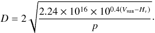 (5)Therefore, one can express the condition for hydrostatic equilibrium in terms of H, density, albedo and strength.
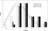 |
Fig. 5 Histograms of all our sample of data. We assume that all the lightcurves with amplitudes below an arbitrary limit are single peaked and those with amplitudes larger than this limit are double peaked. White data correspond to a limit of 0.10 mag, grey data correspond to a limit of 0.15 mag and black data correspond to a limit of 0.20 mag. Dash line is the Maxwellian fit to the distribution with 0.10 mag limit. Grey line is the Maxwellian fit to the distribution with 0.15 mag limit. Black line is the Maxwellian fit to the distribution with 0.20 mag limit. |
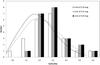 |
Fig. 6 Histograms of all TNOs presented in this work (our sample without the Centaurs). We assume that all the lightcurves with amplitudes below an arbitrary limit are single peaked and those with amplitude larger than this limit are double peaked. White data correspond to a limit of 0.10 mag, grey data correspond to a limit of 0.15 mag and black data correspond to a limit of 0.20 mag. Dashed line is the Maxwellian fit to the distribution with 0.10 mag limit. Grey line is the Maxwellian fit to the distribution with 0.15 mag limit. Black line is the Maxwellian fit to the distribution with 0.20 mag limit. Grey line falls on top of black line. |
In Fig. 4, we overplot the curves of density above which hydrostatic equilibrium is met, as a function of H. We considered three values of material strength: 0.01, 1, and 100 MPa. We chose two albedos values: 0.04 and 0.09. We note that Centaurs require a much lower material strength to be in hydrostatic equilibrium while TNOs may have more internal cohesion.
Finally, Figs. 5 and 6 are histograms of the rotation periods based on all our data and only the TNOs presented in this work, respectively. We assume that all the lightcurves with amplitudes below 0.15 mag are single peaked (which is almost equivalent to assuming that their rotational variation is caused mainly by albedo markings) and those with amplitudes larger than 0.15 mag are double peaked. In a first step, we used this arbitrary value which had already been used by several investigators. But, to determine if there is a more suitable value that marks the transition albedo-dominated lightcurves to shape-dominated lightcurves, we tested with limits of 0.10 mag from 0.20 mag.
In the case of asteroids, the distribution of rotation rates is Maxwellian (Binzel et al. 1989). A Maxwellian distribution has the form: ![Mathematical equation: \begin{equation} f(\Omega)=\sqrt{\frac{2}{\pi}}\frac{N\Omega^{2}}{\sigma^{3}}\exp\left[\frac{-\Omega^{2}}{2\sigma^{2}}\right] \end{equation}](/articles/aa/full_html/2010/14/aa12340-09/aa12340-09-eq112.png) (6)where Ω is the rotation rate (cycles/day) and N the total number of objects.
(6)where Ω is the rotation rate (cycles/day) and N the total number of objects.
A Maxwellian fit to the rotation rate distribution with the threshold of 0.1 mag gives values of 7.5 h (3.19 cycles/day) for the whole sample and 7.3 h (3.29 cycles/day) for the TNOs alone. A Maxwellian fit to the rotation rate distribution with the threshold of 0.15 mag infers values of 7.3 h (3.27 cycles/day) for the whole sample, 8.1 h (2.98 cycles/day) for the TNOs alone. A Maxwellian fit to the rotation rate distribution with the threshold of 0.20 mag gives values of 8 h (3 cycles/day) for the whole sample and 8.1 h (2.98 cycles/day) for the TNOs alone. With only 6 periods of Centaurs, we can’t give a satisfactory study. For these objects, we find a mean rotational value of 7.3 h. The confidence level of the chi-square test is higher for the threshold of 0.10 mag for the whole sample than for the TNOs alone.
None of the three different fits was significantly better than the others in terms of residuals because our sample of only 29 objects remains small for that purpose. Thus, we chose the intermediate 0.15 mag threshold as perhaps the most adequate one, based on our previous experience on asteroids and because a 0.15 mag variability is much easier to measure than 0.1 mag (and is therefore a good limit in terms of instrumental requirements). Fits to Maxwellian distributions of a larger sample are shown in Duffard et al. (2009), where the results of the present work and a compilation of the scientific literature are used.
If we do not fit any distribution but just consider the mean rotation periods of our objects, we obtain 7.5 h for the whole sample, 7.6 h for the TNOs alone, and 7.3 h for the Centaurs. These estimates may be more appropriate to compare with the average of 8.5 h quoted in Sheppard et al. (2008). Our values imply a more rapid rotation than previously derived.
6. Conclusions
We have presented a large sample of Kuiper belt Objects whose short-term variability has been studied in detail to increase the number of objects studied so far and try to avoid observational biases. Amplitudes and rotation periods have been derived for all of them with different degrees of reliability, but we have compiled an ensemble of all of them to study the whole population. We present therefore a homogeneous data set from which some conclusions can be drawn. We found that the percentage of low amplitude rotators is higher than previously thought and that in our sample the rotation rates appear to be slightly higher (faster objects) than previously suggested.
A simple idea investigated in detail in Duffard et al. (2009) to explain the large abundance of small amplitude objects might be that hydrostatic equilibrium is applicable to the overwhelming majority of the bodies and that the usual KBO shapes are MacLaurin spheroids which therefore do not cause any shape induced variations (and whose variability is caused by albedo variegations exclusively). We estimate that 0.1 mag seems to be a good measure of the typical variability caused by albedo features.
The plots of both amplitude versus size and rotation rate versus size seem to be compatible with the typical collisional evolution scenario in which larger objects have been only slightly affected by collisions, whereas the small fragments are highly collisionally evolved bodies with usually more rapid spins of larger amplitudes.
Based on the assumption of hydrostatic equilibrium, one can derive densities for all the bodies and we found a possible trend of higher densities toward higher sizes, which is a physically plausible scenario. There appears to be a spin barrier that allows us to obtain a density limit that is also compatible with the average density derived based on hydrostatic equilibrium assumptions. Nevertheless, a more appropriate derivation of mean densities is presented in Duffard et al. (2009).
Online material
Dates, geometric and photometric data of the observations.
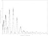 |
Fig. A.1 Lomb periodogram of 2003 FY128. |
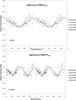 |
Fig. A.2 Rotational phase curve for 2003 FY128 obtained by using a spin period of 8.54 h (upper plot) and a spin period of 17.08 h (lower plot). The dash line is a Fourier Series fit of the photometric data. Different symbols correspond to different dates. |
 |
Fig. A.3 Rotational phase curves for 2003 MW12 obtained by using different spin periods; 5.9 h (upper plot) and 7.87 h (lower plot). In both case, we present a single peak lightcurve. The dash lines are a Fourier Series fits of the photometric data. Different symbols correspond to different dates. |
 |
Fig. A.4 Lomb periodogram of 2003 MW12. |
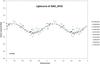 |
Fig. A.5 Rotational phase curve for 2003 OP32 obtained by using a spin period of 4.05 h. The dash line is a Fourier Series fit of the photometric data. Different symbols correspond to different dates. |
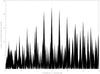 |
Fig. A.6 Lomb periodogram of 2003 OP32. |
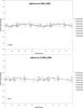 |
Fig. A.7 Rotational phase curves for 2004 SB60 obtained by using different spin periods: 6.09 h (upper plot) and 8.1 h (lower plot). In both cases, we present a single peak lightcurve. The dash lines are a Fourier Series fits of the photometric data. Different symbols correspond to different dates. |
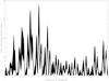 |
Fig. A.8 Lomb periodogram of 2004 SB60. |
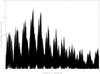 |
Fig. A.9 Lomb periodogram of 2005 CB79. |
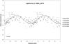 |
Fig. A.10 Rotational phase curve for 2005 CB79 obtained by using a spin period of 6.76 h. The dash line is a Fourier Series fit of the photometric data. Different symbols correspond to different dates. |
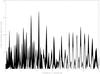 |
Fig. A.11 Lomb periodogram of 2005 RN43. |
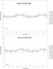 |
Fig. A.12 Rotational phase curves for 2005 RN43 obtained by using different spin periods: 5.62 h (upper plot) and 7.32 h (lower plot). In both case, we present a single peak lightcurve. The dash lines are a Fourier Series fits of the photometric data. Different symbols correspond to different dates. |
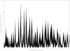 |
Fig. A.13 Lomb periodogram of 2005 RR43. |
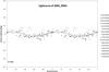 |
Fig. A.14 Rotational phase curve for 2005 RR43 obtained by using a spin period of 7.87 h. The dash line is a Fourier Series fit of the photometric data. Different symbols correspond to different dates. |
 |
Fig. A.15 Lomb periodogram of Quaoar. |
 |
Fig. A.16 Rotational phase curve for Quaoar obtained by using a spin period of 8.84 h for the single peak lightcurve (upper plot) and a spin period of 17.68 h (lower plot) for the double lightcurve. The dash lines are a Fourier Series fit of the photometric data. Different symbols correspond to different dates. |
 |
Fig. A.17 Lomb periodogram of Varuna. |
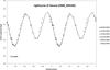 |
Fig. A.18 Rotational phase curve for Varuna obtained by using a spin period of 6.3418 h. The dash line is a Fourier Series fit of the photometric data. Different symbols correspond to different dates. |
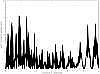 |
Fig. A.19 Lomb periodogram of 2002 AW197. |
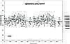 |
Fig. A.20 Rotational phase curve for 2002 AW197 obtained by using a spin period of 8.78 h. The dash line is a Fourier Series fit of the photometric data. Different symbols correspond to different dates. |
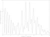 |
Fig. A.21 Lomb periodogram of 2002 TX300. |
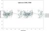 |
Fig. A.22 Rotational phase curve for 2002 TX300 obtained by using a spin period of 8.16 h. The dash line is a Fourier Series fit of the photometric data. Different symbols correspond to different dates. |
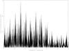 |
Fig. A.23 Lomb periodogram of Makemake. |
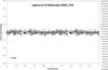 |
Fig. A.24 Rotational phase curve for Makemake obtained by using a spin period of 7.65 h. The thick line is a Fourier Series fit of the photometric data. Different symbols correspond to different dates. |
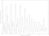 |
Fig. A.25 Lomb periodogram of 2001 YH140. |
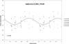 |
Fig. A.26 Rotational phase curve for 2001 YH140 obtained by using a spin period of 13.2 h. The dash line is a Fourier Series fit of the photometric data. Different symbols correspond to different dates. |
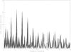 |
Fig. A.27 Lomb periodogram of Orcus. |
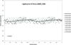 |
Fig. A.28 Rotational phase curve for Orcus obtained by using a spin period of 10.47 h. The dash line is a Fourier Series fit of the photometric data. Different symbols correspond to different dates. |
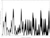 |
Fig. A.29 Lomb periodogram of 2002 VE95. |
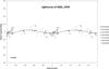 |
Fig. A.30 Rotational phase curve for 2002 VE95 obtained by using a spin period of 9.97 h. The dash line is a Fourier Series fit of the photometric data. Different symbols correspond to different dates. |
 |
Fig. A.31 Lomb periodogram of 2003 AZ84. |
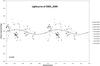 |
Fig. A.32 Rotational phase curve for 2003 AZ84 obtained by using a spin period of 6.79 h. The dash line is a Fourier Series fit of the photometric data. Different symbols correspond to different dates. |
 |
Fig. A.33 Lomb periodogram of 2003 VS2. |
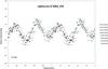 |
Fig. A.34 Rotational phase curve for 2003 VS2 obtained by using a spin period of 7.42 h. The dash line is a Fourier Series fit of the photometric data. Different symbols correspond to different dates. |
 |
Fig. A.35 Lomb periodogram of 2004 UX10. |
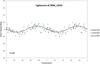 |
Fig. A.36 Rotational phase curve for 2004 UX10 obtained by using a spin period of 5.68 h. The dash line is a Fourier Series fit of the photometric data. Different symbols correspond to different dates. |
 |
Fig. A.37 Lomb periodogram of Haumea. |
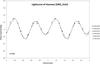 |
Fig. A.38 Rotational phase curve for Haumea obtained by using a spin period of 3.92 h. The dash line is a Fourier Series fit of the photometric data. Different symbols correspond to different dates. |
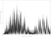 |
Fig. A.39 Lomb periodogram of 2005 RM43. |
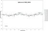 |
Fig. A.40 Rotational phase curve for 2005 RM43 obtained by using a spin period of 6.71 h. The dash line is a Fourier Series fit of the photometric data. Different symbols correspond to different dates. |
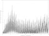 |
Fig. A.41 Lomb periodogram of Typhon. |
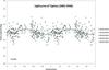 |
Fig. A.42 Rotational phase curve for Typhon obtained by using a spin period of 9.67 h. The dash line is a Fourier Series fit of the photometric data. Different symbols correspond to different dates. |
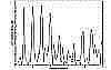 |
Fig. A.43 Lomb periodogram of 1996 TL66. |
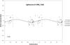 |
Fig. A.44 Rotational phase curve for 1996 TL66 obtained by using a spin period of 12 h. The dash line is a Fourier Series fit of the photometric data. Different symbols correspond to different dates. |
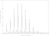 |
Fig. A.45 Lomb periodogram of Okyrhoe. |
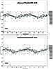 |
Fig. A.46 Rotational phase curves for Okyrhoe obtained by using different spin periods: 4.86 h (upper plot) and 6.08 h (lower plot). In both cases, we present a single peak lightcurve . The dash lines are a Fourier Series fits of the photometric data. Different symbols correspond to different dates. |
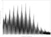 |
Fig. A.47 Lomb periodogram of 2005 UJ438. |
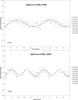 |
Fig. A.48 Rotational phase curve for 2005 UJ438 obtained by using a spin period of 4.16 h for the single peak lightcurve (upper plot) and a spin period of 8.32 h for the double peak lightcurve (lower plot). The dash line is a Fourier Series fit of the photometric data. Different symbols correspond to different dates. |
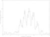 |
Fig. A.49 Lomb periodogram of 2007 UL126 (or 2002 KY14). |
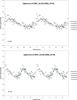 |
Fig. A.50 Rotational phase curves for 2007 UL126 (2002 KY14) obtained by using different spin periods: 3.56 h for the single peak lightcurve and 7.12 h for the double peak lightcurve. The dash lines are a Fourier Series fits of the photometric data. Different symbols correspond to different dates. |
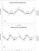 |
Fig. A.51 Rotational phase curves for 2007 UL126 (2002 KY14) obtained by using different spin periods: 4.2 h for a single peak lightcurve and 8.4 h for the double peak lightcurve. The dash lines are a Fourier Series fits of the photometric data. Different symbols correspond to different dates. |
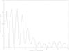 |
Fig. A.52 Lomb periodogram of Amycus. |
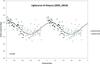 |
Fig. A.53 Rotational phase curve for Amycus obtained by using a spin period of 9.76 h. The dash line is a Fourier Series fit of the photometric data. Different symbols correspond to different dates. |
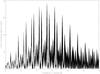 |
Fig. A.54 Lomb periodogram of 2003 CO1. |
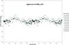 |
Fig. A.55 Rotational phase curve for 2003 CO1 obtained by using a spin period of 4.51 h. The dash line is a Fourier Series fit of the photometric data. Different symbols correspond to different dates. |
 |
Fig. A.56 Lomb periodogram of 2003 WL7. |
 |
Fig. A.57 Rotational phase curve for 2003 WL7 obtained by using a spin period of 8.24 h. The dash line is a Fourier Series fit of the photometric data. Different symbols correspond to different dates. |
 |
Fig. A.58 Lomb periodogram of 1999 TZ1. |
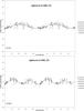 |
Fig. A.59 Rotational phase curve for 1999 TZ1 obtained by using a spin period of 5.211 h (upper plot) for the single peak lightcurve and 10.422 h (lower plot) for the double peak lightcurve. The dash line is a Fourier Series fit of the photometric data. Different symbols correspond to different dates. |
Acknowledgments
We are grateful to the Sierra Nevada Observatory, Calar Alto and INT staffs. This research was based on data obtained at the Observatorio de Sierra Nevada which is operated by the Instituto de Astrofísica de Andalucía, CSIC. This research is also based on observations collected at the Centro Astronómico Hispano Alemán (CAHA) at Calar Alto, operated jointly by the Max-Planck Institut für Astronomie and the Instituto de Astrofísica de Andalucía (CSIC). Other results were obtained at the Isaac Newton Telescope. The Isaac Newton Telescope is operated on the island of La Palma by the Isaac Newton Group in the Spanish Observatorio del Roque de Los Muchachos of the Instituto de Astrofísica de Canarias. This work was supported by contracts AYA2008-06202-C03-01 and AYA2005-07808-C03-01. R.D. acknowledges financial support from the MEC (contract Juan de la Cierva).
References
- Bauer, J. M., Meech, K. J., Fernández, Y. R., et al. 2003, Icarus, 166, 195 [NASA ADS] [CrossRef] [Google Scholar]
- Belskaya, I. N., Ortiz, J. L., Rousselot, P., et al. 2006, Icarus, 184, 277 [NASA ADS] [CrossRef] [Google Scholar]
- Benavidez, P. G., & CampoBagatin, A. 2009, Planet. Space Sci., 57, 201 [NASA ADS] [CrossRef] [Google Scholar]
- Binzel, R. P., Farinella, P., Zappala, V., & Cellino, A. 1989, in Asteroids II, ed. R. P. Binzel, T. Gehrels, & M. S. Matthews, 416 [Google Scholar]
- Brown, M. E., & Suer, T. 2007, IAU Circ., 8812, 1 [NASA ADS] [Google Scholar]
- Brown, M. E., Ragozzine, D., Stansberry, J., & Fraser, W. C. 2010, AJ, 139, 2700 [CrossRef] [Google Scholar]
- Chandrasekhar, S. 1987, Ellipsoidal figures of equilibrium (New York: Dover) [Google Scholar]
- Davidsson, B. J. R. 1999, Icarus, 142, 525 [NASA ADS] [CrossRef] [Google Scholar]
- Davidsson, B. J. R. 2001, Icarus, 149, 375 [NASA ADS] [CrossRef] [Google Scholar]
- Davis, D. R., & Farinella, P. 1997, Icarus, 125, 50 [NASA ADS] [CrossRef] [Google Scholar]
- Dotto, E., Perna, D., Barucci, M. A., et al. 2008, A&A, 490, 829 [NASA ADS] [CrossRef] [EDP Sciences] [Google Scholar]
- Duffard, R., Ortiz, J. L., Thirouin, A., Santos-Sanz, P., & Morales, N. 2009, A&A, 505, 1283 [NASA ADS] [CrossRef] [EDP Sciences] [Google Scholar]
- Farnham, T. L. 2001, IAU Circ., 7583, 4 [NASA ADS] [Google Scholar]
- Foster, G. 1995, AJ, 109, 1889 [NASA ADS] [CrossRef] [Google Scholar]
- Grundy, W. M., Noll, K. S., Virtanen, J., et al. 2008, Icarus, 197, 260 [NASA ADS] [CrossRef] [Google Scholar]
- Harris, A. W., Young, J. W., Bowell, E., et al. 1989, Icarus, 77, 171 [NASA ADS] [CrossRef] [Google Scholar]
- Holsapple, K. A. 2001, Icarus, 154, 432 [NASA ADS] [CrossRef] [Google Scholar]
- Holsapple, K. A. 2004, Icarus, 172, 272 [NASA ADS] [CrossRef] [Google Scholar]
- Jewitt, D. C., & Sheppard, S. S. 2002, AJ, 123, 2110 [NASA ADS] [CrossRef] [Google Scholar]
- Lacerda, P., & Luu, J. 2006, AJ, 131, 2314 [NASA ADS] [CrossRef] [Google Scholar]
- Lacerda, P., Jewitt, D., & Peixinho, N. 2008, AJ, 135, 1749 [NASA ADS] [CrossRef] [Google Scholar]
- Lagerkvist, C.-I., Harris, A. W., & Zappala, V. 1989, in Asteroids II, ed. R. P. Binzel, T. Gehrels, & M. S. Matthews, 1162 [Google Scholar]
- Lin, H.-W., Wu, Y.-L., & Ip, W.-H. 2007, Adv. Space Res., 40, 238 [NASA ADS] [CrossRef] [Google Scholar]
- Lomb, N. R. 1976, Ap&SS, 39, 447 [NASA ADS] [CrossRef] [Google Scholar]
- Luu, J. X., & Jewitt, D. C. 1998, ApJ, 494, L117 [NASA ADS] [CrossRef] [Google Scholar]
- Magnusson, P., & Lagerkvist, C.-I. 1991, A&AS, 87, 269 [NASA ADS] [Google Scholar]
- Morbidelli, A., Levison, H. F., Tsiganis, K., & Gomes, R. 2005, Nature, 435, 462 [NASA ADS] [CrossRef] [PubMed] [Google Scholar]
- Moullet, A., Lellouch, E., Doressoundiram, A., et al. 2008, A&A, 483, L17 [NASA ADS] [CrossRef] [EDP Sciences] [Google Scholar]
- Noll, K. S., Levison, H. F., Stephens, D. C., & Grundy, W. M. 2006, IAU Circ., 8751, 1 [NASA ADS] [Google Scholar]
- Ortiz, J. L., Gutiérrez, P. J., Casanova, V., & Sota, A. 2003a, A&A, 407, 1149 [NASA ADS] [CrossRef] [EDP Sciences] [Google Scholar]
- Ortiz, J. L., Gutiérrez, P. J., Sota, A., Casanova, V., & Teixeira, V. R. 2003b, A&A, 409, L13 [NASA ADS] [CrossRef] [EDP Sciences] [Google Scholar]
- Ortiz, J. L., Sota, A., Moreno, R., et al. 2004, A&A, 420, 383 [NASA ADS] [CrossRef] [EDP Sciences] [Google Scholar]
- Ortiz, J. L., Gutiérrez, P. J., Santos-Sanz, P., Casanova, V., & Sota, A. 2006, A&A, 447, 1131 [NASA ADS] [CrossRef] [EDP Sciences] [Google Scholar]
- Ortiz, J. L., Santos Sanz, P., Gutiérrez, P. J., Duffard, R., & Aceituno, F. J. 2007, A&A, 468, L13 [NASA ADS] [CrossRef] [EDP Sciences] [Google Scholar]
- Pravec, P., & Harris, A. W. 2000, Icarus, 148, 12 [NASA ADS] [CrossRef] [Google Scholar]
- Press, W. H., Teukolsky, S. A., Vetterling, W. T., & Flannery, B. P. 1992, Numerical recipes in FORTRAN, The art of scientific computing 2nd edition (Cambridge: University Press) [Google Scholar]
- Rabinowitz, D. L., Barkume, K., Brown, M. E., et al. 2006, ApJ, 639, 1238 [NASA ADS] [CrossRef] [Google Scholar]
- Rabinowitz, D. L., Schaefer, B. E., & Tourtellotte, S. W. 2007, AJ, 133, 26 [NASA ADS] [CrossRef] [Google Scholar]
- Rabinowitz, D. L., Schaefer, B. E., Schaefer, M., & Tourtellotte, S. W. 2008, AJ, 136, 1502 [NASA ADS] [CrossRef] [Google Scholar]
- Ragozzine, D., & Brown, M. E. 2007, AJ, 134, 2160 [NASA ADS] [CrossRef] [Google Scholar]
- Romanishin, W., & Tegler, S. C. 1999, Nature, 398, 129 [NASA ADS] [CrossRef] [Google Scholar]
- Russell, H. N. 1916, ApJ, 43, 173 [NASA ADS] [CrossRef] [Google Scholar]
- Sheppard, S. S. 2007, AJ, 134, 787 [NASA ADS] [CrossRef] [Google Scholar]
- Sheppard, S. S., & Jewitt, D. C. 2002, in Asteroids, Comets, and Meteors: ACM 2002, ed. B. Warmbein, ESA SP, 500, 21 [NASA ADS] [Google Scholar]
- Sheppard, S. S., & Jewitt, D. C. 2003, Earth Moon and Planets, 92, 207 [Google Scholar]
- Sheppard, S. S., Lacerda, P., & Ortiz, J. L. 2008, Photometric Lightcurves of Transneptunian Objects and Centaurs: Rotations, Shapes, and Densities, The Solar System Beyond Neptune, 129 [Google Scholar]
- Stetson, P. B. 1987, PASP, 99, 191 [NASA ADS] [CrossRef] [Google Scholar]
- Tancredi, G., & Favre, S. 2008, Icarus, 195, 851 [NASA ADS] [CrossRef] [Google Scholar]
- Tiscareno, M. S., & Malhotra, R. 2003, AJ, 126, 3122 [NASA ADS] [CrossRef] [Google Scholar]
- Trilling, D. E., & Bernstein, G. M. 2006, AJ, 131, 1149 [NASA ADS] [CrossRef] [Google Scholar]
All Tables
All Figures
|
Fig. 1 Rotational phase curve for 2003 FY128 obtained by using a spin period of 8.54 h (upper plot) and a spin period of 17.08 h (lower plot). The dash line is a Fourier series fit of the photometric data. Different symbols correspond to different dates. |
| In the text | |
|
Fig. 2 Rotational period versus H for all objects presented in this work. Different symbols correspond to different object classification. Dashed line defines a spin barrier. |
| In the text | |
|
Fig. 3 Amplitude versus H for all objects presented in this work. Different symbols correspond to different object classifications. Thick line is a linear fit of all our sample of data. Dash line is a linear fit to all our sample of data except Varuna, Haumea and 2003 VS2 which exhibit a peak-to-peak amplitude >0.20 mag. |
| In the text | |
|
Fig. 4 Density versus H for all objects presented in this work. Different symbols correspond to different object classification. Dotted line is a linear fit. See text for definitions of the meaning of remaning. |
| In the text | |
|
Fig. 5 Histograms of all our sample of data. We assume that all the lightcurves with amplitudes below an arbitrary limit are single peaked and those with amplitudes larger than this limit are double peaked. White data correspond to a limit of 0.10 mag, grey data correspond to a limit of 0.15 mag and black data correspond to a limit of 0.20 mag. Dash line is the Maxwellian fit to the distribution with 0.10 mag limit. Grey line is the Maxwellian fit to the distribution with 0.15 mag limit. Black line is the Maxwellian fit to the distribution with 0.20 mag limit. |
| In the text | |
|
Fig. 6 Histograms of all TNOs presented in this work (our sample without the Centaurs). We assume that all the lightcurves with amplitudes below an arbitrary limit are single peaked and those with amplitude larger than this limit are double peaked. White data correspond to a limit of 0.10 mag, grey data correspond to a limit of 0.15 mag and black data correspond to a limit of 0.20 mag. Dashed line is the Maxwellian fit to the distribution with 0.10 mag limit. Grey line is the Maxwellian fit to the distribution with 0.15 mag limit. Black line is the Maxwellian fit to the distribution with 0.20 mag limit. Grey line falls on top of black line. |
| In the text | |
|
Fig. A.1 Lomb periodogram of 2003 FY128. |
| In the text | |
|
Fig. A.2 Rotational phase curve for 2003 FY128 obtained by using a spin period of 8.54 h (upper plot) and a spin period of 17.08 h (lower plot). The dash line is a Fourier Series fit of the photometric data. Different symbols correspond to different dates. |
| In the text | |
|
Fig. A.3 Rotational phase curves for 2003 MW12 obtained by using different spin periods; 5.9 h (upper plot) and 7.87 h (lower plot). In both case, we present a single peak lightcurve. The dash lines are a Fourier Series fits of the photometric data. Different symbols correspond to different dates. |
| In the text | |
|
Fig. A.4 Lomb periodogram of 2003 MW12. |
| In the text | |
|
Fig. A.5 Rotational phase curve for 2003 OP32 obtained by using a spin period of 4.05 h. The dash line is a Fourier Series fit of the photometric data. Different symbols correspond to different dates. |
| In the text | |
|
Fig. A.6 Lomb periodogram of 2003 OP32. |
| In the text | |
|
Fig. A.7 Rotational phase curves for 2004 SB60 obtained by using different spin periods: 6.09 h (upper plot) and 8.1 h (lower plot). In both cases, we present a single peak lightcurve. The dash lines are a Fourier Series fits of the photometric data. Different symbols correspond to different dates. |
| In the text | |
|
Fig. A.8 Lomb periodogram of 2004 SB60. |
| In the text | |
|
Fig. A.9 Lomb periodogram of 2005 CB79. |
| In the text | |
|
Fig. A.10 Rotational phase curve for 2005 CB79 obtained by using a spin period of 6.76 h. The dash line is a Fourier Series fit of the photometric data. Different symbols correspond to different dates. |
| In the text | |
|
Fig. A.11 Lomb periodogram of 2005 RN43. |
| In the text | |
|
Fig. A.12 Rotational phase curves for 2005 RN43 obtained by using different spin periods: 5.62 h (upper plot) and 7.32 h (lower plot). In both case, we present a single peak lightcurve. The dash lines are a Fourier Series fits of the photometric data. Different symbols correspond to different dates. |
| In the text | |
|
Fig. A.13 Lomb periodogram of 2005 RR43. |
| In the text | |
|
Fig. A.14 Rotational phase curve for 2005 RR43 obtained by using a spin period of 7.87 h. The dash line is a Fourier Series fit of the photometric data. Different symbols correspond to different dates. |
| In the text | |
|
Fig. A.15 Lomb periodogram of Quaoar. |
| In the text | |
|
Fig. A.16 Rotational phase curve for Quaoar obtained by using a spin period of 8.84 h for the single peak lightcurve (upper plot) and a spin period of 17.68 h (lower plot) for the double lightcurve. The dash lines are a Fourier Series fit of the photometric data. Different symbols correspond to different dates. |
| In the text | |
|
Fig. A.17 Lomb periodogram of Varuna. |
| In the text | |
|
Fig. A.18 Rotational phase curve for Varuna obtained by using a spin period of 6.3418 h. The dash line is a Fourier Series fit of the photometric data. Different symbols correspond to different dates. |
| In the text | |
|
Fig. A.19 Lomb periodogram of 2002 AW197. |
| In the text | |
|
Fig. A.20 Rotational phase curve for 2002 AW197 obtained by using a spin period of 8.78 h. The dash line is a Fourier Series fit of the photometric data. Different symbols correspond to different dates. |
| In the text | |
|
Fig. A.21 Lomb periodogram of 2002 TX300. |
| In the text | |
|
Fig. A.22 Rotational phase curve for 2002 TX300 obtained by using a spin period of 8.16 h. The dash line is a Fourier Series fit of the photometric data. Different symbols correspond to different dates. |
| In the text | |
|
Fig. A.23 Lomb periodogram of Makemake. |
| In the text | |
|
Fig. A.24 Rotational phase curve for Makemake obtained by using a spin period of 7.65 h. The thick line is a Fourier Series fit of the photometric data. Different symbols correspond to different dates. |
| In the text | |
|
Fig. A.25 Lomb periodogram of 2001 YH140. |
| In the text | |
|
Fig. A.26 Rotational phase curve for 2001 YH140 obtained by using a spin period of 13.2 h. The dash line is a Fourier Series fit of the photometric data. Different symbols correspond to different dates. |
| In the text | |
|
Fig. A.27 Lomb periodogram of Orcus. |
| In the text | |
|
Fig. A.28 Rotational phase curve for Orcus obtained by using a spin period of 10.47 h. The dash line is a Fourier Series fit of the photometric data. Different symbols correspond to different dates. |
| In the text | |
|
Fig. A.29 Lomb periodogram of 2002 VE95. |
| In the text | |
|
Fig. A.30 Rotational phase curve for 2002 VE95 obtained by using a spin period of 9.97 h. The dash line is a Fourier Series fit of the photometric data. Different symbols correspond to different dates. |
| In the text | |
|
Fig. A.31 Lomb periodogram of 2003 AZ84. |
| In the text | |
|
Fig. A.32 Rotational phase curve for 2003 AZ84 obtained by using a spin period of 6.79 h. The dash line is a Fourier Series fit of the photometric data. Different symbols correspond to different dates. |
| In the text | |
|
Fig. A.33 Lomb periodogram of 2003 VS2. |
| In the text | |
|
Fig. A.34 Rotational phase curve for 2003 VS2 obtained by using a spin period of 7.42 h. The dash line is a Fourier Series fit of the photometric data. Different symbols correspond to different dates. |
| In the text | |
|
Fig. A.35 Lomb periodogram of 2004 UX10. |
| In the text | |
|
Fig. A.36 Rotational phase curve for 2004 UX10 obtained by using a spin period of 5.68 h. The dash line is a Fourier Series fit of the photometric data. Different symbols correspond to different dates. |
| In the text | |
|
Fig. A.37 Lomb periodogram of Haumea. |
| In the text | |
|
Fig. A.38 Rotational phase curve for Haumea obtained by using a spin period of 3.92 h. The dash line is a Fourier Series fit of the photometric data. Different symbols correspond to different dates. |
| In the text | |
|
Fig. A.39 Lomb periodogram of 2005 RM43. |
| In the text | |
|
Fig. A.40 Rotational phase curve for 2005 RM43 obtained by using a spin period of 6.71 h. The dash line is a Fourier Series fit of the photometric data. Different symbols correspond to different dates. |
| In the text | |
|
Fig. A.41 Lomb periodogram of Typhon. |
| In the text | |
|
Fig. A.42 Rotational phase curve for Typhon obtained by using a spin period of 9.67 h. The dash line is a Fourier Series fit of the photometric data. Different symbols correspond to different dates. |
| In the text | |
|
Fig. A.43 Lomb periodogram of 1996 TL66. |
| In the text | |
|
Fig. A.44 Rotational phase curve for 1996 TL66 obtained by using a spin period of 12 h. The dash line is a Fourier Series fit of the photometric data. Different symbols correspond to different dates. |
| In the text | |
|
Fig. A.45 Lomb periodogram of Okyrhoe. |
| In the text | |
|
Fig. A.46 Rotational phase curves for Okyrhoe obtained by using different spin periods: 4.86 h (upper plot) and 6.08 h (lower plot). In both cases, we present a single peak lightcurve . The dash lines are a Fourier Series fits of the photometric data. Different symbols correspond to different dates. |
| In the text | |
|
Fig. A.47 Lomb periodogram of 2005 UJ438. |
| In the text | |
|
Fig. A.48 Rotational phase curve for 2005 UJ438 obtained by using a spin period of 4.16 h for the single peak lightcurve (upper plot) and a spin period of 8.32 h for the double peak lightcurve (lower plot). The dash line is a Fourier Series fit of the photometric data. Different symbols correspond to different dates. |
| In the text | |
|
Fig. A.49 Lomb periodogram of 2007 UL126 (or 2002 KY14). |
| In the text | |
|
Fig. A.50 Rotational phase curves for 2007 UL126 (2002 KY14) obtained by using different spin periods: 3.56 h for the single peak lightcurve and 7.12 h for the double peak lightcurve. The dash lines are a Fourier Series fits of the photometric data. Different symbols correspond to different dates. |
| In the text | |
|
Fig. A.51 Rotational phase curves for 2007 UL126 (2002 KY14) obtained by using different spin periods: 4.2 h for a single peak lightcurve and 8.4 h for the double peak lightcurve. The dash lines are a Fourier Series fits of the photometric data. Different symbols correspond to different dates. |
| In the text | |
|
Fig. A.52 Lomb periodogram of Amycus. |
| In the text | |
|
Fig. A.53 Rotational phase curve for Amycus obtained by using a spin period of 9.76 h. The dash line is a Fourier Series fit of the photometric data. Different symbols correspond to different dates. |
| In the text | |
|
Fig. A.54 Lomb periodogram of 2003 CO1. |
| In the text | |
|
Fig. A.55 Rotational phase curve for 2003 CO1 obtained by using a spin period of 4.51 h. The dash line is a Fourier Series fit of the photometric data. Different symbols correspond to different dates. |
| In the text | |
|
Fig. A.56 Lomb periodogram of 2003 WL7. |
| In the text | |
|
Fig. A.57 Rotational phase curve for 2003 WL7 obtained by using a spin period of 8.24 h. The dash line is a Fourier Series fit of the photometric data. Different symbols correspond to different dates. |
| In the text | |
|
Fig. A.58 Lomb periodogram of 1999 TZ1. |
| In the text | |
|
Fig. A.59 Rotational phase curve for 1999 TZ1 obtained by using a spin period of 5.211 h (upper plot) for the single peak lightcurve and 10.422 h (lower plot) for the double peak lightcurve. The dash line is a Fourier Series fit of the photometric data. Different symbols correspond to different dates. |
| In the text | |
Current usage metrics show cumulative count of Article Views (full-text article views including HTML views, PDF and ePub downloads, according to the available data) and Abstracts Views on Vision4Press platform.
Data correspond to usage on the plateform after 2015. The current usage metrics is available 48-96 hours after online publication and is updated daily on week days.
Initial download of the metrics may take a while.