Detectability of extrasolar moons as gravitational microlenses

C. Liebig; J. Wambsganss

doi:10.1051/0004-6361/200913844

Home

All issues

Volume 520 (September-October 2010)

A&A, 520 (2010) A68

Full HTML

Free Access

Issue		A&A Volume 520, September-October 2010


Article Number		A68
Number of page(s)		13
Section		Planets and planetary systems
DOI		https://doi.org/10.1051/0004-6361/200913844
Published online		05 October 2010

A&A 520, A68 (2010)

Detectability of extrasolar moons as gravitational microlenses

C. Liebig - J. Wambsganss

Astronomisches Rechen-Institut, Zentrum für Astronomie der Universität Heidelberg, Mönchhofstraße 12-14, 69120 Heidelberg, Germany

Received 10 December 2009 / Accepted 25 April 2010

Abstract
We evaluate gravitational lensing as a technique for the detection of extrasolar moons. Since 2004 gravitational microlensing has been successfully applied as a detection method for extrasolar planets. In principle, the method is sensitive to masses as low as an Earth mass or even a fraction of it. Hence it seems natural to investigate the microlensing effects of moons around extrasolar planets. We explore the simplest conceivable triple lens system, containing one star, one planet and one moon. From a microlensing point of view, this system can be modelled as a particular triple with hierarchical mass ratios very different from unity. Since the moon orbits the planet, the planet-moon separation will be small compared to the distance between planet and star. Such a configuration can lead to a complex interference of caustics. We present detectability and detection limits by comparing triple-lens light curves to best-fit binary light curves as caused by a double-lens system consisting of host star and planet - without moon. We simulate magnification patterns covering a range of mass and separation values using the inverse ray shooting technique. These patterns are processed by analysing a large number of light curves and fitting a binary case to each of them. A chi-squared criterion is used to quantify the detectability of the moon in a number of selected triple-lens scenarios. The results of our simulations indicate that it is feasible to discover extrasolar moons via gravitational microlensing through frequent and highly precise monitoring of anomalous Galactic microlensing events with dwarf source stars.

Key words: gravitational lensing: micro - planets and satellites: general - methods: numerical - methods: statistical

1 Introduction

By now hundreds of extrasolar planets have been detected. For all we know, none of the newly discovered extrasolar planets offers physical conditions permitting any form of life. But the search for planets potentially harbouring life and the search for indicators of habitability is ongoing. One of these indicators might be the presence of a large natural satellite - a moon - which stabilises the rotation axis of the planet and thereby the surface climate (Benn 2001). It has also been suggested that a large moon itself might be a good candidate for offering habitable conditions (Scharf 2006). In the solar system, most planets harbour moons. In fact, the moons in the solar system outnumber the planets by more than an order of magnitude. No moon has yet been detected around an extrasolar planet.

The majority of known exoplanets has been discovered through radial velocity measurements, with the first successful finding reported by Mayor & Queloz (1995). This method is not sensitive to satellites of those planets, because the stellar ``Doppler wobble'' is only affected by the orbital movement of the barycentre of a planet and its satellites, though higher-order effects could play a role eventually. Here we consider Galactic microlensing, which has led to the discovery of several relatively low-mass exoplanets since the first report of a successful detection by Bond et al. (2004), as a promising technique for the search for exomoons.

As early as 1999, it has been suggested that extrasolar moons might be detectable through transit observations (Sartoretti & Schneider 1999), either through direct observation of lunar occultation or through transit timing variations, as the moon and planet rotate around their common barycentre, causing time shifts of the transit ingress and egress (cf. also Holman & Murray 2005). In their simulations of space-based gravitational microlensing Bennett & Rhie (2002) mention the possibility of discovering extrasolar moons similar to our own Moon. Later that year, Han & Han (2002) performed a detailed feasibility study whether microlensing offers the potential to discover an Earth-Moon analogue, but concluded that finite source effects would probably be too severe to allow detections. Williams & Knacke (2004) published the quite original suggestion to look for spectral signatures of Earth-sized moons in the absorption spectra of Jupiter-sized planets. Cabrera & Schneider (2007) proposed a sophisticated transit approach using ``mutual event phenomena'', i.e. photometric variation patterns due to different phases of occultation and light reflection of planet and satellite. Han (2008) undertook a new qualitative study of a number of triple-lens microlensing constellations finding ``non-negligible'' light curve signals to occur in the case of an Earth-mass moon orbiting a 10 Earth-mass planet, ``when the planet-moon separation is similar to or greater than the Einstein radius of the planet''. Lewis et al. (2008) analysed pulsar time-of-arrival signals for lunar signatures. Kipping (2009a,b) refined and extended the transit timing models of exomoons to include transit duration variations, and Kipping et al. (2009) examined transit detectability of exomoons with Kepler-class photometry and concluded that in optimal cases moon detections down to $0.2~M_{\rm Earth}$ should be possible.

We cover here several new aspects concerning the microlensing search for exomoons, extending the work of Han (2008). First, the detectability of lunar light curve perturbations is determined with a statistical significance test that does not need to rely on human judgement. Second, all parameters of the two-dimensional three-body geometry, including the position angle of the moon with respect to the planet-star axis, are varied. Third, an unbiased extraction of light curves from the selected scenarios enables a tentative prediction of the occurrence rate of detectable lunar light curve signals. A more detailed account of this study is available as Liebig (2009).

The paper is structured as follows: in Sect. 2, we recall the fundamental equations of gravitational microlensing relevant to our work. Our method for quantifying the detection rates for extrasolar moons in selected lensing scenarios is presented in Sect. 3. In Sect. 4, we discuss the astrophysical implications of the input parameters of the simulations. Our results are presented in Sect. 5, together with a first interpretation and a discussion of potential problems of our method.

2 Basics of gravitational microlensing

The deflection of light by massive bodies is a consequence of the theory of general relativity (Einstein 1916) and has been experimentally verified since 1919 (Dyson et al. 1920), see Paczynski (1996) for an introduction to the field or Schneider et al. (2006) for a comprehensive review.

The typical scale of angular separations in gravitational lensing is the Einstein radius $\theta _E$ , the angular radius of the ring of formally infinite image magnification that appears when a source at a distance $D_{\rm S}$ , a lens of mass Mat a distance $D_{\rm L}$ , and the observer are perfectly aligned:

$\displaystyle \theta_{E}= \sqrt{\frac{4GM}{c^2}\frac{D_{\rm LS}}{D_{\rm L} D_{\rm S}}},$

(1)

where G denotes the gravitational constant, c the speed of light. $D_{\rm LS}$ is the distance between lens plane and source plane; in the non-cosmological distance scale of our galaxy $D_{\rm LS} = D_{\rm S} - D_{\rm L }$ holds true. With the Einstein radius also comes the characteristic time scale of transient gravitational lensing events, the Einstein time $t_{\rm E} = D_{\rm L} \theta_{\rm E}/v_\perp$ with the transverse velocity $v_\perp$ of the lens relative to the source.

Here we focus on the triple lens case with host star (S), planet (P) and moon (M), see Fig. 1 for illustration. The lens equation can be expressed using complex coordinates, where $\eta$ shall denote the angular source position and $\xi$ the image positions, cf. choice of notation in Witt (1990) and Gaudi et al. (1998). $\xi_i$ stands for the angular position of the lensing body i. q_ij is the mass ratio between lenses i and j ( $q_{ij} = \frac{M_i}{M_{j}}$ ). The lens equation gets the following form, if the primary lens, the host star S, has unit mass and is placed in the origin of the lens plane,

$\displaystyle \eta = \xi - \frac{1}{\overline{\xi}} - \frac{q_{{\rm PS}}}{\over... ...\rm P}}}} - \frac{q_{{\rm MS}}}{\overline{\xi} - \overline{\xi_{{\rm M}}}}\cdot$

(2)

This is a mapping from the lens plane to the source plane, which maps the images of a source star to its actual position in the source plane. As pointed out in Rhie (1997), and explicitly calculated in Rhie (2002), the triple-lens equation is a tenth-order polynomial equation in $\xi$ .

In microlensing, the images cannot be resolved. Detectable is only the transient change in magnitude of the source star, when lens and source star are in relative motion to each other. The total magnification $\mu$ of the base flux is obtained as the inverse of the determinant of the Jacobian of the mapping Eq. (2),

$\displaystyle \mu = \frac{1}{\det J(\xi)} \textrm{, with } \det J(\xi)= 1-\frac... ...ial\eta}{\partial \bar{\xi}}\frac{\bar{\partial \eta}}{\partial \bar{\xi}}\cdot$

(3)

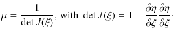
Gravitational lensing changes the apparent solid angle of a source, not the surface brightness. The magnification $\mu$ is the ratio of the total solid angle of the images and the apparent solid angle of the unlensed source.

For a status report of the past, present and prospective future of planet searching via Galactic microlensing the recent white papers of 2008/2009 are a good source of reference (Gaudi et al. 2009; Beaulieu et al. 2008; Dominik et al. 2008; Bennett et al. 2009).

3 Method

The simplest gravitational lens system incorporating an extrasolar moon is a triple-lens system consisting of the lensing star, a planet and a moon in orbit around that planet, as sketched in Fig. 1. Most likely, lunar effects will first show up as noticeable irregularities in light curves that have been initially observed and classified as light curves with planetary signatures. To measure the detectability of a given triple-lens system among binary lenses, we have to determine whether the provided triple-lens light curve differs statistically significantly from binary-lens light curves.

$\begin{figure} \par\includegraphics[width=8.8cm,clip]{13844fg01.eps} \end{figure}$

Figure 1:

Geometry of our triple-lens scenario, not to scale. Five parameters have to be fixed: the mass ratios $q_{\rm PS} = M_{\rm Planet}/M_{\rm Star}$ and $q_{\rm MP} = M_{\rm Moon}/M_{\rm Planet}$ , the angular separations in the lens plane $\theta _{\rm PS}$ and $\theta _{\rm MP}$ and the position angle of the moon $\phi$ . These parameters define uniquely the relative projected positions of the three bodies.

Open with DEXTER

To clarify the terminology: We investigate light curves that show a deviation from the single-lens case due to the presence of the planetary caustic, i.e. which would be modelled as a star-plus-planet system in a first approximation. We call lunar detectability the fraction of those light curves which display a significant deviation from a star-plus-planet lens model due to the presence of the moon. We measure the difference between a given triple-lens light curve (which is taken to be the ``true'' underlying light curve of the event) and its best-fit binary-lens counterpart. The best-fit binary-lens light curve is found by a least-square fit. We then employ $\chi ^2$ -statistics to see whether the triple-lens light curve could be explained as a normal fluctuation within the error boundaries of the binary-lens light curve. If this is not the case, the moon is considered detectable.

Detection and characterisation are two separate problems in the search for extrasolar planets or moons, though, and we do not make statements about the latter. When characterising an observed light curve with clear deviations from the binary model, it is still possible that ambiguous solutions - lunar and non-lunar - arise. This does not reflect on our results. We simply give the fraction of triple-lens light curves significantly deviating from binary-lens light curves, without exploring whether they can be uniquely characterised.

A qualitative impression of the lunar influence on the caustic structure can be gained from the magnification patterns in Fig. 2. Extracted example light curves are presented in Fig. 3. Going beyond the qualitative picture, in this paper we quantify the detectability of an extrasolar moon in gravitational microlensing light curves in selected scenarios.

$\begin{figure} \par\includegraphics[height=22cm,width=16.5cm,clip]{13844fg02.eps} \end{figure}$

Figure 2:

Details of the analysed triple-lens magnification maps for an example mass/separation scenario with $q_{\rm PS}= 10^{-3}$ , $q_{\rm MP}=10^{-2}$ , $\theta_{\rm PS}=1.3~\ensuremath{\theta_{E}}$ and $\theta_{\rm MP}=1.0~\ensuremath{\theta_{E}} ^P$ (the standard scenario as summarised in Table 1), showing the caustic configurations for twelve different lunar positions completing a full circular orbit in steps of 30 $\hbox {$^\circ $ }$ . The relative positions of star, planet and moon are sketched in the lower left of each panel (not to scale). The side lengths of the individual frames are $0.1~\ensuremath{\theta_{E}}$ . A darker shade of grey corresponds to a higher magnification. The straight black lines mark source trajectories, the resulting light curves are displayed in Fig. 3.

Open with DEXTER

$\begin{figure} \par\includegraphics[height=22cm,width=16.5cm,clip]{13844fg03.eps} \end{figure}$

Figure 3:

Sample of triple-lens light curves corresponding to the source trajectories depicted in Fig. 2. The solid light curves were extracted with an assumed solar source size, $R_{\rm Source} = R{_{\hbox {$\odot $ }}}$ ; the thin, dashed lines show the same light curves with $R_{\rm Source} = 3~R{_{\hbox{$\odot$ }}}$ . The magnification scale is given in negative magnitude difference ( $-\Delta$ mag), i.e. the unmagnified baseline flux of the source is 0. The time scale in units of the Einstein time t_E, assuming a uniform relative motion of source and lens.

Open with DEXTER

$\begin{figure} \par\includegraphics[width=8.5cm,clip]{13844fg04.eps} \end{figure}$

Figure 4:

Magnification pattern displaying the planetary caustic of a triple-lens system with mass ratios $q_{\rm PS}= 10^{-3}$ and $q_{\rm MP}=10^{-2}$ , corresponding, e.g., to an M-dwarf, a Saturn-mass planet and an Earth-mass satellite of that planet. Darker shades correspond to areas of higher magnification. The third body shows its influence as the small perturbation on the bottom cusp of the planetary caustic. The position angle of the moon is $\phi =90\hbox {$^\circ $ }$ , i.e. in the orientation of this map the moon is located above the planet. The complete set of parameters is given in Table 1. The side length of the pattern is $0.1~\theta_{E}$ in stellar Einstein radii. A source with radius $R_{\hbox {$\odot $ }}$ (2 $R_{\hbox {$\odot $ }}$ , 3 $R_{\hbox {$\odot $ }}$ , 5 $R_{\hbox {$\odot $ }}$ ) is indicated as a black disc (dashed circles) in the lower left. Taking the straight line that cuts the lunar perturbation of the caustic as the source trajectory of a solar sized source results in the light curve shown in Fig. 6 (solid line). Depending on the assumed source size, different light curves are obtained, see also Figs. 9a to c.

Open with DEXTER

3.1 Ray shooting

The triple-lens Eq. (2) is analytically solvable, but Han & Han (2002) pointed out that numerical noise in the polynomial coefficients caused by limited computer precision was too high ( $\sim10^{-15}$ ) when solving the polynomial numerically for the very small mass ratios of moon and star ( $\sim10^{-5}$ ). To avoid this, we employ the inverse ray-shooting technique, which has the further advantage of being able to account for finite source sizes and non-uniform source brightness profiles more easily. It also gives us the option of incorporating additional lenses (further planets or moons) without increasing the complexity of the calculations. This technique was developed by Schneider & Weiß (1986), Kayser et al. (1986) and Wambsganss (1990,1999) and already applied to planetary microlensing in Wambsganss (1997).

Inverse ray-shooting means that light rays are traced from the observer back to the source plane. This is equivalent to tracing rays from the background source star to the observer plane. The influence of all masses in the lens plane on the light path is calculated. In the thin lens approximation, the deflection angle is just the sum of the deflection angles of every single lens. After deflection, all light rays are collected in pixel bins of the source plane. Thus a magnification pattern is produced (e.g. Fig. 4). Lengths in this map can be translated to angular separations or, assuming a constant relative velocity between source and lens, to time intervals. The number of collected light rays per pixel is proportional to the magnification $\mu$ of a background source with pixel size at the respective position in the source plane. The resolution in magnification of these numerically produced patterns is finite and depends on the total number of rays shot.

3.2 Light curve simulation

We obtain simulated microlensing light curves with potential traces of a moon by producing magnification maps (Fig. 4) of triple-lens scenarios with mass ratios very different from unity. A light curve is then obtained as a one-dimensional cut through the magnification pattern, convolved with the luminosity profile of a star. Only a few more assumptions are necessary to simulate realistic, in principle observable, light curves: angular source size, relative motion of lens and source, and lens mass. As a first approximation to the surface brightness profiles of stars we use a profile with radius $R_{\rm Source}$ and constant surface brightness (ignoring limb-darkening effects). The light curve is sampled at equidistant intervals. In Sect. 4.7 we discuss physical implications of the sampling frequency. In order to be able to make robust statistical statements about the detectability of a moon in a chosen setting, i.e. a certain magnification pattern, we analyse a grid of source trajectories that delivers about two hundred light curves, see also Fig. 5. To have an unbiased sample, the grid is chosen independently of lunar caustic features, but all trajectories are required to show pronounced deviations from the single-lens light curve due to the planet.

$\begin{figure} \par\includegraphics[width=8.5cm,clip]{13844fg05.eps} \end{figure}$

Figure 5:

Illustration of how the magnification pattern of a given star-planet-moon configuration is evaluated. In order to have an unbiased statistical sample, the source trajectories are chosen independently of the lunar caustic features, though all light curves are required to pass through or close to the planetary caustic. This is realised through generating a grid of source trajectories that is only oriented at the planetary caustic. In the actual evaluation a 10 times denser grid than shown here was used. The magnification map has to be substantially larger than the caustic to ensure an adequate baseline for the light curve fitting. The side length of this pattern is $0.3~\theta_{E}$ , the position angle of the moon $\phi =90\hbox {$^\circ $ }$ , all other parameters are chosen as listed in Table 1. Source sizes of 1 $R_{\hbox {$\odot $ }}$ , 2 $R_{\hbox {$\odot $ }}$ , 3 $R_{\hbox {$\odot $ }}$ , and 5 $R_{\hbox {$\odot $ }}$ are indicated in the lower left.

Open with DEXTER

3.3 Fitting

For each triple-lens scenario, we produce an additional magnification pattern of a corresponding binary-lens system, where the mass of the moon is added to the planetary mass. As a first approximation, one can compare two light curves with identical source track parameters, see Fig. 6a. Numerically big differences can occur without a significant topological difference, because the additional third body not only introduces additional caustic features, it also slightly moves the location of the double-lens caustics.

$\begin{figure} \par\includegraphics[width=8.5cm,clip]{13844fg06.eps} \vspace*{-3mm} \end{figure}$

Figure 6:

Triple-lens light curve (solid line) extracted from the magnification pattern in Fig. 4, compared with a light curve extracted from the corresponding binary-lens magnification map (dashed line), with no third body and the planet mass increased by the previous moon mass. The difference of the two light curves is plotted as the dotted line. The central peak of the triple-lens light curve is caused by lunar caustic perturbations, that cannot easily be reproduced with a binary lens. In a), identical source trajectory parameters are used to extract the binary-lens light curve and large residuals remain that can be avoided with a different source trajectory. In b), the best-fit binary-lens light curve is shown (dashed) in comparison with the triple-lens light curve (solid). Here, the residuals can be attributed to the moon. If the deviation is significant, the moon is detectable in the triple-lens light curve. A source with solar radius at a distance of 8 kpc is assumed.

Open with DEXTER

Since the perturbation introduced by the moon is small, however, we have good starting conditions using the light curve from the binary magnification pattern that corresponds to the triple-lens magnification pattern. Keeping the planet-star separation fixed and changing the planetary mass to the sum of the masses of planet and moon, we are likely to be close to the global best-fit values. In our simplified approach, we only vary the source trajectory to search for the best-fitting binary-lens light curve, which already yields satisfactory results, as can be seen in Fig. 6b. For the fitting procedure we use the simple, straight-forward and robust least-square method.

3.4 Light curve comparison

We want to use the properties of the $\chi ^2$ -distribution for a test of significance of deviation between the two simulated light curves of the triple lens and the corresponding binary lens.

Most commonly, the $\chi ^2$ -distribution is used to test the goodness-of-fit of a model to experimental data. To compare two simulated curves instead, as in our case, one possible approach is to randomly generate artificial data around one of them and then consecutively fit the two theoretical curves to the artificial data with some free parameters. Two `` $\chi ^2$ -values'' Q²₁ and Q²₂will result. Their difference, $\Delta Q^2 = Q^2_1 - Q^2_2$ can then be calculated and a threshold value $\Delta Q^2_{\rm thresh}$ is chosen. The condition for reported detectability of the deviation is then $\Delta Q^2 > \Delta Q^2_{\rm thresh}$ . A detailed description of the algorithm and its application to microlensing was presented by Gaudi & Sackett (2000).

We decided to use a different approach here: In particular, we were led to consider other possible techniques by the wish to avoid ``feeding'' our knowledge of the data distribution to a random number generator in order to get an unbiased and random $\chi ^2$ -distributed sample of Q², when at the same time we have all the necessary information to calculate a much more representative $\chi ^2$ -value. We have developed a method to quantify significance of deviations between two theoretical functions that avoids the steps of data simulation and subsequent fitting.

Put simply, we calculate the mean $\langle Q^2\rangle$ of all `` $\chi ^2$ -values'' that would result, if data with a Gaussian scatter drawn from a triple-lens light curve is fitted with a binary light curve. If the triple-lens case and the best-fit binary-lens case are indistinguishable, then Q² will be $\chi ^2$ -distributed and $\langle Q^2\rangle$ will lie at or very close to $\langle \chi^2 \rangle = {\rm number~ of~ degrees~ of~ freedom}$ , the mean of the $\chi ^2$ probability density function. If the triple-lens light curve and the binary-lens light curve differ significantly, then Q² is not $\chi ^2$ -distributed and $\langle Q^2\rangle$ in particular will lie outside the expected range for $\chi ^2$ -distributed random variables. In the latter case, the moon is detectable. This approach is presented in mathematical detail in Appendix A.

4 Choice of scenarios

This section presents the assumptions that we use for our simulations. We discuss the astrophysical parameter space that is available for simulations of a microlensing system consisting of star, planet and moon. By choosing the most probable or most pragmatic value for each of the parameters, we create a standard scenario, summarised in Table 1 and visualised in Fig. 10, that all other parameters are compared against during the analysis.

The observational search for microlensing events caused by extrasolar planets is carried out towards the Galactic bulge, currently limited to the fields of the wide-field surveys OGLE (Udalski et al. 1992) and MOA (Muraki et al. 1999). This leads to some natural assumptions for the involved quantities. The source stars are typically close to the centre of the Galactic bulge at a distance of $D_{\rm S}=8$ kpc, where the surface density of stars is very high. For the distance to the lens plane we adopt a value of $D_{\rm L} = 6$ kpc. We assume our primary lens mass to be an M-dwarf star with a mass of $M_{\rm Star}=0.3~M_{\hbox{$\odot$ }}$ , because that is the most abundant type, cf. Fig. 5 of Dominik et al. (2008). Direct lens mass determination is only possible if additional observables, such as parallax, can be measured, cf. Gould (2009). We derive the corresponding Einstein radius of $\theta_{E}(D_{\rm S}, D_{\rm L}, M_{\rm Star}) = 0.32$ ms.

Five parameters describe our lens configuration, cf. Fig. 1: they are the mass ratios between planet and star $q_{\rm PS}$ and between moon and planet $q_{\rm MP}$ , the angular separations $\theta _{\rm PS}$ between planet and star and $\theta _{\rm MP}$ between moon and planet, and as the last parameter $\phi$ , the position angle of the moon with respect to the planet-star axis. These parameters are barely constrained by the physics of a three-body system, even if we do require mass ratios very different from unity and separations that allow for stable orbits.

The apparent source size $R_{\rm Source}$ and the sampling rate $f_{\rm sampled}$ affect the shape of the simulated light curves. We have to define an observational uncertainty $\sigma$ for the significance test in the final analysis of the light curves.

4.1 Mass ratio of planet and star q $_{\rm PS}$

We are interested in planets (and not binary stars). Accordingly, we want a small value for the mass ratio of planet and star $q_{\rm PS} = \frac{M_{\rm Planet}}{M_{\rm Star}}$ . Our standard value will be 10^-3 which is the mass ratio of Jupiter and Sun, or a Saturn-mass planet around an M-dwarf of $0.3~M\ensuremath{_{\hbox{$\odot$ }}}$ . At a given projected separation between star and planet, this mass ratio determines the size of the planetary caustic, with a larger $q_{\rm PS}$ leading to a larger caustic. $q_{\rm PS}$ is varied to also examine scenarios with mass ratios corresponding to a Jovian mass around an M-dwarf and to a Saturn mass around the Sun. Summarised: for the mass ratio between planet and star we use the three values $q_{\rm PS} = 3.3\times10^{-3}, 10^{-3}, 3\times10^{-4}$ .

4.2 Mass ratio of moon and planet q $_{\rm\sf MP}$

To be classified as a moon, the tertiary body must have a mass considerably smaller than the secondary. The standard case in our examination corresponds to the Moon/Earth mass ratio of $\frac{M_{\rm Moon}}{M_{\rm Earth}} = 10^{-2}$ . We are generous towards the higher mass end, and include a mass ratio of 10^-1 in our analysis, corresponding to the Charon/Pluto system. Both examples are singular in the solar system, but we argue that a more massive moon is more interesting, since it can effectively stabilise the obliquity of a planet, which is thought to be favouring the habitability of the planet (Benn 2001). At the low mass end of our analysis we examine $q_{\rm MP} = 10^{-3}$ . In Fig. 7, three different caustic interferences resulting from the three adopted mass ratios are shown. Summarised: For the mass ratio between moon and planet we use the three values $q_{\rm MP} = 10^{-3}, 10^{-2}, 10^{-1}$ .

4.3 Angular separation of planet and star $\theta _{\rm PS}$

The physical separation of a planet and its host star, i.e. the semi-major axis $a_{\rm PS}$ , is not directly measurable in gravitational lensing. Only the angular separation $\theta _{\rm PS}$ can directly be inferred from an observed light curve, where $0 \le \theta_{\rm PS}D_{\rm L} \le a_{\rm PS}$ is valid for a given physical separation $a_{\rm PS}$ at a lens distance $D_{\rm L}$ . The angular separation $\theta _{\rm PS}$ of a binary will evoke a certain topology of caustics, illustrated e.g. in Fig. 1 of Cassan (2008). They gradually evolve from the close separation case with two small triangular caustics on the far side of the star and a small central caustic at the star position, to a large central caustic for the intermediate case, when the planet is situated near the stellar Einstein ring, $\theta_{\rm PS}=1.0~\ensuremath{\theta_{E}}$ . This is also called the ``resonant lensing'' case, as described in Wambsganss (1997). If the planet is moved further out, one obtains a small central caustic and a larger isolated, roughly kite-shaped planetary caustic that is elongated towards the primary mass in the beginning, but becomes more and more symmetric and diamond-shaped if the planet is placed further outwards.

$\begin{figure} \par\mbox{\subfigure[$q_{\rm MP}=10^{-3}$ ]{\includegraphics[widt... ... ]{\includegraphics[width=3cm]{13844fg07c.eps} }}\vspace*{-3.5mm} \end{figure}$

Figure 7:

Caustic topology with different lunar mass ratios. From left to right, the lunar mass ratio increases from $q_{\rm MP} = 10^{-3}$ to 10^-1. The side length of the displayed patterns is $0.05~\ensuremath{\theta_{E}}$ . All other parameters as given in Table 1, in particular $q_{\rm PS}= 10^{-3}$ and $\theta_{\rm MP}=1.0~\ensuremath{\theta_{E}} ^P$ . Source sizes of $1~R{_{\hbox{$\odot$ }}}$ to $5~R\ensuremath{_{\hbox{$\odot$ }}}$ are indicated in the lower left.

Open with DEXTER

In analogy, a ``lunar resonant lensing zone'' can be defined, when measuring the angular separation of moon and planet in units of planetary Einstein radii $\ensuremath{\theta_{E}} ^P = \sqrt{q_{\rm PS}}~\ensuremath{\theta_{E}}$ . Viewing our solar system as a gravitational lens system at $D_{\rm L} = 6$ kpc and with $D_{\rm S}=8$ kpc, Jupiter's Einstein radius in physical lengths would be 0.11 AU in the lens plane, that is almost 10 times the semi-major axis of Callisto. However, the smaller moons of Jupiter cover the region out to 2 Jovian Einstein radii. If there is a moon at an angular separation of the planet of $0.6~\ensuremath{\theta_{E}} ^P\la \theta_{\rm MP} \la 3.0~\ensuremath{\theta_{E}} ^P$ , it will show its influence in any of the caustics topologies. But we focus our study on the wide-separation case for the following reasons: regarding the close-separation triangular caustics, we argue that the probability to cross one of them is vanishingly small and, furthermore, the magnification substantially decreases as they move outwards from the star. The intermediate or resonant caustic is well ``visible'' because it is always located close to the peak of the single-lens curve. But all massive bodies of a given planetary system affect the central caustic with minor or major perturbations and deformations (Gaudi et al. 1998). There is no reason to expect that extrasolar systems are generally less densely populated by planets or moons than the solar system. Since we are looking for very small deviations, identifying the signature of the moon among multiple features caused by low-mass planets and possibly more moons would be increasingly complex. The wide-separation case is most favourable, because the planetary caustic is typically caused by a single planet and interactions due to the close presence of other planets are highly unlikely (Bozza 2000,1999). Any observed interferences can therefore be attributed to satellites of the planet. Planets with only one dominant moon are at least common in the solar system (Saturn & Titan, Neptune & Triton, Earth & Moon). Such a system would be the most straightforward to detect in real data.

This makes a strong case for concentrating on the wide-separation planetary caustic. As the standard we choose a separation of $\theta_{\rm PS}=1.3~\ensuremath{\theta_{E}}$ and also test a scenario with $\theta_{\rm PS}=1.4~\ensuremath{\theta_{E}}$ . For comparison: the maximum projected separation of Jupiter at the chosen distances $D_{\rm S}$ and $D_{\rm L}$ corresponds to 1.5 solar Einstein radii. Summarised: for the angular separation between planet and star we use the two values $\theta_{\rm PS} = 1.3\theta_E, 1.4\theta_E$ .

4.4 Angular separation of moon and planet $\theta _{\rm MP}$

As the moon by definition orbits the planet, there is an upper limit to the semi-major axis of the moon $a_{\rm MP}$ . It must not exceed the distance between the planet and its inner Lagrange point. This distance is called Hill radius and is calculated as

$\begin{displaymath}r_{\rm Hill}= a_{\rm PS} \left(\frac{M_{\rm P}}{3M_{\rm S}}\right)^{\frac{1}{3}} \end{displaymath}$

for circular orbits, with the semi-major axis $a_{\rm PS}$ of the planetary orbit. This can be translated to ``lensing parameters'', but the equation changes into the inequality

$\displaystyle r_{\rm Hill} \ge \theta_{\rm PS} D_{\rm L} \left(\frac{1}{3} q_{\rm PS}\right)^{\frac{1}{3}},$

(4)

because for a physical distance $a_{\rm PS}$ , the apparent (i.e. projected) separation lies in the range $0 \le \theta_{\rm PS}D_{\rm L} \le a_{\rm PS}$ depending on the inclination towards the line of sight. Thus, the Hill radius constraint $a_{\rm MP} \le r_{\rm Hill}$ cannot be regarded as a strict limit. Though, turning this argument around, a minimum region of secured stability exists for given mass ratios and angular planet-star separation $\theta _{\rm PS}$ . Bodies in prograde motion with an orbit below $0.5~r_{\rm Hill}$ can have long term stability, for retrograde motion the limit is somewhat higher at $0.75~r_{\rm Hill}$ (see Domingos et al. 2006, and references therein, particularly; Hunter 1967). The region of secured stability for our standard scenario has a radius of

$\begin{displaymath}\theta_{\rm MP} \le 0.5\times \theta_{\rm PS}D_{\rm L} \left(... ...{\frac{1}{3}} = 0.045~ {\theta_{E}} = 1.53~ {\theta_{E}}^{P}, \end{displaymath}$

which leads to $a_{\rm MP} = 0.09$ AU in our setting. Our choice of $\theta _{\rm MP}$ is also motivated by a desire to have caustic interactions between lunar and planetary caustic, a resonance, because only under this condition the moon will give rise to light curve features that are distinctly different from those of a low-mass planet. If the moon is located at an angular separation from the planet of - depending on the position angle of the moon - roughly $0.6~\ensuremath{\theta_{E}} ^P\la \theta_{\rm MP} \la 3.0~\ensuremath{\theta_{E}} ^P$ , it will influence the planetary caustic. For angular separations larger than $3.0~\ensuremath{\theta_{E}} ^P$ , the lunar caustic barely influences the planetary caustic, and if it is detected, it will be detected as a distinct secondary caustic. Han (2008) already pointed out that the lunar signal does not vanish with an increased separation from the planet. But the lunar mass might be wrongly identified as a second, lower-mass planet rather than a satellite of the first planet. For comparison, the major moons of the solar system are all at considerably smaller angular separations than 1.0 $\ensuremath{\theta_{E}} ^P$ , if observed as a gravitational lens system from $D_{\rm L} = 6$ kpc with $D_{\rm S}=8$ kpc, with our Moon being most favourable at 0.4 of Earth's Einstein radii at maximum projected separation. But as we have learnt through the discovery of hundreds of exoplanets, we do not have to expect solar system properties to be mirrored in exoplanetary systems.

We focus on configurations with strong interferences of planetary and lunar caustic, what one might call the ``resonant case of lunar lensing'', examples of which are displayed in Fig. 8. Therefore, our standard case will have an angular separation of moon and planet of one planetary Einstein radius. In total, we evaluate four settings: $\theta_{\rm MP} = 0.8 \theta_{E}^P, 1.0 \theta_{E}^P, 1.2 \theta_{E}^P, 1.4 \theta_{E}^P$ , in the chosen setting (Table 1), this corresponds to physical projected separations from 0.5 to 0.8 AU.

$\begin{figure} \par\mbox{\subfigure[$\theta_{\rm MP}=0.8~\ensuremath{\theta_{E}}... ... ]{ \includegraphics[width=3cm]{13844fg08c.eps} } }\vspace*{-4mm} \end{figure}$

Figure 8:

Magnification patterns with side lengths of $0.05~\ensuremath{\theta_{E}}$ showing the lunar perturbation of the planetary caustic for increasing angular separations of moon and planet of $\theta_{\rm MP}= 0.8~\ensuremath{\theta_{E}} ^P, 1.0~\ensuremath{\theta_{E}} ^P, 1.2~\ensuremath{\theta_{E}} ^P$ , while all other parameters are as in Table 1. The topology of interaction varies with the angular separation. Source sizes of $1~R\ensuremath{_{\hbox{$\odot$ }}}$ to $5~R\ensuremath{_{\hbox{$\odot$ }}}$ are indicated in the lower left.

Open with DEXTER

4.5 Position angle of moon $\phi$

The fifth physical parameter for determining the magnification patterns is the position angle of the moon $\phi$ with respect to planet-star axis, as depicted in Fig. 1. It is the only parameter that is not fixed in our standard scenario. Instead, we evaluate this parameter in its entirety by varying it in steps of $30\hbox{$^\circ$ }$ to complete a full circular orbit of the moon around the planet. By doing this, we are aiming at getting complete coverage of a selected mass/separation scenario. Figure 2 visualises how the position of the moon affects the planetary caustic. It is not to be expected that we will ever have an exactly frontal view of a perfectly circular orbit, but it serves well as a first approximation. Summarised: we choose 12 equally spaced values for the position angle $\phi$ of the moon relative to the planet-star axis, and the results for the various parameter sets are averaged over these 12 geometries.

4.6 Source size R $_{\rm Source}$

The source size strongly influences the amplitudes of the light curve fluctuations and the ``time resolution''. Larger sources blur out finer caustic structures, compare Fig. 9. For our source star assumptions, we have to take into account not only stellar abundances, but also the luminosity of a given stellar type. Main sequence dwarfs are abundant in the Galactic bulge, but they are faint, with apparent magnitudes of $\sim$ 15 mag to 25 mag at $D_{\rm S}=8$ kpc. In the crowded microlensing fields, they are difficult to observe with satisfying photometry by ground-based telescopes, even if they are lensed and magnified. Giant stars, with apparent baseline magnitudes $\sim$ 13 mag to 17 mag, are more likely to allow precise photometric measurements from ground and, therefore, today's follow-up observations are biased towards these source stars.

The finite source size constitutes a serious limitation to the discovery of extrasolar moons. In fact, Han & Han (2002) stated that detecting satellite signals in the lensing light curves will be close to impossible, because the signals are smeared out by the severe finite-source effect. They tested various source sizes (and planet-moon separations) for an Earth-mass planet with a Moon-mass satellite. They find that even for a K0-type source star ( $R_{\rm Source} = 0.8~R_{\hbox{$\odot$ }}$ ) any light curve modifications caused by the moon are washed out. Han (2008) increased lens masses and by assuming a solar source size $R_{\rm Source} = R{_{\hbox {$\odot $ }}}$ , he finds that ``non-negligible satellite signals occur'' in the light curves of planets of 10 to 300 Earth masses, ``when the planet-moon separation is similar to or greater than the Einstein radius of the planet'' and the moon has the mass of Earth. We use a solar sized source as our standard case, and present results for four more source radii: $R_{{\rm Source}} = 1~R_{\hbox{$\odot$ }}, 2~R_{\hbox{$\odot$ }}, 3~R_{\hbox{$\odot$ }}, 5~R_{\hbox{$\odot$ }}, 10~R_{\hbox{$\odot$ }}$ . In terms of stellar Einstein radii this corresponds to five different source size settings from $1.8 \times 10^{-3}~\ensuremath{\theta_{{E}}}$ to $18 \times 10^{-3}~\ensuremath{\theta_{{E}}}$ .

The ability to monitor smaller sources - dwarfs, low-mass main sequence stars - with good photometric accuracy is one of the advantages of space-based observations. Hence a satellite mission is the ideal tool for this aspect of microlensing, routine detections of moons around planets can be expected with a space-based monitoring program on a dedicated satellite.

$\begin{figure} \par\includegraphics[width=8.5cm,clip]{13844fg9.eps} \vspace*{-2.5mm} \end{figure}$

Figure 9:

Illustration of the increasing source radius, compare Fig. 6b: a) $R_{\rm source} = 2_{\hbox {$\odot $ }}$ , b) $3~R_{\hbox{$\odot$ }}$ , and c) $5~R_{\hbox{$\odot$ }}$ , all other parameters as given in Table 1. The triple-lens light curve (solid) is obtained from the magnification pattern in Fig. 4, the best-fit binary-lens light curve (dashed) from the corresponding magnification pattern without a moon. The difference between the two curves is plotted as a dotted line.

Open with DEXTER

4.7 Sampling rate f $_{\rm sampled}$

Typical exposure times for the microlensing light curves are 10 to 300 s at a 1.5 m telescope. The frequency of observations of an individual interesting event varies between once per 2 h to once every few minutes, for a single observing site only limited by exposure time and read-out time of the instrument. One example of this is the peak coverage of MOA-2007-BLG-400, see Dong et al. (2009), where frames were taken every six minutes. Higher observing frequency equals better coverage of the resulting light curve. A normal microlensing event is seen as a transient brightening that can last for a few days to weeks or even months. A planet will alter the light curve from fraction of a day to about a week; the effect of a low-mass planet or a moon will only last for a few hours or shorter, see e.g. Beaulieu et al. (2006). This duration is inversely proportional to the transverse velocity $v_\perp$ with which the lens moves relative to the line of sight or the relative proper motion $\mu_\perp$ between the background source and the lensing system. We fix this at a typical $v_{\perp} = 200$ km s^-1 for $D_{\rm L} = 6$ kpc or $\mu_{\perp} = 7.0~{\rm mas/year}$ .

For the simulations, a realistic, non-continuous observing rate is mimicked by evaluating the simulated light curve at intervals that correspond to typical frequencies, but allowing for a constant sampling rate, which in practise is often prohibited by observing conditions. We sample the triple-lens light curve in equally sized steps. With the assumed constant relative velocity, this translates to equal spacing in time. Aiming for a rate of $f_{\rm sampled} \simeq \frac{1 {\rm frame}}{15~{\rm min}}$ , we choose a step size of $6 \times 10^{-4}~\ensuremath{\theta_{E}}$ . To see the effect of a decreased sampling rate, we have also examined the standard scenario (see Table 1) with sampling rates of factors of 1.5 and 2 longer. Summarised: we use three different sampling rates, $f_{\rm sampled} = 1/15$ min, 1/22 min, 1/30 min.

4.8 Assumed photometric uncertainty $\sf\sigma$

The standard error $\sigma$ of a data point in a microlensing light curve can vary significantly. Values between 5 and 100 mmag seem realistic, see, e.g., data plots in the recent event analyses of Gaudi et al. (2008) or Janczak et al. (2009). The photometric uncertainty directly enters the statistical evaluation of each light curve as described in Appendix A. We have drawn results for an (unrealistically) broad $\sigma$ -range from 0.5 mmag to 500 mmag. An error as small as $\sigma = 0.5$ mmag for a V=12.3star has recently been reached with high-precision photometry of an exoplanetary transit event at the Danish 1.54 m telescope at ESO La Silla (Southworth et al. 2009), which is one of the telescopes presently used for Galactic microlensing monitoring observations, but this low uncertainty cannot be transferred to standard microlensing observations, where crowded star fields make e.g. the use of defocussing techniques impossible. In our discussion, we regard only the more realistic range from $\sigma = 5$ to 100 mmag. We adopt an ideal scenario with a fixed $\sigma$ -value for all sampled points on the triple-lens light curve and set $\sigma = 20$ mmag to be our standard for the comparison of different mass and separation scenarios. Summarised: we explore 5 values as photometric uncertainty: $\sigma = 5$ , 10, 20, 50, 100 mmag.

Table 1: Parameter values of our standard scenario.

$\begin{figure} \par\includegraphics[width=16cm,clip]{13844fg10.eps}\vspace*{-2mm} \end{figure}$

Figure 10:

Visualisation of the approximate lunar resonance zone (dark-grey ring), where planetary and lunar caustic overlap and interact. Also depicted is the planet lensing zone (light grey), which is the area of planet positions for which the planetary caustic(s) lie within the stellar Einstein radius. Distances and caustic inset are to scale. The physical scale depends not only on the masses of the lensing bodies, but also on the distances to the lens system and the background star. In our adopted standard scenario, cf. Table 1, the Einstein radius $\theta _E$ corresponds to 1.9 AU in the lens plane. This places the planet at a projected orbit radius of 2.5 AU, whereas the moon's orbit has a radius of 0.06 AU (corresponding to one planetary Einstein radius). The lunar resonance zone covers lunar orbit radii from 0.04 AU to 0.18 AU.

Open with DEXTER

5 Results: detectability of extrasolar moons in microlensing light curves

The numerical results of our work are presented and a first interpretation is made. We start by considering the result for a single magnification pattern in Sect. 5.1. We then present results that cover specific physical triple-lens scenarios (Sect. 5.2). We also evaluate the parameter dependence of the detectability rate, by varying each parameter separately.

5.1 Evaluation of a single magnification pattern

As described in Sect. 3, all magnification maps are evaluated by taking a large sample of unbiased light curves and then determining the fraction of light curves with significant lunar signals. The results for a single magnification map (here the pattern from Fig. 5), are displayed in Table 2.

Table 2: Detectability of the third mass in the magnification pattern of Fig. 5, for different assumed photometric uncertainties.

The percentages can be interpreted as the ``detection probability'' of the moon in a random observed light curve displaying a signature of the planetary caustic - ignoring the possible complication to fully characterise the signal. In this map, the detectability of the moon is about one third, provided we have an observational uncertainty of $\sigma = 20$ mmag. Obviously, with a larger photometric error, one is less sensitive to small deviations caused by the moon.

5.2 Results for selected scenarios

In order to be able to make general statements about a given planetary/lunar system, we average the results for 12 magnification patterns representing a full lunar orbit with $\phi=0\hbox{$^\circ$ }, 30\hbox{$^\circ$ },\ldots, 330\hbox{$^\circ$ }$ .

5.2.1 Variation of the photometric uncertainty

The scenario described in Table 1 is evaluated for different photometric uncertainties by analysing the 12 magnification maps shown in Fig. 2. The results are displayed in Table 3.

Table 3: Detectability of the moon in our standard scenario as a function of assumed photometric uncertainty.

For an photometric uncertainty of $\sigma = 20$ mmag, the result is that about 30% of the light curves show significant deviations from a best-fit binary-lens light curve and display detectable signs of the moon. We recall again our requirements:

the host planet of the satellite has been detected;
a small source size, up to a few solar radii, is required;
the moon is massive compared to satellites in the solar system;
we have assumed light curves with a constant sampling rate of one frame every 15 min for about 50 to 70 h.

As would be expected, the detection rate increases with higher photometric sensitivity and decreases with a larger uncertainty. At a photometric error of 20 mmag or worse, the detection of a moon depends on whether the source trajectory passes through or close to the lunar caustic. The finite magnification resolution of the magnification patterns induces an uncertainty in the detectability results that increases with smaller $\sigma$ -values, but it is negligible for the examined range.

5.2.2 Changing the angular separation of planet and moon

Table 4 lines up the changing detectability for different values of the projected planet-moon separation $\theta _{\rm MP}$ , with all other parameters as in standard scenario (Table 1).

Table 4: Detectability of the moon as a function of the planet-moon separation for our standard scenario.

With the chosen range from $\theta_{\rm MP}=0.8~\ensuremath{\theta_{E}} ^P$ to $1.4~\ensuremath{\theta_{E}} ^P$ , we are within the regime of caustic interactions of planetary and lunar caustic. We find that the percentage of detectability is almost constant at a 30% level. Han (2008) defines regions of possible satellite detections as the region of angular moon-planet separations between the lower limit of one planetary Einstein radius and an upper limit at the projected Hill-radius average. From our results, we conclude that detections with $\theta_{\rm MP} < 1.0~\ensuremath{\theta_{E}} ^P$ are well possible. We have not fully probed the lower limit region, but for $\theta_{\rm MP} < 0.5~\ensuremath{\theta_{E}} ^P$ the size of the lunar caustic perturbation decreases substantially.

5.2.3 Variation of the moon mass

Table 5 shows the changing detectability for a varying mass ratio $q_{\rm MP}$ of lunar and planetary mass, with all other parameters as in our standard scenario (Table 1).

Table 5: Detectability of the moon depending on moon-planet mass ratio.

Over the range of the moon-planet mass ratio, $q_{\rm MP} = 10^{-3}$ , 10^-2, and 10^-1 the detection rate increases from 2.4% to 85.6%, compare also Fig. 7. Not surprisingly: the more massive the moon, the easier it is to detect.

5.2.4 Changing the planetary mass ratio

Table 6 lists the changing detectability for a varying mass ratio between planet and star $q_{\rm PS}$ .

Table 6: Dependence of lunar detectability as a function of the planet-star mass ratio, all other parameters as in our standard scenario.

We adjusted the parameters of the grid of source trajectories, so that the grid spacing scales with the total caustic size. For a decreasing mass of the planet, the apparent source size increases relative to the caustic size, so finer features will be blurred out more in the case of a smaller planet. Also the absolute change in magnification scales with the planetary mass. As expected, the detection efficiency is roughly proportional to the planetary caustic size.

5.2.5 Different sampling rates

Table 7 presents the changing lunar detectability for different sampling rates.

Table 7: Detectability of the moon depending on the sampling rate of the simulated light curves.

A lower sampling frequency lowers the detection probability, but the effect is less pronounced than expected. This means it may be favourable to monitor a larger number of planetary microlensing events with high sampling frequency, rather than a very small number of them with ultra-high sampling. Our assumed sampling rates can easily be met by follow-up observations, as they are presently performed for anomalous Galactic microlensing events.

5.2.6 Source size variations

We analysed simulated light curves of the standard scenario with five different source star radii. They cover the range between a star the size of our Sun and a small giant star with $R_{\rm Source} = 10~R_{\hbox{$\odot$ }}$ at $D_{\rm S}=6$ kpc.

Table 8: Detectability of the moon depending on the size of the source star, all other parameters as in our standard scenario.

A larger source blurs out all sharp caustic-crossing features of a light curve, compare Fig. 9. We see from our results in Table 8 that the discovery of a moderately massive moon (see standard scenario assumptions in Table 1) is impossible for a source star size of $R_{\rm Source} = 10~R_{\hbox{$\odot$ }}$ or larger within our assumptions.

5.2.7 Increased separation between star and planet

For reasons given above in Sect. 4.3, we did not vary the separation between star and planet significantly, but stayed in the outer ranges of the planet lensing zone, corresponding to a well-detectable, wide-separation planetary caustic. For $\theta_{\rm PS}=1.4~\ensuremath{\theta_{E}}$ , we get a detectability of 33.3%, which is similar to our standard case ( $\theta_{\rm PS}=1.3~\ensuremath{\theta_{E}}$ ) with 30.6%.

6 Conclusion and outlook

In this work we provide probabilities for the detection of moons around extrasolar planets with gravitational lensing. We showed that massive extrasolar moons can principally be detected and identified via the technique of Galactic microlensing. From our results it can be concluded that the detection of an extrasolar moon - under favourable conditions - is within close reach of available observing technology. The unambiguous characterisation of observed lunar features however will be challenging. The examined lens scenarios model realistic triple-lens configurations. An observing rate of about one frame per 15 min is desirable, which is high, but well within the range of what is now regularly performed in microlensing follow-up observations of anomalous events. Similarly, an observational uncertainty of about 20 mmag can be met with today's ground-based telescopes and photometric reduction techniques for sufficiently bright targets. Bright microlensing targets are mostly giant stars, which is an impediment to the detection of moons: Bulge giants with radii of order 10 $R_\odot$ or larger smooth out any lunar caustic feature. Therefore, in order to find moons, it is crucial to be able to perform precise photometry on small sources with angular sizes of the order of 10^-3 Einstein radii, corresponding to a few solar radii or smaller at a distance of 8 kpc. This means dwarf stars rather than giants need to be monitored in order to identify moons in the intervening planetary systems. Some improvement in resolution can be gained with the lucky-imaging technique on medium-sized ground telescopes (Grundahl et al. 2009). Under very favourable circumstances, exomoons might already be detectable from ground. However, future space-based telescopes, such as ESA's proposed Euclid mission (cf. Réfrégier et al. 2010, Chapter 17) or the dedicated Microlensing Planet Finder (MPF) mission proposed to NASA (cf. Bennett et al. 2009), will surely have the potential to find extrasolar moons through gravitational lensing.

Acknowledgements

We thank our referee, Jean-Philippe Beaulieu, for his constructive comments, which helped to improve the manuscript. C.L. would like to thank Sven Marnach for his helpful input on the significance test. This research has made use of NASA's Astrophysics Data System and the arXiv e-print service operated by Cornell University.

Appendix A Significance of deviation

This section explains the method that we use to determine the significance of deviation between the two simulated light curves of the triple lens and the best-fit binary lens model.

When we want to decide whether real observational data is better described with a triple-lens or with a binary-lens model, we can fit both models to the data and use the $\chi ^2$ -test to assess the significance of the deviation between the data and the models and pick the model with the better fit.

We do not have observational data, but numerically computed light curves. If we observed one of the simulated triple-lens systems, we would expect the data points to have a Gaussian distribution around the theoretical values. We could produce artificial data by randomly scattering the simulated triple-lens light curve data points around their theoretical values and then fit a binary-lens model and the triple-lens model to this artificial data set, as described in Sect. 3.4. This approach allows us to use the usual $\chi ^2$ -test, but is computationally intensive, because the models have to be fitted numerous times to get a statistically sound sample of $\chi ^2$ -values. In our approach, we directly calculate the $\chi ^2$ -value which is the expectation value of the above method.

We hypothesise, every simulated point on our triple-lens light curve is in fact the mean $\mu_i^t$ of the distribution of a random variable X_i that is distributed according to the Gaussian probability density function f_i(x_i) with a standard deviation of $\sigma_i^t$ . $(\sigma_i^t)^2$ is the variance of the distribution.

We now want to examine whether the X_i could be described equally well with a binary-lens model $\mu_i^b$ . We introduce the new $\chi ^2$ -distributed random variable

$\begin{displaymath}Q^2 = \sum_{i=1}^n\left(\frac{X_i - \mu_i^b}{\sigma_i^b}\right)^2\cdot \end{displaymath}$

At this step, we could simulate data X_i in order to find a somewhat representative, randomly drawn value of Q², but instead we simply calculate what the mean value of all possible Q² would be. We use the definitions, to find

$\displaystyle \langle Q^2\rangle = \left\langle \sum_{i=1}^n \left(\frac{X_i - ... ...sum_{i=1}^n\frac{1}{(\sigma_i^b)^2} \left\langle (X_i - \mu_i^b)^2\right\rangle$

Here, we keep in mind that, in general, $\langle x^2\rangle \neq \langle x \rangle ^2$ . Using the parameters $\mu_i^t$ and $\sigma_i^t$ of the distribution f_i(x_i), we reduce the equation by calculating

$\displaystyle \langle Q^2\rangle$	=	$\displaystyle \sum_{i=1}^n \frac{1}{(\sigma_i^b)^2}\int_{-\infty}^{\infty} (x_i - \mu_i^b)^2 f_i(x_i) {\rm d}x_i.$
	=	$\displaystyle \sum_{i=1}^n \frac{1}{(\sigma_i^b)^2}\int_{-\infty}^{\infty} (x_i - \mu_i^t + \mu_i^t - \mu_i^b)^2 f_i(x_i) {\rm d}x_i$
	=	$\displaystyle \sum_{i=1}^n \frac{1}{(\sigma_i^b)^2} \left((\sigma_i^t)^2 +(\mu_i^t - \mu_i^b)^2\right).$

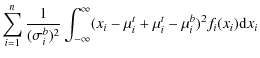
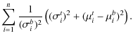
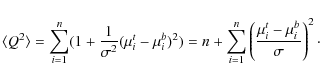
We used the definitions of $\mu_i^t$ and $(\sigma_i^t)^2$ and the property of the probability density function $\int f_i(x_i){\rm d}x_i=1$ . In our case $\sigma_i^t = \sigma_i^b$ holds true without loss of accuracy, and indeed, we simplify $\sigma_i = \sigma$ for all i, that is we assume that the photometric uncertainty is the same for all data points, and argue that this does not pose a problem as long as $\sigma$ is chosen to match the maximum photometric uncertainty. So we can further reduce to

$\begin{displaymath}\langle Q^2\rangle = \sum_{i=1}^n(1+\frac{1}{\sigma^2}(\mu_i^... ...m_{i=1}^n\left(\frac{\mu_i^t - \mu_i^b}{\sigma}\right)^2\cdot \end{displaymath}$

This is the mean of all Q² possibly resulting, when comparing the simulated binary-lens light curve to randomly scattered triple-lens light curve points. It shall be our measure of deviation. Fortunately, we can provide all remaining parameters:

n: is the number of degrees of freedom, equal to the number of compared data points.
$\sigma$: is the assumed standard deviation or photometric uncertainty of observations.
$(\mu_i^t - \mu_i^b)^2$: equals the difference between the two compared light curves squared, which we already use for our least square fit.

$\begin{figure} \par\includegraphics[width=8cm,clip]{13844fgA1.eps} \vspace*{-4mm} \end{figure}$

Figure A.1:

The $\chi ^2$ probability density function plotted for illustration only. For increasing degrees of freedom the central limit theorem takes effect and the curve will very closely resemble a Gaussian distribution. If $P(X\ge\langle Q^2 \rangle) \le 1\%$ , i.e. if the probability P for a $\chi ^2$ -distributed random variable X to be larger or as large as the mean of Q² is less than 0.01, we consider the deviation between the two compared curves to be significant.

Open with DEXTER

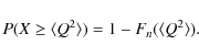
Now we have to decide whether the deviation between our two examined light curves is significant. By taking $\langle Q^2\rangle$ as $\chi ^2$ , one can evaluate the cumulative distribution function $F_n(z) = \int^z_{-\infty} f(x){\rm d}x$ of the $\chi ^2$ -distribution - we relied on the GNU Scientific Library - to find the corresponding probability for any given $\chi ^2$ -distributed random variable X to be as large as or larger than $\langle Q^2\rangle$ ,

$\begin{displaymath}P(X \ge \langle Q^2\rangle) = 1 - F_n(\langle Q^2\rangle). \end{displaymath}$

This probability is just the integral of the $\chi ^2$ probability density function to the right of $\langle Q^2\rangle$ as illustrated in Fig. A.1. If this probability is very small, $\langle Q^2\rangle$ is outside the expected range for a $\chi ^2$ -distributed random variable Q². In that case, Q² is obviously not $\chi ^2$ -distributed with n degrees of freedom, so we must conclude that there is a significant deviation between the triple lens model light curve and the binary-lens model light curve.

We say we have a significant deviation between our two curves, if the mean value $\langle Q^2\rangle$ is so high that the probability Pfor any random variable X being larger or equally large is less than 1%. We interpret this to say, only if the probability for a given triple lens light curve with independent, normally distributed data points to be random fluctuation of the compared binary-lens light curve is less than 1%, we consider it to be principally detectable.

There are two known sources for overestimating the detection rate coming with our method. First, systematic errors are not accounted for. A possible solution could be to add a further term to $\langle Q^2\rangle$ as in $\langle Q_{\rm new}^2 \rangle = \langle Q^2 \rangle - n\left(\frac{\sigma_{\rm sys}}{\sigma}\right)^2$ , where $\sigma_{\rm sys}$ can be assumed to lie in the few percent region for real data. Secondly, we avoid refitting the binary-lens model light curve and always compare to the one we got as best-fit to the exact (simulated) triple-lens model light curve. This overestimation effect vanishes for $n\rightarrow\infty$ and is negligible for a sufficiently large n. The high sampling frequency we use, ensures that the number of data points is always large enough (n > 250 in all cases).

While we cannot exactly quantify the uncertainty of the results, we know that they pose strict upper limits for the lunar detectability in the various scenarios. This knowledge would enable us to infer a tentative census of extrasolar moons, once the first successful microlensing detections have been achieved.

References

Beaulieu, J.-P., Albrow, M., Bennett, D. P., et al. 2006, Nature, 439, 437 [NASA ADS] [CrossRef] [PubMed] [Google Scholar]
Beaulieu, J.-P., Kerins, E., Mao, S., et al. 2008, ESA white paper, submitted [arXiv:0808.0005v1] [Google Scholar]
Benn, C. R. 2001, Earth, Moon and Planets, 85, 61 [Google Scholar]
Bennett, D. P., & Rhie, S. H. 2002, ApJ, 574, 985 [NASA ADS] [CrossRef] [Google Scholar]
Bennett, D. P., Anderson, J., Beaulieu, J.-P., et al. 2009, white paper, submitted [arXiv:0902.3000v1] [Google Scholar]
Bond, I. A., Udalski, A., Jaroszynski, M., et al. 2004, ApJ, 606, L155 [NASA ADS] [CrossRef] [MathSciNet] [Google Scholar]
Bozza, V. 1999, A&A, 348, 311 [NASA ADS] [Google Scholar]
Bozza, V. 2000, A&A, 355, 423 [NASA ADS] [Google Scholar]
Cabrera, J., & Schneider, J. 2007, A&A, 464, 1133 [NASA ADS] [CrossRef] [EDP Sciences] [Google Scholar]
Cassan, A. 2008, A&A, 491, 587 [NASA ADS] [CrossRef] [EDP Sciences] [Google Scholar]
Domingos, R. C., Winter, O. C., & Yokoyama, T. 2006, MNRAS, 373, 1227 [NASA ADS] [CrossRef] [Google Scholar]
Dominik, M., Jørgensen, U. G., Horne, K., et al. 2008, ESA white paper, submitted [arXiv:0808.0004v1] [Google Scholar]
Dong, S., Bond, I. A., Gould, A. P., et al. 2009, ApJ, 698, 1826 [NASA ADS] [CrossRef] [Google Scholar]
Dyson, F. W., Eddington, A. S., & Davidson, C. 1920, R. Soc. London Phil. Trans. Ser. A, 220, 291 [Google Scholar]
Einstein, A. 1916, Ann. Phys., 354, 769 [Google Scholar]
Gaudi, B. S., & Sackett, P. D. 2000, ApJ, 528, 56 [NASA ADS] [CrossRef] [Google Scholar]
Gaudi, B. S., Naber, R. M., & Sackett, P. D. 1998, ApJ, 502, L33 [NASA ADS] [CrossRef] [Google Scholar]
Gaudi, B. S., Bennett, D. P., Udalski, A., Gould, A., et al. 2008, Science, 319, 927 [NASA ADS] [CrossRef] [PubMed] [Google Scholar]
Gaudi, B. S., Beaulieu, J.-P., Bennett, D. P., et al. 2009, white paper, [arXiv:0903.0880v1] [Google Scholar]
Gould, A. P. 2009, in ASP Conf. Ser., ed. K. Z. Stanek, 403, 86 [Google Scholar]
Grundahl, F., Christensen-Dalsgaard, J., Kjeldsen, H., et al. 2009, The Stellar Observations Network Group - the Prototype [arXiv:0908.0436v1] [Google Scholar]
Han, C. 2008, ApJ, 684, 884 [NASA ADS] [CrossRef] [Google Scholar]
Han, C., & Han, W. 2002, ApJ, 580, 490 [NASA ADS] [CrossRef] [Google Scholar]
Holman, M. J., & Murray, N. W. 2005, Science, 307, 1288 [NASA ADS] [CrossRef] [PubMed] [Google Scholar]
Hunter, R. B. 1967, MNRAS, 136, 245 [NASA ADS] [Google Scholar]
Janczak, J., Fukui, A., Dong, S., et al. 2010, ApJ, 711, 731 [NASA ADS] [CrossRef] [Google Scholar]
Kayser, R., Refsdal, S., & Stabell, R. 1986, A&A, 166, 36 [NASA ADS] [Google Scholar]
Kipping, D. M. 2009a, MNRAS, 392, 181 [NASA ADS] [CrossRef] [Google Scholar]
Kipping, D. M. 2009b, MNRAS, 396, 1797 [NASA ADS] [CrossRef] [Google Scholar]
Kipping, D. M., Fossey, S. J., & Campanella, G. 2009, MNRAS, 400, 398 [NASA ADS] [CrossRef] [Google Scholar]
Lewis, K. M., Sackett, P. D., & Mardling, R. A. 2008, ApJ, 685, L153 [NASA ADS] [CrossRef] [Google Scholar]
Liebig, C. 2009, Diploma thesis, Universität Heidelberg [Google Scholar]
Mayor, M., & Queloz, D. 1995, Nature, 378, 355 [NASA ADS] [CrossRef] [Google Scholar]
Muraki, Y., Sumi, T., Abe, F., et al. 1999, Progress of Theoretical Physics Supplement, 133, 233 [Google Scholar]
Paczynski, B. 1996, Ann. Rev. A&A, 34, 419 [CrossRef] [Google Scholar]
Réfrégier, A., Amara, A., Kitching, T. D., et al. 2010, Euclid Imaging Consortium Science Book [arXiv:1001.0061v1] [Google Scholar]
Rhie, S. H. 1997, ApJ, 484, 63 [NASA ADS] [CrossRef] [Google Scholar]
Rhie, S. H. 2002, How Cumbersome is a Tenth Order Polynomial? The Case of Gravitational Triple Lens Equation [arXiv:astro-ph/0202294v1] [Google Scholar]
Sartoretti, P., & Schneider, J. 1999, A&AS, 134, 553 [NASA ADS] [CrossRef] [EDP Sciences] [Google Scholar]
Scharf, C. A. 2006, ApJ, 648, 1196 [NASA ADS] [CrossRef] [Google Scholar]
Schneider, P., & Weiß, A. 1986, A&A, 164, 237 [NASA ADS] [Google Scholar]
Schneider, P., Kochanek, C. S., & Wambsganss, J. 2006, Gravitational Lensing: Strong, Weak and Micro, Saas-Fee Advanced Courses 33 (Berlin, Heidelberg: Springer-Verlag) [Google Scholar]
Southworth, J., Hinse, T. C., Jørgensen, U. G., et al. 2009, MNRAS, 396, 1023 [NASA ADS] [CrossRef] [Google Scholar]
Udalski, A., Szymanski, M., Ka▯uzny, J., Kubiak, M., & Mateo, M. 1992, Acta Astron., 42, 253 [NASA ADS] [Google Scholar]
Wambsganss, J. 1990, Ph.D. Thesis, Ludwig-Maximilians-Universität München [Google Scholar]
Wambsganss, J. 1997, MNRAS, 284, 172 [NASA ADS] [Google Scholar]
Wambsganss, J. 1999, J. Comput. Appl. Math., 109, 353 [NASA ADS] [CrossRef] [Google Scholar]
Williams, D. M., & Knacke, R. F. 2004, Astrobiology, 4, 400 [NASA ADS] [CrossRef] [PubMed] [Google Scholar]
Witt, H. J. 1990, A&A, 236, 311 [NASA ADS] [Google Scholar]

Footnotes

... detected

exoplanet.eu

... unbiased

I.e. independent of lunar features, but required to pass close to or through the planetary caustic.

... Euclid

http://sci.esa.int/euclid

... distribution

We recall the definitions of mean and variance. For the random variable X with probability density function f(x), they are in general

$\displaystyle \mu$	=	$\displaystyle \int_{-\infty}^{\infty} x\;f(x)\; {\rm d}x = \langle X \rangle \quad {\rm and}$
$\displaystyle \sigma^2$	=	$\displaystyle \int_{-\infty}^{\infty} (x-\mu)^2\;f(x)\;{\rm d} x = \langle (X-\mu)^2 \rangle,$

where we also introduce the notation $\langle X \rangle$ for the expectation value of X.

... $\chi ^2$ -distributed

The $\chi ^2$ -distribution can be applied to the sum of n independent, normally distributed random variables Z_i with the mean $\mu_i=0$ and the standard deviation $\sigma_i=1$ for all i,

$\begin{displaymath}\chi^2 \sim \sum_{i=1}^n Z_i^2. \end{displaymath}$

See any standard book with an introduction to calculus of probability.

... Library

http://www.gnu.org/software/gsl/

All Tables

Table 1: Parameter values of our standard scenario.

Table 2: Detectability of the third mass in the magnification pattern of Fig. 5, for different assumed photometric uncertainties.

Table 3: Detectability of the moon in our standard scenario as a function of assumed photometric uncertainty.

Table 4: Detectability of the moon as a function of the planet-moon separation for our standard scenario.

Table 5: Detectability of the moon depending on moon-planet mass ratio.

Table 6: Dependence of lunar detectability as a function of the planet-star mass ratio, all other parameters as in our standard scenario.

Table 7: Detectability of the moon depending on the sampling rate of the simulated light curves.

Table 8: Detectability of the moon depending on the size of the source star, all other parameters as in our standard scenario.

All Figures

$\begin{figure} \par\includegraphics[width=8.8cm,clip]{13844fg01.eps} \end{figure}$	Figure 1: Geometry of our triple-lens scenario, not to scale. Five parameters have to be fixed: the mass ratios $q_{\rm PS} = M_{\rm Planet}/M_{\rm Star}$ and $q_{\rm MP} = M_{\rm Moon}/M_{\rm Planet}$ , the angular separations in the lens plane $\theta _{\rm PS}$ and $\theta _{\rm MP}$ and the position angle of the moon $\phi$ . These parameters define uniquely the relative projected positions of the three bodies.
Open with DEXTER
In the text

$\begin{figure} \par\includegraphics[height=22cm,width=16.5cm,clip]{13844fg02.eps} \end{figure}$	Figure 2: Details of the analysed triple-lens magnification maps for an example mass/separation scenario with $q_{\rm PS}= 10^{-3}$ , $q_{\rm MP}=10^{-2}$ , $\theta_{\rm PS}=1.3~\ensuremath{\theta_{E}}$ and $\theta_{\rm MP}=1.0~\ensuremath{\theta_{E}} ^P$ (the standard scenario as summarised in Table 1), showing the caustic configurations for twelve different lunar positions completing a full circular orbit in steps of 30 $\hbox {$^\circ $ }$ . The relative positions of star, planet and moon are sketched in the lower left of each panel (not to scale). The side lengths of the individual frames are $0.1~\ensuremath{\theta_{E}}$ . A darker shade of grey corresponds to a higher magnification. The straight black lines mark source trajectories, the resulting light curves are displayed in Fig. 3.
Open with DEXTER
In the text

$\begin{figure} \par\includegraphics[height=22cm,width=16.5cm,clip]{13844fg03.eps} \end{figure}$	Figure 3: Sample of triple-lens light curves corresponding to the source trajectories depicted in Fig. 2. The solid light curves were extracted with an assumed solar source size, $R_{\rm Source} = R{_{\hbox {$\odot $ }}}$ ; the thin, dashed lines show the same light curves with $R_{\rm Source} = 3~R{_{\hbox{$\odot$ }}}$ . The magnification scale is given in negative magnitude difference ( $-\Delta$ mag), i.e. the unmagnified baseline flux of the source is 0. The time scale in units of the Einstein time t_E, assuming a uniform relative motion of source and lens.
Open with DEXTER
In the text

$\begin{figure} \par\includegraphics[width=8.5cm,clip]{13844fg04.eps} \end{figure}$	Figure 4: Magnification pattern displaying the planetary caustic of a triple-lens system with mass ratios $q_{\rm PS}= 10^{-3}$ and $q_{\rm MP}=10^{-2}$ , corresponding, e.g., to an M-dwarf, a Saturn-mass planet and an Earth-mass satellite of that planet. Darker shades correspond to areas of higher magnification. The third body shows its influence as the small perturbation on the bottom cusp of the planetary caustic. The position angle of the moon is $\phi =90\hbox {$^\circ $ }$ , i.e. in the orientation of this map the moon is located above the planet. The complete set of parameters is given in Table 1. The side length of the pattern is $0.1~\theta_{E}$ in stellar Einstein radii. A source with radius $R_{\hbox {$\odot $ }}$ (2 $R_{\hbox {$\odot $ }}$ , 3 $R_{\hbox {$\odot $ }}$ , 5 $R_{\hbox {$\odot $ }}$ ) is indicated as a black disc (dashed circles) in the lower left. Taking the straight line that cuts the lunar perturbation of the caustic as the source trajectory of a solar sized source results in the light curve shown in Fig. 6 (solid line). Depending on the assumed source size, different light curves are obtained, see also Figs. 9a to c.
Open with DEXTER
In the text

$\begin{figure} \par\includegraphics[width=8.5cm,clip]{13844fg05.eps} \end{figure}$	Figure 5: Illustration of how the magnification pattern of a given star-planet-moon configuration is evaluated. In order to have an unbiased statistical sample, the source trajectories are chosen independently of the lunar caustic features, though all light curves are required to pass through or close to the planetary caustic. This is realised through generating a grid of source trajectories that is only oriented at the planetary caustic. In the actual evaluation a 10 times denser grid than shown here was used. The magnification map has to be substantially larger than the caustic to ensure an adequate baseline for the light curve fitting. The side length of this pattern is $0.3~\theta_{E}$ , the position angle of the moon $\phi =90\hbox {$^\circ $ }$ , all other parameters are chosen as listed in Table 1. Source sizes of 1 $R_{\hbox {$\odot $ }}$ , 2 $R_{\hbox {$\odot $ }}$ , 3 $R_{\hbox {$\odot $ }}$ , and 5 $R_{\hbox {$\odot $ }}$ are indicated in the lower left.
Open with DEXTER
In the text

$\begin{figure} \par\includegraphics[width=8.5cm,clip]{13844fg06.eps} \vspace*{-3mm} \end{figure}$	Figure 6: Triple-lens light curve (solid line) extracted from the magnification pattern in Fig. 4, compared with a light curve extracted from the corresponding binary-lens magnification map (dashed line), with no third body and the planet mass increased by the previous moon mass. The difference of the two light curves is plotted as the dotted line. The central peak of the triple-lens light curve is caused by lunar caustic perturbations, that cannot easily be reproduced with a binary lens. In a), identical source trajectory parameters are used to extract the binary-lens light curve and large residuals remain that can be avoided with a different source trajectory. In b), the best-fit binary-lens light curve is shown (dashed) in comparison with the triple-lens light curve (solid). Here, the residuals can be attributed to the moon. If the deviation is significant, the moon is detectable in the triple-lens light curve. A source with solar radius at a distance of 8 kpc is assumed.
Open with DEXTER
In the text

$\begin{figure} \par\mbox{\subfigure[$q_{\rm MP}=10^{-3}$ ]{\includegraphics[widt... ... ]{\includegraphics[width=3cm]{13844fg07c.eps} }}\vspace*{-3.5mm} \end{figure}$	Figure 7: Caustic topology with different lunar mass ratios. From left to right, the lunar mass ratio increases from $q_{\rm MP} = 10^{-3}$ to 10^-1. The side length of the displayed patterns is $0.05~\ensuremath{\theta_{E}}$ . All other parameters as given in Table 1, in particular $q_{\rm PS}= 10^{-3}$ and $\theta_{\rm MP}=1.0~\ensuremath{\theta_{E}} ^P$ . Source sizes of $1~R{_{\hbox{$\odot$ }}}$ to $5~R\ensuremath{_{\hbox{$\odot$ }}}$ are indicated in the lower left.
Open with DEXTER
In the text

$\begin{figure} \par\mbox{\subfigure[$\theta_{\rm MP}=0.8~\ensuremath{\theta_{E}}... ... ]{ \includegraphics[width=3cm]{13844fg08c.eps} } }\vspace*{-4mm} \end{figure}$	Figure 8: Magnification patterns with side lengths of $0.05~\ensuremath{\theta_{E}}$ showing the lunar perturbation of the planetary caustic for increasing angular separations of moon and planet of $\theta_{\rm MP}= 0.8~\ensuremath{\theta_{E}} ^P, 1.0~\ensuremath{\theta_{E}} ^P, 1.2~\ensuremath{\theta_{E}} ^P$ , while all other parameters are as in Table 1. The topology of interaction varies with the angular separation. Source sizes of $1~R\ensuremath{_{\hbox{$\odot$ }}}$ to $5~R\ensuremath{_{\hbox{$\odot$ }}}$ are indicated in the lower left.
Open with DEXTER
In the text

$\begin{figure} \par\includegraphics[width=8.5cm,clip]{13844fg9.eps} \vspace*{-2.5mm} \end{figure}$	Figure 9: Illustration of the increasing source radius, compare Fig. 6b: a) $R_{\rm source} = 2_{\hbox {$\odot $ }}$ , b) $3~R_{\hbox{$\odot$ }}$ , and c) $5~R_{\hbox{$\odot$ }}$ , all other parameters as given in Table 1. The triple-lens light curve (solid) is obtained from the magnification pattern in Fig. 4, the best-fit binary-lens light curve (dashed) from the corresponding magnification pattern without a moon. The difference between the two curves is plotted as a dotted line.
Open with DEXTER
In the text

$\begin{figure} \par\includegraphics[width=16cm,clip]{13844fg10.eps}\vspace*{-2mm} \end{figure}$	Figure 10: Visualisation of the approximate lunar resonance zone (dark-grey ring), where planetary and lunar caustic overlap and interact. Also depicted is the planet lensing zone (light grey), which is the area of planet positions for which the planetary caustic(s) lie within the stellar Einstein radius. Distances and caustic inset are to scale. The physical scale depends not only on the masses of the lensing bodies, but also on the distances to the lens system and the background star. In our adopted standard scenario, cf. Table 1, the Einstein radius $\theta _E$ corresponds to 1.9 AU in the lens plane. This places the planet at a projected orbit radius of 2.5 AU, whereas the moon's orbit has a radius of 0.06 AU (corresponding to one planetary Einstein radius). The lunar resonance zone covers lunar orbit radii from 0.04 AU to 0.18 AU.
Open with DEXTER
In the text

$\begin{figure} \par\includegraphics[width=8cm,clip]{13844fgA1.eps} \vspace*{-4mm} \end{figure}$	Figure A.1: The $\chi ^2$ probability density function plotted for illustration only. For increasing degrees of freedom the central limit theorem takes effect and the curve will very closely resemble a Gaussian distribution. If $P(X\ge\langle Q^2 \rangle) \le 1\%$ , i.e. if the probability P for a $\chi ^2$ -distributed random variable X to be larger or as large as the mean of Q² is less than 0.01, we consider the deviation between the two compared curves to be significant.
Open with DEXTER
In the text

Current usage metrics show cumulative count of Article Views (full-text article views including HTML views, PDF and ePub downloads, according to the available data) and Abstracts Views on Vision4Press platform.

Data correspond to usage on the plateform after 2015. The current usage metrics is available 48-96 hours after online publication and is updated daily on week days.

Initial download of the metrics may take a while.

[1] Beaulieu, J.-P., Albrow, M., Bennett, D. P., et al. 2006, Nature, 439, 437 [NASA ADS] [CrossRef] [PubMed] [Google Scholar]

[2] Beaulieu, J.-P., Kerins, E., Mao, S., et al. 2008, ESA white paper, submitted [arXiv:0808.0005v1] [Google Scholar]

[3] Benn, C. R. 2001, Earth, Moon and Planets, 85, 61 [Google Scholar]

[4] Bennett, D. P., & Rhie, S. H. 2002, ApJ, 574, 985 [NASA ADS] [CrossRef] [Google Scholar]

[5] Bennett, D. P., Anderson, J., Beaulieu, J.-P., et al. 2009, white paper, submitted [arXiv:0902.3000v1] [Google Scholar]

[6] Bond, I. A., Udalski, A., Jaroszynski, M., et al. 2004, ApJ, 606, L155 [NASA ADS] [CrossRef] [MathSciNet] [Google Scholar]

[7] Bozza, V. 1999, A&A, 348, 311 [NASA ADS] [Google Scholar]

[8] Bozza, V. 2000, A&A, 355, 423 [NASA ADS] [Google Scholar]

[9] Cabrera, J., & Schneider, J. 2007, A&A, 464, 1133 [NASA ADS] [CrossRef] [EDP Sciences] [Google Scholar]

[10] Cassan, A. 2008, A&A, 491, 587 [NASA ADS] [CrossRef] [EDP Sciences] [Google Scholar]

[11] Domingos, R. C., Winter, O. C., & Yokoyama, T. 2006, MNRAS, 373, 1227 [NASA ADS] [CrossRef] [Google Scholar]

[12] Dominik, M., Jørgensen, U. G., Horne, K., et al. 2008, ESA white paper, submitted [arXiv:0808.0004v1] [Google Scholar]

[13] Dong, S., Bond, I. A., Gould, A. P., et al. 2009, ApJ, 698, 1826 [NASA ADS] [CrossRef] [Google Scholar]

[14] Dyson, F. W., Eddington, A. S., & Davidson, C. 1920, R. Soc. London Phil. Trans. Ser. A, 220, 291 [Google Scholar]

[15] Einstein, A. 1916, Ann. Phys., 354, 769 [Google Scholar]

[16] Gaudi, B. S., & Sackett, P. D. 2000, ApJ, 528, 56 [NASA ADS] [CrossRef] [Google Scholar]

[17] Gaudi, B. S., Naber, R. M., & Sackett, P. D. 1998, ApJ, 502, L33 [NASA ADS] [CrossRef] [Google Scholar]

[18] Gaudi, B. S., Bennett, D. P., Udalski, A., Gould, A., et al. 2008, Science, 319, 927 [NASA ADS] [CrossRef] [PubMed] [Google Scholar]

[19] Gaudi, B. S., Beaulieu, J.-P., Bennett, D. P., et al. 2009, white paper, [arXiv:0903.0880v1] [Google Scholar]

[20] Gould, A. P. 2009, in ASP Conf. Ser., ed. K. Z. Stanek, 403, 86 [Google Scholar]

[21] Grundahl, F., Christensen-Dalsgaard, J., Kjeldsen, H., et al. 2009, The Stellar Observations Network Group - the Prototype [arXiv:0908.0436v1] [Google Scholar]

[22] Han, C. 2008, ApJ, 684, 884 [NASA ADS] [CrossRef] [Google Scholar]

[23] Han, C., & Han, W. 2002, ApJ, 580, 490 [NASA ADS] [CrossRef] [Google Scholar]

[24] Holman, M. J., & Murray, N. W. 2005, Science, 307, 1288 [NASA ADS] [CrossRef] [PubMed] [Google Scholar]

[25] Hunter, R. B. 1967, MNRAS, 136, 245 [NASA ADS] [Google Scholar]

[26] Janczak, J., Fukui, A., Dong, S., et al. 2010, ApJ, 711, 731 [NASA ADS] [CrossRef] [Google Scholar]

[27] Kayser, R., Refsdal, S., & Stabell, R. 1986, A&A, 166, 36 [NASA ADS] [Google Scholar]

[28] Kipping, D. M. 2009a, MNRAS, 392, 181 [NASA ADS] [CrossRef] [Google Scholar]

[29] Kipping, D. M. 2009b, MNRAS, 396, 1797 [NASA ADS] [CrossRef] [Google Scholar]

[30] Kipping, D. M., Fossey, S. J., & Campanella, G. 2009, MNRAS, 400, 398 [NASA ADS] [CrossRef] [Google Scholar]

[31] Lewis, K. M., Sackett, P. D., & Mardling, R. A. 2008, ApJ, 685, L153 [NASA ADS] [CrossRef] [Google Scholar]

[32] Liebig, C. 2009, Diploma thesis, Universität Heidelberg [Google Scholar]

[33] Mayor, M., & Queloz, D. 1995, Nature, 378, 355 [NASA ADS] [CrossRef] [Google Scholar]

[34] Muraki, Y., Sumi, T., Abe, F., et al. 1999, Progress of Theoretical Physics Supplement, 133, 233 [Google Scholar]

[35] Paczynski, B. 1996, Ann. Rev. A&A, 34, 419 [CrossRef] [Google Scholar]

[36] Réfrégier, A., Amara, A., Kitching, T. D., et al. 2010, Euclid Imaging Consortium Science Book [arXiv:1001.0061v1] [Google Scholar]

[37] Rhie, S. H. 1997, ApJ, 484, 63 [NASA ADS] [CrossRef] [Google Scholar]

[38] Rhie, S. H. 2002, How Cumbersome is a Tenth Order Polynomial? The Case of Gravitational Triple Lens Equation [arXiv:astro-ph/0202294v1] [Google Scholar]

[39] Sartoretti, P., & Schneider, J. 1999, A&AS, 134, 553 [NASA ADS] [CrossRef] [EDP Sciences] [Google Scholar]

[40] Scharf, C. A. 2006, ApJ, 648, 1196 [NASA ADS] [CrossRef] [Google Scholar]

[41] Schneider, P., & Weiß, A. 1986, A&A, 164, 237 [NASA ADS] [Google Scholar]

[42] Schneider, P., Kochanek, C. S., & Wambsganss, J. 2006, Gravitational Lensing: Strong, Weak and Micro, Saas-Fee Advanced Courses 33 (Berlin, Heidelberg: Springer-Verlag) [Google Scholar]

[43] Southworth, J., Hinse, T. C., Jørgensen, U. G., et al. 2009, MNRAS, 396, 1023 [NASA ADS] [CrossRef] [Google Scholar]

[44] Udalski, A., Szymanski, M., Ka▯uzny, J., Kubiak, M., & Mateo, M. 1992, Acta Astron., 42, 253 [NASA ADS] [Google Scholar]

[45] Wambsganss, J. 1990, Ph.D. Thesis, Ludwig-Maximilians-Universität München [Google Scholar]

[46] Wambsganss, J. 1997, MNRAS, 284, 172 [NASA ADS] [Google Scholar]

[47] Wambsganss, J. 1999, J. Comput. Appl. Math., 109, 353 [NASA ADS] [CrossRef] [Google Scholar]

[48] Williams, D. M., & Knacke, R. F. 2004, Astrobiology, 4, 400 [NASA ADS] [CrossRef] [PubMed] [Google Scholar]

[49] Witt, H. J. 1990, A&A, 236, 311 [NASA ADS] [Google Scholar]