| Issue |
A&A
Volume 512, March-April 2010
|
|
|---|---|---|
| Article Number | A49 | |
| Number of page(s) | 13 | |
| Section | Extragalactic astronomy | |
| DOI | https://doi.org/10.1051/0004-6361/200913072 | |
| Published online | 31 March 2010 | |
INTEGRAL hard X-ray spectra of the cosmic X-ray background and Galactic ridge emission
M. Türler1,2 - M. Chernyakova3 - T. J.-L. Courvoisier1,2 - P. Lubinski1,4 - A. Neronov1,2 - N. Produit1,2 - R. Walter1,2
1 - ISDC Data Centre for Astrophysics, ch. d'Ecogia 16, 1290 Versoix, Switzerland
2 - Geneva Observatory, University of Geneva, ch. des Maillettes 51, 1290 Sauverny, Switzerland
3 - Dublin Institute for Advanced Studies, 31 Fitzwilliam Place, Dublin 2, Ireland
4 - Nicolaus Copernicus Astronomical Center, Bartycka 18, 00-716 Warszawa, Poland
Received 5 August 2009 / Accepted 4 January 2010
Abstract
Aims. We derive the spectra of the cosmic X-ray background (CXB) and of the Galactic ridge X-ray emission (GRXE) in the ![]() 20-200 keV range from the data of the IBIS instrument aboard the INTEGRAL satellite obtained during the four dedicated Earth-occultation observations in early 2006.
20-200 keV range from the data of the IBIS instrument aboard the INTEGRAL satellite obtained during the four dedicated Earth-occultation observations in early 2006.
Methods. We analyze the modulation of the IBIS/ISGRI detector
counts induced by the passage of the Earth through the field of view of
the instrument. Unlike previous studies, we do not fix the spectral
shape of the various contributions, but model instead their spatial
distribution and derive for each of them the expected modulation of the
detector counts. The spectra of the diffuse emission components are
obtained by fitting the normalizations of the model lightcurves to the
observed modulation in different energy bins. Because of degeneracy, we
guide the fits with a realistic choice of the input parameters and a
constraint for spectral smoothness.
Results. The obtained CXB spectrum is consistent with the historic HEAO-1 results and falls slightly below the spectrum derived with Swift/BAT.
A 10% higher normalization of the CXB cannot be completely excluded,
but it would imply an unrealistically high albedo of the Earth. The
derived spectrum of the GRXE confirms the presence of a minimum around
80 keV with improved statistics and yields an estimate of ![]() 0.6
0.6
![]() for the average mass of white dwarfs in the Galaxy. The analysis also
provides updated normalizations for the spectra of the Earth's albedo
and the cosmic-ray induced atmospheric emission.
for the average mass of white dwarfs in the Galaxy. The analysis also
provides updated normalizations for the spectra of the Earth's albedo
and the cosmic-ray induced atmospheric emission.
Conclusions. This study demonstrates the potential of INTEGRAL
Earth-occultation observations to derive the hard X-ray spectra of
three fundamental components: the CXB, the GRXE and the Earth emission.
Further observations would be extremely valuable to confirm our results
with improved statistics.
Key words: earth - Galaxy: disk - galaxies: active - diffuse radiation - X-rays: diffuse background - X-rays: general
1 Introduction
Although the cosmic X-ray background (CXB) was discovered before the cosmic microwave background (Giacconi et al. 1962), it is known in much less detail and its spectral shape and normalization are still subjects of debate. This diffuse emission is thought to be mainly due to unresolved active galactic nuclei (AGN) extending to cosmological distances with a contribution from type Ia supernovae in the low-energy gamma-rays (Zdziarski 1996). Evidence for the AGN origin of the CXB at energies below 10 keV comes from various X-ray mirror telescopes - in particular Chandra and XMM-Newton - that were able to resolve up to 80% of the diffuse emission into point sources (e.g. Gilli et al. 2007; Brandt & Hasinger 2005). The amount of resolved sources decreases rapidly with energy though so that only 2.5% of the diffuse background is resolved by the deepest survey yet in the 20-60 keV range, at the peak of the CXB emission (Paltani et al. 2008). The characterization of the actual spectral shape and normalization around this emission bump is crucial to estimate the fraction of heavily absorbed Compton-thick AGN thought to contribute significantly in this hard X-ray spectral range (Ueda et al. 2003; Sazonov et al. 2008; Treister et al. 2009; Gilli et al. 2007).
The High Energy Astronomical Observatory 1 (HEAO-1) is hitherto the only satellite which had a dedicated mechanism to disentangle the CXB from the instrumental background. By using a movable CsI crystal with a thickness of 5 cm to cover part of the field of view (FoV), the HEAO-1 observations of the mid-1970s are still the most accurate and reliable measurements of the CXB spectral shape in the hard X-rays (Gruber et al. 1999; Marshall et al. 1980; Kinzer et al. 1997). Without such a masking mechanism in recent space missions, a practical way to study this diffuse hard X-ray emission is to use the Earth as a screen occulting part of the background sky. For pointing satellites in low orbits around the Earth, our planet often crosses part of the field of view during normal operations. Such events can be analyzed in detail to evaluate the CXB spectrum. This was done by Frontera et al. (2007) for the BeppoSAX mission and by Ajello et al. (2008) for the data of the Burst Alert Telescope (BAT) aboard the Swift spacecraft.
![\begin{figure}
\par\includegraphics[width=6cm]{13072f1a.eps}\includegraphics[width=6cm]{13072f1b.eps}
\end{figure}](/articles/aa/full_html/2010/04/aa13072-09/img9.png)
|
Figure 1:
Model IBIS/ISGRI images of the sky with ( right) and without ( left) instrumental vignetting effects (see Fig. 2). They show the geometry and relative intensity (on a logarithmic scale from dark and blue to
red and bright areas) of the various components during the first EO at
IJD = 2216.04 as derived for channel 3 ( |
| Open with DEXTER | |
With its eccentric three-days orbit, the INTEGRAL satellite (Winkler et al. 2003) is close to the Earth only during the perigee passage when the instruments are not operating because of excessive background in the radiation belts. In order to study the X-ray background, a series of four dedicated observations were performed in January and February 2006. The Earth was allowed to pass through the FoV of the instruments shortly after radiation-belt exit while the spacecraft was aimed to point towards a fixed position in the sky. Churazov et al. (2007) described these observations by all four instruments aboard INTEGRAL in great detail and studied how the passage of the Earth modulates the detector counts by occulting part of the CXB.
The difficulty of using the Earth to shield the CXB comes from the fact that the Earth is not dark in the hard X-rays. The emission from the Earth in the 20-200 keV range consists of two major contributions: the reflection of the CXB by the atmosphere and its Compton emission under the bombardment by cosmic rays (CR). Disentangling the CXB occultation from the Earth emission is challenging. Churazov et al. (2007) assumed the spectral shape of the CXB and of the two Earth emission components and fitted their normalizations to the observed amplitude of the Earth modulation in the data. The studies of the BeppoSAX/PDS measurements (Frontera et al. 2007) and the Swift/BAT observations (Ajello et al. 2008) also relied on a priori assumptions on the spectral shape of the CXB and the Earth emission.
We present here a completely different approach for the analysis of the same INTEGRAL observations as were used by Churazov et al. (2007), but only focusing on the data of the IBIS/ISGRI instrument (Ubertini et al. 2003). Instead of fixing the spectral shapes of the CXB and the Earth emission components, we aim to derive them based on a detailed modeling of the spatial distribution of these components and of all instrumental effects. If the Earth surface brightness differs significantly from the uniform CXB occultation, it is possible to disentangle these components based on the recorded modulation when the Earth is crossing the FoV. This has the potential to simultaneously derive the spectral shape of the CXB and of the Earth emission from the observations.
Another difficulty of the analysis is the presence of the Galactic plane in the border of the wide FoV of IBIS (see Fig. 1). An empty extragalactic field would have been ideal to study the CXB, but this was not possible due to various scheduling constraints. This complication is however an opportunity to study in addition the diffuse Galactic ridge X-ray emission (GRXE) (e.g. Revnivtsev et al. 2006; Bouchet et al. 2008; Krivonos et al. 2007), which is also occulted by the passage of the Earth.
The observational material and the analysis method are described in
Sects. 2 and 3, respectively. We present the obtained spectra in
Sect. 4 and discuss them in comparison to previous results in
Sect. 5, before concluding in Sect. 6. Unless
otherwise stated, the quoted errors are 1-![]() uncertainties, i.e. at the
68% confidence level (CL).
uncertainties, i.e. at the
68% confidence level (CL).
2 Data
The data used here are the four Earth-occultation observations (EOs) conducted
by INTEGRAL in January and February 2006 at the start of satellite
revolutions number 401, 404, 405 and 406. We refer the reader to the detailed
description of these observations in Churazov et al. (2007). We focus our analysis on the data of the IBIS/ISGRI gamma-ray imager that is best suited to study the
emission in the ![]() 20-200 keV range.
20-200 keV range.
Our work is based on the analysis of the modulation in full detector lightcurves induced by the passage of the Earth through the FoV. These lightcurves are obtained with the latest version of the ii_light executable that will be included in a forthcoming release of the Off-line Scientific Analysis (OSA) software package provided by the INTEGRAL Science Data Centre (ISDC, Courvoisier et al. 2003). They are corrected for instrumental dead time and the effect of dead and noisy pixels, which amount to typically 5% of all ISGRI pixels. For each of the four similar observations, we extracted detector lightcurves with a time binning of 300 s in a series of 16 energy bins (see Table 2), carefully chosen to isolate instrumental emission features, in particular the broad lines at 26 and 31 keV from CdTe and the narrow lines at 59 keV from W, 75-77 keV from Pb and 82-84 keV from Bi (Terrier et al. 2003).
The detector lightcurves originally expressed in units of count cm-2 s-1 were
multiplied by 0.5 (
![]() cm)2 = 1310.72 cm2,
which is the
area of the detector assumed by the standard ISGRI ancillary response
file
(ARF), describing the energy dependence of the effective area of the
instrument. The factor 0.5 refers to the fraction of open coded
mask elements, and 0.4 cm is the size of the
cm)2 = 1310.72 cm2,
which is the
area of the detector assumed by the standard ISGRI ancillary response
file
(ARF), describing the energy dependence of the effective area of the
instrument. The factor 0.5 refers to the fraction of open coded
mask elements, and 0.4 cm is the size of the
![]() ISGRI detector elements. Apart from this change of unit to have full
detector lightcurves, the only other manipulation of
the data was a cleaning of the lightcurves. This was done by removing
points
with uncertainties of more than twice the average uncertainty and by
iteratively removing a few isolated outstanding points lying more than 3
ISGRI detector elements. Apart from this change of unit to have full
detector lightcurves, the only other manipulation of
the data was a cleaning of the lightcurves. This was done by removing
points
with uncertainties of more than twice the average uncertainty and by
iteratively removing a few isolated outstanding points lying more than 3![]() away from the smoothed lightcurve with a smoothing window of 30 min (i.e. 6 time bins).
away from the smoothed lightcurve with a smoothing window of 30 min (i.e. 6 time bins).
Table 1: List of point sources detected in at least one of the four EOs.
In order to subtract from the lightcurves the contribution of point sources in
the FoV, we performed an image analysis separately for the four Earth
observations. This was possible since the drift of the satellite was moderate
despite the absence of star trackers during the pointings. The image analysis
was done in a standard way with the default background maps of OSA 7.0. We
searched for all sources previously detected by ISGRI including the new source
IGR J17062-6143 already reported by Churazov et al. (2007). We then selected all sources that were detected with a significance of more than 2![]() in the
22-60 keV band. We chose this low significance threshold to minimize the
contribution of the known point sources to the GRXE and the CXB. Sources with
even less significance are more likely to be spurious and their global
contribution will mostly cancel out with fake negative sources. We tested
both a simple powerlaw and a bremsstrahlung model to fit the data. We found that
for most sources the bremsstrahlung model gives a better phenomenological
description of the data than a powerlaw because many sources have a convex
spectral shape in this energy range. The fluxes derived for the brightest
(>3
in the
22-60 keV band. We chose this low significance threshold to minimize the
contribution of the known point sources to the GRXE and the CXB. Sources with
even less significance are more likely to be spurious and their global
contribution will mostly cancel out with fake negative sources. We tested
both a simple powerlaw and a bremsstrahlung model to fit the data. We found that
for most sources the bremsstrahlung model gives a better phenomenological
description of the data than a powerlaw because many sources have a convex
spectral shape in this energy range. The fluxes derived for the brightest
(>3![]() )
sources in our sample are listed in Table 1.
)
sources in our sample are listed in Table 1.
3 Method
The detector lightcurves described above were modulated by the passage of the Earth through the FoV of IBIS. Our approach was to model these observations in detail to derive the expected modulation of the detector counts for each emission component on the sky. This resulted in a series of model lightcurves in different energy bins for each emission component and each of the four EOs. We then fitted the normalizations of these model lightcurves to the observed detector counts to derive the actual contribution of the diffuse emission components.
This method requires the knowledge of the spacecraft position and attitude with respect to the Earth and to the background sky at any time, a description of the spatial distribution on the sky of the various emission components and also an accurate description of the IBIS/ISGRI instrumental characteristics. These aspects are described in the three subsections below. The generation of the model lightcurves is described in Sect. 3.4, whereas the actual spectral fitting procedure is the subject of Sect. 3.5.
Table 2: Numerical values of the obtained spectra shown in Fig. 6.
3.1 Satellite position and attitude
To construct the images of the sky corresponding to each of the four Earth
observations as illustrated in Fig. 1, we needed to know the exact
attitude of the satellite and its distance to the Earth at any time. This
information can be extracted from auxiliary files provided by the mission
operation centre (MOC) in Darmstadt. It was used to compute the position of the
Earth center, the position of the geographic and magnetic poles, and the
apparent radius of the Earth as a function of time, all expressed in
degrees, using the IBIS/ISGRI instrument coordinates (Y,Z).
The
spacecraft was close enough to the Earth at the beginning of the
observation for the planet's sphericity to slightly affect its apparent
radius. This was
properly taken into account, as well as the ![]() 100 km of obscuring
atmosphere in the hard X-rays mentioned by Churazov et al. (2007). The magnetic pole in the Northern hemisphere is set to its 2005 position of 82.7
100 km of obscuring
atmosphere in the hard X-rays mentioned by Churazov et al. (2007). The magnetic pole in the Northern hemisphere is set to its 2005 position of 82.7![]() N,
114.4
N,
114.4![]() W.
W.
3.2 Spatial distribution of components
Although we were only interested in the temporal modulation of counts on the full detector area, we needed a sufficiently precise description of the spatial distribution of the emission components. We chose to define all of them by analytical functions that are described below and are illustrated in Fig. 1.
The simplest component is the CXB that we assumed to be uniform on the sky.
Although there is evidence that the CXB has some large-scale intensity
variations (e.g. Boughn et al. 2002; Revnivtsev et al. 2008), they are small in amplitude
(![]() 2%) and it would be very difficult to evaluate and account for a
possible non-uniformity so close to the Galactic bulge.
2%) and it would be very difficult to evaluate and account for a
possible non-uniformity so close to the Galactic bulge.
The GRXE was modeled with two perpendicular Lorentzian functions aligned with
the Galactic coordinates. The full-width at half maximum (FWHM) of the
Lorentzians are of
![]() (Krivonos et al. 2007, Fig. 7) and
(Krivonos et al. 2007, Fig. 7) and ![]() (Revnivtsev et al. 2006, Fig. 5) respectively along the Galactic longitude, l, and
latitude, b. The Lorentzian's maximum are at the Galactic center with a slight latitude displacement of
(Revnivtsev et al. 2006, Fig. 5) respectively along the Galactic longitude, l, and
latitude, b. The Lorentzian's maximum are at the Galactic center with a slight latitude displacement of
![]() as measured by Revnivtsev et al. (2006). As
shown by Krivonos et al. (2007), this distribution matches well the COBE/DIRBE map at 4.9
as measured by Revnivtsev et al. (2006). As
shown by Krivonos et al. (2007), this distribution matches well the COBE/DIRBE map at 4.9 ![]() m, which was used by Bouchet et al. (2008) as a template for the GRXE below 120 keV.
m, which was used by Bouchet et al. (2008) as a template for the GRXE below 120 keV.
We took special care to define the spatial distribution of the Earth's emission. There are two distinct components to be taken into account: the CXB reflection by the Earth (Churazov et al. 2008) and the CR-induced atmospheric emission (Sazonov et al. 2007). The authors of these studies performed Monte-Carlo simulations to derive both the spectrum and the surface brightness of the Earth emission. We used the latter results as a precise determination of the expected image of the Earth at hard X-rays.
Churazov et al. (2008) found that the X-ray albedo of the Earth is limb-darkened
at lower energies and limb-brightened at higher energies. At energies below
![]() 100 keV - where this component dominates the Earth emission - the
emission is found to be limb-darkened, but slightly less than for a sphere
emitting black-body radiation. Such an object would have a linear dependence of
the flux with
100 keV - where this component dominates the Earth emission - the
emission is found to be limb-darkened, but slightly less than for a sphere
emitting black-body radiation. Such an object would have a linear dependence of
the flux with
![]() ,
where
,
where ![]() is the zenith angle,
i.e. the angle between the line-of-sight and the normal to the surface. For the
Earth albedo below
is the zenith angle,
i.e. the angle between the line-of-sight and the normal to the surface. For the
Earth albedo below ![]() 100 keV they instead found an angular dependence of
the reflected flux that can be approximated by
100 keV they instead found an angular dependence of
the reflected flux that can be approximated by
![]() .
We used this equation to define the Earth albedo component.
.
We used this equation to define the Earth albedo component.
We modeled the CR-induced emission of the Earth's atmosphere
according to Sazonov et al. (2007, Eq. (7)). By setting the solar modulation potential
to
![]() - corresponding to the solar minimum during the EOs of 2006
- we can simplify this equation as:
- corresponding to the solar minimum during the EOs of 2006
- we can simplify this equation as:
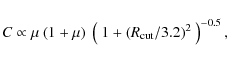
where
We note that we took into account for both Earth emission components the distortion of the surface brightness related to the fact that only a portion of the Earth's hemisphere can be seen when the spacecraft is relatively close to the planet.
![\begin{figure}
\par\includegraphics[bb=16 150 430 700,clip,width=9cm]{13072f2.eps}
\end{figure}](/articles/aa/full_html/2010/04/aa13072-09/img37.png)
|
Figure 2:
Surfaces representing the five IBIS/ISGRI vignetting effects that
affect the incoming radiation until it reaches the detector plane. The
effects are those corresponding to channel 12 ( |
| Open with DEXTER | |
3.3 Instrumental characteristics
As we wanted to fit real detector lightcurves with model lightcurves we needed to take into account the instrumental characteristics of the telescope in the modeling. This does not include detector responses, but all effects attenuating the incoming photon field on its path from outside the telescope until reaching the detector plane. We identified five effects that affected the detector illumination depending on the direction of the incoming radiation and sometimes on its energy. The most obvious effect is the attenuation due to the coded-mask elements which block out about half of the incoming radiation. The second effect is the non-uniform exposure map which is caused by a partial illumination of the detector for a source outside of the fully coded FoV. Another vignetting effect is induced by the Nomex honeycomb structure that supports the coded mask. The two last effects are due to the IBIS/ISGRI spider beams separating the eight detector modules and to the lead shielding of the IBIS telescope tube. The aluminum spider results in opacity at the lowest energies, and the lead shielding of the tube becomes transparent at the highest energies.
The five effects mentioned above are included in the standard IBIS/ISGRI software for image reconstruction and spectral extraction, but as we worked directly with the detector lightcurves, we needed to account for these effects independently. Their modeling as used in this work is described below and is illustrated in Fig. 2, while the overall vignetting effect is shown in Fig. 1.
The coded-mask transparency is ideally of 0.5 since there are as many elements open as closed. This is, however, only true at the center of the FoV. For off-axis sources there is an additional attenuation due to the thickness of 16 mm of the mask elements, which project a wider shadow on the detector for increasing off-axis angles. As the elements are made of tungsten - a strongly absorbing material - it is fair to assume the elements to be completely opaque in the energy range considered here. As we were only interested in the net effect over the full detector plane and in a simple analytical description we approximated the mask pattern as a giant chessboard of 46 equally-sized square elements on a side of 1064 mm. We then properly computed the additional shadow from radiation that crossed the border of the mask elements and did not fall onto the shadow of other elements.
The exposure map of IBIS/ISGRI is basically very simple with a value of 1 in the fully coded FoV and a linear decrease to zero in the partially coded FoV, except in the corners of the image where the decrease is quadratic. When we modeled this, we properly took into account the disposition of the eight modules of the IBIS/ISGRI detector and the two-pixel wide space between them.
The Nomex structure supporting the coded mask of IBIS is absorbing part of the
incoming photons. This is corrected for in the OSA software by off-axis
efficiency maps depending on energy. In 2006, at the time of the EOs,
these maps were still an approximation with only a dependence on the off-axis
angle. We used the new maps introduced in the OSA 6.0 release that do include an
additional azimuthal dependence due to the alignment of the walls of the
hexagonal tubes that the honeycomb structure is made of and also a correction
for the tubes pointing ![]()
![]() away from the center of the FoV; a
misalignment likely due to on-ground manipulations of the spacecraft. We note
that the attenuation by the cosine of the off-axis angle is included in these
maps.
away from the center of the FoV; a
misalignment likely due to on-ground manipulations of the spacecraft. We note
that the attenuation by the cosine of the off-axis angle is included in these
maps.
The eight IBIS/ISGRI detector modules are separated by an aluminum structure
called the ISGRI spider. It is made of one beam along the Z axis and three
perpendicular beams. According to the IBIS experiment interface document part B
(EID-B) the beams have a trapezoidal section with a height of 48 mm a base of 9.5 mm and a wall angle of
![]() resulting in an upper width of 2.8 mm.
The wall angle ensures that the spider is not casting a shadow in the
fully coded FoV. However, in the partially coded FoV, the spider can mask up to
two rows of ISGRI pixels. We modeled this effect in detail for each energy bin
based on the corresponding attenuation length of Al. We found that for some
specific off-axis directions, the ISGRI spider can result in an attenuation of
the radiation on the detector plane of up to
resulting in an upper width of 2.8 mm.
The wall angle ensures that the spider is not casting a shadow in the
fully coded FoV. However, in the partially coded FoV, the spider can mask up to
two rows of ISGRI pixels. We modeled this effect in detail for each energy bin
based on the corresponding attenuation length of Al. We found that for some
specific off-axis directions, the ISGRI spider can result in an attenuation of
the radiation on the detector plane of up to ![]() 5% in the lower energy
bins.
5% in the lower energy
bins.
The last instrumental effect we considered is the IBIS telescope tube
transparency. At higher energies, the tube becomes transparent to radiation from
outside the fully coded FoV, giving an additional contribution to the detector
lightcurves. The tube is made of two vertical walls perpendicular to the Y axis and of two walls inclined with an angle of
![]() transverse to the Z axis. The walls are shielded with glued lead foils. The thickness of the Pb
sheets for each wall is reported in Table 3.2.8.1 of the EID-B (issue 7.0). We
used the values for the four upper sheets of the wall that are relevant for the
calculation of the tube transparency for an off-axis angle up to about 45
transverse to the Z axis. The walls are shielded with glued lead foils. The thickness of the Pb
sheets for each wall is reported in Table 3.2.8.1 of the EID-B (issue 7.0). We
used the values for the four upper sheets of the wall that are relevant for the
calculation of the tube transparency for an off-axis angle up to about 45![]() .
The calculation was done carefully, avoiding radiation further blocked by other
parts of the ISGRI collimating system: the 1 mm thick W shield of the ISGRI
hopper and the 1.2 mm thick W-strips of the side shielding of the mask. The
tube transparency is neglectable at the lower energies, but reaches
.
The calculation was done carefully, avoiding radiation further blocked by other
parts of the ISGRI collimating system: the 1 mm thick W shield of the ISGRI
hopper and the 1.2 mm thick W-strips of the side shielding of the mask. The
tube transparency is neglectable at the lower energies, but reaches ![]() 1%
in channel 12 (see Fig. 2) near the Pb attenuation length edge at
about 75-80 keV and
1%
in channel 12 (see Fig. 2) near the Pb attenuation length edge at
about 75-80 keV and ![]() 6% in the last energy bin. Although this might
seem unrelevant, the cumulated effect on the detector plane from a wide region
outside the FoV is actually far from negligible at these energies.
6% in the last energy bin. Although this might
seem unrelevant, the cumulated effect on the detector plane from a wide region
outside the FoV is actually far from negligible at these energies.
![\begin{figure}
\par\includegraphics[width=9cm]{13072f3.eps}
\end{figure}](/articles/aa/full_html/2010/04/aa13072-09/img41.png)
|
Figure 3:
Model lightcurves of each component for channel 3 ( |
| Open with DEXTER | |
3.4 Construction of model lightcurves
The next step was to construct model lightcurves describing the modulation of the radiation of each component described in Sect. 3.2 as induced by the passage of the Earth through the IBIS/ISGRI FoV. A complete set of model lightcurves is shown in Fig. 3.
3.4.1 Extended components
For the diffuse components - the CXB, the GRXE and the two different Earth
emission components - we constructed the model lightcurves by generating a
series of images of the sky at different times based on the attitude of the
spacecraft and the position of the Earth in the FoV (see Sect. 3.1).
For each individual component, we considered only its own contribution and the
instrumental vignetting effects (see Sect. 3.3) attenuating the
count rates on the detector plane. The sum of the pixels in the images generated
for different times during the Earth occultation defines the model lightcurve
for a given component. Because the instrumental attenuation is energy dependent,
we constructed these model lightcurves for each energy bin and for each of the
four EOs because of the slightly different pointing directions with respect to
the Galactic ridge and Earth positions. As high-energy radiation from outside
the field of view also contributes to the detector counts (see
Sect. 3.3), the simulated images were defined on a wide area
extending 30![]() outside of the actual FoV of IBIS/ISGRI (
outside of the actual FoV of IBIS/ISGRI (
![]() and
and
![]() ).
).
The normalization of the diffuse components in the input images - without
vignetting effects - was set to 10 count s-1 sr-1. For the Earth
emission components, this is the average intensity over the Earth disk, while it
is the average in the area defined by
![]() and
and
![]() for
the GRXE. After attenuation by the instrumental effects described in
Sect. 3.3 the actual detector count rate was typically reduced by an
order of magnitude (see Fig. 3).
for
the GRXE. After attenuation by the instrumental effects described in
Sect. 3.3 the actual detector count rate was typically reduced by an
order of magnitude (see Fig. 3).
3.4.2 Point sources
In addition to the lightcurves constructed for the extended components we also
generated one lightcurve in each energy bin for the point sources in the FoV.
The time modulation is step-like in this case due to the abrupt disappearance of
a source when it gets occultated by the Earth. The count rate used for each
source detected with a significance of more than 2![]() was derived
from a bremsstrahlung fit to its observed IBIS/ISGRI spectrum (see
Sect. 2) divided by the fraction of time during which the source was not
occulted. These counts were then assigned to the corresponding source position
in the simulated sky images, and detector counts were obtained by summing-up the
image pixels after application of the instrumental vignetting effects. We did
this at different times during the passage of the Earth through the FoV to get
model detector lightcurves. As the set of model lightcurves for point sources at
different energies was based on the actual data collected during each EO, they
were considered as a fix contribution to the detector lightcurves.
was derived
from a bremsstrahlung fit to its observed IBIS/ISGRI spectrum (see
Sect. 2) divided by the fraction of time during which the source was not
occulted. These counts were then assigned to the corresponding source position
in the simulated sky images, and detector counts were obtained by summing-up the
image pixels after application of the instrumental vignetting effects. We did
this at different times during the passage of the Earth through the FoV to get
model detector lightcurves. As the set of model lightcurves for point sources at
different energies was based on the actual data collected during each EO, they
were considered as a fix contribution to the detector lightcurves.
3.4.3 Instrumental background
The last but the dominant contributor to the observed detector lightcurves is
the instrumental background. The time variability of this component depends on
the cosmic particle environment and the induced radioactive decay of the
spacecraft's material. The particle environment is well monitored by the
anti-coincidence shield (ACS) of the spectrometer SPI, the other gamma-ray
instrument of INTEGRAL (Vedrenne et al. 2003). We found good evidence that
the IBIS/ISGRI detector lightcurves are indeed following the variations
recorded by the SPI ACS. To estimate the actual relationship between the count
rates in the ACS and in the IBIS/ISGRI detector in each of the considered
spectral bins, we used the extragalactic observations of revolution 342 (Her X-1
and XMM LSS). These observations, away from bright hard X-ray sources, were
taken about six months before the EOs and have the particularity of including a
solar flare at the start of the revolution, resulting in important correlated
variations in the SPI ACS and the ISGRI detector counts during the 12-h decay
of the flare between INTEGRAL Julian dates (IJD = JD
![]() )
of 2040.0 and 2040.5. This relationship is characterized by the slope
)
of 2040.0 and 2040.5. This relationship is characterized by the slope ![]() of a linear fit of the ISGRI counts versus the SPI/ACS counts. This slope is
likely to change from one observation to the other because the orientation of
the spacecraft with respect to the solar radiation and particle flux will change
the effective areas of both the SPI/ACS and the IBIS/ISGRI detectors in a
complex manner. However, the energy dependence of the slope
of a linear fit of the ISGRI counts versus the SPI/ACS counts. This slope is
likely to change from one observation to the other because the orientation of
the spacecraft with respect to the solar radiation and particle flux will change
the effective areas of both the SPI/ACS and the IBIS/ISGRI detectors in a
complex manner. However, the energy dependence of the slope ![]() for
different ISGRI energy bins is expected to be rather stable. We used this
energy dependence of
for
different ISGRI energy bins is expected to be rather stable. We used this
energy dependence of ![]() as an indication of the amount of SPI/ACS
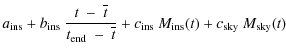
modulation expected in the ISGRI detector lightcurves of the EOs. The model
lightcurve for the variations of the instrumental background was thus
constructed based on those of the SPI/ACS as:
as an indication of the amount of SPI/ACS
modulation expected in the ISGRI detector lightcurves of the EOs. The model
lightcurve for the variations of the instrumental background was thus
constructed based on those of the SPI/ACS as:
where
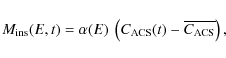
3.5 Spectral fitting
We described above the construction of the model lightcurves Mi(t) shown in
Fig. 3 for each component i,
which are the SPI/ACS-related
variations of the instrumental background (ins), the sky background
(sky), the
GRXE (gal), the Earth's albedo (alb), the atmospheric CR-induced
emission (atm), and the point sources (src) in the FoV. The next step
is to adjust these
model lightcurves to the observed detector lightcurve D(t) in a given energy
band with a least-square fit. This is done by the following linear relation:
where
By fitting the observed lightcurves D(E,t) in different energy bands E, one
derives count rate spectra ci(E) for the five components i. When we did
this independently for each of the 16 energy bins, we obtained quite noisy
spectra with a divergence towards non-plausible values in some channels. This is
due to significant degeneracy between the various components that we discuss in
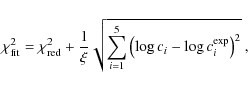
Sect. 5.4. A way to overcome this problem was to include a link in the
fitting between the values obtained in one energy bin and in some others. We did
this by adding an additional constraint to the ![]() minimization of the fit
so that the fitted parameter value ci would not be too far from an expected
value
minimization of the fit
so that the fitted parameter value ci would not be too far from an expected
value
![]() according to:
according to:
where
The choice of the expected values
![]() in this constraint fit can of
course have strong implications on the results. We therefore took great care to
define them without including wrong assumptions and systematic effects. For the
parameter
in this constraint fit can of
course have strong implications on the results. We therefore took great care to
define them without including wrong assumptions and systematic effects. For the
parameter
![]() ,
the expected value was set to be the mean value
obtained over the 16 energy bins. This was motivated by our discussion in
Sect. 3.4.3, where we concluded that this factor can differ from unity, but is
expected to be rather constant from one energy bin to the other. For the four
other ci parameters, we defined the expected value based on the assumption
that the final, unfolded spectrum of each component is supposed to be smooth.
For each component spectrum, ci(E), the expected count rate in a given
channel,
,
the expected value was set to be the mean value
obtained over the 16 energy bins. This was motivated by our discussion in
Sect. 3.4.3, where we concluded that this factor can differ from unity, but is
expected to be rather constant from one energy bin to the other. For the four
other ci parameters, we defined the expected value based on the assumption
that the final, unfolded spectrum of each component is supposed to be smooth.
For each component spectrum, ci(E), the expected count rate in a given
channel,
![]() ,
was set to be the linear interpolation between the
values in the two adjacent energy bins corrected for the effects of different
energy widths of the channels and of the detector response
,
was set to be the linear interpolation between the
values in the two adjacent energy bins corrected for the effects of different
energy widths of the channels and of the detector response![]() . For the first and last energy bins, the spectral
smoothness was similarly constrained, by setting the expected value to the
linear extrapolation of the two closest channels. We note that we did not
constrain the spectrum of the instrumental background level
. For the first and last energy bins, the spectral
smoothness was similarly constrained, by setting the expected value to the
linear extrapolation of the two closest channels. We note that we did not
constrain the spectrum of the instrumental background level
![]() and
its increasing or decreasing trend with time,
and
its increasing or decreasing trend with time,
![]() ,
because both can
change rapidly from one energy bin to the other due to the presence of narrow
emission lines (see Sect. 2). For the five other parameters, the
introduced interdependence of the values obtained in adjacent energy bins
typically reduces the number of free parameters of the fit by a factor of 2.
This was taken into account when calculating the d.o.f. of the fit.
,
because both can
change rapidly from one energy bin to the other due to the presence of narrow
emission lines (see Sect. 2). For the five other parameters, the
introduced interdependence of the values obtained in adjacent energy bins
typically reduces the number of free parameters of the fit by a factor of 2.
This was taken into account when calculating the d.o.f. of the fit.
The actual fitting began with a set of input spectra and minimized the modified
![]() of Eq. (4), one channel after the other. We then reran this
process up to four times until the overall
of Eq. (4), one channel after the other. We then reran this
process up to four times until the overall ![]() - computed on the
lightcurves in all energy bins - did not significantly improve anymore. This
iterative spectral fitting was done independently for each of the four
Earth-observation datasets, and we combined the results to get the final
spectra.
- computed on the
lightcurves in all energy bins - did not significantly improve anymore. This
iterative spectral fitting was done independently for each of the four
Earth-observation datasets, and we combined the results to get the final
spectra.
An issue in the fitting process is the choice of the parameter ![]() that defines the strength of the additional constraint on the fit in
Eq. (4). If
that defines the strength of the additional constraint on the fit in
Eq. (4). If ![]() is low the spectral smoothness constraint becomes
important and it then does not leave enough freedom to fit the actual data,
whereas if
is low the spectral smoothness constraint becomes
important and it then does not leave enough freedom to fit the actual data,
whereas if ![]() is too high, the fit might diverge in some energy bins towards
unrealistic values. We tested different values and chose
is too high, the fit might diverge in some energy bins towards
unrealistic values. We tested different values and chose ![]() ,
which leaves a lot of freedom to the fit, while limiting strong divergence to
only a few energy bins in one of the four EOs, namely EO 3 in the 70-100 keV
range (see Fig. 4).
,
which leaves a lot of freedom to the fit, while limiting strong divergence to
only a few energy bins in one of the four EOs, namely EO 3 in the 70-100 keV
range (see Fig. 4).
Another important issue is the choice of the input parameters, since we
experienced that they can have a significant influence on the final results.
This is due to degeneracy between some components that we discuss in
Sect. 5.4. It is therefore safe to start with values corresponding
roughly to the expectations for the CXB and also for one of the two Earth
emission components. We chose the analytical formula of Gruber et al. (1999) as the
basis for the input CXB spectrum. A first guess of the spectral values of
the other components was obtained by doing a fit with the input CXB spectrum
fixed and imposing equal contributions for the two Earth emission components.
We obtained a global Earth emission that is much lower at the highest
energies than derived by Churazov et al. (2007). As the CR-induced emission of the Earth
is the dominant component at these energies, this suggests that its
normalization has to be scaled down by a factor of ![]() 0.4 (see
Fig. 13). The final set of unperturbated input spectra was
obtained by fitting the lightcurves again, but this time with fixed values for
both the CXB and the CR-induced Earth emission. For the latter, the spectrum was
defined by the analytical formula proposed by Sazonov et al. (2007, Eq. (1)) with a
normalization C of 13.2 keV cm-2 s-1 sr-1, i.e. 0.4 times that derived by
Churazov et al. (2007).
0.4 (see
Fig. 13). The final set of unperturbated input spectra was
obtained by fitting the lightcurves again, but this time with fixed values for
both the CXB and the CR-induced Earth emission. For the latter, the spectrum was
defined by the analytical formula proposed by Sazonov et al. (2007, Eq. (1)) with a
normalization C of 13.2 keV cm-2 s-1 sr-1, i.e. 0.4 times that derived by
Churazov et al. (2007).
![\begin{figure}
\par\includegraphics[width=9cm]{13072f6.eps}
\end{figure}](/articles/aa/full_html/2010/04/aa13072-09/img66.png)
|
Figure 4: IBIS/ISGRI count rate spectra of each model component derived from the detector lightcurves of the INTEGRAL EOs. The values are vignetting-corrected count rates per channel in units of 10 count s-1 sr-1, except for the instrumental background (black diamonds) for which they are actual detector count rates in count s-1. For the CXB (red circles), the GRXE (blue squares) and the total Earth emission (green triangles), the dotted lines of the same color show the average spectra obtained for the four independent EOs. The relative contributions to the Earth emission from the CXB reflection (cyan triangles, long-dashed) and the CR scattering in the atmosphere (magenta triangles, short-dashed) are also shown. |
| Open with DEXTER | |
![\begin{figure}
\par\mbox{\includegraphics[width=6cm]{13072f5a.eps}\includegraphi...
...5b.eps}\includegraphics[width=6cm]{13072f5c.eps} }
\vspace*{-1.5mm}
\end{figure}](/articles/aa/full_html/2010/04/aa13072-09/img67.png)
|
Figure 5:
Examples of detector lightcurve fits ( upper panels) and associated residuals ( lower panels) for the first EO at three representative energies: |
| Open with DEXTER | |
To smear-out the dependence of the final results on these input spectra
and to estimate the uncertainties, we made a series of fits with different
input parameter values. We did this by perturbating each channel value of the
initial spectra by a random deviation following a Gaussian distribution with a
![]() of 30%. This was done independently for all five component spectra,
namely the CXB, the GRXE, the two Earth emission components and the
average level of the instrumental background. We performed the whole
fitting
process described above starting from 30 different sets of perturbated
input
spectra. For the four EOs, this resulted in 120 spectral fits.
Instead of taking the average on the obtained values, we took the
median in each energy bin
as a robust estimator of the mean. This has the advantage to be
independent of
the use of the actual results or of their logarithm and is not
influenced by
outstanding values. We estimated the 1-
of 30%. This was done independently for all five component spectra,
namely the CXB, the GRXE, the two Earth emission components and the
average level of the instrumental background. We performed the whole
fitting
process described above starting from 30 different sets of perturbated
input
spectra. For the four EOs, this resulted in 120 spectral fits.
Instead of taking the average on the obtained values, we took the
median in each energy bin
as a robust estimator of the mean. This has the advantage to be
independent of
the use of the actual results or of their logarithm and is not
influenced by
outstanding values. We estimated the 1-![]() (68% CL) statistical
uncertainties on the median taking the two results at
(68% CL) statistical
uncertainties on the median taking the two results at
![]() in rank order away from the median, where the
factor of four stands for the four EOs being independent measurements.
in rank order away from the median, where the
factor of four stands for the four EOs being independent measurements.
4 Results
Table 3: Spectral fit parameters for the CXB, the GRXE and the Earth emission.
The count rate spectra and uncertainties obtained with the iterative spectral
fitting process described in Sect. 3.5 are shown in Fig. 4.
We note that the large scatter from one EO to the other is clearly
dominating the uncertainties, which suggests that performing additional EOs in
the future will allow us to significantly improve the statistics of the
results. We obtained overall average reduced ![]() values of
values of
![]() = 1.20, 1.11, 1.15 and 1.13 for EO 1 to EO 4,
respectively. These values only slightly above unity show that we get a fair
description of all the lightcurves, without overinterpreting the data by using
too many free parameters. As an example we show the match between the model
corresponding to the final results for EO 1 and the observed lightcurves in
three representative channels in Fig. 5.
= 1.20, 1.11, 1.15 and 1.13 for EO 1 to EO 4,
respectively. These values only slightly above unity show that we get a fair
description of all the lightcurves, without overinterpreting the data by using
too many free parameters. As an example we show the match between the model
corresponding to the final results for EO 1 and the observed lightcurves in
three representative channels in Fig. 5.
The count rate spectra ci(E) shown in Fig. 4 correspond to the
values before entering the telescope, i.e. they are corrected for the
instrumental vignetting effects described in Sect. 3.3. We could
thus directly use them for spectral fitting with XSpec to get unfolded spectra
in physical units. We did the spectral fitting with the standard IBIS/ISGRI ARF
and RMF detector response files distributed with OSA 7.0. We did not consider
Galactic hydrogen absorption in the fit because even along the galactic plane
the hydrogen column density is small enough -
![]() cm-2 at Galactic coordinates of (l,b) = (330
cm-2 at Galactic coordinates of (l,b) = (330![]() ,
0
,
0![]() )
- to have only a negligible effect. The spectral fit parameters are given in Table 3 and the resulting unfolded spectra are shown in
Fig. 6 with the numerical values given in Table 2.
)
- to have only a negligible effect. The spectral fit parameters are given in Table 3 and the resulting unfolded spectra are shown in
Fig. 6 with the numerical values given in Table 2.
![\begin{figure}
\par\includegraphics[width=9cm]{13072f4.eps}
\end{figure}](/articles/aa/full_html/2010/04/aa13072-09/img74.png)
|
Figure 6: Unfolded IBIS/ISGRI spectra of the sky background (red circles), the earth emission (green triangles) and the GRXE (blue squares) with their best fit (dashed lines) and the more physical (dotted lines) spectral models (see Tables 2 and 3). The contribution of the sum of the considered point sources averaged over the four EOs is also shown (orange stars). |
| Open with DEXTER | |
The CXB spectrum is best fitted by a broken powerlaw model with a break
energy at
![]() keV and a high-energy photon index of
keV and a high-energy photon index of
![]() ,
giving a reduced chi-squared of
,
giving a reduced chi-squared of
![]() for 12 d.o.f. A more physical model for the CXB
emission - considered as the superimposition of the emission of unresolved
Seyfert galaxies - is to take a cut-off powerlaw model. The degeneracy between
spectral slope and cut-off energy was solved by fixing the photon index to the
value of
for 12 d.o.f. A more physical model for the CXB
emission - considered as the superimposition of the emission of unresolved
Seyfert galaxies - is to take a cut-off powerlaw model. The degeneracy between
spectral slope and cut-off energy was solved by fixing the photon index to the
value of
![]() derived by Beckmann et al. (2009) on average for all Seyfert
galaxies detected by INTEGRAL. We then obtained a good description of the CXB spectrum
derived by Beckmann et al. (2009) on average for all Seyfert
galaxies detected by INTEGRAL. We then obtained a good description of the CXB spectrum
![]() with a cut-off energy of
with a cut-off energy of
![]() keV, at slightly higher energy than E = 86 keV derived for Seyfert 1 galaxies (Beckmann et al. 2009).
keV, at slightly higher energy than E = 86 keV derived for Seyfert 1 galaxies (Beckmann et al. 2009).
We found that the GRXE spectrum was best fitted by a cut-off powerlaw plus a
second powerlaw to account for the hard tail at energies above ![]() 80 keV.
As the indices of the powerlaws are poorly constrained, we fixed their
values to
80 keV.
As the indices of the powerlaws are poorly constrained, we fixed their
values to
![]() for the cut-off powerlaw and to
for the cut-off powerlaw and to
![]() for the hard tail, as derived by Bouchet et al. (2008). This gives a very good
description of the data with a
for the hard tail, as derived by Bouchet et al. (2008). This gives a very good
description of the data with a
![]() for 13 d.o.f.
According to Revnivtsev et al. (2006), the main population contributing to the low-energy
part of the GRXE are intermediate polar cataclysmic variables. The accretion
column onto the magnetic poles of such types of accreting white dwarfs is
emitting optically thin thermal emission. The best fit for this more physical
bremsstrahlung model is almost undistinguishable from the cut-off powerlaw (see
Fig. 6) and gives a typical average temperature of
for 13 d.o.f.
According to Revnivtsev et al. (2006), the main population contributing to the low-energy
part of the GRXE are intermediate polar cataclysmic variables. The accretion
column onto the magnetic poles of such types of accreting white dwarfs is
emitting optically thin thermal emission. The best fit for this more physical
bremsstrahlung model is almost undistinguishable from the cut-off powerlaw (see
Fig. 6) and gives a typical average temperature of
![]() .
.
The spectrum of the total Earth emission is best fitted by a broken
powerlaw with a break at
![]() keV and a high-energy photon index
of
keV and a high-energy photon index
of
![]() .
This break energy is slightly higher than derived by the recent analysis of the Swift/BAT data by Ajello et al. (2008), while the obtained spectral slope is in remarkable agreement with their result of
.
This break energy is slightly higher than derived by the recent analysis of the Swift/BAT data by Ajello et al. (2008), while the obtained spectral slope is in remarkable agreement with their result of
![]() (90% CL errors). We found a different
normalization of the Earth emission spectrum however, which we discuss in
Sect. 5.3, where we also discuss the separate spectra obtained for the
albedo and the CR-induced emission.
(90% CL errors). We found a different
normalization of the Earth emission spectrum however, which we discuss in
Sect. 5.3, where we also discuss the separate spectra obtained for the
albedo and the CR-induced emission.
The spectrum of the sum of all point sources detected at more than
2![]() on average among the 4 EOs is added in Fig. 6
for
comparison. The impression that point sources contribute much less than
the GRXE is misleading. This is related to the arbitrary area we chose
for the
normalization of the GRXE. If we had normalized it to the area actually
covered
by the partially coded FoV of IBIS, we would have had a GRXE spectrum
scaled
down by a factor of
on average among the 4 EOs is added in Fig. 6
for
comparison. The impression that point sources contribute much less than
the GRXE is misleading. This is related to the arbitrary area we chose
for the
normalization of the GRXE. If we had normalized it to the area actually
covered
by the partially coded FoV of IBIS, we would have had a GRXE spectrum
scaled
down by a factor of ![]() 4, depending a bit on the EO. This would then lead to
a higher contribution of the point sources compared to the GRXE in qualitative
agreement with the SPI results by Bouchet et al. (2008).
4, depending a bit on the EO. This would then lead to
a higher contribution of the point sources compared to the GRXE in qualitative
agreement with the SPI results by Bouchet et al. (2008).
5 Discussion
The spectra in the ![]() 20-200 keV range presented above will now be
compared to previously published INTEGRAL
results and to spectra obtained by other satellites. In the subsections
below, we discuss this separately for the CXB spectrum, the GRXE and
the Earth emission.
20-200 keV range presented above will now be
compared to previously published INTEGRAL
results and to spectra obtained by other satellites. In the subsections
below, we discuss this separately for the CXB spectrum, the GRXE and
the Earth emission.
5.1 Sky background spectrum
It is interesting to compare the CXB spectrum obtained by the thorough analysis of the IBIS/ISGRI detector lightcurves presented here with the INTEGRAL results previously published by Churazov et al. (2007). The comparison is shown in Fig. 7. Our approach could significantly increase the useful energy range of the IBIS/ISGRI data towards higher energies. The new results fall slightly below the previous IBIS/ISGRI spectrum, while we get a good agreement with the SPI results of Churazov et al. (2007), except possibly for the first energy bin.
![\begin{figure}
\par\includegraphics[width=8.5cm,clip]{13072f7.eps}
\end{figure}](/articles/aa/full_html/2010/04/aa13072-09/img88.png)
|
Figure 7: Comparison of the IBIS/ISGRI CXB spectrum obtained here (red circles) with the previous INTEGRAL results of IBIS/ISGRI (black diamonds), JEM-X (blue squares) and SPI (green triangles) published by Churazov et al. (2007). |
| Open with DEXTER | |
![\begin{figure}
\par\includegraphics[bb=16 144 600 510,clip,width=9cm]{13072f8.eps}
\end{figure}](/articles/aa/full_html/2010/04/aa13072-09/img89.png)
|
Figure 8: Comparison of the CXB spectrum obtained by INTEGRAL - JEM-X measurements (blue squares) from Churazov et al. (2007) and our IBIS/ISGRI results (red circles) - with the HEAO-1 spectra and analytical model by Gruber et al. (1999) (error bars and dashed line). The data of the A-4 instrument of HEAO-1 are shown in green with original normalization, while we show in orange the spectrum of the A-2 instrument and of the model, both increased by 10% in intensity. |
| Open with DEXTER | |
![\begin{figure}
\par\includegraphics[bb=16 144 600 510,clip,width=9cm]{13072f9.eps}
\end{figure}](/articles/aa/full_html/2010/04/aa13072-09/img90.png)
|
Figure 9: Comparison of the INTEGRAL IBIS/ISGRI (red circles, this work) and JEM-X (magenta diamonds, Churazov et al. 2007) spectra with the other recent CXB measurements by Swift and BeppoSAX. The Swift/XRT error box (orange shaded area) and the Swift/BAT results (green triangles) are from Moretti et al. (2009) and Ajello et al. (2008), respectively. The best-fit model of Moretti et al. (2009) for the combined Swift dataset is shown with a black line and grey uncertainty area. The original BeppoSAX/PDS measurements of Frontera et al. (2007) were scaled by +13% in intensity (blue squares) to correct for the difference in Crab normalization with respect to INTEGRAL. The analytical model we propose in Eq. (5) is shown as a purple dashed line. |
| Open with DEXTER | |
As shown in Fig. 8, the slightly lower emission we obtain now with IBIS/ISGRI is consistent with the HEAO-1 measurements and its analytical approximation by Gruber et al. (1999). The flux scaling of the HEAO-1 spectrum by +10% as suggested by Churazov et al. (2007) is actually not required anymore in the IBIS/ISGRI energy range. The discrepancy appears only below 20 keV for the INTEGRAL/JEM-X data that indicate a higher CXB intensity than the HEAO-1 measurements. It seems therefore that a simple scaling in intensity of the historic HEAO-1 spectrum is not able to consistently adjust the combined CXB measurements of INTEGRAL, both below and above the turnover.
However, as illustrated in Fig. 8, there is some freedom
within the uncertainties to scale up by ![]() 10% the intensity of the
spectrum of the A-2 instrument of HEAO-1
without changing that of the A-4 experiment. This would better
match the JEM-X measurements and other results by recent X-ray
instruments, which all suggest a higher intensity below 20 keV
than obtained by HEAO-1/A-2 (e.g. Gilli et al. 2007,
Fig. 15). The net effect
would be a broadening of the CXB hump and a slight shift of its maximum
towards
lower energies. The expected qualitative consequence for an AGN
population
synthesis of the CXB would be a reduction of the contribution of the
most highly obscured AGN, in particular the Compton-thick ones (e.g. Treister et al. 2009). Alternatively, it could also indicate a slightly stronger contribution from a
population of distant (redshifted) luminous AGN compared to the local population (e.g. Treister & Urry 2005).
10% the intensity of the
spectrum of the A-2 instrument of HEAO-1
without changing that of the A-4 experiment. This would better
match the JEM-X measurements and other results by recent X-ray
instruments, which all suggest a higher intensity below 20 keV
than obtained by HEAO-1/A-2 (e.g. Gilli et al. 2007,
Fig. 15). The net effect
would be a broadening of the CXB hump and a slight shift of its maximum
towards
lower energies. The expected qualitative consequence for an AGN
population
synthesis of the CXB would be a reduction of the contribution of the
most highly obscured AGN, in particular the Compton-thick ones (e.g. Treister et al. 2009). Alternatively, it could also indicate a slightly stronger contribution from a
population of distant (redshifted) luminous AGN compared to the local population (e.g. Treister & Urry 2005).
Another consistency check of our results is to compare them to the recent
Swift and BeppoSAX measurements. This is illustrated in
Fig. 9 where the Swift/XRT and the Swift/BAT spectra
are from Moretti et al. (2009) and Ajello et al. (2008), respectively. Our data are consistent
with the Swift/BAT results and the combined XRT-BAT spectral model
proposed by Moretti et al. (2009), although they tend to be at a significantly lower
intensity. Our data agree very well with the BeppoSAX/PDS data
(Frontera et al. 2007, Fig. 6 Bottom) provided that they are scaled by a factor of
1.13 in intensity to account for the difference in the Crab normalization in the 20-50 keV band between BeppoSAX/PDS
(Frontera et al. 2007,
![]() erg cm-2 s-1) and
INTEGRAL (Churazov et al. 2007,
erg cm-2 s-1) and
INTEGRAL (Churazov et al. 2007,
![]() erg cm-2 s-1).
We note that the latter estimation for INTEGRAL is fully consistent with
the value obtained with OSA 7.0. The measured fluxes are
erg cm-2 s-1).
We note that the latter estimation for INTEGRAL is fully consistent with
the value obtained with OSA 7.0. The measured fluxes are
![]() erg cm-2 s-1 and
erg cm-2 s-1 and
![]() erg cm-2 s-1 for the Crab observations of revolutions 365
and 422, respectively.
The obtained spectrum seems to be also very consistent in the peak region
with the recent CXB synthesis model by Treister et al. (2009). It thus gives additional
evidence for a small Compton-thick AGN fraction in the CXB spectrum, close to
9% instead about 30-40% postulated before (e.g. Treister & Urry 2005). Our data
cannot constrain a possible hardening of the CXB spectrum above 100 keV, but
are consistent with an additional contribution of flat-spectrum radio quasars,
which have been found to dominate the CXB in the MeV range (Ajello et al. 2009).
erg cm-2 s-1 for the Crab observations of revolutions 365
and 422, respectively.
The obtained spectrum seems to be also very consistent in the peak region
with the recent CXB synthesis model by Treister et al. (2009). It thus gives additional
evidence for a small Compton-thick AGN fraction in the CXB spectrum, close to
9% instead about 30-40% postulated before (e.g. Treister & Urry 2005). Our data
cannot constrain a possible hardening of the CXB spectrum above 100 keV, but
are consistent with an additional contribution of flat-spectrum radio quasars,
which have been found to dominate the CXB in the MeV range (Ajello et al. 2009).
Based on the considerations above, we can tentatively suggest a slight
adaptation of the analytical description of the CXB proposed by
Moretti et al. (2009, Eq. (4)), as:
where the only difference - but a correction of a typo in the units - is a change of the break energy from 29 keV to 28 keV. The corresponding spectral shape is at the lower limit of the uncertainty area of the Swift model as shown in Fig. 9.
5.2 Galactic ridge emission
![\begin{figure}
\par\includegraphics[bb=16 144 600 510,clip,width=9cm]{13072f10.eps}
\end{figure}](/articles/aa/full_html/2010/04/aa13072-09/img96.png)
|
Figure 10:
Comparison of the obtained GRXE spectrum (blue squares) with recent
other determinations, all renormalized to the central radian of the
Milky Way defined by
|
| Open with DEXTER | |
It is not easy to compare results on the GRXE from one publication to the other,
because the emission is often defined in different regions of the Galaxy. As the
region covered by our observations is away from the Galactic bulge where most
determinations have been made, we have to rescale them to a more commonly used
area. We choose the central radian of the Milky Way defined in Galactic
longitude l and latitude b by
![]() and
and
![]() as the
reference area for a comparison of the various measurements. As we do have an
analytical model of the GRXE (see Sect. 3.2), it is possible to determine
the scaling factor from any region in the Galaxy to the chosen area. The
resulting renormalized spectra are compared in Fig. 10. Our
measurements had to be scaled by a factor of 0.16 to correspond to the chosen
area. The INTEGRAL/IBIS spectrum from Krivonos et al. (2007, Fig. 14)
corresponding to the IBIS FoV area centered on the Galactic bulge was
multiplied by a calculated factor of 2.77. We used the same factor for the
RXTE/PCA data that have been scaled by Krivonos et al. (2007) to match the IBIS
measurement at 20 keV. For the INTEGRAL/SPI spectrum of
Bouchet et al. (2008, Fig. 9) that correspond already to the area chosen here, we just
had to convert the units.
as the
reference area for a comparison of the various measurements. As we do have an
analytical model of the GRXE (see Sect. 3.2), it is possible to determine
the scaling factor from any region in the Galaxy to the chosen area. The
resulting renormalized spectra are compared in Fig. 10. Our
measurements had to be scaled by a factor of 0.16 to correspond to the chosen
area. The INTEGRAL/IBIS spectrum from Krivonos et al. (2007, Fig. 14)
corresponding to the IBIS FoV area centered on the Galactic bulge was
multiplied by a calculated factor of 2.77. We used the same factor for the
RXTE/PCA data that have been scaled by Krivonos et al. (2007) to match the IBIS
measurement at 20 keV. For the INTEGRAL/SPI spectrum of
Bouchet et al. (2008, Fig. 9) that correspond already to the area chosen here, we just
had to convert the units.
In general, Fig. 10 shows a good agreement between the results of the
various instruments. This is quite remarkable for data that were not arbitrarily
renormalized, but were rescaled based on our very simple double-Lorentzian model
of the GRXE. This suggests that the model provides a fair description of the
overall emission of the inner Galaxy in the hard X-ray range. All three
independent INTEGRAL measurements reveal a minimum at about 80 keV. This
was only suggested by the 2-![]() upper limits of Krivonos et al. (2007), but is
confirmed now by our Earth occultation results and the latest SPI results of
Bouchet et al. (2008). Our IBIS/ISGRI results do, however, suggest that the
minimum is shallower than previously found. The diffuse GRXE below 80 keV is
thought to be due to a population of accreting white dwarfs too faint to be
resolved into discrete sources in the hard X-rays (Revnivtsev et al. 2006; Krivonos et al. 2007). It is only at energies of
upper limits of Krivonos et al. (2007), but is
confirmed now by our Earth occultation results and the latest SPI results of
Bouchet et al. (2008). Our IBIS/ISGRI results do, however, suggest that the
minimum is shallower than previously found. The diffuse GRXE below 80 keV is
thought to be due to a population of accreting white dwarfs too faint to be
resolved into discrete sources in the hard X-rays (Revnivtsev et al. 2006; Krivonos et al. 2007). It is only at energies of ![]() 6-7 keV that the diffuse emission could finally be
resolved using deep Chandra observations (Revnivtsev et al. 2009). The
bremsstrahlung temperature of
6-7 keV that the diffuse emission could finally be
resolved using deep Chandra observations (Revnivtsev et al. 2009). The
bremsstrahlung temperature of
![]() that we derived in
Sect. 4 for the accretion column onto the pole of the white dwarfs
agrees well with the measurements of individual intermediate polar systems
detected by Swift/BAT (Brunschweiger et al. 2009). Based on Table 2 in the latter
publication, we note that this temperature would correspond to a typical white
dwarf mass of
that we derived in
Sect. 4 for the accretion column onto the pole of the white dwarfs
agrees well with the measurements of individual intermediate polar systems
detected by Swift/BAT (Brunschweiger et al. 2009). Based on Table 2 in the latter
publication, we note that this temperature would correspond to a typical white
dwarf mass of
![]() according to the
model of Suleimanov et al. (2005). This estimate is just slightly above the expected
average mass of white dwarfs in the Galaxy
(
according to the
model of Suleimanov et al. (2005). This estimate is just slightly above the expected
average mass of white dwarfs in the Galaxy
(
![]() )
that was found to agree well
with the previous IBIS/ISGRI results on the GRXE (Krivonos et al. 2007, and references
therein).
)
that was found to agree well
with the previous IBIS/ISGRI results on the GRXE (Krivonos et al. 2007, and references
therein).
![\begin{figure}
\par\includegraphics[bb=16 144 600 510,clip,width=9cm]{13072f11.eps}
\end{figure}](/articles/aa/full_html/2010/04/aa13072-09/img101.png)
|
Figure 11:
Comparison of the obtained GRXE spectrum (blue error bars and
long-dashed line) with the higher-energy emission of the Galactic ridge
in the region defined by
|
| Open with DEXTER | |
Above 80 keV the GRXE spectrum is likely dominated by inverse-Compton emission
from the interstellar medium (Porter et al. 2008). We derived an intensity at
the level of the 2-![]() upper limits of Krivonos et al. (2007), in excellent
agreement with the latest SPI observations (Bouchet et al. 2008). The photon
index of the high-energy powerlaw derived by these authors (
upper limits of Krivonos et al. (2007), in excellent
agreement with the latest SPI observations (Bouchet et al. 2008). The photon
index of the high-energy powerlaw derived by these authors (
![]() )
also agrees very well with our results, although it is too poorly constrained by our data alone to be fitted independently.
)
also agrees very well with our results, although it is too poorly constrained by our data alone to be fitted independently.
The overall shape of the high-energy spectrum of the GRXE including the
observations of the Compton gamma-ray observatory (CGRO) up to 10 GeV is
shown in Fig. 11. As our data are scaled from a region at
![]() lying outside the galactic bulge where the bulk of the
positronium annihilation is emitted, they should be almost unaffected by the
positronium continuum. This implies that the
lying outside the galactic bulge where the bulk of the
positronium annihilation is emitted, they should be almost unaffected by the
positronium continuum. This implies that the ![]() 20% higher normalization
of the high-energy powerlaw suggested by our data should be intrinsic. This
would agree well with the discussion of Porter et al. (2008) concerning a possible
higher normalization of up to 40% for this powerlaw.
20% higher normalization
of the high-energy powerlaw suggested by our data should be intrinsic. This
would agree well with the discussion of Porter et al. (2008) concerning a possible
higher normalization of up to 40% for this powerlaw.
5.3 Earth emission
![\begin{figure}
\par\includegraphics[bb=16 144 600 510,clip,width=9cm]{13072f12.eps}
\end{figure}](/articles/aa/full_html/2010/04/aa13072-09/img103.png)
|
Figure 12: Comparison of the obtained Earth emission spectrum (green triangles) with previous determinations by various missions. The thin grey line is the INTEGRAL spectrum of Churazov et al. (2007) as described in Fig. 13. The obtained IBIS/ISGRI spectrum lies well between the OSO-3 (black diamonds) and the Swift/BAT (red circles) measurements of Schwartz & Peterson (1974) and Ajello et al. (2008), respectively. The values of the BeppoSAX/PDS measurements of Frontera et al. (2007) were increased by 13% (blue squares) to be consistent with Fig. 9. |
| Open with DEXTER | |
Before discussing the relative contributions of the two Earth emission components, we first compare, in Fig. 12, the obtained spectrum of the Earth with other determinations. The Earth emission is found to be very consistent with the spectra obtained previously, although there is a big scatter among the various determinations. This is at least partially due to the modulation of the Earth emission by the solar cycle and a dependence of the observed flux on the spacecraft altitude and the geomagnetic latitude (Sazonov et al. 2007). For instance, the difference in normalization between the Swift/BAT spectrum and our determination can be related to INTEGRAL drifting towards an almost polar orbit, while Swift has a more equatorial orbit. The difference by roughly a factor of two depending on the energy is consistent with the difference found by the polar-orbiting satellite 1972-076B between the equatorial and the polar regions (Imhof et al. 1976). We did not include these spectra here for the sake of clarity, but they would be compatible with the other determinations provided that they are corrected for unsubtracted CXB emission as shown by Ajello et al. (2008, Figs. 15 and 16).
A discrepancy we cannot ascribe to a different observation epoch or a different viewpoint is the inconsistency of our results with the spectrum derived from the same INTEGRAL observations by Churazov et al. (2007). We derive a higher Earth emission at low energies and a lower intensity at high energies. The discrepancy at the highest energies could somehow be due to the fact that our results are based on IBIS data and their results on SPI, although both instruments are well cross-calibrated. It is also possible that the difference comes from our more detailed modeling of several instrumental effects described in Sect. 3.3. At the lowest energies, the neglection of point source emission by Churazov et al. (2007) is a likely cause of the discrepancy, since for a given CXB we need more Earth emission to compensate for the occultation of point sources.
![\begin{figure}
\par\includegraphics[bb=16 144 600 510,clip,width=9cm]{13072f13.eps}
\vspace*{6mm}
\end{figure}](/articles/aa/full_html/2010/04/aa13072-09/img104.png)
|
Figure 13: Resulting spectrum of the total Earth emission (green triangles, solid line) with separated contributions from the Earth reflection of the CXB (cyan triangles, short-dashed line) and the CR-induced atmospheric emission (magenta triangles, long-dashed line). The thin grey curves are normalized as derived by Churazov et al. (2007), whereas the thick colored lines are normalized to match our measurements. |
| Open with DEXTER | |
To better characterize the difference between the two determinations of
the Earth spectrum, we show in Fig. 13 the decomposition of the
overall Earth emission in the two distinct components considered in both
studies. Those are the reflection of the CXB by the Earth - the albedo - and
the emission induced by CR interactions in the atmosphere. The spectra of both
components can be described by analytical functions fitted to the results of
Monte-Carlo simulations published by Churazov et al. (2008) for the albedo, and by
Sazonov et al. (2007) for the atmospheric
emission. In order to fit the overall spectrum of the Earth with these
two components, we need to increase the albedo component by ![]() 40% and decrease the atmospheric emission by
40% and decrease the atmospheric emission by ![]() 60% compared
to the normalizations suggested by Churazov et al. (2007). We thus get a normalization of the atmospheric emission (Sazonov et al. 2007, Eq. (1)) of
60% compared
to the normalizations suggested by Churazov et al. (2007). We thus get a normalization of the atmospheric emission (Sazonov et al. 2007, Eq. (1)) of
![]() at the
break energy of E = 44 keV, instead of
at the
break energy of E = 44 keV, instead of
![]() as derived by
Churazov et al. (2007). This difference in normalization is much more important than the
few percent of likely overestimation mentioned by Sazonov et al. (2007) related to the
inclusion of the Compton-scattering from particles that would have intersected
the surface of the Earth. Further speculations on the origin of this discrepancy are beyond the scope of this paper.
as derived by
Churazov et al. (2007). This difference in normalization is much more important than the
few percent of likely overestimation mentioned by Sazonov et al. (2007) related to the
inclusion of the Compton-scattering from particles that would have intersected
the surface of the Earth. Further speculations on the origin of this discrepancy are beyond the scope of this paper.
Concerning the albedo, we note that the increase by a factor 1.4 we
derive here is not on the Earth reflection expected for the HEAO-1
analytic approximation of Gruber et al. (1999), but on this spectrum already scaled by a factor of 1.1 according to the results of Churazov et al. (2007). As the CXB spectrum obtained here agrees well with the original HEAO-1 spectrum, our results suggest a reflection efficiency of the Earth atmosphere ![]() 50%
higher than obtained by the Monte-Carlo simulations of Churazov et al. (2008). According
to these authors, the shape of the input CXB spectrum has only a very limited
effect on the reflected spectrum, especially at energies below
50%
higher than obtained by the Monte-Carlo simulations of Churazov et al. (2008). According
to these authors, the shape of the input CXB spectrum has only a very limited
effect on the reflected spectrum, especially at energies below ![]() 30 keV,
so
there must be another reason for the important difference we observe.
One
possibility is related to the delicate modeling of the composition of
the
atmosphere. Could the presence of clouds have a significant effect by
increasing the amount of hydrogen atoms in the upper atmosphere,
resulting in a more ``Sun-like'' albedo with more reflection at the
lower energies
(see Churazov et al. 2008, Fig. 6)? Another possibility would be the presence of
another Earth emission component emerging at the lowest energies, in particular
the potentially strong X-ray emission of aurorae (e.g. Østgaard et al. 2001). We note that Churazov et al. (2007) found clear evidence for auroral emission in the
INTEGRAL/JEM-X data during EO 2 and EO 3.
30 keV,
so
there must be another reason for the important difference we observe.
One
possibility is related to the delicate modeling of the composition of
the
atmosphere. Could the presence of clouds have a significant effect by
increasing the amount of hydrogen atoms in the upper atmosphere,
resulting in a more ``Sun-like'' albedo with more reflection at the
lower energies
(see Churazov et al. 2008, Fig. 6)? Another possibility would be the presence of
another Earth emission component emerging at the lowest energies, in particular
the potentially strong X-ray emission of aurorae (e.g. Østgaard et al. 2001). We note that Churazov et al. (2007) found clear evidence for auroral emission in the
INTEGRAL/JEM-X data during EO 2 and EO 3.
Finally, it is fair to mention that the almost perfect agreement we show in Fig. 13 between the data and the model for the two distinct Earth emission components is mainly due to the choice of the input spectrum for the atmospheric emission (see Sect. 3.5). The strong degeneracy between the two Earth emission components discussed in Sect. 5.4 does not allow us to get such a good distinction of the two components when starting from an arbitrary set of input parameters. We would just get a tendency for the CR-induced emission to dominate at the higher energies and vice-versa at low energy.
5.4 Degeneracy issues
Degeneracy is the reason why it is so difficult to determine the CXB spectrum with Earth-occultation data. The basic problem is that a spatially uniform Earth emission cannot be distinguished from the CXB occultation when the instrumental background level is unknown. It is because of this that all previous studies using the Earth as occultator had to assume a priori the spectrum of the CXB and to a large extend also that of the Earth emission (see Ajello et al. 2008; Frontera et al. 2007; Churazov et al. 2007). Here, we tried to solve the degeneracy issue by fixing the spatial distribution of the Earth emission components rather than its spectral shape and by introducing a spectral smoothness constraint as explained in Sect. 3.5. However, because of the noise in the data and a possible deviation of the actual instrumental background variations compared to those assumed based on the SPI/ACS lightcurve (see Sect. 3.4.3) it is not possible to completely solve the degeneracy issues.
To overcome this problem, we had also to incorporate some a priori assumptions on the spectral shape of the CXB and of one of the two Earth emission components, chosen to be the atmospheric CR-induced emission because of its strong drop at low energies that cannot be easily determined otherwise. As explained in Sect. 3.5, this is however only used to define the set of input spectra that we then perturbate randomly before fitting the parameters to the data. Despite this, we still keep a dependence on the input parameters in the results. This is very obvious for the two Earth emission components that are strongly degenerated (see Sect. 5.3).
Another important degeneracy is between the instrumental background and the sum
of the sky background plus Earth emission. A higher instrumental background will
imply lower sky background and Earth emission, and vice-versa. Actually, the
data do primarily constrain the difference between the Earth and the CXB
emissions. This difference is basically the height of a bump in the lightcurve
in case the Earth emission dominates or, alternatively, the depth of a trough,
when the sky background occultation dominates (see Fig. 5). To
test the effect of this degeneracy on our results, we fitted the data with the
same procedure as explained in Sect. 3.5, but with an input spectrum for the CXB increased by 10%. This resulted in a CXB spectrum with a similar
shape, but a higher normalization by about the same factor. However, to
compensate this, the Earth albedo is then found to be higher than derived by
Churazov et al. (2007) by a factor of ![]() 2, instead of
2, instead of ![]() 1.4 (see Sect. 5.3).
Although this cannot be completely excluded, the discrepancy on the
normalization of the albedo is judged to be unrealistically high. We
thus favor the more conservative results obtained with the original
normalization of the
CXB for the input parameters.
1.4 (see Sect. 5.3).
Although this cannot be completely excluded, the discrepancy on the
normalization of the albedo is judged to be unrealistically high. We
thus favor the more conservative results obtained with the original
normalization of the
CXB for the input parameters.
The presence of the GRXE in the observed region of the sky can also add some degeneracy, but its location to the side of the FoV was actually rather optimal as its maximal occultation effect occurred earlier in the lightcurves than for the CXB (see Fig. 3). We only noted a slight degeneracy between the GRXE and the sum of the CXB and the polar-enhanced atmospheric emission.
We identified an instrumental effect that affects the results of
both the GRXE and of the Earth emission at energies above ![]() 60 keV. By
ignoring the possibility of an increasing or decreasing trend of the
instrumental background in addition to the SPI/ACS modulation (see Eq. (3)),
we obtained a high-energy drop of the Earth emission together with an
unrealistically steep rise of the GRXE spectrum. This behavior aims at
compensating a decreasing trend of the instrumental counts in the spectral
region of the emission lines of W, Pb and Bi (60-80 keV, see Sect. 2)
and an increasing trend of the counts at even higher energies. This is likely
due to radioactive decay at the exit of the radiation belts and illustrates the
sensitivity of the method on a very accurate description of all instrumental
effects.
60 keV. By
ignoring the possibility of an increasing or decreasing trend of the
instrumental background in addition to the SPI/ACS modulation (see Eq. (3)),
we obtained a high-energy drop of the Earth emission together with an
unrealistically steep rise of the GRXE spectrum. This behavior aims at
compensating a decreasing trend of the instrumental counts in the spectral
region of the emission lines of W, Pb and Bi (60-80 keV, see Sect. 2)
and an increasing trend of the counts at even higher energies. This is likely
due to radioactive decay at the exit of the radiation belts and illustrates the
sensitivity of the method on a very accurate description of all instrumental
effects.
Finally, we note that an underestimation of the contribution of the point sources will tend to increase both the GRXE and the CXB intensity because point sources are distributed all over the FoV with increased density in the galactic plane.
6 Conclusion
We presented the results of an original analysis of the four consecutive Earth-occultation observations by the IBIS/ISGRI instrument aboard the INTEGRAL satellite. Our approach is complementary to the previous study of these data by Churazov et al. (2007), because instead of fixing the spectral shape of the CXB and fitting its normalization, we attempt to derive the complete spectral information from the observed detector lightcurves in different energy bins. This requires a deep understanding of the instrumental effects and a careful modeling of the spatial distribution of the various contributions from the Galaxy, the Earth and point sources. Despite inherent degeneracy issues that forced us to fit the data with an additional spectral smoothness constraint and adequate input parameters, the approach used here results in a coherent set of spectra for the CXB, the GRXE and the Earth emission.
The obtained IBIS/ISGRI results for the CXB are consistent with the historic HEAO-1 spectrum, without any scaling in intensity. The scaling by +10% in intensity proposed by Churazov et al. (2007) is not incompatible with the actual dataset, but is disfavored as it implies a CXB reflection by the Earth twice as strong than the one derived by the Monte-Carlo simulations of Churazov et al. (2008). The obtained spectrum also agrees well with recent Swift and BeppoSAX determinations. We propose a slight adaptation of the CXB model spectrum suggested by Moretti et al. (2009), which is based on Swift data alone, that implies a reduced fraction of strongly absorbed AGN, compared to the HEAO-1 spectrum of Gruber et al. (1999).
The spectrum of the Earth emission is very well described by the contribution of two distinct components: the reflection of the CXB that is dominant at lower energies, and the CR-induced atmospheric emission. The derived normalizations for these two components is however found to be very different from what was suggested by the study of Churazov et al. (2007).
With a total observation time of only about a day, these special types of INTEGRAL observations yield a spectrum of the GRXE with comparable statistics as obtained by combining all available INTEGRAL/SPI observations. This allows us to observationally estimate the average mass of white dwarfs in the Galaxy. Conducting similar observations in different regionsof the Galactic plane would be useful to characterize the longitudinal distribution of the GRXE.
However, it would be even more important to conduct Earth observations away from the Galactic plane to lift any degeneracy related to the presence of the GRXE and point sources. This would lead to a determination of the CXB with improved statistics and less systematics and thus fully exploit INTEGRAL's unique capability to observe the entire Earth from a high-altitude orbit.
AcknowledgementsBased on observations with INTEGRAL, an ESA mission with instruments and science data centre funded by ESA member states (especially the PI countries: Denmark, France, Germany, Italy Switzerland, Spain), Czech Republic and Poland, and with the participation of Russia and the USA. P.L. has been supported in part by the Polish MNiSW grants NN203065933 and 362/1/N-INTEGRAL/2008/09/0, and the Polish Astroparticle Network 621/E-78/BWSN-0068/2008.
References
- Ajello, M., Greiner, J., Sato, G., et al. 2008, ApJ, 689, 666 [NASA ADS] [CrossRef] [Google Scholar]
- Ajello, M., Costamante, L., Sambruna, R. M., et al. 2009, ApJ, 699, 603 [NASA ADS] [CrossRef] [Google Scholar]
- Arnaud, K. A. 1996, in Astronomical Data Analysis Software and Systems V, ed. G. H. Jacoby, & J. Barnes, ASP Conf. Ser., 101,17 [Google Scholar]
- Beckmann, V., Soldi, S., Ricci, C., et al. 2009, A&A, 505, 417 [NASA ADS] [CrossRef] [EDP Sciences] [Google Scholar]
- Bouchet, L., Jourdain, E., Roques, J.-P., et al. 2008, ApJ, 679, 1315 [NASA ADS] [CrossRef] [Google Scholar]
- Boughn, S. P., Crittenden, R. G., & Koehrsen, G. P. 2002, ApJ, 580, 672 [NASA ADS] [CrossRef] [Google Scholar]
- Brandt, W. N., & Hasinger, G. 2005, ARA&A, 43, 827 [Google Scholar]
- Brunschweiger, J., Greiner, J., Ajello, M., et al. 2009, A&A, 496, 121 [NASA ADS] [CrossRef] [EDP Sciences] [Google Scholar]
- Churazov, E., Sunyaev, R., Revnivtsev, M., et al. 2007, A&A, 467, 529 [NASA ADS] [CrossRef] [EDP Sciences] [Google Scholar]
- Churazov, E., Sazonov, S., Sunyaev, R., et al. 2008, MNRAS, 385, 719 [NASA ADS] [CrossRef] [Google Scholar]
- Courvoisier, T. J.-L., Walter, R., Beckmann, V., et al. 2003, A&A, 411, L53 [NASA ADS] [CrossRef] [EDP Sciences] [Google Scholar]
- Frontera, F., Orlandini, M., Landi, R., et al. 2007, ApJ, 666, 86 [NASA ADS] [CrossRef] [Google Scholar]
- Giacconi, R., Gursky, H., Paolini, F. R., et al. 1962, Phys. Rev. Lett., 9, 439 [NASA ADS] [CrossRef] [Google Scholar]
- Gilli, R., Comastri, A., & Hasinger, G. 2007, A&A, 463, 79 [NASA ADS] [CrossRef] [EDP Sciences] [Google Scholar]
- Gruber, D. E., Matteson, J. L., Peterson, L. E., et al. 1999, ApJ, 520, 124 [NASA ADS] [CrossRef] [Google Scholar]
- Imhof, W. L., Nakano, G. H., & Reagan, J. B. 1976, J. Geophys. Res., 81, 2835 [NASA ADS] [CrossRef] [Google Scholar]
- Kinzer, R. L., Jung, G. V., Gruber, D. E., Matteson, J. L., & Peterson, L. E. 1997, ApJ, 475, 361 [NASA ADS] [CrossRef] [Google Scholar]
- Krivonos, R., Revnivtsev, M., Churazov, E., et al. 2007, A&A, 463, 957 [NASA ADS] [CrossRef] [EDP Sciences] [Google Scholar]
- Marshall, F. E., Boldt, E. A., Holt, S. S., et al. 1980, ApJ, 235, 4 [NASA ADS] [CrossRef] [Google Scholar]
- Moretti, A., Pagani, C., Cusumano, G., et al. 2009, A&A, 493, 501 [NASA ADS] [CrossRef] [EDP Sciences] [Google Scholar]
- Østgaard, N., Stadsnes, J., Bjordal, J., et al. 2001, J. Geophys. Res., 106, 26081 [NASA ADS] [CrossRef] [Google Scholar]
- Paltani, S., Walter, R., McHardy, I. M., et al. 2008, A&A, 485, 707 [NASA ADS] [CrossRef] [EDP Sciences] [Google Scholar]
- Porter, T. A., Moskalenko, I. V., Strong, A. W., Orlando, E., & Bouchet, L. 2008, ApJ, 682, 400 [NASA ADS] [CrossRef] [Google Scholar]
- Revnivtsev, M., Sazonov, S., Gilfanov, M., Churazov, E., & Sunyaev, R. 2006, A&A, 452, 169 [NASA ADS] [CrossRef] [EDP Sciences] [Google Scholar]
- Revnivtsev, M., Molkov, S., & Sazonov, S. 2008, A&A, 483, 425 [NASA ADS] [CrossRef] [EDP Sciences] [Google Scholar]
- Revnivtsev, M., Sazonov, S., Churazov, E., et al. 2009, Nature, 458, 1142 [NASA ADS] [CrossRef] [PubMed] [Google Scholar]
- Sazonov, S., Churazov, E., Sunyaev, R., et al. 2007, MNRAS, 377, 1726 [NASA ADS] [CrossRef] [Google Scholar]
- Sazonov, S., Krivonos, R., Revnivtsev, M., Churazov, E., & Sunyaev, R. 2008, A&A, 482, 517 [NASA ADS] [CrossRef] [EDP Sciences] [Google Scholar]
- Schwartz, D. A., & Peterson, L. E. 1974, ApJ, 190, 297 [NASA ADS] [CrossRef] [Google Scholar]
- Smart, D. F., & Shea, M. A. 2005, Advances in Space Research, 36, 2012 [Google Scholar]
- Strong, A. W., Bloemen, H., Diehl, R., Hermsen, W., & Schönfelder, V. 1999, Astrophys. Lett. Comm., 39, 209 [Google Scholar]
- Strong, A. W., Moskalenko, I. V., & Reimer, O. 2004, ApJ, 613, 962 [NASA ADS] [CrossRef] [Google Scholar]
- Suleimanov, V., Revnivtsev, M., & Ritter, H. 2005, A&A, 435, 191 [NASA ADS] [CrossRef] [EDP Sciences] [Google Scholar]
- Terrier, R., Lebrun, F., Bazzano, A., et al. 2003, A&A, 411, L167 [NASA ADS] [CrossRef] [EDP Sciences] [Google Scholar]
- Treister, E., & Urry, C. M. 2005, ApJ, 630, 115 [NASA ADS] [CrossRef] [Google Scholar]
- Treister, E., Urry, C. M., & Virani, S. 2009, ApJ, 696, 110 [NASA ADS] [CrossRef] [Google Scholar]
- Ubertini, P., Lebrun, F., Di Cocco, G., et al. 2003, A&A, 411, L131 [NASA ADS] [CrossRef] [EDP Sciences] [Google Scholar]
- Ueda, Y., Akiyama, M., Ohta, K., et al. 2003, ApJ, 598, 886 [NASA ADS] [CrossRef] [Google Scholar]
- Vedrenne, G., Roques, J.-P., Schönfelder, V., et al. 2003, A&A, 411, L63 [NASA ADS] [CrossRef] [EDP Sciences] [Google Scholar]
- Winkler, C., Courvoisier, T. J.-L., Di Cocco, G., et al. 2003, A&A, 411, L1 [NASA ADS] [CrossRef] [EDP Sciences] [Google Scholar]
- Zdziarski, A. A. 1996, MNRAS, 281, L9 [NASA ADS] [Google Scholar]
Footnotes
- ... response
![[*]](/icons/foot_motif.png)
- To take into
account the effect of the ISGRI detector response, we used XSpec (Arnaud 1996)
with the standard ISGRI ARF and redistribution matrix file (RMF) of
OSA 7.0 to
derive the relative strength of the instrumental modulation of a
powerlaw model
spectrum from one channel to the other. This modulation follows
basically that
of the ARF, with some additional smoothing and distortion towards lower
energies
due to the RMF, with only a slight dependence on the photon index taken
to be
typically of
 .
.
All Tables
Table 1: List of point sources detected in at least one of the four EOs.
Table 2: Numerical values of the obtained spectra shown in Fig. 6.
Table 3: Spectral fit parameters for the CXB, the GRXE and the Earth emission.
All Figures
|
|
Figure 1:
Model IBIS/ISGRI images of the sky with ( right) and without ( left) instrumental vignetting effects (see Fig. 2). They show the geometry and relative intensity (on a logarithmic scale from dark and blue to
red and bright areas) of the various components during the first EO at
IJD = 2216.04 as derived for channel 3 ( |
| Open with DEXTER | |
| In the text | |
|
|
Figure 2:
Surfaces representing the five IBIS/ISGRI vignetting effects that
affect the incoming radiation until it reaches the detector plane. The
effects are those corresponding to channel 12 ( |
| Open with DEXTER | |
| In the text | |
|
|
Figure 3:
Model lightcurves of each component for channel 3 ( |
| Open with DEXTER | |
| In the text | |
|
|
Figure 4: IBIS/ISGRI count rate spectra of each model component derived from the detector lightcurves of the INTEGRAL EOs. The values are vignetting-corrected count rates per channel in units of 10 count s-1 sr-1, except for the instrumental background (black diamonds) for which they are actual detector count rates in count s-1. For the CXB (red circles), the GRXE (blue squares) and the total Earth emission (green triangles), the dotted lines of the same color show the average spectra obtained for the four independent EOs. The relative contributions to the Earth emission from the CXB reflection (cyan triangles, long-dashed) and the CR scattering in the atmosphere (magenta triangles, short-dashed) are also shown. |
| Open with DEXTER | |
| In the text | |
|
|
Figure 5:
Examples of detector lightcurve fits ( upper panels) and associated residuals ( lower panels) for the first EO at three representative energies: |
| Open with DEXTER | |
| In the text | |
|
|
Figure 6: Unfolded IBIS/ISGRI spectra of the sky background (red circles), the earth emission (green triangles) and the GRXE (blue squares) with their best fit (dashed lines) and the more physical (dotted lines) spectral models (see Tables 2 and 3). The contribution of the sum of the considered point sources averaged over the four EOs is also shown (orange stars). |
| Open with DEXTER | |
| In the text | |
|
|
Figure 7: Comparison of the IBIS/ISGRI CXB spectrum obtained here (red circles) with the previous INTEGRAL results of IBIS/ISGRI (black diamonds), JEM-X (blue squares) and SPI (green triangles) published by Churazov et al. (2007). |
| Open with DEXTER | |
| In the text | |
|
|
Figure 8: Comparison of the CXB spectrum obtained by INTEGRAL - JEM-X measurements (blue squares) from Churazov et al. (2007) and our IBIS/ISGRI results (red circles) - with the HEAO-1 spectra and analytical model by Gruber et al. (1999) (error bars and dashed line). The data of the A-4 instrument of HEAO-1 are shown in green with original normalization, while we show in orange the spectrum of the A-2 instrument and of the model, both increased by 10% in intensity. |
| Open with DEXTER | |
| In the text | |
|
|
Figure 9: Comparison of the INTEGRAL IBIS/ISGRI (red circles, this work) and JEM-X (magenta diamonds, Churazov et al. 2007) spectra with the other recent CXB measurements by Swift and BeppoSAX. The Swift/XRT error box (orange shaded area) and the Swift/BAT results (green triangles) are from Moretti et al. (2009) and Ajello et al. (2008), respectively. The best-fit model of Moretti et al. (2009) for the combined Swift dataset is shown with a black line and grey uncertainty area. The original BeppoSAX/PDS measurements of Frontera et al. (2007) were scaled by +13% in intensity (blue squares) to correct for the difference in Crab normalization with respect to INTEGRAL. The analytical model we propose in Eq. (5) is shown as a purple dashed line. |
| Open with DEXTER | |
| In the text | |
|
|
Figure 10:
Comparison of the obtained GRXE spectrum (blue squares) with recent
other determinations, all renormalized to the central radian of the
Milky Way defined by
|
| Open with DEXTER | |
| In the text | |
|
|
Figure 11:
Comparison of the obtained GRXE spectrum (blue error bars and
long-dashed line) with the higher-energy emission of the Galactic ridge
in the region defined by
|
| Open with DEXTER | |
| In the text | |
|
|
Figure 12: Comparison of the obtained Earth emission spectrum (green triangles) with previous determinations by various missions. The thin grey line is the INTEGRAL spectrum of Churazov et al. (2007) as described in Fig. 13. The obtained IBIS/ISGRI spectrum lies well between the OSO-3 (black diamonds) and the Swift/BAT (red circles) measurements of Schwartz & Peterson (1974) and Ajello et al. (2008), respectively. The values of the BeppoSAX/PDS measurements of Frontera et al. (2007) were increased by 13% (blue squares) to be consistent with Fig. 9. |
| Open with DEXTER | |
| In the text | |
|
|
Figure 13: Resulting spectrum of the total Earth emission (green triangles, solid line) with separated contributions from the Earth reflection of the CXB (cyan triangles, short-dashed line) and the CR-induced atmospheric emission (magenta triangles, long-dashed line). The thin grey curves are normalized as derived by Churazov et al. (2007), whereas the thick colored lines are normalized to match our measurements. |
| Open with DEXTER | |
| In the text | |
Copyright ESO 2010
Current usage metrics show cumulative count of Article Views (full-text article views including HTML views, PDF and ePub downloads, according to the available data) and Abstracts Views on Vision4Press platform.
Data correspond to usage on the plateform after 2015. The current usage metrics is available 48-96 hours after online publication and is updated daily on week days.
Initial download of the metrics may take a while.