| Issue |
A&A
Volume 508, Number 3, December IV 2009
|
|
|---|---|---|
| Page(s) | 1173 - 1191 | |
| Section | Cosmology (including clusters of galaxies) | |
| DOI | https://doi.org/10.1051/0004-6361/200810644 | |
| Published online | 27 October 2009 | |
A&A 508, 1173-1191 (2009)
Photometric redshifts and cluster tomography in the ESO Distant Cluster Survey![[*]](/icons/foot_motif.png) ,
,
R. Pelló1 - G. Rudnick2 - G. De Lucia3,18 - L. Simard4 - D. I. Clowe5 - P. Jablonka6,7 - B. Milvang-Jensen8,19 - R. P. Saglia9 - S. D. M. White3 - A. Aragón-Salamanca10 - C. Halliday11,20 - B. Poggianti12 - P. Best13 - J. Dalcanton14 - M. Dantel-Fort15 - B. Fort15 - A. von der Linden3 - Y. Mellier15 - H. Rottgering16 - D. Zaritsky17
1 - Laboratoire d'Astrophysique de Toulouse-Tarbes, CNRS, Université de
Toulouse, 14 avenue Édouard Belin, 31400 Toulouse, France
2 -
Leo Goldberg Fellow,
National Optical Astronomical Observatory, 950 North Cherry Avenue, Tucson, AZ
85721, USA
3 -
Max-Planck-Institut
für Astrophysik,
Karl-Schwarschild-Str. 1, Postfach 1317, 85741 Garching, Germany
4 -
Herzberg Institute of Astrophysics, National Research Council of
Canada, Victoria, BC V9E 2E7, Canada
5 -
Department of Physics and Astronomy, Ohio University, Athens, OH 45701, USA
6 -
Observatoire de Genève, Laboratoire d'Astrophysique, École Polytechnique
Fédérale de Lausanne (EPFL), 1290 Sauverny, Switzerland
7 -
GEPI, CNRS-UMR8111, Observatoire de Paris, section de Meudon, 5 place
Jules Janssen, 92195 Meudon Cedex, France
8 -
Dark Cosmology Centre, Niels Bohr Institute, University of Copenhagen,
Juliane Maries Vej 30,
2100 Copenhagen Ø, Denmark
9 -
Max-Planck-Institut
für extraterrestrische Physik,
Giessenbachstraße,
Postfach 1312, 85741 Garching, Germany
10 -
School of Physics and Astronomy, University of Nottingham,
University Park, Nottingham NG7 2RD, UK
11 -
Osservatorio Astrofisico di Arcetri, Largo E. Fermi 5, 50125 Firenze, Italy
12 -
Osservatorio Astronomico, vicolo dell'Osservatorio 5, 35122
Padova, Italy
13 -
SUPA, Institute for Astronomy, Royal Observatory, Blackford Hill, Edinburgh,
EH9 3HJ, UK
14 -
Astronomy Department, University of Washington, Box 351580, Seattle, WA 98195, USA
15 -
Institut d'Astrophysique de Paris, 98bis boulevard Arago, 75014 Paris, France
16 -
Sterrewacht Leiden, PO Box 9513, 2300 RA, Leiden, The Netherlands
17 -
Steward Observatory, University of Arizona, 933 North Cherry Avenue, Tucson, AZ 85721
18 -
INAF - Astronomical Observatory of Trieste, via G.B. Tiepolo 11, 34143
Trieste, Italy
19 -
The Royal Library/Copenhagen University Library, Research Dept.,
Box 2149, 1016 Copenhagen K, Denmark
20 -
Department of Physics and Astronomy, University of Glasgow, Glasgow G12
8QQ, UK
Received 21 July 2008 / Accepted 16 October 2009
Abstract
Context. This paper reports the results obtained on the
photometric redshifts measurement and accuracy, and cluster tomography
in the ESO Distant Cluster Survey (EDisCS) fields.
Aims. We present the methods used to determine photometric
redshifts to discriminate between member and non-member galaxies and
reduce the contamination by faint stars in subsequent spectroscopic
studies.
Methods. Photometric redshifts were computed using two
independent codes both based on standard spectral energy distribution
(SED) fitting methods (
![]() and
Rudnick's code). Simulations were used to determine the redshift
regions for which a reliable determination of photometric redshifts was
expected. The accuracy of the photometric redshifts was assessed by
comparing our estimates with the spectroscopic redshifts of
and
Rudnick's code). Simulations were used to determine the redshift
regions for which a reliable determination of photometric redshifts was
expected. The accuracy of the photometric redshifts was assessed by
comparing our estimates with the spectroscopic redshifts of ![]() 1400 galaxies in the
1400 galaxies in the
![]() domain.
The accuracy expected for galaxies fainter than the spectroscopic
control sample was estimated using a degraded version of the
photometric catalog for the spectroscopic sample.
domain.
The accuracy expected for galaxies fainter than the spectroscopic
control sample was estimated using a degraded version of the
photometric catalog for the spectroscopic sample.
Results. The accuracy of photometric redshifts is typically
![]() ,
depending on the field, the filter set, and the spectral type of the
galaxies. The quality of the photometric redshifts degrades by a factor
of two in
,
depending on the field, the filter set, and the spectral type of the
galaxies. The quality of the photometric redshifts degrades by a factor
of two in
![]() between the brightest (
between the brightest (![]() )
and the faintest (
)
and the faintest (![]() -24.5)
galaxies in the EDisCS sample. The photometric determination of cluster
redshifts in the EDisCS fields using a simple algorithm based on
-24.5)
galaxies in the EDisCS sample. The photometric determination of cluster
redshifts in the EDisCS fields using a simple algorithm based on
![]() is in excellent agreement with the spectroscopic values, such that
is in excellent agreement with the spectroscopic values, such that
![]() 0.03-0.04 in the high-z sample and
0.03-0.04 in the high-z sample and
![]() in the low-z sample, i.e. the
in the low-z sample, i.e. the
![]() cluster redshifts are at least a factor
cluster redshifts are at least a factor ![]() (1+z) more accurate than the measurements of
(1+z) more accurate than the measurements of
![]() for
individual galaxies. We also developed a method that uses both
photometric redshift codes jointly to reject interlopers at magnitudes
fainter than the spectroscopic limit. When applied to the spectroscopic
sample, this method rejects
for
individual galaxies. We also developed a method that uses both
photometric redshift codes jointly to reject interlopers at magnitudes
fainter than the spectroscopic limit. When applied to the spectroscopic
sample, this method rejects ![]()
![]() of all spectroscopically confirmed non-members, while retaining
of all spectroscopically confirmed non-members, while retaining ![]() 90% of all confirmed members.
90% of all confirmed members.
Conclusions. Photometric redshifts are found to be particularly
useful for the identification and study of clusters of galaxies in
large surveys. They enable efficient and complete pre-selection of
cluster members for spectroscopy, allow accurate determinations of the
cluster redshifts based on photometry alone, and provide a means of
determining cluster membership, especially for bright sources.
Key words: galaxies: clusters: general - galaxies: distances and redshifts - galaxies: photometry - galaxies: evolution
1 Introduction
Photometric redshifts are becoming an important tool in cosmological studies based on large and/or deep photometric surveys. Different studies have been devoted to the detailed analysis of photometric redshift accuracy in different contexts (e.g. Ilbert et al. 2006; Feldmann et al. 2006; Mobasher et al. 2007; Banerji et al. 2008; Margoniner & Wittman 2008; Hildebrandt et al. 2008; Ilbert et al. 2009). The robust evaluation of the accuracy reached by photometric redshifts requires homogeneous deep photometric data and a large dataset of spectroscopic redshifts for the same field. Simulations can be used to achieve uniform coverage in parameter spaces beyond the limits of spectroscopic surveys, in particular when missing information about certain redshift domains and/or spectroscopic types of galaxies.
Several papers used a recalibration between data and template models to improve the precision of photometric redshifs (e.g. Coe et al. 2006; Ilbert et al. 2006; Feldmann et al. 2006; Mobasher et al. 2007; Capak et al. 2007; Ilbert et al. 2009), a method that requires a large and representative training set of spectroscopic redshifts. However, model templates, optimized to achieve the highest possible accuracy in a given catalog/field, are not necesarily optimal in all cases because systematic problems in the catalog photometry could remain unrecognized during the template calibration process. A more robust estimate of photometric redshifts accuracy can be achieved for large datasets acquired in different independent fields. This is the approach used in this paper.
The ESO Distant Cluster Survey (hereafter EDisCS) is an ESO Large
Programme designed to study the evolution of cluster galaxies over a
significant fraction of cosmic time (White et al. 2005). The
20 clusters included in the EDisCS sample were selected from the Las
Campanas Distant Cluster Survey (LCDCS, Gonzalez et al. 2001) with
redshifts ranging between ![]() 0.4 and 1. More details about the
survey and the cluster selection procedure can be found in the paper
by White et al. (2005), and the EDisCS
website
0.4 and 1. More details about the
survey and the cluster selection procedure can be found in the paper
by White et al. (2005), and the EDisCS
website![]() . The
EDisCS programme includes homogeneous and deep photometry with ESO VLT
and NTT (optical and near-IR; White et al. 2005;
Aragón-Salamanca et al. in preparation) and multi-object spectroscopy with ESO VLT
(Halliday et al. 2004; Milvang-Jensen et al. 2008), as well as other
follow-up observations with HST/ACS (Desai et al. 2007), narrowband
H
. The
EDisCS programme includes homogeneous and deep photometry with ESO VLT
and NTT (optical and near-IR; White et al. 2005;
Aragón-Salamanca et al. in preparation) and multi-object spectroscopy with ESO VLT
(Halliday et al. 2004; Milvang-Jensen et al. 2008), as well as other
follow-up observations with HST/ACS (Desai et al. 2007), narrowband
H![]() imaging (Finn et al. 2005) and XMM data (Johnson et al. 2006).
imaging (Finn et al. 2005) and XMM data (Johnson et al. 2006).
This paper is also intended to be the reference for the photometric redshifts and the cluster membership criteria adopted by the EDisCS collaboration, and used in the different EDisCS papers dealing with cluster membership and related quantities (e.g. De Lucia et al. 2004; White et al. 2005; Clowe et al. 2006; Poggianti et al. 2006; De Lucia et al. 2007; Desai et al. 2007; Rudnick et al. 2009). Photometric redshifts are particularly useful when used with cluster/structure finding algorithms, because they help to ensure that time-consuming spectroscopic observations are optimized (e.g. Li & Yee 2008).
The paper is organized as follows. In Sect. 2, we
summarize the characteristics of the relevant photometric and
spectroscopic data. A technical description of the photometric
redshift methods and related procedures is provided in
Sect. 3. The photometric redshift accuracy in the EDisCS
survey is addressed in Sect. 4 using three different
approaches: 1) simulations are used to determine the redshift regions
for which a reliable determination of photometric redshifts is
expected; 2) the actual quality achieved in this survey is estimated
by direct comparison between the photometric and spectroscopic
redshifts; and 3) the accuracy expected for galaxies fainter than the
spectroscopic control sample is estimated using a degraded version of
the spectroscopic sample catalog.
Section 5 presents the comparison between spectroscopic
and photometric determinations of cluster redshifts, as well as the
results obtained on cluster tomography in the EDisCS fields. The
photometric cluster membership criteria adopted by the EDisCS
collaboration is introduced and discussed in Sect. 6.
Discussion and conclusions are given in Sect. 7.
The following cosmological parameters are adopted throughout this paper:
![]() ,
,
![]() ,
and
,
and
![]() .
Magnitudes are given in the Vega system.
.
Magnitudes are given in the Vega system.
2 Photometric and spectroscopic data
We use the ground-based photometric catalogs and spectroscopic
redshifts obtained by the EDisCS collaboration for 20 clusters of
galaxies with redshifts ranging between 0.4 and 1.0 (White et al. 2005). Although the final redshift distribution of this sample is
found to be fairly uniformly distributed within this redshift
interval, the original filter set was designed to bracket the relevant
wavelength domain at ![]() (low-z sample) and
(low-z sample) and
![]() (high-zsample). Photometric redshifts and related quantities depend strongly
on the wavelength domain covered by the photometric Spectral Energy
Distributions (hereafter SED), i.e. the filter set. Throughout
the paper, we therefore retain the original division of the clusters
into the ``low-z'' and the ``high-z'' samples.
(high-zsample). Photometric redshifts and related quantities depend strongly
on the wavelength domain covered by the photometric Spectral Energy
Distributions (hereafter SED), i.e. the filter set. Throughout
the paper, we therefore retain the original division of the clusters
into the ``low-z'' and the ``high-z'' samples.
Deep optical photometric data was acquired with FORS2 at the VLT, in
BVI and VRI bands for the low-z and the high-z cluster samples,
respectively.
The photometric depth (5![]() in 1
in 1
![]() radius
aperture) is typically
26.4(B), 26.2(V) and 24.8(I) in the low-z sample, and
26.5(V), 26.0(R) and 25.2(I) in the high-z sample
(see also White et al. 2005, Table 1).
The field of view covered by these data is
6.5
radius
aperture) is typically
26.4(B), 26.2(V) and 24.8(I) in the low-z sample, and
26.5(V), 26.0(R) and 25.2(I) in the high-z sample
(see also White et al. 2005, Table 1).
The field of view covered by these data is
6.5![]()
![]() 6.5
6.5![]() .
Seeing conditions were excellent during all imaging
observations, ranging typically between 0.5
.
Seeing conditions were excellent during all imaging
observations, ranging typically between 0.5
![]() and 0.8
and 0.8
![]() (see White
et al. 2005 for details). Deep near-IR images were also obtained
for almost all clusters
with SOFI at the NTT, in
(see White
et al. 2005 for details). Deep near-IR images were also obtained
for almost all clusters
with SOFI at the NTT, in ![]() and
and
![]() for the low-z and the high-zsamples, respectively (details are provided by Aragón-Salamanca et al. 2009, in preparation).
The photometric depth (5
for the low-z and the high-zsamples, respectively (details are provided by Aragón-Salamanca et al. 2009, in preparation).
The photometric depth (5![]() )
is typically 22.8 in J and 21.5 in
)
is typically 22.8 in J and 21.5 in
![]() .
These data cover a field of
.
These data cover a field of
![]() at low-z, and
at low-z, and
![]() at high-z. Photometry was
performed on seeing-matched images using SExtractor v.2.2.2 (Bertin
& Arnouts 1996). Table 3 summarizes the filter set used to
compute photometric redshifts for each cluster in the EDisCS sample.
at high-z. Photometry was
performed on seeing-matched images using SExtractor v.2.2.2 (Bertin
& Arnouts 1996). Table 3 summarizes the filter set used to
compute photometric redshifts for each cluster in the EDisCS sample.
Spectroscopic data in the EDisCS fields were obtained during three
observing runs with FORS2 at VLT, using the 600RI+19 grism. The
wavelength domain covered by our observations ranged between ![]() 5300 and 9000 Å. More details can be found in the reference papers
by Halliday et al. (2004) and Milvang-Jensen et al. (2008). The
total number of good quality spectra acquired per field ranged between
5300 and 9000 Å. More details can be found in the reference papers
by Halliday et al. (2004) and Milvang-Jensen et al. (2008). The
total number of good quality spectra acquired per field ranged between
![]() 60 and 100 for the low-z sample, and was around
60 and 100 for the low-z sample, and was around ![]() 100 for
the high-z sample. There are typically 30-50 confirmed members in
every cluster.
We use objects with either secure spectroscopic redshifts
(hereafter type 1) or medium quality, slightly tentative redshifts (hereafter
type 2) to characterize the behavior of photometric redshifts and
cluster-membership criteria. Objects with tentative redshifts (
100 for
the high-z sample. There are typically 30-50 confirmed members in
every cluster.
We use objects with either secure spectroscopic redshifts
(hereafter type 1) or medium quality, slightly tentative redshifts (hereafter
type 2) to characterize the behavior of photometric redshifts and
cluster-membership criteria. Objects with tentative redshifts (![]() 50%
secure, type 3) represent less than 2% of the total sample and
are mostly used for illustration pusposes.
The total number of spectroscopic redshifts available is 637(977) in the
low-z(high-z) samples, from which the total number of secure (secure + slightly tentative, i.e. type 1+2) redshifts in the
50%
secure, type 3) represent less than 2% of the total sample and
are mostly used for illustration pusposes.
The total number of spectroscopic redshifts available is 637(977) in the
low-z(high-z) samples, from which the total number of secure (secure + slightly tentative, i.e. type 1+2) redshifts in the
![]() domain
are 544(564) and 854(885) respectively for the low-z and high-z samples (see also
Table 4).
domain
are 544(564) and 854(885) respectively for the low-z and high-z samples (see also
Table 4).
An important issue when deriving photometric redshifts for a given
galaxy is to construct its SED using magnitudes and corresponding
fluxes derived for identical aperture sizes in each of the bandpass
images. Photometric SEDs were obtained from seeing-matched images
according to the following scheme. For ``isolated'' objects
(SExtractor flag = 0), photometric redshifts were derived from
isophotal magnitudes measured within the reference I-band isophotal
region corresponding to 1.5![]() of the local background noise.
In the case of ``crowded'' objects (SExtractor flag
of the local background noise.
In the case of ``crowded'' objects (SExtractor flag ![]() 0), we used
magnitudes computed within 1
0), we used
magnitudes computed within 1
![]() radius apertures. This scheme enabled
us to improve the SED determination in crowded regions, while
increasing the S/N for isolated galaxies.
radius apertures. This scheme enabled
us to improve the SED determination in crowded regions, while
increasing the S/N for isolated galaxies.
We did not use the standard SExtractor errors because these are known to underestimate the error for dithered data where adjacent pixels are correlated. We determined our errors instead by means of a set of empty aperture simulations as described in White et al. (2005). The accurate determination of the errors is important because photometric redshifts are sensitive to photometric errors.
A correction for Galactic extinction was also included for each cluster field according to the E(B-V) derived from Schlegel et al. (1998) for the center of the cluster. The E(B-V) corrections in the EDisCS fields typically ranged between 0.03 and 0.08 mag (see Table 3).
Bright unsaturated stars were used as secondary standards to check the
consistency of our photometric system for deriving photometric
redshifts and, when required, to introduce small zero-point
corrections in the photometric catalogs. In practice, we compared the
color-color diagrams of observed stars in our fields with the expected
positions derived using the Pickles library (Pickles 1998). Stars at
this stage are objects selected with SExtractor stellarity index ![]() 0.95 that belong to the stellar sequence in the I-band
isophotal-radius versus aperture-magnitude diagrams. This procedure
was particularly useful during the first photometric runs to correct
near-IR imaging data for the effects of non-photometric
conditions. Due to the addition of high-quality observations, the
zero-point corrections improved successively during the lifetime of
the project, in addition to the quality of the photometric catalogs
and related quantities, such as photometric redshifts. The results
presented here were obtained with the final version of the
photometric catalogs, for which the zero-point corrections are
negligible, apart from two cases: Cl1138-1133 (
0.95 that belong to the stellar sequence in the I-band
isophotal-radius versus aperture-magnitude diagrams. This procedure
was particularly useful during the first photometric runs to correct
near-IR imaging data for the effects of non-photometric
conditions. Due to the addition of high-quality observations, the
zero-point corrections improved successively during the lifetime of
the project, in addition to the quality of the photometric catalogs
and related quantities, such as photometric redshifts. The results
presented here were obtained with the final version of the
photometric catalogs, for which the zero-point corrections are
negligible, apart from two cases: Cl1138-1133 (
![]() and
and
![]() ), and Cl1232-1250 (
), and Cl1232-1250 (
![]() ).
).
All the results published by the EDisCS collaboration since 2004
were obtained with the current and final version of the photometric catalogs
used in this paper, publically available from the EDisCS
website![]() .
The last version of EDisCS photometric redshifts was obtained in April
2006. The quality of this final version with respect to the previous ones
(since 2004) is about the same in terms of accuracy (i.e. systematic offsets,
dispersion and catastrophic failures; see criteria in Sect. 4).
The main differences come from the related quantities which are provided in
addition to photometric redshifts (e.g. absolute magnitudes, photometric
classification of galaxies, ...).
.
The last version of EDisCS photometric redshifts was obtained in April
2006. The quality of this final version with respect to the previous ones
(since 2004) is about the same in terms of accuracy (i.e. systematic offsets,
dispersion and catastrophic failures; see criteria in Sect. 4).
The main differences come from the related quantities which are provided in
addition to photometric redshifts (e.g. absolute magnitudes, photometric
classification of galaxies, ...).
3 Photometric redshifts
Photometric redshifts (hereafter
![]() ) were computed using two
different codes: a modified version of the public code Hyperz
) were computed using two
different codes: a modified version of the public code Hyperz![]() (Bolzonella
et al. 2000), and the code of Rudnick et al. (2001),
with the modifications introduced by Rudnick et al. (2003) (hereafter
GR code). The two codes use different approaches based on SED fitting
procedures, as summarized below. The reader is referred to the
reference papers for a more detailed description of the codes
themselves. Here we summarize only the main relevant settings and
modifications.
(Bolzonella
et al. 2000), and the code of Rudnick et al. (2001),
with the modifications introduced by Rudnick et al. (2003) (hereafter
GR code). The two codes use different approaches based on SED fitting
procedures, as summarized below. The reader is referred to the
reference papers for a more detailed description of the codes
themselves. Here we summarize only the main relevant settings and
modifications.
Hyperz results were initially used by the EDisCS collaboration for three main purposes: to determine a first guess for each cluster redshift, to help in spectroscopic pre-selection, and to reduce the contamination by faint stars during spectroscopic observations. Subsequently, the two codes were jointly used to establish cluster membership in magnitude-limited samples using their respective normalized probability distributions (see Sect. 6).
We used 14 galaxy templates with Hyperz:
- eight evolutionary synthetic SEDs computed with the 2003
version of the Bruzual & Charlot code (Bruzual & Charlot 1993, 2003),
spanning a grid of ages between 0.0001 and 13.5 Gyr, with Chabrier
(2003) IMF and solar metallicity
(a delta burst
-SSP-, a constant star-forming system, and 6
 -models with
exponentially decaying SFR);
-models with
exponentially decaying SFR);
- a set of 4 empirical SEDs compiled by Coleman et al.
(1980) (hereafter CWW) to represent the local population of
galaxies, with fixed age, extended to wavelengths
 Å and
Å and
 Å using the equivalent
Bruzual & Charlot spectra;
Å using the equivalent
Bruzual & Charlot spectra;
- two starburst galaxies (SB1 and SB2) from the Kinney et al. (1996) template library.
The GR code is based on the non-negative linear combination of redshifted galaxy templates, for which:
- the set of 4 CWW empirical templates described above;
- the starburst galaxies SB1 and SB2 from the Kinney et al. (1996);
- a 10 Myr old, single stellar population burst obtained from the 1999 version of the Bruzual & Charlot (1993) code with Salpeter (1955) IMF and solar metallicity.
There are no limitations on absolute magnitude in the GR code, and the direct flux measurements were used for all galaxies, even when an object was not formally detected.
Hyperz
![]() were computed in the range
were computed in the range
![]() ,
whereas GR ones span the
,
whereas GR ones span the
![]() range. The upper limit had a
negligible impact on the
range. The upper limit had a
negligible impact on the
![]() value itself and related quantities,
except in the normalization of the
value itself and related quantities,
except in the normalization of the
![]() probability distribution (P(z)). When deriving the cluster membership criteria presented in
Sect. 6, P(z) computed with the two codes were normalized
within the
probability distribution (P(z)). When deriving the cluster membership criteria presented in
Sect. 6, P(z) computed with the two codes were normalized
within the
![]() interval, and Hyperz
interval, and Hyperz
![]() were also
restricted to this interval.
were also
restricted to this interval.
3.1 Photometric discrimination between galaxies, stars and quasars
The method used to discriminate photometrically between galaxies,
stars, and quasars, was based on Hyperz, and closely followed
the developments presented in Hatziminaoglou et al. (2000). For
stars, it was based on a standard SED fitting minimization about ![]() using the complete library of stellar templates by Pickles
(1998). The galactic E(B-V) correction was considered as a free
parameter, ranging between 0 and the corresponding value for the field
given in Table 3. For quasars, we used a library of synthetic
spectra similar to Hatziminaouglou et al. (2000), and the same
prescriptions as for galaxies, apart from the absolute magnitude
limitation.
using the complete library of stellar templates by Pickles
(1998). The galactic E(B-V) correction was considered as a free
parameter, ranging between 0 and the corresponding value for the field
given in Table 3. For quasars, we used a library of synthetic
spectra similar to Hatziminaouglou et al. (2000), and the same
prescriptions as for galaxies, apart from the absolute magnitude
limitation.
In practice, the usual Hyperz
![]() for galaxies and quasars,
and the best fit with the stellar library were computed for each
object, and three classification parameters were given to quantify the
goodness of the best fit as a galaxy/star/quasar (respectively NG,
N* and NQ). The object was ``rejected'' as a galaxy/star/quasar
when its
for galaxies and quasars,
and the best fit with the stellar library were computed for each
object, and three classification parameters were given to quantify the
goodness of the best fit as a galaxy/star/quasar (respectively NG,
N* and NQ). The object was ``rejected'' as a galaxy/star/quasar
when its ![]() excluded it at higher than the 95% confidence level
(N=0). The object was ``fully compatible'' when the probability
associated with the reduced
excluded it at higher than the 95% confidence level
(N=0). The object was ``fully compatible'' when the probability
associated with the reduced ![]() exceeded 90% (N=2). The object
was ``undetermined'' (N= 1) in all the other intermediate cases.
This classification allowed us to define different samples of objects
in these fields, either galaxies (with
exceeded 90% (N=2). The object
was ``undetermined'' (N= 1) in all the other intermediate cases.
This classification allowed us to define different samples of objects
in these fields, either galaxies (with ![]() ,
irrespective of
the star type) or stars (with N* > 1 and NG<1). These
classification criteria were used during the spectroscopic runs to
lower the contamination due to faint and red stars to values below
,
irrespective of
the star type) or stars (with N* > 1 and NG<1). These
classification criteria were used during the spectroscopic runs to
lower the contamination due to faint and red stars to values below
![]()
![]() (Halliday et al. 2004; Milvang-Jensen et al. 2008), and
they are also used below in Sect. 5.3. The quasar
classification was not considered for the spectroscopic preselection.
Johnson et al. (2006) used this classification to identify possible
AGNs detected in X-rays in these fields.
(Halliday et al. 2004; Milvang-Jensen et al. 2008), and
they are also used below in Sect. 5.3. The quasar
classification was not considered for the spectroscopic preselection.
Johnson et al. (2006) used this classification to identify possible
AGNs detected in X-rays in these fields.
3.2 Photometric classification of galaxies
Galaxies were classified into five different spectral types,
corresponding to their rest-frame photometric SED: (1) E/S0, (2) Sbc,
(3) Scd, (4) Im, and (5) SB (starbursts). These types correspond to
the simplest empirical templates given above, namely the four SEDs
compiled by CWW for the local galaxies, plus the Kinney
starbursts.
This classification corresponds to the best fit templates for the GR
code. In the case of Hyperz, it is the best fit of the rest-frame SED at
![]() .
The classification obtained with the two codes is in perfect agreement,
excepted for catastrophic identifications.
We use this classification in Sect. 4 to address the
.
The classification obtained with the two codes is in perfect agreement,
excepted for catastrophic identifications.
We use this classification in Sect. 4 to address the
![]() accuracy as a function of the spectral type.
accuracy as a function of the spectral type.
3.3 Photometric redshift catalogs
Photometric redshifts for EDisCS catalogs computed with the two
different codes are publically available from the EDisCS
website![]() .
.
EDisCS online catalogs also include an optimized flag for the
discrimination between galaxies and stars, based on the combination
between the above Hyperz criterion, a similar fit using the GR
code (flag
![]() when the object is well fit as a star) (1), the
SExtractor stellarity flag (flag
when the object is well fit as a star) (1), the
SExtractor stellarity flag (flag
![]() )
(2), and the size for bright
objects (3), i.e.
)
(2), and the size for bright
objects (3), i.e.
- 1.
 N* >1 AND NG < 1
  OR flag

- 2.
- flag

- 3.
- rh(I) <
 if
if

4 Determination of the photometric redshift accuracy
The expected accuracy of
![]() as a function of redshift depends
strongly on the photometric accuracy and the filter set used to derive
the photometric SEDs. As explained in Sect. 2 and in White
et al. (2005), we introduced an accurate determination of photometric
errors to address the former issue. The filter set used by EDisCS
contains a relatively small number of filters because it was designed
originally to cover the relevant wavelength domain in the rest frame
of low
as a function of redshift depends
strongly on the photometric accuracy and the filter set used to derive
the photometric SEDs. As explained in Sect. 2 and in White
et al. (2005), we introduced an accurate determination of photometric
errors to address the former issue. The filter set used by EDisCS
contains a relatively small number of filters because it was designed
originally to cover the relevant wavelength domain in the rest frame
of low ![]() and high
and high
![]() clusters. In particular, they
bracketed the 4000 Å break for the relevant redshift intervals,
but they were not designed to explore the full redshift domain. For
this reason, we address the
clusters. In particular, they
bracketed the 4000 Å break for the relevant redshift intervals,
but they were not designed to explore the full redshift domain. For
this reason, we address the
![]() accuracy in three different ways
described below. Using simulations, we first determine the redshift
ranges for which we expect a reliable estimate of
accuracy in three different ways
described below. Using simulations, we first determine the redshift
ranges for which we expect a reliable estimate of
![]() for the low
and high-z filter sets, and the ideal (maximum) accuracy expected from
simple SED fitting. Secondly, the quality of EDisCS
for the low
and high-z filter sets, and the ideal (maximum) accuracy expected from
simple SED fitting. Secondly, the quality of EDisCS
![]() achieved is
estimated by direct comparison with the spectroscopic redshifts. In a
third subsection, we determine the
achieved is
estimated by direct comparison with the spectroscopic redshifts. In a
third subsection, we determine the
![]() accuracy expected for
galaxies fainter than the spectroscopic control sample.
accuracy expected for
galaxies fainter than the spectroscopic control sample.
The following quantities were computed to quantify the
![]() accuracy, where
accuracy, where
![]() stands for both ``spectroscopic'' and ``model''
redshifts:
stands for both ``spectroscopic'' and ``model''
redshifts:
- the systematic deviation between
 and
and
 ,
,
 ,
given by the mean
difference between these two quantities, where
,
given by the mean
difference between these two quantities, where  =
-
and N is the total number of galaxies;
=
-
and N is the total number of galaxies;
- the standard deviation

 ,
excluding
catastrophic identifications, defined here in a conservative way for
those galaxies with
,
excluding
catastrophic identifications, defined here in a conservative way for
those galaxies with
 = |
-
= |
-
 (1 +
);
(1 +
);
- the median absolute deviation
 -
|, which is less sensitive to outliers;
-
|, which is less sensitive to outliers;
- the normalized median absolute deviation defined as
 -
|/(1+
));
-
|/(1+
));
- the percentage of catastrophic identifications (
 ), i.e.
galaxies ``lost'' from their original spectroscopic redshift bin,
with
), i.e.
galaxies ``lost'' from their original spectroscopic redshift bin,
with
 +
);
+
);
- the percentage of galaxies included in a given photometric
redshift interval that are catastrophic identifications (
 ),
i.e. galaxies that contaminate the sample because they are
incorrectly assigned to the redshift bin.
),
i.e. galaxies that contaminate the sample because they are
incorrectly assigned to the redshift bin.
4.1 Expected accuracy from simulations
Photometric redshift determinations are based on the detection of strong spectral features, such as the 4000 Å break, Lyman break or strong emission lines. In general, broad-band filters allow only detection of strong breaks and are insensitive to the presence of emission lines, apart from when the contribution of a line to the total flux in a given filter is higher than or similar to the photometric errors, as happens in the case of AGNs (Hatziminaoglou et al. 2000).
To determine the redshift domains where a reliable measurement of
![]() can be obtained given the filter sets used in the low and
high-z samples, we completed a series of simulations assuming a
homogeneous redshift distribution in the redshift interval
can be obtained given the filter sets used in the low and
high-z samples, we completed a series of simulations assuming a
homogeneous redshift distribution in the redshift interval
![]() .
These simulations were performed using
Hyperz related software, and
.
These simulations were performed using
Hyperz related software, and
![]() computed with both Hyperz
and the GR code,
but the results should be representative of the
general behavior of pure SED-fitting
computed with both Hyperz
and the GR code,
but the results should be representative of the
general behavior of pure SED-fitting
![]() codes. Synthetic catalogs
contain 105 galaxies within this redshift interval, for each filter
set, spanning all the basic spectral types defined in Sect. 3.2,
with uniform redshift distribution. Photometric errors in the
different filters were assigned following a Gaussian distribution with
codes. Synthetic catalogs
contain 105 galaxies within this redshift interval, for each filter
set, spanning all the basic spectral types defined in Sect. 3.2,
with uniform redshift distribution. Photometric errors in the
different filters were assigned following a Gaussian distribution with
![]() scaled to magnitudes according to
scaled to magnitudes according to
![]() ,
where S/N is the signal-to-noise ratio, which is a
function of apparent magnitude. Here we used the mean S/N achieved
in the different filters for the spectroscopic (bright) sample,
i.e. for objects ranging between I=18.5(19.0) and 22.0 in the low-z(high-z) sample, and the same settings used for
,
where S/N is the signal-to-noise ratio, which is a
function of apparent magnitude. Here we used the mean S/N achieved
in the different filters for the spectroscopic (bright) sample,
i.e. for objects ranging between I=18.5(19.0) and 22.0 in the low-z(high-z) sample, and the same settings used for
![]() computation on real catalogs. In this way, the results obtained from
simulations should be considered to be ``ideal'' but still consistent
with those derived in Sect. 4.2. Because of the limited scope
of these simulations, we do not intend to explore all possible domains
of parameter space, but focus instead on studying the main systematics
introduced by the photometric system.
computation on real catalogs. In this way, the results obtained from
simulations should be considered to be ``ideal'' but still consistent
with those derived in Sect. 4.2. Because of the limited scope
of these simulations, we do not intend to explore all possible domains
of parameter space, but focus instead on studying the main systematics
introduced by the photometric system.
|
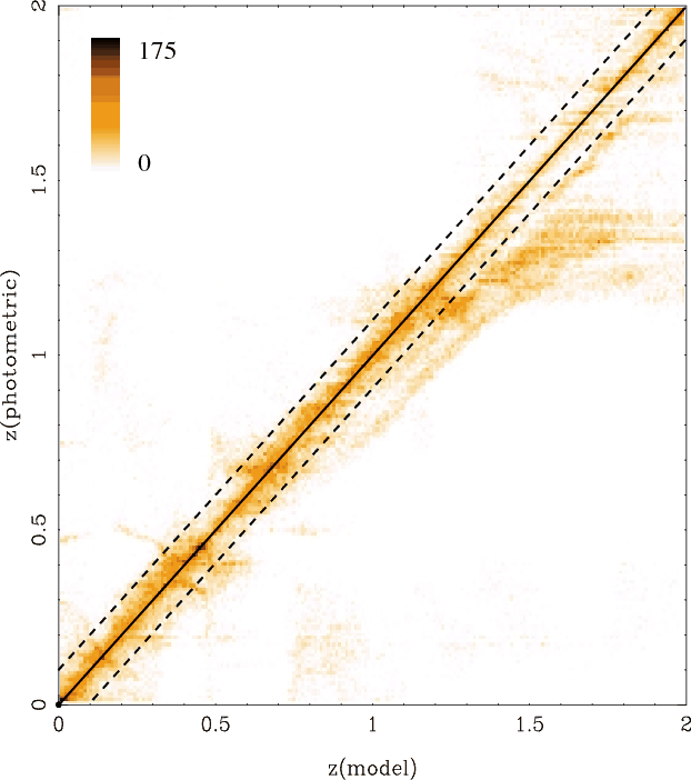
Figure 1:
Photometric versus model redshifts retrieved from
|
| Open with DEXTER | |
|
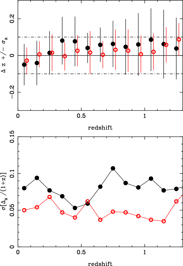
Figure 2:
Photometric versus model redshifts retrieved from
|
| Open with DEXTER | |
|
Figure 3:
These figures present the expected
|
| Open with DEXTER | |
Some systematic trends are clearly visible in Figs. 1-3.
The high-z filter combination provides a higher quality and smaller
systematic deviations than the low-z one. This trend was expected
because of the more complete and contiguous spectral coverage of the
high-z set. The lack of an R filter for the low-z sample introduces a
systematic trend in ![]()
![]() 0.05-0.08 at
0.05-0.08 at ![]() ;
the highest
;
the highest
![]() quality for this sample is expected to be around
quality for this sample is expected to be around
![]() at
at
![]() ,
i.e. within the sensitive redshift domain. Because of the lack
of B-band photometry for the high-z sample, the highest quality
results are expected at
,
i.e. within the sensitive redshift domain. Because of the lack
of B-band photometry for the high-z sample, the highest quality
results are expected at ![]() .
This trend is indeed
observed in the simulations.
However, the quality achived for high-zsimulated data at
.
This trend is indeed
observed in the simulations.
However, the quality achived for high-zsimulated data at ![]() with Hyperz
is expected to be overestimated
with respect to real data, because templates and models are drawn from
the same parent set. This is a general criticism of simulations used
in assessing the realistic performance of
with Hyperz
is expected to be overestimated
with respect to real data, because templates and models are drawn from
the same parent set. This is a general criticism of simulations used
in assessing the realistic performance of
![]() quality. Also
quality. Also
![]() quality depends on the spectral type of galaxies. With respect to the
average quality presented in Fig. 3 for a uniform
distribution of types, early types exhibit up to a
quality depends on the spectral type of galaxies. With respect to the
average quality presented in Fig. 3 for a uniform
distribution of types, early types exhibit up to a ![]() 50%
improvement in
50%
improvement in
![]() with Hyperz
in the redshift domains where the filter sets bracket the 4000 Å break.
with Hyperz
in the redshift domains where the filter sets bracket the 4000 Å break.
The results for the GR code in Table 9 are similar in
average to Hyperz's ones. The quality tend to be slightly better for the
bluest spectral types, whereas it is worse for early types. This trend can
be explained by the broad paramer space spanned by the simulations, the same
used by Hyperz for
![]() determinations, as compared to the GR code. The noise for late-type galaxies in Hyperz tend to be dominated by
degeneracies, whereas the GR code cannot properly fit highly-reddened
E-Sbc galaxies. Note that the uniform distribution in redshift and types in
these simulations does not represent a realistic population of galaxies.
determinations, as compared to the GR code. The noise for late-type galaxies in Hyperz tend to be dominated by
degeneracies, whereas the GR code cannot properly fit highly-reddened
E-Sbc galaxies. Note that the uniform distribution in redshift and types in
these simulations does not represent a realistic population of galaxies.
4.2 Comparison with spectroscopic redshifts
The
![]() accuracy achieved for EDisCS was estimated by direct
comparison with its 1449 spectroscopic redshifts in the
accuracy achieved for EDisCS was estimated by direct
comparison with its 1449 spectroscopic redshifts in the
![]() interval
(type 1+2).
Although
spectroscopic targets in our sample were strongly biased in favor of
cluster members with
interval
(type 1+2).
Although
spectroscopic targets in our sample were strongly biased in favor of
cluster members with
![]() within the interval
within the interval
![]() (see Halliday et al. 2004; Milvang-Jensen et al. 2008, and
Sect. 5.1), the geometrical configuration of slits in one
hand, and the need for reference field galaxies on the other hand,
ensured that non-member galaxies were also targeted during the
spectroscopic runs. In principle, these field galaxies should allow us
to extend the present study to the 0
(see Halliday et al. 2004; Milvang-Jensen et al. 2008, and
Sect. 5.1), the geometrical configuration of slits in one
hand, and the need for reference field galaxies on the other hand,
ensured that non-member galaxies were also targeted during the
spectroscopic runs. In principle, these field galaxies should allow us
to extend the present study to the 0 ![]()
![]()
![]() 1 interval,
according to the restrictions imposed by the set of filters (see
Sect. 4.1).
1 interval,
according to the restrictions imposed by the set of filters (see
Sect. 4.1).
Table 3 presents the
![]() accuracy obtained with Hyperz
and Rudnick's (GR) code for the different low-z and high-zclusters, based on the direct comparison with the spectroscopic
sample, excluding stars. Only type 1 objects, i.e. objects with
secure spectroscopic redshifts, were taken into account. In
Table 3, systematic deviations and
accuracy obtained with Hyperz
and Rudnick's (GR) code for the different low-z and high-zclusters, based on the direct comparison with the spectroscopic
sample, excluding stars. Only type 1 objects, i.e. objects with
secure spectroscopic redshifts, were taken into account. In
Table 3, systematic deviations and ![]() were computed
over all the
were computed
over all the
![]() interval. In the low-z bin,
the two clusters with only BVI photometry were excluded from the
sample when computing the average
interval. In the low-z bin,
the two clusters with only BVI photometry were excluded from the
sample when computing the average
![]() quality over the cluster
sample. In the high-z bin, we excluded Cl1122-1136 from the cluster
statistics, because of the small number of
quality over the cluster
sample. In the high-z bin, we excluded Cl1122-1136 from the cluster
statistics, because of the small number of
![]() available in this
field.
available in this
field.
Our main result is that there is no significant systematic
shift, neither in the
![]() nor in the
nor in the
![]() results, with respect to the values expected
from simulations in Sect. 4.1, with some field-to-field
differences discussed below. The accuracy of
results, with respect to the values expected
from simulations in Sect. 4.1, with some field-to-field
differences discussed below. The accuracy of
![]() ranges usually
between
ranges usually
between
![]() for Hyperz and
for Hyperz and
![]() 0.06 for GR, both for the low-z and the high-z samples. This
result is in good agreement with the highest possible accuracy
expected from ideal simulations in the low-z case,
it is
0.06 for GR, both for the low-z and the high-z samples. This
result is in good agreement with the highest possible accuracy
expected from ideal simulations in the low-z case,
it is ![]() 25% worse than ideal expectations in the high-z case
for Hyperz, and compatible with GR results for late type galaxies
(early-type errors were overestimated, as mentioned in Sect. 4.1).
The differential trend between low and high-z samples with respect to
simulations in both codes
can be explained because of the different population of
``bright'' galaxies in these fields, low-z and high-z samples
containing a smaller and larger fraction of late-type galaxies
respectively, compared to the uniform average population in simulated
data (e.g. De Lucia et al. 2007). This effect is clearly seen in
Table 4.
The fraction of objects lost from (or spuriously assigned to) the
relevant redshift interval according to the definitions given above
(
25% worse than ideal expectations in the high-z case
for Hyperz, and compatible with GR results for late type galaxies
(early-type errors were overestimated, as mentioned in Sect. 4.1).
The differential trend between low and high-z samples with respect to
simulations in both codes
can be explained because of the different population of
``bright'' galaxies in these fields, low-z and high-z samples
containing a smaller and larger fraction of late-type galaxies
respectively, compared to the uniform average population in simulated
data (e.g. De Lucia et al. 2007). This effect is clearly seen in
Table 4.
The fraction of objects lost from (or spuriously assigned to) the
relevant redshift interval according to the definitions given above
(![]() and
and ![]() ), is negligible in the low-z sample and typically
below 5% for the high-z one.
), is negligible in the low-z sample and typically
below 5% for the high-z one.
Table 4 summarizes the results obtained for the entire low-zand high-z samples, for both type 1 (secure) and type 1 + type 2
(both secure and slightly tentative redshifts) spectroscopic data.
The results are similar in both cases. In the high-z bin,
![]() accuracy improves slightly when the sample is restricted to the
accuracy improves slightly when the sample is restricted to the
![]() interval, where both Hyperz and GR codes
yield the same
interval, where both Hyperz and GR codes
yield the same
![]() .
This effect is
easily understood because at
.
This effect is
easily understood because at
![]() the rest-frame
4000 Å break is found shortward of the V-band filter.
Table 4 also summarizes the
the rest-frame
4000 Å break is found shortward of the V-band filter.
Table 4 also summarizes the
![]() accuracy achieved for the
different spectral types of galaxies in the entire sample,
i.e. all type 1, 2 and 3 spectra. Tentative type 3 galaxies
represent less than 2% of the total sample, and the results remain unchanged
whith respect to type 1+2. The number of galaxies as a function of the
spectral type given in this table correspond to Hyperz. Excepted for
catastrophic identifications, the classification obtained with the two codes
is in perfect agreement.
The lowest
quality
accuracy achieved for the
different spectral types of galaxies in the entire sample,
i.e. all type 1, 2 and 3 spectra. Tentative type 3 galaxies
represent less than 2% of the total sample, and the results remain unchanged
whith respect to type 1+2. The number of galaxies as a function of the
spectral type given in this table correspond to Hyperz. Excepted for
catastrophic identifications, the classification obtained with the two codes
is in perfect agreement.
The lowest
quality
![]() values are measured as expected for
the bluest galaxy types (SB), for both the Hyperz and GR
codes. Early types display the highest quality results with Hyperz, whereas GR code has lower quality results for early types
in the high-z sample. This trend may indicate that the CWW templates
provide an inappropriate description of the SEDs of early types at
intermediate redshifts.
values are measured as expected for
the bluest galaxy types (SB), for both the Hyperz and GR
codes. Early types display the highest quality results with Hyperz, whereas GR code has lower quality results for early types
in the high-z sample. This trend may indicate that the CWW templates
provide an inappropriate description of the SEDs of early types at
intermediate redshifts.
The comparison between the Hyperz and GR codes, either on a
cluster-by-cluster basis or as a function of the filter combination,
yields similar results, even though these codes are based on different
approaches and have different strengths/weaknesses. In general, Hyperz results are found to be of slightly higher accuracy than
GR's ones (by ![]() 20% in
20% in
![]() ), but both
are in close agreement with the expectations under ``ideal''
conditions. An interesting trend is that the quality of both codes is
highly correlated, in the sense that the highest and the lowest
quality results (in terms of
), but both
are in close agreement with the expectations under ``ideal''
conditions. An interesting trend is that the quality of both codes is
highly correlated, in the sense that the highest and the lowest
quality results (in terms of
![]() and systematics)
are found for the same clusters. Given the homogeneous photometry of
the EDisCS project, this trend can hardly be explained by the use of
an incomplete or imperfect template set (as suggested by
Ilbert et al. 2006), because in such a case we would expect the same
systematic behavior in all fields, given a certain filter set, as is
observed in Sect. 4.1 with Hyperz. In contrast, different
systematic trends are observed for different clusters, which are then
found to be almost identical for the two independent
and systematics)
are found for the same clusters. Given the homogeneous photometry of
the EDisCS project, this trend can hardly be explained by the use of
an incomplete or imperfect template set (as suggested by
Ilbert et al. 2006), because in such a case we would expect the same
systematic behavior in all fields, given a certain filter set, as is
observed in Sect. 4.1 with Hyperz. In contrast, different
systematic trends are observed for different clusters, which are then
found to be almost identical for the two independent
![]() codes. This behavior suggests strongly that the origin of the
systematics is more likely to be the input photometric catalog rather
than the
codes. This behavior suggests strongly that the origin of the
systematics is more likely to be the input photometric catalog rather
than the
![]() codes and templates. In particular, we cannot exclude
small remaining zero-point shifts in our data, approximately equal to
or less than
codes and templates. In particular, we cannot exclude
small remaining zero-point shifts in our data, approximately equal to
or less than ![]() 0.05 mag, because we are limited by the
accuracy of the stellar templates (see Sect. 2).
0.05 mag, because we are limited by the
accuracy of the stellar templates (see Sect. 2).
A brief discussion of particular aspects of
![]() accuracy in the
low-z and high-z samples is given below.
accuracy in the
low-z and high-z samples is given below.
4.2.1 Low-z cluster fields
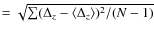
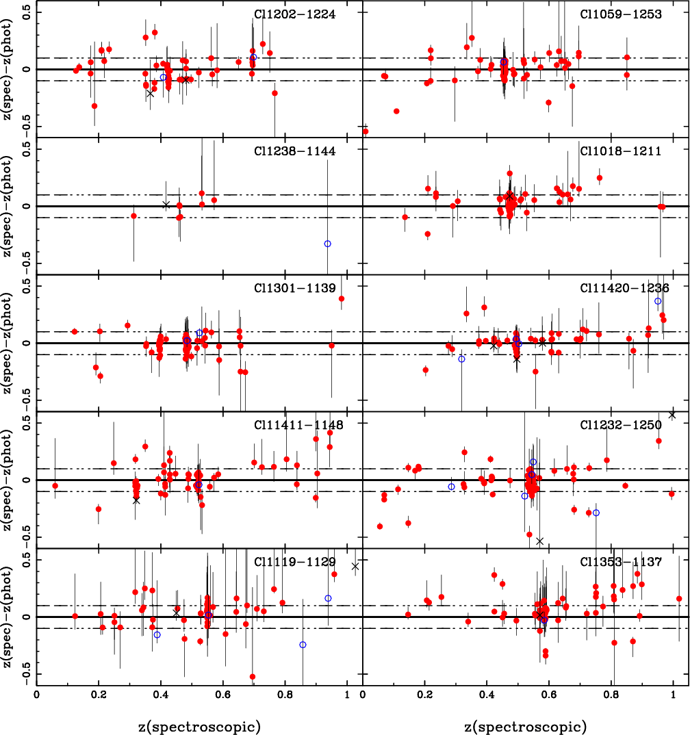
Figure 4 displays a direct comparison between the
spectroscopic and the photometric redshifts for the low-z clusters in
the EDisCS sample. Hyperz was used to derive
![]() in this
figure, but the results with the GR code are very similar, as
discussed above. Error bars in
in this
figure, but the results with the GR code are very similar, as
discussed above. Error bars in
![]() correspond to a 1
correspond to a 1![]() confidence level in the photometric redshift probability distribution
P(z), i.e. to the 68% confidence level computed through the
confidence level in the photometric redshift probability distribution
P(z), i.e. to the 68% confidence level computed through the
![]() increment for a single parameter (Avni 1976).
Figure 16 shows the comparison between spectroscopic and
photometric redshifts for the entire low-z sample, obtained with
Hyperz and GR codes, as well as the
increment for a single parameter (Avni 1976).
Figure 16 shows the comparison between spectroscopic and
photometric redshifts for the entire low-z sample, obtained with
Hyperz and GR codes, as well as the
![]() distribution.
distribution.
The
![]() quality in this sample ranges usually between
quality in this sample ranges usually between
![]() with both Hyperz and GR codes, with some exceptions. On the one hand,
Cl1119-1129 and Cl1238-1144 were only observed in BVI, which produces
lower quality
with both Hyperz and GR codes, with some exceptions. On the one hand,
Cl1119-1129 and Cl1238-1144 were only observed in BVI, which produces
lower quality
![]() and a higher fraction of catastrophic
identifications.
These two clusters were not included when deriving
the mean values in Table 3.
On the other hand, Cl1232-1250
was observed in J in addition to BVIK, and this provides a more
accurate
and a higher fraction of catastrophic
identifications.
These two clusters were not included when deriving
the mean values in Table 3.
On the other hand, Cl1232-1250
was observed in J in addition to BVIK, and this provides a more
accurate
![]() estimate with respect to average
with Hyperz, although there is no clear improvement with the GR code.
Compared to simulations, the systematic trend
estimate with respect to average
with Hyperz, although there is no clear improvement with the GR code.
Compared to simulations, the systematic trend
![]() -0.08 at
-0.08 at ![]() is far smaller in real data, whereas
is far smaller in real data, whereas
![]() is in agreement with ideal results.
is in agreement with ideal results.
Table 1:
![]() accuracy from simulations
for galaxies in the spectroscopic sample, based on Hyperz.
accuracy from simulations
for galaxies in the spectroscopic sample, based on Hyperz.
Table 2:
![]() accuracy expected for the faintest galaxies in the
EDisCS sample, in the low-z and high-z fields, based on Hyperz.
accuracy expected for the faintest galaxies in the
EDisCS sample, in the low-z and high-z fields, based on Hyperz.
4.2.2 High-z cluster fields
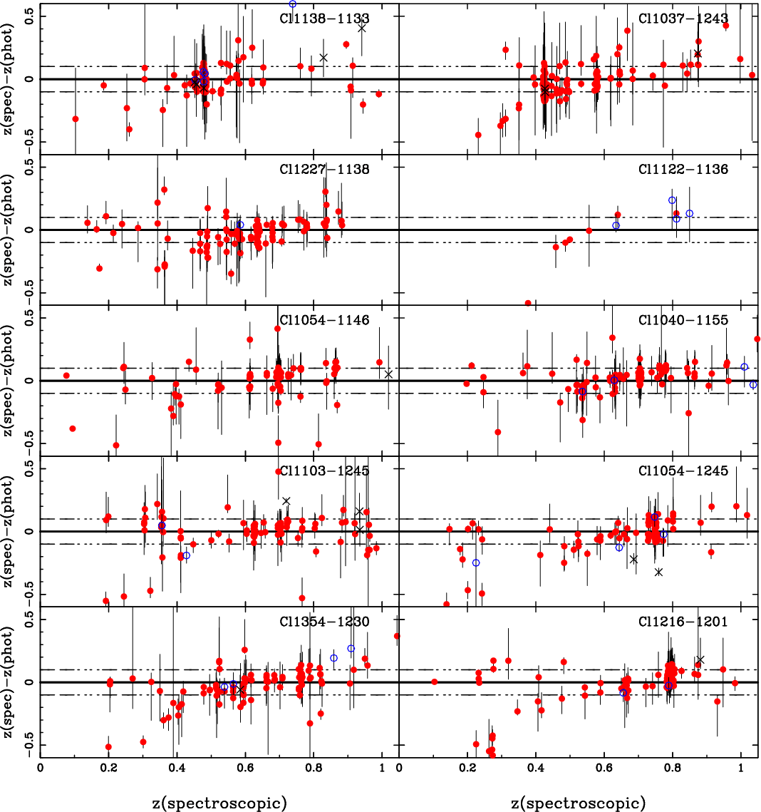
Figure 5 displays a direct comparison between the
spectroscopic and the photometric redshifts for the high-z clusters in
the EDisCS sample. Error bars in
![]() correspond to 1
correspond to 1![]() confidence level in the photometric redshift probability distribution
P(z).
Figure 17 shows the comparison between spectroscopic and
photometric redshifts for the whole high-z sample, obtained with
Hyperz and GR codes, as well as the
confidence level in the photometric redshift probability distribution
P(z).
Figure 17 shows the comparison between spectroscopic and
photometric redshifts for the whole high-z sample, obtained with
Hyperz and GR codes, as well as the
![]() distribution.
distribution.
The
![]() quality in this sample usually ranges between
quality in this sample usually ranges between
![]() with both Hyperz and GR codes, with some exceptions. The statistics in
Cl1122-1136 is based on a small number of spectroscopic redshifts,
hence we exclude this cluster when deriving the mean values in
Table 4.
Two out of the ten clusters in the high-z sample are actually
in a redshift range typical of the low-z sample. Indeed,
in the case of
Cl1037-1243a
and Cl1138-1133, the low redshift of the
cluster implies that B-band photometry is required to ensure that an
accurate
with both Hyperz and GR codes, with some exceptions. The statistics in
Cl1122-1136 is based on a small number of spectroscopic redshifts,
hence we exclude this cluster when deriving the mean values in
Table 4.
Two out of the ten clusters in the high-z sample are actually
in a redshift range typical of the low-z sample. Indeed,
in the case of
Cl1037-1243a
and Cl1138-1133, the low redshift of the
cluster implies that B-band photometry is required to ensure that an
accurate
![]() measurement is achieved, although the quality of their
measurement is achieved, although the quality of their
![]() measurements is close to average. As seen in
Fig. 5, individual error bars are larger in these two
fields than in the other high-z clusters. Compared to simulations,
there is no systematic trend in
measurements is close to average. As seen in
Fig. 5, individual error bars are larger in these two
fields than in the other high-z clusters. Compared to simulations,
there is no systematic trend in ![]() as expected, whereas
as expected, whereas
![]() is in agreement with ideal results.
is in agreement with ideal results.
Table 3:
Summary of
![]() accuracy achieved for the
individual low-z and high-z clusters.
accuracy achieved for the
individual low-z and high-z clusters.
Table 4:
Summary of
![]() accuracy achieved for the
whole low-z and high-z samples with Hyperz and GR codes.
accuracy achieved for the
whole low-z and high-z samples with Hyperz and GR codes.
4.3 Expected accuracy for galaxies fainter than the spectroscopic sample
We determine the
![]() accuracy expected for galaxies fainter than
the spectroscopic control sample used in Sect. 4.2,
i.e. galaxies with magnitudes typically ranging between I=18.5(19.0)
and 22.0 in the low-z (high-z) sample, in particular for the faintest
galaxies in the EDisCS sample. The concept is to derive
accuracy expected for galaxies fainter than
the spectroscopic control sample used in Sect. 4.2,
i.e. galaxies with magnitudes typically ranging between I=18.5(19.0)
and 22.0 in the low-z (high-z) sample, in particular for the faintest
galaxies in the EDisCS sample. The concept is to derive
![]() on a
degraded version of the photometric catalog for the spectroscopic
sample (in terms of S/N), using the same recipes and settings as the
main catalogs. This method was preferred instead of simulations
because it uses the observed SEDs of the control sample instead of an
arbitrary mixture of spectral types at a given redshift.
on a
degraded version of the photometric catalog for the spectroscopic
sample (in terms of S/N), using the same recipes and settings as the
main catalogs. This method was preferred instead of simulations
because it uses the observed SEDs of the control sample instead of an
arbitrary mixture of spectral types at a given redshift.
Degradated catalogs were generated from the original (spectroscopic)
ones, to reproduce the photometric properties of the faintest galaxies
in the EDisCS sample. The mean I magnitude was set to be
![]() (24.5) for the low-z(high-z) cluster fields, corresponding
to a
(24.5) for the low-z(high-z) cluster fields, corresponding
to a
![]() .
For all the other j filters, magnitudes were
scaled according to the original SEDs, i.e. keeping colors unchanged:
.
For all the other j filters, magnitudes were
scaled according to the original SEDs, i.e. keeping colors unchanged:
![]() Photometric errors as a function of apparent magnitudes were
introduced and assigned as in Sect. 4.1. In this case,
Photometric errors as a function of apparent magnitudes were
introduced and assigned as in Sect. 4.1. In this case,
![]() ,
where
,
where
![]() is the catalog error corresponding to m(j), and
is the catalog error corresponding to m(j), and
![]() .
This procedure conserves
globally the colors of galaxies. The main caveat is the fact that this
noisy population does not necessarily match the true color
distribution of the faintest galaxies in the sample. However, it is
useful to estimate the degradation expected in
.
This procedure conserves
globally the colors of galaxies. The main caveat is the fact that this
noisy population does not necessarily match the true color
distribution of the faintest galaxies in the sample. However, it is
useful to estimate the degradation expected in
![]() accuracy between
the brightest and the faintest galaxies because of the lowered S/N.
Because
accuracy between
the brightest and the faintest galaxies because of the lowered S/N.
Because
![]() quality is quite insensitive to spectroscopic quality,
we added the type 1 + type 2 spectroscopic catalogs.
quality is quite insensitive to spectroscopic quality,
we added the type 1 + type 2 spectroscopic catalogs.
Table 2 and 10 summarize the results
obtained for the faintest galaxies using Hyperz and the GR code
respectively. These tables can be compared directly with Table 4.
The quality of photometric redshifts degrades typically by a factor of
two in
![]() between the brightest (
between the brightest (![]() )
and the faintest (
)
and the faintest (![]() -24.5) galaxies in the EDisCS sample. Most
of the trends observed in Table 4 for the spectroscopic
sample are found in the
Table 2 for the simulations of the faintest sample,
in particular
the lack of systematics in
-24.5) galaxies in the EDisCS sample. Most
of the trends observed in Table 4 for the spectroscopic
sample are found in the
Table 2 for the simulations of the faintest sample,
in particular
the lack of systematics in ![]() ,
and the higher quality results
in the high-z bin. The fraction of catastrophic identifications
increases, but remains typically below
,
and the higher quality results
in the high-z bin. The fraction of catastrophic identifications
increases, but remains typically below ![]() 5%. The difference in
5%. The difference in
![]() quality between early and late types is smaller for the
faintest galaxy sample.
In this case, the simulation results with the GR code are found to be of
slightly higher accuracy than Hyperz's ones (by
quality between early and late types is smaller for the
faintest galaxy sample.
In this case, the simulation results with the GR code are found to be of
slightly higher accuracy than Hyperz's ones (by ![]() 20% in
20% in
![]() ).
In Sect. 6.3, we comment on the
implications that this results will have for the calculation of
membership using the photometric redshifts.
).
In Sect. 6.3, we comment on the
implications that this results will have for the calculation of
membership using the photometric redshifts.
5 Photometric determination of cluster redshifts
5.1 Spectroscopic sample preselection
Before the first spectroscopic runs, cluster redshifts were estimated
from the first
![]() catalogs using Hyperz. Spectroscopic
targets were selected mainly to have
catalogs using Hyperz. Spectroscopic
targets were selected mainly to have
![]() within the interval
within the interval
![]() ,
or
absolute
,
or
absolute
![]()
![]() 0.5,
and according to the magnitude selection (see Halliday et al. 2004).
Although the results discussed in this section were obtained with Hyperz, they should be representative of the general behavior of
all SED-fitting
0.5,
and according to the magnitude selection (see Halliday et al. 2004).
Although the results discussed in this section were obtained with Hyperz, they should be representative of the general behavior of
all SED-fitting
![]() codes.
codes.
Table 5:
Comparison between spectroscopic (
![]() )
and photometric
determinations of cluster redshifts in the low and high-z samples.
)
and photometric
determinations of cluster redshifts in the low and high-z samples.
The photometic cluster redshifts were computed from the photometric
redshift distribution by comparing the N(z) obtained in the center of
the field with the equivalent one over a wider region of the same
area, obtained under the same conditions from the
![]() point of view
(same effective exposure time and number of filters), and used as a
blank field. A real cluster or other structure should have appeared as
an excess of galaxies in the central region in comparison to the outer
parts. In this exercise, we considered only objects with
point of view
(same effective exposure time and number of filters), and used as a
blank field. A real cluster or other structure should have appeared as
an excess of galaxies in the central region in comparison to the outer
parts. In this exercise, we considered only objects with ![]() i.e. objects that could not be excluded as galaxies without applying a
cut in magnitude. Figure 6 displays the results found for the
different fields.The histograms in this Figure display the difference
between the redshift distribution within a
i.e. objects that could not be excluded as galaxies without applying a
cut in magnitude. Figure 6 displays the results found for the
different fields.The histograms in this Figure display the difference
between the redshift distribution within a ![]() 140
140
![]() radius region
centered on the center of the image (
radius region
centered on the center of the image (
![]() ,
black solid line),
and the distribution within an outer ring,
,
black solid line),
and the distribution within an outer ring,
![]() ,
(
,
(
![]() ,
dashed black lines). Red solid lines show the positive
difference between the two histograms,
,
dashed black lines). Red solid lines show the positive
difference between the two histograms,
![]() .
Histograms were obtained with a
.
Histograms were obtained with a
![]() sampling step and
smoothed with a
sampling step and
smoothed with a
![]() sliding window. This window
corresponded approximately to the
sliding window. This window
corresponded approximately to the ![]() uncertainty in the
uncertainty in the
![]() estimate for the faintest galaxies in the catalog.
estimate for the faintest galaxies in the catalog.
Where there was a distinct peak in
![]() distribution, we used this value to represent the
``cluster redshift''. We also computed 2D number density maps and cluster
tomography (see Sect. 5.3 below) to emphasize the reality of
the clusters, in particular for the uncertain cases. A summary of
these results was provided in White et al. (2005). We note that the
efficiency of the cluster-finding algorithm could be enhanced if the
central region was centered on the cluster centroid instead of the
center of the image. This ideal situation could be achieved in wider
surveys.
distribution, we used this value to represent the
``cluster redshift''. We also computed 2D number density maps and cluster
tomography (see Sect. 5.3 below) to emphasize the reality of
the clusters, in particular for the uncertain cases. A summary of
these results was provided in White et al. (2005). We note that the
efficiency of the cluster-finding algorithm could be enhanced if the
central region was centered on the cluster centroid instead of the
center of the image. This ideal situation could be achieved in wider
surveys.
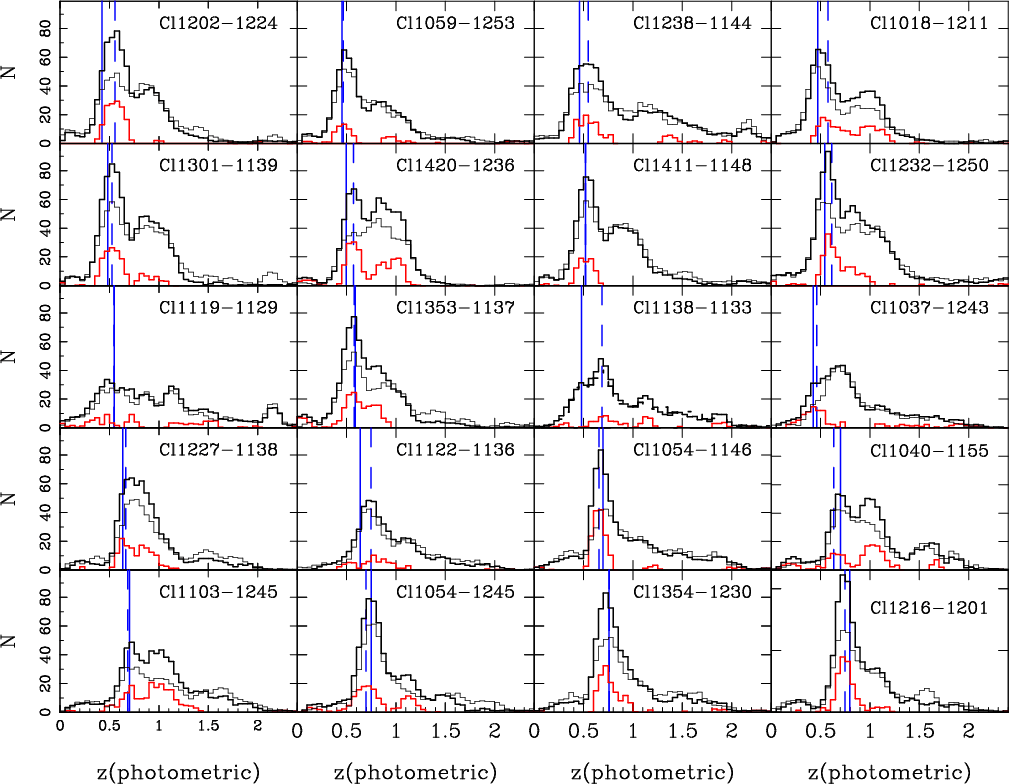
|
Figure 4:
(
|
| Open with DEXTER | |
|
Figure 5:
(
|
| Open with DEXTER | |
|
Figure 6:
Photometric redshift distributions in the EDisCS fields,
with the cluster redshift increasing from top to bottom and from
left to right,
for the low-z and high-z samples (first and second series respectively).
The histograms display the following redshift
distributions:
|
| Open with DEXTER | |
5.2 Spectroscopic versus photometric cluster redshifts
Figure 6 summarizes the comparison between the
![]() and
spectroscopic redshifts for the different cluster fields.
The photometric cluster redshift can be defined in different
ways. Here we have adopted two different definitions, which are
reported in Table 5: (1) the mean weighted value,
computed from the excess peak, and (2) the redshift corresponding to
the maximum value in the
and
spectroscopic redshifts for the different cluster fields.
The photometric cluster redshift can be defined in different
ways. Here we have adopted two different definitions, which are
reported in Table 5: (1) the mean weighted value,
computed from the excess peak, and (2) the redshift corresponding to
the maximum value in the
![]() histogram.
Table 5 provides a comparison between spectroscopic and
photometric determinations of cluster redshifts for the low and high-zsamples. Cluster redshifts in Table 5 and
Fig. 6 correspond to
the most prominent cluster identification
when several clusters were present in the field (Milvang-Jensen et al. 2008). Five fields were excluded when computing the systematic
deviation and dispersion: Cl1119-1129 and Cl1238-1144 in the low-zsample, because of incomplete photometry; and Cl1122-1136,
Cl1037-1243a and Cl1138-1133
in the high-z sample, the first because of the
lack of a clear cluster in the field, and the two others because their
low cluster redshifts implied that B-band photometry was required to
achieve an accurate
histogram.
Table 5 provides a comparison between spectroscopic and
photometric determinations of cluster redshifts for the low and high-zsamples. Cluster redshifts in Table 5 and
Fig. 6 correspond to
the most prominent cluster identification
when several clusters were present in the field (Milvang-Jensen et al. 2008). Five fields were excluded when computing the systematic
deviation and dispersion: Cl1119-1129 and Cl1238-1144 in the low-zsample, because of incomplete photometry; and Cl1122-1136,
Cl1037-1243a and Cl1138-1133
in the high-z sample, the first because of the
lack of a clear cluster in the field, and the two others because their
low cluster redshifts implied that B-band photometry was required to
achieve an accurate
![]() (see also Milvang-Jensen et al. 2008). We
note however the accurate photometric identification of the Cl1037-1243a cluster,
for which a poor determination was expected.
(see also Milvang-Jensen et al. 2008). We
note however the accurate photometric identification of the Cl1037-1243a cluster,
for which a poor determination was expected.
In general, the differences between photometric and spectroscopic
values are small, ranging from
![]() -0.04 at high-z to
-0.04 at high-z to
![]() at low-z. The dispersion is much lower than the
approximate cut introduced by the spectroscopic preselection
(
at low-z. The dispersion is much lower than the
approximate cut introduced by the spectroscopic preselection
(
![]() ). Therefore, there is no reason why a cluster
should have been ``missed'' within the relevant redshift interval due
to
). Therefore, there is no reason why a cluster
should have been ``missed'' within the relevant redshift interval due
to
![]() preselection. The systematic trend of lower quality in
preselection. The systematic trend of lower quality in
![]() for the low-z sample was expected from the simulations
presented in Sect. 4.1, and also observed in the comparison with
the spectroscopic sample in Sect. 4.2.
for the low-z sample was expected from the simulations
presented in Sect. 4.1, and also observed in the comparison with
the spectroscopic sample in Sect. 4.2.
5.3 Cluster tomography
We present results about cluster tomography along the line-of-sight in
the different EDisCS fields. This highlights the capability of
![]() in identifying and studying clusters of galaxies in deep photometric
surveys.
in identifying and studying clusters of galaxies in deep photometric
surveys.
A local density estimate was derived at each point in the field
using a grid with
![]()
![]() .
The density estimator was defined,
according to the formalism introduced by Dressler (1980), to equal
.
The density estimator was defined,
according to the formalism introduced by Dressler (1980), to equal
![]() ,
where d20 was the projected
linear distance to the 20th closest neighbor. Photometric redshift
slices of
,
where d20 was the projected
linear distance to the 20th closest neighbor. Photometric redshift
slices of
![]() were used to cover the redshift range
were used to cover the redshift range
![]() .
Close neighbors were selected within
.
Close neighbors were selected within
![]()
![]() 0.1,
centered on the redshift bin. The arbitrary choices of
0.1,
centered on the redshift bin. The arbitrary choices of ![]() and
n=20 were justified by the typical richnesses of clusters and the
and
n=20 were justified by the typical richnesses of clusters and the
![]() accuracy.
We tested other values of n ranging between 5 and 20 and achieved
similar results for the cluster detection. Edge effects
were corrected by using external fields in the main eight directions
(i.e. X+, Y+, X-, Y-, X+Y+, X+Y-, X-Y+, X-Y-),
containing different realizations of the same
accuracy.
We tested other values of n ranging between 5 and 20 and achieved
similar results for the cluster detection. Edge effects
were corrected by using external fields in the main eight directions
(i.e. X+, Y+, X-, Y-, X+Y+, X+Y-, X-Y+, X-Y-),
containing different realizations of the same
![]() slice with xycoordinates randomly sorted. The density maps were smoothed with a
Gaussian kernel of
slice with xycoordinates randomly sorted. The density maps were smoothed with a
Gaussian kernel of
![]() .
.
Figures 7 and 8 display the projected
number density maps obtained with this method, for the low and high-zsamples, respectively. In these figures, clusters are presented with
![]() increasing from top to bottom. Projected number
densities are displayed on a linear scale, for an arbitrary redshift
step
increasing from top to bottom. Projected number
densities are displayed on a linear scale, for an arbitrary redshift
step
![]() ,
with isopleths corresponding to increasing number
density bins, equally spaced
with
,
with isopleths corresponding to increasing number
density bins, equally spaced
with
![]() ,
starting at
the mean
,
starting at
the mean
![]() within the redshift slice. The presence of a
cluster along the line-of-sight is clearly seen in most cases, at
least in all cases where a cluster was clearly detected in the
field. We note that the
within the redshift slice. The presence of a
cluster along the line-of-sight is clearly seen in most cases, at
least in all cases where a cluster was clearly detected in the
field. We note that the
![]() value is affected by the
presence of a cluster in the corresponding redshift bin. The most
significant contrast in the density map is found usually for the
value is affected by the
presence of a cluster in the corresponding redshift bin. The most
significant contrast in the density map is found usually for the
![]() redshift slice (rightmost column of
Figs. 7 and 8). The position of the BCG
(White et al. 2005; Milvang-Jensen et al. 2008;
Whiley et al. 2008;
displayed by a blue cross in these figures)
coincides usually with the maximum contrast in the density map
for the most prominent clusters in a given field. The
comparison between this maximum-contrast slice and the tomography with
fixed arbitrary step (e.g.
redshift slice (rightmost column of
Figs. 7 and 8). The position of the BCG
(White et al. 2005; Milvang-Jensen et al. 2008;
Whiley et al. 2008;
displayed by a blue cross in these figures)
coincides usually with the maximum contrast in the density map
for the most prominent clusters in a given field. The
comparison between this maximum-contrast slice and the tomography with
fixed arbitrary step (e.g.
![]() ,
the step used in
Figs. 7 and 8) suggests that the optimal
redshift step for detection of clusters along the line-of-sight should
be close to the typical difference between photometric and
spectroscopic
,
the step used in
Figs. 7 and 8) suggests that the optimal
redshift step for detection of clusters along the line-of-sight should
be close to the typical difference between photometric and
spectroscopic
![]() ,
in this case
,
in this case
![]() .
Structures separated by less than
.
Structures separated by less than
![]() in
redshift space cannot be distinguished by
in
redshift space cannot be distinguished by
![]() tomography
(e.g. clusters Cl1138 (z=0.48) and Cl1138a (z=0.45) in the 1138.2-1133 field,
and Cl1227 (z=0.63) and Cl1227a (z=0.58) in the 1227.9-1138 field;
Milvang-Jensen et al. 2008).
tomography
(e.g. clusters Cl1138 (z=0.48) and Cl1138a (z=0.45) in the 1138.2-1133 field,
and Cl1227 (z=0.63) and Cl1227a (z=0.58) in the 1227.9-1138 field;
Milvang-Jensen et al. 2008).
For all clusters clearly identifiable in this sample (i.e. all
clusters except Cl1059-1253, Cl1202-1224 and Cl1119-1129), the maximum
contrast is found to be at least ![]()
![]() about
about
![]() .
All clusters in our sample exhibit a
significant
.
All clusters in our sample exhibit a
significant ![]()
![]() overdensity around
overdensity around
![]() ,
defined to be
,
defined to be
![]() ,
where
,
where ![]() represents the standard deviation in the projected number
density within the redshift bin. For all apart from the three
aforementioned clusters, the detection level exceeds
represents the standard deviation in the projected number
density within the redshift bin. For all apart from the three
aforementioned clusters, the detection level exceeds ![]() ,
and
ranges between 6 and
,
and
ranges between 6 and ![]() for Cl1216-1201, Cl1227-1138,
Cl1411-1148, Cl1420-1236, Cl1040-1155, Cl1054-1245, Cl1138-1133,
Cl1018-1211, and Cl1054-1146.
No other significant overdensities are found along the line-of-sight
of density peaks exceeding
for Cl1216-1201, Cl1227-1138,
Cl1411-1148, Cl1420-1236, Cl1040-1155, Cl1054-1245, Cl1138-1133,
Cl1018-1211, and Cl1054-1146.
No other significant overdensities are found along the line-of-sight
of density peaks exceeding
![]() ,
which are typical values
for rich clusters in this sample. However, several overdensities are
found with slightly smaller values, around
,
which are typical values
for rich clusters in this sample. However, several overdensities are
found with slightly smaller values, around ![]()
![]() ,
and detection levels exceeding
,
and detection levels exceeding ![]() .
These structures are
identified by circles in Figs. 7 and 8 (see below). Their reliability is difficult to
assess with the presently available data.
.
These structures are
identified by circles in Figs. 7 and 8 (see below). Their reliability is difficult to
assess with the presently available data.
Several fields deserve further comment. More information concerning the spectroscopic identification of clusters in these fields can be found in the reference papers by Halliday et al. (2004) and Milvang-Jensen et al. (2008):
- Cl1301-1139: The two clusters identified in this field with
z(spectroscopic) = 0.397 (Cl1301a)
and 0.482 (Cl1301) are consistent with the two
different
 peaks observed by our
tomography.
peaks observed by our
tomography.
- Cl1037-1243: The most distinct

 overdensity in this field corresponds to the ``a'' component at
z(spectroscopic) = 0.425, whereas the first identification was given
at z(spectroscopic) = 0.578 (
overdensity in this field corresponds to the ``a'' component at
z(spectroscopic) = 0.425, whereas the first identification was given
at z(spectroscopic) = 0.578 (
 in
Fig. 8). Both structures are seen by tomography.
in
Fig. 8). Both structures are seen by tomography.
- Cl1354-1230: the two clusters Cl1354 and Cl1354a
(z=0.762 and
z=0.595 respectively) are consistent with overdensities at the

 level.
- Cl1103-1245: The prominent
cluster detected in this field at
z=0.96 is clearly visible (
 level) both in the
density map and the
distribution (Fig. 6).
The two components Cl1103a (z=0.626) and Cl1103b (z=0.703)
can hardly be separated by tomography.
level) both in the
density map and the
distribution (Fig. 6).
The two components Cl1103a (z=0.626) and Cl1103b (z=0.703)
can hardly be separated by tomography.
- Other secondary peaks at
 are seen in the
N(
) distribution of Cl1018-1211, Cl1301-1139, Cl1420-1236,
Cl1054-1245, and Cl1040-1155 (Fig. 6). All can be
associated with spatial overdensities of
are seen in the
N(
) distribution of Cl1018-1211, Cl1301-1139, Cl1420-1236,
Cl1054-1245, and Cl1040-1155 (Fig. 6). All can be
associated with spatial overdensities of
 at the
 level, apart from in the field of Cl1040-1155, where no
significant overdensity is found.
level, apart from in the field of Cl1040-1155, where no
significant overdensity is found.
- Several additional overdensities/structures at
 are found in Cl1411-1148, Cl1119-1129, Cl1238-1144, and Cl1216-1201,
with
and detection levels ranging between 4 and
6
are found in Cl1411-1148, Cl1119-1129, Cl1238-1144, and Cl1216-1201,
with
and detection levels ranging between 4 and
6 .
Given the limited photometric coverage of Cl1119-1129
and Cl1238-1144, the detected overdensities in these fields are
rather dubious.
.
Given the limited photometric coverage of Cl1119-1129
and Cl1238-1144, the detected overdensities in these fields are
rather dubious.
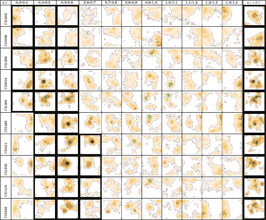
|
Figure 7:
Projected number density maps for the low-z sample, for
different redshift slices with
|
| Open with DEXTER | |
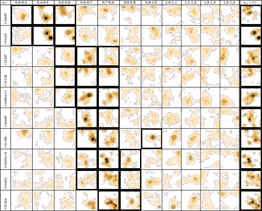
|
Figure 8: Projected number density maps for the high-z sample, for different redshift slices. Same comments as in Fig. 7. There is no clear BCG identified in Cl1122-1136. |
| Open with DEXTER | |
6 Cluster membership criteria
The most unambiguous way to determine cluster membership is by means of accurate spectroscopic redshifts. Unfortunately, it is far too time-consuming to obtain high spectroscopic completeness in cluster member observations, even to relatively bright limits of I< 22-23. For this reason, it is necessary to develop membership criteria that rely solely on photometric data. To achieve many EDisCS science goals, such as study of luminosity functions and cluster substructure, any method should: 1) retain >90% of cluster members; 2) reject an optimal number of non-members; and 3) measure a probability that a given galaxy is a cluster member. The first two criteria should be implemented so that there is little dependence on the galaxy color, e.g. for Butcher-Oemler-type studies. While traditional methods of statistical subtraction using ``field'' surveys of comparable depth offer a viable method to satisfy the first two criteria, they do not satisfy the third. For this reason, we developed an alternative method for membership determination based on our photometric redshifts estimates.
We present below how we use the photometric redshift probability distribution P(z) to reject non-members from each cluster field. We describe the method that we developed and its calibration based on EDisCS spectroscopic redshifts. We discuss how this method can be extended to the entire magnitude-limited sample for a given cluster and outline its limitations.
6.1 The method
Traditionally,
![]() -based methods for determining cluster membership
were based on a simple cut in redshift, such that a galaxy was
considered to be a member if
-based methods for determining cluster membership
were based on a simple cut in redshift, such that a galaxy was
considered to be a member if
![]() .
One disadvantage of this method is that
.
One disadvantage of this method is that
![]() can be as high as 0.3 (e.g. Toft et al. 2004), causing
considerable field contamination to enter into the cluster sample. An
additional disadvantage of the method is that it uses only the
best-fit redshift in determining membership and ignores the
information contained in the full redshift probability distribution
P(z).
can be as high as 0.3 (e.g. Toft et al. 2004), causing
considerable field contamination to enter into the cluster sample. An
additional disadvantage of the method is that it uses only the
best-fit redshift in determining membership and ignores the
information contained in the full redshift probability distribution
P(z).
Brunner & Lubin (2000) suggested an improved technique that used P(z)
in determining galaxy membership. They assumed a Gaussian P(z) of width
calculated from the comparison with
![]() ,
and defined the quantity
,
and defined the quantity
|
(1) |
where
6.2 Calibrating from the spectroscopic sample
We adopt the large and uniform EDisCS spectroscopic sample (Halliday
et al. 2004; Milvang-Jensen et al. 2008) to calibrate the
![]() that we use to reject non-members.
that we use to reject non-members.
We show in Figs. 9 and 10 the
![]() versus
versus
![]() -
-
![]() for all
galaxies with secure
for all
galaxies with secure
![]() measurements in our clusters, for the low and
high redshift samples, respectively. Results presented here were
obtained for the GR code, but they are similar for Hyperz.
As seen in Sect. 4, the
measurements in our clusters, for the low and
high redshift samples, respectively. Results presented here were
obtained for the GR code, but they are similar for Hyperz.
As seen in Sect. 4, the
![]() accuracy as well as the fraction of
catastrophic identifications in a given field depend on the spectral type of
galaxies, although the difference between early and late types is smaller for
the faintest galaxies in our sample. Therefore, we have studied the
reliability of the membership criteria for both early and late SED types
using a cut in the restframe color which splits the sample into two equal
halves of red (early) and blue (late) type galaxies. The color cuts are found to
be
accuracy as well as the fraction of
catastrophic identifications in a given field depend on the spectral type of
galaxies, although the difference between early and late types is smaller for
the faintest galaxies in our sample. Therefore, we have studied the
reliability of the membership criteria for both early and late SED types
using a cut in the restframe color which splits the sample into two equal
halves of red (early) and blue (late) type galaxies. The color cuts are found to
be
![]() = 0.79 and 0.67 for the low-z and high-z samples respectively.
The left and right-hand panels in Figs. 9 and 10 provide results for objects of different spectral
types.
= 0.79 and 0.67 for the low-z and high-z samples respectively.
The left and right-hand panels in Figs. 9 and 10 provide results for objects of different spectral
types.
We note that the ratio of members to non-members
increases as a function of
![]() .
There are also few galaxies with
.
There are also few galaxies with
![]()
![]()
![]() and very low
and very low
![]() values. This implies that there
are not many members that would be rejected because their faint
magnitudes correspond to broad P(z) and lead to their rejection even if
values. This implies that there
are not many members that would be rejected because their faint
magnitudes correspond to broad P(z) and lead to their rejection even if
![]()
![]()
![]() .
It is important to consider, however, that the
spectroscopic sample consists of the brightest galaxies of probably
the tightest P(z) values and that this behavior might not be similar at
fainter magnitudes (see Sect. 6.3).
.
It is important to consider, however, that the
spectroscopic sample consists of the brightest galaxies of probably
the tightest P(z) values and that this behavior might not be similar at
fainter magnitudes (see Sect. 6.3).
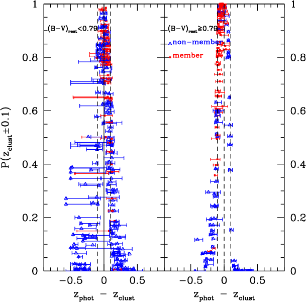
|
Figure 9:
The integrated probability of being at
|
| Open with DEXTER | |
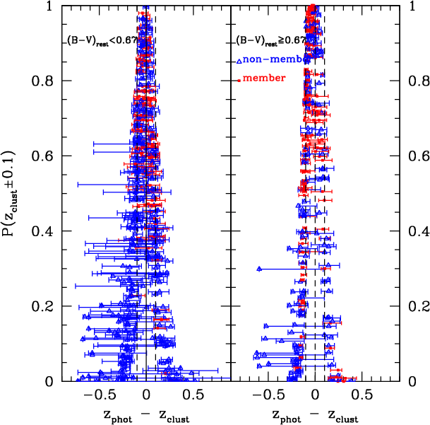
|
Figure 10: Same as Fig. 9 but for the high-z clusters. |
| Open with DEXTER | |
For the GR code, Figs. 11 and 12 demonstrate how the retained fraction of members
and rejected fraction of non-members depends on the
![]() threshold
threshold
![]() for the low-z and high-z samples, respectively. In both
cases, it is possible to define a
for the low-z and high-z samples, respectively. In both
cases, it is possible to define a
![]() value such that >90% of
confirmed cluster members are retained with little dependence on
rest-frame (or observed) color.
value such that >90% of
confirmed cluster members are retained with little dependence on
rest-frame (or observed) color.
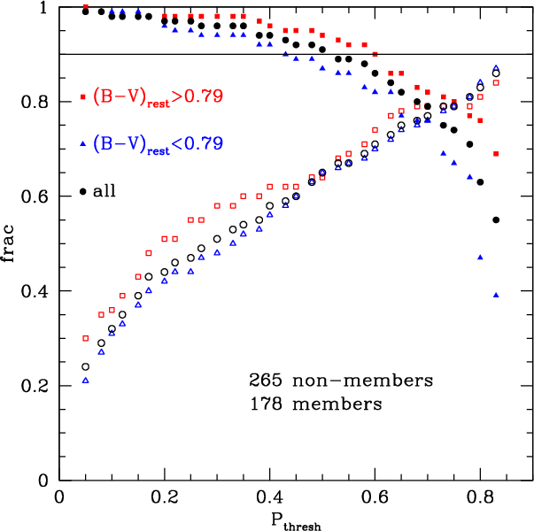
|
Figure 11:
The fraction of retained members and rejected non-members as
a function of the
|
| Open with DEXTER | |
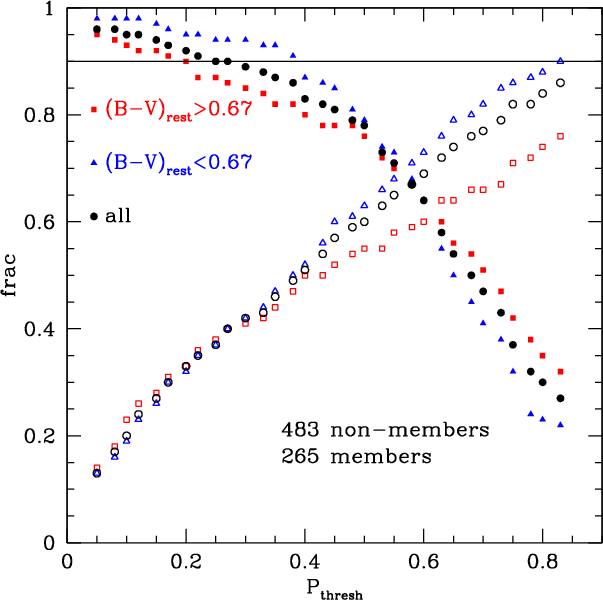
|
Figure 12: Same as Fig. 11 but for clusters with VRIJK photometry. |
| Open with DEXTER | |
Since the performance is similar using Hyperz, we use both codes
jointly to provide the most efficient rejection. In
Figs. 18 and 19, we plot
![]() versus
versus
![]() .
While
there is a large scatter, there is a definite correlation between the
two probabilities, such that the majority of objects with low
.
While
there is a large scatter, there is a definite correlation between the
two probabilities, such that the majority of objects with low
![]() for one code also have a low
for one code also have a low
![]() with the other code. A Spearman's
Rank Correlation test on the distribution of
with the other code. A Spearman's
Rank Correlation test on the distribution of
![]() vs.
vs.
![]() shows that there is higher than
99.9% probability that these two variables are correlated. The same
result is found for the low and high-z samples, when using the full
magnitude-limited samples or other subsamples restricted to the
brightest galaxies. This implies that a joint rejection is feasible.
After extensive tests, we decided to reject galaxies if
shows that there is higher than
99.9% probability that these two variables are correlated. The same
result is found for the low and high-z samples, when using the full
magnitude-limited samples or other subsamples restricted to the
brightest galaxies. This implies that a joint rejection is feasible.
After extensive tests, we decided to reject galaxies if
![]() <
<
![]() for either code; in these tests, the
for either code; in these tests, the
![]() values for each code were determined separately, such that the highest
rejection, independent of rest-frame color, was possible, while
retaining >90% of the confirmed members. The adopted thresholds
are summarized in Table 6 and the performance of
these thresholds is summarized in Table 7.
values for each code were determined separately, such that the highest
rejection, independent of rest-frame color, was possible, while
retaining >90% of the confirmed members. The adopted thresholds
are summarized in Table 6 and the performance of
these thresholds is summarized in Table 7.
Table 6: Rejection thresholds.
Table 7: Retained and rejected fraction in spectroscopic sample
Because P(z) is broader for galaxies without NIR data,
![]() is also
systematically lower and the
is also
systematically lower and the
![]() ,
determined for galaxies with
NIR data, is no longer be applicable. To calibrate
,
determined for galaxies with
NIR data, is no longer be applicable. To calibrate
![]() for
galaxies without NIR data, we re-derived
for
galaxies without NIR data, we re-derived
![]() for the entire
spectroscopic sample, excluding the NIR filters. We recalibrate
for the entire
spectroscopic sample, excluding the NIR filters. We recalibrate
![]() and summarize the performance and adopted cuts in
Tables 6 and 7. It is important to
note that the performance of the rejection is different in areas with
and without NIR data and the retained member population differs in the
two regions. For this reason, we limit all studies using the
photometric redshifts to those areas with NIR data.
and summarize the performance and adopted cuts in
Tables 6 and 7. It is important to
note that the performance of the rejection is different in areas with
and without NIR data and the retained member population differs in the
two regions. For this reason, we limit all studies using the
photometric redshifts to those areas with NIR data.
We checked how the effectiveness of the adopted
![]() varied across
the sample. Because of the limited numbers of spectroscopically
observed objects per cluster, this was not possible on a
cluster-by-cluster basis. Instead we split each of the high-z and
low-z samples into two subsamples each and examined how the accepted
and rejected fractions differed. The retained fractions of members
ranges from 87-98% and the rejected fractions of non-members ranges
from 50-60%.
varied across
the sample. Because of the limited numbers of spectroscopically
observed objects per cluster, this was not possible on a
cluster-by-cluster basis. Instead we split each of the high-z and
low-z samples into two subsamples each and examined how the accepted
and rejected fractions differed. The retained fractions of members
ranges from 87-98% and the rejected fractions of non-members ranges
from 50-60%.
6.3 P clust threshold performance in magnitude limited samples
We examine how applicable our adopted
![]() ,
calibrated using the
spectroscopic subsample, is to the full magnitude-limited sample. In
Fig. 13, we show the apparent magnitude distribution of the
spectroscopic sample and the total photometric sample with the same
magnitude limit, for two clusters in each redshift range with the
widest spectroscopic coverage. It is clear from these plots that we
are not spectroscopically complete at any magnitude and that the
spectroscopic sample, as expected, is biased towards brighter
magnitudes.
,
calibrated using the
spectroscopic subsample, is to the full magnitude-limited sample. In
Fig. 13, we show the apparent magnitude distribution of the
spectroscopic sample and the total photometric sample with the same
magnitude limit, for two clusters in each redshift range with the
widest spectroscopic coverage. It is clear from these plots that we
are not spectroscopically complete at any magnitude and that the
spectroscopic sample, as expected, is biased towards brighter
magnitudes.
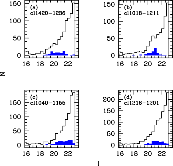
|
Figure 13: The apparent magnitude histograms for the spectroscopic sample (solid blue histogram) versus the total sample of the same limiting magnitude (open black). For both samples at low-z (a and b) and high-z (c and d), two of the clusters with the most complete spectroscopic coverage are displayed. We note that the spectroscopic sample, even for clusters with the most extensive spectroscopy, is not complete at any magnitude limit and is biased towards brighter magnitudes. The magnitudes correspond to the I-band AUTO magnitudes from SExtractor. |
| Open with DEXTER | |
The spectroscopic target lists were not only constructed with a
magnitude limit in mind, but also with an eye towards reducing the
number of galaxies that had low probabilities of being at the cluster
redshift, in addition to including some galaxies that were not
formally present about
![]() .
We examine in general how this
preselection causes the
.
We examine in general how this
preselection causes the
![]() distributions of the spectroscopic
sample to differ from those in a magnitude-limited photometric
sample. In Fig. 20, we compare the histogram of the
distributions of the spectroscopic
sample to differ from those in a magnitude-limited photometric
sample. In Fig. 20, we compare the histogram of the
![]() values for the spectroscopic samples with those for the entire
sample down to the same magnitude limits. The spectroscopic
preselection manifests itself as an excess of high
values for the spectroscopic samples with those for the entire
sample down to the same magnitude limits. The spectroscopic
preselection manifests itself as an excess of high
![]() values and
a deficit of low
values and
a deficit of low
![]() for the spectroscopic sample with respect to
the photometric sample.
Within the precision of our numerical routine, a KS-test gives 0%
probability that these two distributions are drawn from the same parent
distribution.
This inherent bias implies that a certain
for the spectroscopic sample with respect to
the photometric sample.
Within the precision of our numerical routine, a KS-test gives 0%
probability that these two distributions are drawn from the same parent
distribution.
This inherent bias implies that a certain
![]() removes a higher fraction of galaxies in the photometric
sample than was the case in the spectroscopic subsample.
removes a higher fraction of galaxies in the photometric
sample than was the case in the spectroscopic subsample.
We examine how the spectroscopically calibrated
![]() rejection
operates when applied to a magnitude-limited sample. We illustrate these
results using the GR code, but the conclusions would be equivalent using
Hyperz. In Figs. 14,
21, 15, and
22, we plot the
rejection
operates when applied to a magnitude-limited sample. We illustrate these
results using the GR code, but the conclusions would be equivalent using
Hyperz. In Figs. 14,
21, 15, and
22, we plot the
![]() versus
versus
![]() for two high-zand two low-z clusters. Each figure has panels that show how this
distribution changes with apparent magnitude. As we move to fainter
magnitude limits, many galaxies appear at all
for two high-zand two low-z clusters. Each figure has panels that show how this
distribution changes with apparent magnitude. As we move to fainter
magnitude limits, many galaxies appear at all
![]() values. Those at
high
values. Those at
high
![]() do indeed fall close to
do indeed fall close to
![]() ,
as predicted by the
spectroscopic studies. Encouragingly, the galaxies with low
,
as predicted by the
spectroscopic studies. Encouragingly, the galaxies with low
![]() values fall systematically away from
values fall systematically away from
![]() .
In fact, even at the
faintest magnitudes, there are very few galaxies within
.
In fact, even at the
faintest magnitudes, there are very few galaxies within
![]()
![]() 0.1 that have
0.1 that have
![]() < 0.2. We recall that this must not
be the case: galaxies with
< 0.2. We recall that this must not
be the case: galaxies with
![]()
![]()
![]() but broad P(z)
distributions will have low probabilities of being at the cluster
redshift, even though their best value lies around
but broad P(z)
distributions will have low probabilities of being at the cluster
redshift, even though their best value lies around
![]() .
This
self-consistency implies that
.
This
self-consistency implies that
![]() is, in fact, providing us with a
real indication of whether these faint objects are at the cluster
redshift. This effect would be difficult to reproduce by systematic
errors in the photometric redshifts because it appears for all
clusters, regardless of their redshift range or presence of NIR data.
Nonetheless, there are some faint galaxies with
is, in fact, providing us with a
real indication of whether these faint objects are at the cluster
redshift. This effect would be difficult to reproduce by systematic
errors in the photometric redshifts because it appears for all
clusters, regardless of their redshift range or presence of NIR data.
Nonetheless, there are some faint galaxies with
![]() that may be rejected because of a broad P(z). Also, the
tests presented in Sect. 4.3 demonstrate that the
photometric redshift accuracy is expected to be lower for fainter
galaxies, implying that there will be galaxies who are truly at
that may be rejected because of a broad P(z). Also, the
tests presented in Sect. 4.3 demonstrate that the
photometric redshift accuracy is expected to be lower for fainter
galaxies, implying that there will be galaxies who are truly at
![]() but are scattered away from the cluster redshift. In
Rudnick et al. (2009), we discuss how these effects may differ
for red and blue galaxies and we present the implications for the
study of the cluster galaxy luminosity function.
but are scattered away from the cluster redshift. In
Rudnick et al. (2009), we discuss how these effects may differ
for red and blue galaxies and we present the implications for the
study of the cluster galaxy luminosity function.
The total fraction of galaxies rejected for each cluster as a function of I magnitude are presented in the Cols. 3-6 of Table 8. When our rejection criteria is applied, we reject 55-82% of the galaxies at I<22 and 75-93% at I<24.5.
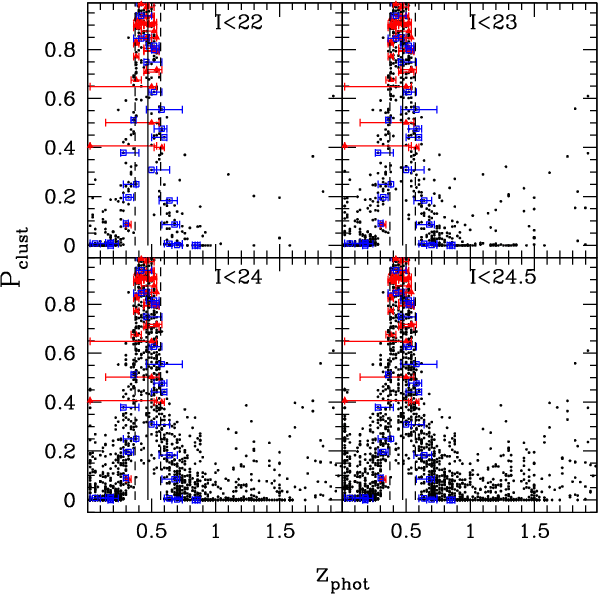
|
Figure 14:
A plot of
|
| Open with DEXTER | |
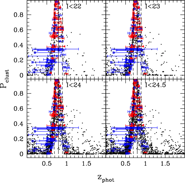
|
Figure 15: Same as Fig. 14 except for Cl1216-1201. |
| Open with DEXTER | |
Table 8:
Total fraction of galaxies rejected as cluster members as a function of
the I magnitude (Cols. 3 to 6 for ![]() ,
23, 24 and 24.5 respectively).
,
23, 24 and 24.5 respectively).
7 Discussion and conclusions
We have used two independent codes to compute photometric redshifts:
Hyperz and GR code. In general, the two codes yield rather
similar results, either on a cluster-by-cluster basis or as a function
of the filter set and spectral type, of typically
![]() to 0.06. Hyperz results are found to be
slightly more accurate than GR's ones in general, by
to 0.06. Hyperz results are found to be
slightly more accurate than GR's ones in general, by ![]() 20%
in
20%
in
![]() .
The quality achieved by both codes is
consistent with the expectations derived from ``ideal'' simulations.
An interesting trend is that the quality of both codes is highly
correlated, in the sense that the highest and lowest quality results,
in terms of
.
The quality achieved by both codes is
consistent with the expectations derived from ``ideal'' simulations.
An interesting trend is that the quality of both codes is highly
correlated, in the sense that the highest and lowest quality results,
in terms of
![]() ,
and systematics are found for
the same clusters. This trend cannot be due to the use of an
incomplete or imperfect template set, as suggested by other authors
(Ilbert et al. 2006), because in such a case, we should expect the
same systematic behavior in all fields, given a filter set, as
discussed in Sect. 4.1. In contrast, different systematics are
observed in the different fields, which are found to be almost equal
for the two independent
,
and systematics are found for
the same clusters. This trend cannot be due to the use of an
incomplete or imperfect template set, as suggested by other authors
(Ilbert et al. 2006), because in such a case, we should expect the
same systematic behavior in all fields, given a filter set, as
discussed in Sect. 4.1. In contrast, different systematics are
observed in the different fields, which are found to be almost equal
for the two independent
![]() codes. This behavior suggests that the
origin of the systematic errors is more likely to be associated with
small residuals in the input photometry rather than the
codes. This behavior suggests that the
origin of the systematic errors is more likely to be associated with
small residuals in the input photometry rather than the
![]() templates and codes. Indeed, small zero-point shifts of
templates and codes. Indeed, small zero-point shifts of
![]() 0.05 mag cannot be excluded, in particular for the
near-IR data.
0.05 mag cannot be excluded, in particular for the
near-IR data.
Photometric redshifts are found to be particularly useful in the
identification and study of galaxy clusters in large surveys. The
determination of cluster redshifts in the EDisCS fields using a simple
algorithm based on
![]() is highly accurate. Indeed, the differences
between photometric and spectroscopic values are found to be small,
typically ranging between
is highly accurate. Indeed, the differences
between photometric and spectroscopic values are found to be small,
typically ranging between
![]() 0.03-0.04 in the high-zsample and
0.03-0.04 in the high-zsample and
![]() in the low-z sample. This is at least a
factor
in the low-z sample. This is at least a
factor ![]() more accurate than the determination of
more accurate than the determination of
![]() for
individual galaxies. The accuracy is more sensitive to the filter set
used rather than the redshift of the cluster. The systematic lower
quality results for the low-z sample was somewhat expected from the
simulations presented in Sect. 4.1.
Tomography based on
for
individual galaxies. The accuracy is more sensitive to the filter set
used rather than the redshift of the cluster. The systematic lower
quality results for the low-z sample was somewhat expected from the
simulations presented in Sect. 4.1.
Tomography based on
![]() could be used in searches for clusters
along the line-of-sight, using redshift steps optimized to be close in
value to the typical difference between photometric and spectroscopic
could be used in searches for clusters
along the line-of-sight, using redshift steps optimized to be close in
value to the typical difference between photometric and spectroscopic
![]() to maximize the contrast between members and non-member
galaxies (in this case,
to maximize the contrast between members and non-member
galaxies (in this case,
![]() ).
).
The cluster membership criterion presented in Sect. 6 has been used to extend the spectroscopic studies of cluster galaxies to fainter limits in magnitude (e.g. De Lucia et al. 2004; White et al. 2005; Clowe et al. 2006; Poggianti et al. 2006; De Lucia et al. 2007; Desai et al. 2007; Rudnick et al. 2009).
In conclusion, photometric redshifts are useful tools for studying galaxy clusters. They enable efficient and complete pre-selection of cluster members for spectroscopy, allow accurate determinations of the cluster redshifts based on photometry alone, provide a means of determining cluster membership, especially for bright sources, and can be used to search for galaxy clusters.
AcknowledgementsPart of this work was supported by the French Centre National de la Recherche Scientifique, by the French Programme National de Cosmologie (PNC) and the Programme National Galaxies (PNG). The Dark Cosmology Centre is funded by the Danish National Research Foundation.
References
- Avni, Y. 1976, ApJ, 210, 642 [NASA ADS] [CrossRef]
- Banerji, M., Abdalla, F. B., Lahav, O., & Lin, H. 2008, MNRAS, 386, 1219 [NASA ADS] [CrossRef]
- Bertin, E., & Arnouts, S. 1996, A&ASS, 117, 393 [NASA ADS] [CrossRef]
- Bolzonella, M., Miralles, J. M., & Pelló, R. 2000, A&A, 363, 476 [NASA ADS]
- Brunner, R. J., & Lubin, L. M. 2000, AJ, 120, 2851 [NASA ADS] [CrossRef]
- Bruzual, G., & Charlot, S. 1993, ApJ 405, 538
- Bruzual, G., & Charlot, S. 2003, MNRAS, 344, 1000 [NASA ADS] [CrossRef]
- Chabrier, G. 2003, PASP, 115, 763 [NASA ADS] [CrossRef]
- Calzetti, D., Armus, L., Bohlin, R. C., et al. 2000, ApJ, 533, 682 [NASA ADS] [CrossRef]
- Capak, P., Aussel, H., Ajiki, M., et al. 2007, ApJS, 172, 99 [NASA ADS] [CrossRef]
- Coe, D., Benítez, N., Sánchez, S. F., et al. 2006, AJ, 132, 926 [NASA ADS] [CrossRef]
- Coleman, D. G., Wu, C. C., & Weedman, D. W. 1980, ApJS, 43, 393 [NASA ADS] [CrossRef]
- Clowe, D., Schneider, P., Aragón-Salamanca, A., et al. 2006, A&A, 451, 395 [NASA ADS] [EDP Sciences] [CrossRef]
- De Lucia, G., Poggianti, B. M., Aragón-Salamanca, A., et al. 2004, ApJ, 610, L77 [NASA ADS] [CrossRef]
- De Lucia, G., Poggianti, B. M., Aragón-Salamanca, A., et al. 2007, MNRAS, 374, 809 [NASA ADS] [CrossRef]
- Dressler, A. 1980, ApJ, 236, 351 [NASA ADS] [CrossRef]
- Desai, V., Dalcanton, J. J., Aragón-Salamanca, A., et al. 2007, ApJ, 660, 1151 [NASA ADS] [CrossRef]
- Feldmann, R., Carollo, C. M., Porciani, C., et al. 2006, MNRAS, 372, 565 [NASA ADS] [CrossRef]
- Finn, R. A., Zaritsky D., McCarthy, D. W. Jr, et al. 2005, ApJ, 630, 206 [NASA ADS] [CrossRef]
- Gonzalez, A. H., Zaritsky, D., Dalcanton, J. J., & Nelson, A. 2001, ApJS, 137, 117 [NASA ADS] [CrossRef]
- Halliday, C., Milvang-Jensen, B., Poirier, S., et al. 2004, A&A, 427, 397 [NASA ADS] [EDP Sciences] [CrossRef]
- Hatziminaoglou, E., Mathez, G., & Pelló, R. 2000, A&A, 359, 9 [NASA ADS]
- Hildebrandt, H., Wolf, C., & Benítez, N. 2008, A&A, 480, 703 [NASA ADS] [EDP Sciences] [CrossRef]
- Ilbert, O., Arnouts, S., McCracken, H. J., et al. 2006, A&A, 457, 841 [NASA ADS] [EDP Sciences] [CrossRef]
- Ilbert, O., Capak, P., Salvato, M., et al. 2009, ApJ, 690, 1236 [NASA ADS] [CrossRef]
- Johnson, O., Best, P., Zaritsky, D., et al. 2006, MNRAS, 371, 1777 [NASA ADS] [CrossRef]
- Kinney, A. L., Calzetti, D., Bohlin, R. C., et al. 1996, ApJ, 467, 38 [NASA ADS] [CrossRef]
- Li, I. H., & Yee, H. K. C. 2008, AJ, 135, 809 [NASA ADS] [CrossRef]
- Margoniner, V. E., & Wittman, D. M. 2008, ApJ, 679, 31 [NASA ADS] [CrossRef]
- Miller, G. E., & Scalo, J. M. 1979, ApJS, 41, 513 [NASA ADS] [CrossRef]
- Milvang-Jensen, B., Noll, S., Halliday, C., et al. 2008, A&A, 482, 419 [NASA ADS] [EDP Sciences] [CrossRef]
- Mobasher, B., Capak, P., Scoville, N. Z., et al. 2007, ApJS, 172, 117 [NASA ADS] [CrossRef]
- Pickles, A. J. 1998, PASP, 110, 863 [NASA ADS] [CrossRef]
- Poggianti, B. M., von der Linden, A., De Lucia, G., et al. 2006, ApJ, 642, 188 [NASA ADS] [CrossRef]
- Rudnick, G., Franx, M., Rix, H.-W., et al. 2001, AJ, 122, 2205 [NASA ADS] [CrossRef]
- Rudnick, G. M., Rix, H.- W., Franx, M., et al. 2003, ApJ, 599, 847 [NASA ADS] [CrossRef]
- Rudnick, G. M., von der Linden, A., Pelló, R., et al. 2009, ApJ, 700, 1559 [NASA ADS] [CrossRef]
- Salpeter, E. E. 1955, ApJ, 121, 161 [NASA ADS] [CrossRef]
- Schlegel, D. J., Finkbeiner, D. P., & Davis, M. 1998, ApJ, 500, 525 [NASA ADS] [CrossRef]
- Toft, S., Mainieri, V., Rosati, P., et al. 2004, A&A, 422, 29 [NASA ADS] [EDP Sciences] [CrossRef]
- Whiley, I. M., Aragón-Salamanca, A., De Lucia, G., et al. 2008, MNRAS, 387, 1253 [NASA ADS] [CrossRef]
- White, S. D. M., Clowe, D. I., Simard, L., et al. 2005, A&A, 444, 365 [NASA ADS] [EDP Sciences] [CrossRef]
Online Material
Table 9:
![]() accuracy derived from simulations for
galaxies in the spectroscopic sample, based on the GR code.
accuracy derived from simulations for
galaxies in the spectroscopic sample, based on the GR code.
Table 10:
![]() accuracy expected for the faintest galaxies in the
EDisCS sample, based on the GR code.
accuracy expected for the faintest galaxies in the
EDisCS sample, based on the GR code.
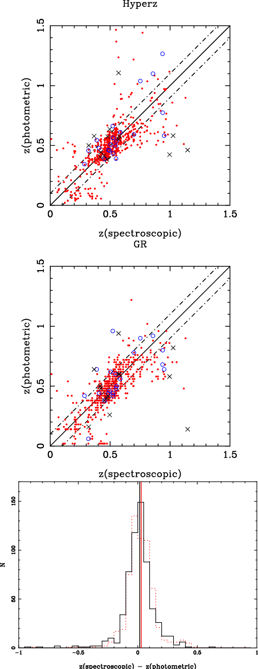
|
Figure 16:
Comparison between spectroscopic and photometric redshifts
for the low-z sample, obtained with Hyperz ( top panel) and
GR ( central panel)
codes. Solid (red) circles, open (blue) circles, and crosses correspond
to objects with good (type 1), medium (type 2) and tentative
(type 3) spectroscopic redshift determinations, respectively.
Dot-dashed lines display
|
| Open with DEXTER | |
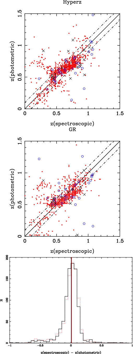
|
Figure 17:
(Comparison between spectroscopic and photometric redshifts
for the high-z sample, obtained with Hyperz ( top panel) and
GR ( central panel)
codes. Solid (red) circles, open (blue) circles, and crosses correspond
to objects with good (type 1), medium (type 2) and tentative
(type 3) spectroscopic redshift determinations, respectively.
Dot-dashed lines display
|
| Open with DEXTER | |
|
Figure 18:
A comparison of
|
| Open with DEXTER | |
|
Figure 19: Same as Fig. 18 but for the clusters with VRIJK photometry. |
| Open with DEXTER | |
|
Figure 20:
The histogram of
|
| Open with DEXTER | |
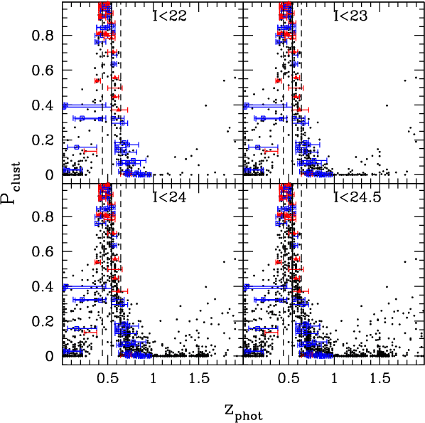
|
Figure 21: Same as Fig. 14 except for Cl1420-1236. |
| Open with DEXTER | |
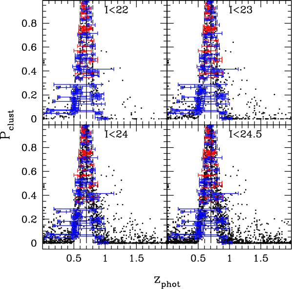
|
Figure 22: Same as Fig. 14 except for Cl1040-1155. |
| Open with DEXTER | |
Footnotes
- ... Survey
- Based on observations collected at the European Southern Observatory, Paranal and La Silla, Chile, as part of the ESO LP 166.A-0162.
- ...
- Figures 16-22, Tables 9 and 10 are only available in electronic form at http://www.aanda.org
- ...
website
- http://www.mpa-garching.mpg.de/galform/ediscs
- ...
website
- http://www.mpa-garching.mpg.de/galform/ediscs
- ... Hyperz
- http://webast.ast.obs-mip.fr/hyperz/
- ...
website
- http://www.mpa-garching.mpg.de/galform/ediscs
All Tables
Table 1:
![]() accuracy from simulations
for galaxies in the spectroscopic sample, based on Hyperz.
accuracy from simulations
for galaxies in the spectroscopic sample, based on Hyperz.
Table 2:
![]() accuracy expected for the faintest galaxies in the
EDisCS sample, in the low-z and high-z fields, based on Hyperz.
accuracy expected for the faintest galaxies in the
EDisCS sample, in the low-z and high-z fields, based on Hyperz.
Table 3:
Summary of
![]() accuracy achieved for the
individual low-z and high-z clusters.
accuracy achieved for the
individual low-z and high-z clusters.
Table 4:
Summary of
![]() accuracy achieved for the
whole low-z and high-z samples with Hyperz and GR codes.
accuracy achieved for the
whole low-z and high-z samples with Hyperz and GR codes.
Table 5:
Comparison between spectroscopic (
![]() )
and photometric
determinations of cluster redshifts in the low and high-z samples.
)
and photometric
determinations of cluster redshifts in the low and high-z samples.
Table 6: Rejection thresholds.
Table 7: Retained and rejected fraction in spectroscopic sample
Table 8:
Total fraction of galaxies rejected as cluster members as a function of
the I magnitude (Cols. 3 to 6 for ![]() ,
23, 24 and 24.5 respectively).
,
23, 24 and 24.5 respectively).
Table 9:
![]() accuracy derived from simulations for
galaxies in the spectroscopic sample, based on the GR code.
accuracy derived from simulations for
galaxies in the spectroscopic sample, based on the GR code.
Table 10:
![]() accuracy expected for the faintest galaxies in the
EDisCS sample, based on the GR code.
accuracy expected for the faintest galaxies in the
EDisCS sample, based on the GR code.
All Figures
|
|
Figure 1:
Photometric versus model redshifts retrieved from
|
| Open with DEXTER | |
| In the text | |
|
|
Figure 2:
Photometric versus model redshifts retrieved from
|
| Open with DEXTER | |
| In the text | |
|
|
Figure 3:
These figures present the expected
|
| Open with DEXTER | |
| In the text | |
|
|
Figure 4:
(
|
| Open with DEXTER | |
| In the text | |
|
|
Figure 5:
(
|
| Open with DEXTER | |
| In the text | |
|
|
Figure 6:
Photometric redshift distributions in the EDisCS fields,
with the cluster redshift increasing from top to bottom and from
left to right,
for the low-z and high-z samples (first and second series respectively).
The histograms display the following redshift
distributions:
|
| Open with DEXTER | |
| In the text | |
|
|
Figure 7:
Projected number density maps for the low-z sample, for
different redshift slices with
|
| Open with DEXTER | |
| In the text | |
|
|
Figure 8: Projected number density maps for the high-z sample, for different redshift slices. Same comments as in Fig. 7. There is no clear BCG identified in Cl1122-1136. |
| Open with DEXTER | |
| In the text | |
|
|
Figure 9:
The integrated probability of being at
|
| Open with DEXTER | |
| In the text | |
|
|
Figure 10: Same as Fig. 9 but for the high-z clusters. |
| Open with DEXTER | |
| In the text | |
|
|
Figure 11:
The fraction of retained members and rejected non-members as
a function of the
|
| Open with DEXTER | |
| In the text | |
|
|
Figure 12: Same as Fig. 11 but for clusters with VRIJK photometry. |
| Open with DEXTER | |
| In the text | |
|
|
Figure 13: The apparent magnitude histograms for the spectroscopic sample (solid blue histogram) versus the total sample of the same limiting magnitude (open black). For both samples at low-z (a and b) and high-z (c and d), two of the clusters with the most complete spectroscopic coverage are displayed. We note that the spectroscopic sample, even for clusters with the most extensive spectroscopy, is not complete at any magnitude limit and is biased towards brighter magnitudes. The magnitudes correspond to the I-band AUTO magnitudes from SExtractor. |
| Open with DEXTER | |
| In the text | |
|
|
Figure 14:
A plot of
|
| Open with DEXTER | |
| In the text | |
|
|
Figure 15: Same as Fig. 14 except for Cl1216-1201. |
| Open with DEXTER | |
| In the text | |
|
|
Figure 16:
Comparison between spectroscopic and photometric redshifts
for the low-z sample, obtained with Hyperz ( top panel) and
GR ( central panel)
codes. Solid (red) circles, open (blue) circles, and crosses correspond
to objects with good (type 1), medium (type 2) and tentative
(type 3) spectroscopic redshift determinations, respectively.
Dot-dashed lines display
|
| Open with DEXTER | |
| In the text | |
|
|
Figure 17:
(Comparison between spectroscopic and photometric redshifts
for the high-z sample, obtained with Hyperz ( top panel) and
GR ( central panel)
codes. Solid (red) circles, open (blue) circles, and crosses correspond
to objects with good (type 1), medium (type 2) and tentative
(type 3) spectroscopic redshift determinations, respectively.
Dot-dashed lines display
|
| Open with DEXTER | |
| In the text | |
|
|
Figure 18:
A comparison of
|
| Open with DEXTER | |
| In the text | |
|
|
Figure 19: Same as Fig. 18 but for the clusters with VRIJK photometry. |
| Open with DEXTER | |
| In the text | |
|
|
Figure 20:
The histogram of
|
| Open with DEXTER | |
| In the text | |
|
|
Figure 21: Same as Fig. 14 except for Cl1420-1236. |
| Open with DEXTER | |
| In the text | |
|
|
Figure 22: Same as Fig. 14 except for Cl1040-1155. |
| Open with DEXTER | |
| In the text | |
Copyright ESO 2009
Current usage metrics show cumulative count of Article Views (full-text article views including HTML views, PDF and ePub downloads, according to the available data) and Abstracts Views on Vision4Press platform.
Data correspond to usage on the plateform after 2015. The current usage metrics is available 48-96 hours after online publication and is updated daily on week days.
Initial download of the metrics may take a while.