| Issue |
A&A
Volume 506, Number 2, November I 2009
|
|
|---|---|---|
| Page(s) | 647 - 660 | |
| Section | Cosmology (including clusters of galaxies) | |
| DOI | https://doi.org/10.1051/0004-6361/200911787 | |
| Published online | 27 August 2009 | |
A&A 506, 647-660 (2009)
Building merger trees from cosmological N-body simulations
Towards improving galaxy formation models
using subhaloes![[*]](/icons/foot_motif.png)
D. Tweed1,2 - J. Devriendt1,2 - J. Blaizot1 - S. Colombi3 - A. Slyz2
1 - Université de Lyon, 69003 Lyon; Université Lyon 1,
Villeurbanne; CNRS, UMR 5574, Centre de Recherche Astrophysique de
Lyon; Observatoire de Lyon, 69230 Saint-Genis Laval; École Normale
Supérieure de Lyon, 69007 Lyon, France
2 - Astrophysics, University of Oxford, Keble Road, Oxford OX1 3RH, UK
3 - Institut Astrophysique de Paris (IAP), 98bis boulevard Arago, 75014
Paris, France
Received 4 February 2009 / Accepted 3 August 2009
Abstract
Context. In the past decade or so, using numerical N-body
simulations to describe the gravitational clustering of dark matter
(DM) in an expanding universe has become the tool of choice for
tackling the issue of hierarchical galaxy formation. As mass resolution
increases with the power of supercomputers, one is able to grasp finer
and finer details of this process, resolving more and more of the inner
structure of collapsed objects. This begs one to revisit time and again
the post-processing tools with which one transforms particles into
``invisible'' dark matter haloes and from thereon into luminous
galaxies.
Aims. Although a fair amount of work has been
devoted to growing Monte-Carlo merger trees that resemble those built
from an N-body simulation, comparatively little
effort has been invested in quantifying the caveats one necessarily
encounters when one extracts trees directly from such a simulation. To
somewhat revert the tide, this paper seeks to provide its reader with a
comprehensive study of the problems one faces when following this
route.
Methods. The first step in building merger histories
of dark matter haloes and their subhaloes is to identify these
structures in each of the time outputs (snapshots) produced by the
simulation. Even though we discuss a particular implementation of such
an algorithm (called AdaptaHOP) in this paper, we believe that our
results do not depend on the exact details of the implementation but
instead extend to most if not all (sub)structure finders. To illustrate
this point in the appendix we compare AdaptaHOP's results to the
standard friend-of-friend (FOF) algorithm, widely utilised in the
astrophysical community. We then highlight different ways of building
merger histories from AdaptaHOP haloes and subhaloes, contrasting their
various advantages and drawbacks.
Results. We find that the best approach to (sub)halo
merging histories is through an analysis that goes back and forth
between identification and tree building rather than one that conducts
a straightforward sequential treatment of these two steps. This is
rooted in the complexity of the merging trees that have to depict an
inherently dynamical process from the partial temporal information
contained in the collection of instantaneous snapshots available from
the N-body simulation. However, we also propose a
simpler sequential ``Most massive Substructure Method'' (MSM) whose
trees approximate those obtained via the more complicated non
sequential method.
Key words: methods: numerical - methods: N-body simulations - cosmology: large-scale structure of Universe
1 Introduction
Dark matter haloes and their mass assembly histories are the
fundamental bricks of any nonlinear structure formation theory based on
the current concordance (![]() CDM)
model that has been so successful at reproducing large scale structure
data
(Dunkley et al. 2009).
It is therefore natural that a lot of effort has been devoted to
finding semi-analytic descriptions of this process.
These culminated with the seminal papers on the extended Press
Schechter (EPS) formalism (Lacey & Cole 1994; Bond
et al. 1991), as it became possible to make
Monte-Carlo realisations of merging histories of haloes using EPS.
However, it was also realised early on that shortcomings of the EPS
theory needed to be circumvented (non spherical collapse, loss of
internal structure, no spatial information) to get accurate halo mass
distributions
and merging tree histories (Sheth & Lemson 1999;
Somerville
& Primack 1999).
CDM)
model that has been so successful at reproducing large scale structure
data
(Dunkley et al. 2009).
It is therefore natural that a lot of effort has been devoted to
finding semi-analytic descriptions of this process.
These culminated with the seminal papers on the extended Press
Schechter (EPS) formalism (Lacey & Cole 1994; Bond
et al. 1991), as it became possible to make
Monte-Carlo realisations of merging histories of haloes using EPS.
However, it was also realised early on that shortcomings of the EPS
theory needed to be circumvented (non spherical collapse, loss of
internal structure, no spatial information) to get accurate halo mass
distributions
and merging tree histories (Sheth & Lemson 1999;
Somerville
& Primack 1999).
For a detailed critique of the EPS theory, we refer the interested reader to Benson et al. (2005), however we point out one of the most worrisome of its shortcomings. It may seem legitimate to generate merging trees for a representative sample of haloes at a given redshift and then attempt to construct the halo mass function at an earlier time, combining the branches of these Monte-Carlo merging trees, with each branch appropriately weighted according to the EPS theory. However, in doing so, one will not obtain good agreement between this mass function and the mass function of haloes extracted directly from N-body simulations at this early epoch. This discrepancy can be tuned empirically, but there is no theoretical justification as to why such a correction should be made (Benson et al. 2001). This explains why people calibrate Monte-Carlo merging trees against those generated using N-body simulations, as done recently by Neistein & Dekel (2008) and Parkinson et al. (2008). Indeed merging trees directly built from N-body simulations naturally circumvent the shortcomings of the Monte-Carlo methods. Moreover with the democratisation of (super)computer power N-body simulations are becoming more and more available and resolved, and this implies that it will inevitably make more and more sense to build trees directly from them in the future.
However, as underlined in the hierarchical galaxy formation primer of Baugh (2006), the construction of a merger tree from the outputs of an N-body simulation is not a trivial matter. The mass of a halo can decrease with time since haloes may spatially overlap one another at a given time output and therefore be blended together by the group-finding algorithm, then separate at the next time output for good, or come back together again later on. This paper is therefore devoted to identifying and quantifying the occurrences of these ``anomalies'' that plague N-body merger trees. It also proposes different methods of dealing with them and contrasts/compares their advantages and disadvantages.
Its outline is as follows: in the first part (Sect. 2) we discuss the issue of dark matter halo and subhalo detection in cosmological N-body simulations; in the second (Sect. 3) we build N-body merger histories based on three methods we use to construct subhaloes. We use these merger trees to pitch these methods against one another. We draw our conclusions in the third part (Sect. 4).
2 Dark matter halo and subhalo detection
Most algorithms commonly used to identify dark matter haloes in N-body cosmological simulations are based either on a percolation algorithm, as the so called friend-of-friend (FOF) algorithm (Huchra & Geller 1982; Davis et al. 1985) or a prescription to identify local maxima of the density field (e.g. DENMAX, Gelb & Bertschinger 1994; SOD, Lacey & Cole 1994; BDM, Klypin et al. 1999; HOP, Eisenstein & Hut 1998). With computational power rapidly increasing, these algorithms have been recently extended to probe the inner structure of the haloes and detect subhaloes within them (e.g. IsoDen, Pfitzner & Salmon 1996; SKID, Ghigna et al. 1998; HFOF, Klypin et al. 1999; SUBFIND, Springel et al. 2001; AdaptaHOP, Aubert et al. 2004; MHF, Gill et al. 2004; and its successor AHF, Knollmann & Knebe 2009).
Note however that, in the best of cases, these algorithms proceed in two consecutive steps: first they identify the halo in real (3 dimensional (3D)) space, and then they use velocity space information to ``refine'' the composition of their haloes (i.e. decide if a particle is gravitationally bound to it or not). Ultimately, to obtain the most reliable results, one would want to define haloes as structures detected directly in the 6 dimensional (6D) phase space (for a review and extensive comparison of the methods which have been proposed to do that see Maciejewski et al. 2009a), but the developments in that direction are pretty recent (Maciejewski et al. 2009b; Diemand et al. 2006) so our approach in this paper remains three dimensional. Moreover, in practise, the bound structures detected in 6D space are not very different from the 3D ones, except that they tend to be systematically (albeit slightly) more massive (Maciejewski et al. 2009b).
In light of the previous comments, we feel it is a fair claim to say that none of the 3D algorithms are completely satisfactory, and that the results of the analysis of any output of a cosmological N-body simulation in terms of halo/subhalo detection will, to a certain extent, depend on the choice of algorithm used to perform that detection. Bearing these limitations in mind we choose AdaptaHOP (Aubert et al. 2004) as our halo and subhalo finder in this work.
We first start by a brief description of this algorithm. We then discuss the advantages and disadvantages arising from three natural but different methods to select subhaloes with AdaptaHOP: the density profile method (DPM), the Most massive Sub-node Method (MSM) and the branch history method (BHM).
2.1 Dark matter halo detection
In this section, we will be concerned with the way one can split an ensemble of particles in N-body simulation snapshots into DM haloes and subhaloes. In other words, we want to group together particles on the basis of the instantaneous values of their positions (and velocities) alone, using the a priori knowledge gleaned from the N-body simulation itself that positions contain the most accurate information. However, already at this point, we emphasise that the merger history of haloes are imprinted in the particle distribution. For instance, after a merger with another halo, a structure can survive as a subhalo which will be present as a local density maxima within the particle distribution of its host halo.
In the appendix, we compare in details the most widely used
halo finder FOF to the
AdaptaHOP algorithm that we will use to monitor substructure. Here, we
simply point out that FOF consists in grouping together particles which
are closer than a distance ![]() (mean
inter-particle distance). Usually
b is chosen to be 0.2, which closely matches an
average halo over-density of
(mean
inter-particle distance). Usually
b is chosen to be 0.2, which closely matches an
average halo over-density of
![]() (where
(where ![]() is the critical density, i.e. the matter density necessary for the
Universe to
be flat in the absence of other energy sources), obtained when solving
the classic spherical collapse of a ``top-hat''
density perturbation in an Einstein-de Sitter universe. To optimise the
mass resolution of the N-body simulation, haloes
containing at least 20 particles are considered
as bound objects. Obviously, using such a threshold is not the best way
to select
bound structures, because (i) it ignores the kinetic and potential
energy of particles (ii) even if it was energetically justified, a halo
sitting exactly on the threshold could still ``lose'' a particle by
interacting with its environment and not be detected in the following
snapshot of the simulation. However, computing the potential energy of
each particle belonging to a halo is very expensive CPU wise, and at
the same time
inaccurate due to both the pre-selection process of the halo members,
which is necessarily based on a somewhat arbitrary spatial/velocity
density cut, and the necessity to make do with a small number of
particles per halo to maximise the halo mass range spanned by the
simulation.
This experimental threshold of 20 is justified a posteriori by the fact
that provided the time span between snapshots is not much larger than
200 Myr, less than 30% of haloes with this many particles are
lost
between two consecutive outputs (see e.g. Fig. A.4).
is the critical density, i.e. the matter density necessary for the
Universe to
be flat in the absence of other energy sources), obtained when solving
the classic spherical collapse of a ``top-hat''
density perturbation in an Einstein-de Sitter universe. To optimise the
mass resolution of the N-body simulation, haloes
containing at least 20 particles are considered
as bound objects. Obviously, using such a threshold is not the best way
to select
bound structures, because (i) it ignores the kinetic and potential
energy of particles (ii) even if it was energetically justified, a halo
sitting exactly on the threshold could still ``lose'' a particle by
interacting with its environment and not be detected in the following
snapshot of the simulation. However, computing the potential energy of
each particle belonging to a halo is very expensive CPU wise, and at
the same time
inaccurate due to both the pre-selection process of the halo members,
which is necessarily based on a somewhat arbitrary spatial/velocity
density cut, and the necessity to make do with a small number of
particles per halo to maximise the halo mass range spanned by the
simulation.
This experimental threshold of 20 is justified a posteriori by the fact
that provided the time span between snapshots is not much larger than
200 Myr, less than 30% of haloes with this many particles are
lost
between two consecutive outputs (see e.g. Fig. A.4).
In principle, the simple FOF algorithm can be used to detect substructures, simply by running with smaller and smaller values for the linking length (Klypin et al. 1999). However, this method is quite inefficient because a whole range of values for b needs to be explored since real substructures (i) are embedded within one another and (ii) have different density contrasts due to a different epoch of collapse and tidal encounters. Furthermore, there exists no obvious physical criterion to pick the ``best'' value of b corresponding to a global level of substructure, as such a criterion would depend on merging history and therefore is prone to vary from object to object.
Instead of relying directly on single particle positions to identify substructure as the FOF would do, we can go a small step further and remark that substructures are going to be located at local maxima of their host halo density field, so that the natural way to detect them is to compute this density field. This simple assertion constitutes the core of the AdaptaHOP algorithm (as well as that of many others that we listed earlier) which can roughly be summarised by the following steps (see Appendix B of Aubert et al. 2004, for details):
- 1.
- For each particle in the N-body
simulation, find the n closest neighbours using
your favourite oct-tree algorithm (n has a typical
value comprised between 20 and 64, we use 20 in this paper). The
density
 ,
associated to particle i of mass mi
is then computed using the following equation:
,
associated to particle i of mass mi
is then computed using the following equation:
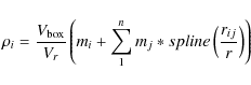
here mj is the mass of particle j (one of i's n closest neighbours), rij is the distance between particles i and j, and is the SPH smoothing length for particle j.
  and Vr
are the volumes of the simulation box and of a sphere of radius r
respectively, so their ratio yields the normalisation of the density
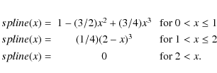
across the box. The spline function is the
well-known Smoothed Particle Hydrodynamics (SPH) kernel:
and Vr
are the volumes of the simulation box and of a sphere of radius r
respectively, so their ratio yields the normalisation of the density
across the box. The spline function is the
well-known Smoothed Particle Hydrodynamics (SPH) kernel:
- 2.
- Walking from particle to particle, identify local maxima
throughout the density field. Apply a first density threshold
 (which roughly corresponds to b =0.2 used as
standard by the FOF algorithm) to all particles, and link particles
with a density above
(which roughly corresponds to b =0.2 used as
standard by the FOF algorithm) to all particles, and link particles
with a density above  to their closest local maximum. These groups of particles are defined
as (sub)structures.
to their closest local maximum. These groups of particles are defined
as (sub)structures.
- 3.
- Identify saddle points in the density field between these
groups. Use these saddle points to create branches connecting maxima
together, in order to build a structure tree i.e. a hierarchy of nodes
where each node contains a collection of particles whose associated
density is enclosed between two values. The lowest value is the density
threshold used to create the first node; the highest is the density
associated to the lowest saddle point (if any) detected inside it. The
lowest (``first'') level nodes are created by linking groups together
whose saddle point is above the first threshold .
The node structure tree is then created by sorting groups in ascending
order according to the value of the density associated with their
saddle points.
Whereas we can logically define a AdaptaHOP halo as the
collapsed node structure tree corresponding
to a group of particles above the ![]() density threshold, its decomposition into a main halo and a collection
of subhaloes is more tricky. The main problem lies in the fact that
nodes are not in general associated with physical objects.
Only end-of-chain nodes, i.e. leaves, have a physical meaning, so we
have to re-arrange the node structure tree
in order to build the main halo and the subhaloes.
We tackle this issue in the next subsection (subhalo detection).
density threshold, its decomposition into a main halo and a collection
of subhaloes is more tricky. The main problem lies in the fact that
nodes are not in general associated with physical objects.
Only end-of-chain nodes, i.e. leaves, have a physical meaning, so we
have to re-arrange the node structure tree
in order to build the main halo and the subhaloes.
We tackle this issue in the next subsection (subhalo detection).
![\begin{figure}
\par\includegraphics[width=9cm,clip]{11787f01.eps}
\end{figure}](/articles/aa/full_html/2009/41/aa11787-09/img15.png) |
Figure 1: Example of a node structure tree as computed with AdaptaHOP. Ellipses are nodes. The arrows show relationship between nodes. In a branch of the tree two levels are separated by a saddle point (indicated by a dashed line) in the density profile. Leaves in the node structure tree are shown in grey. More massive leaves are represented by larger circles. Density of nodes decreases from top to bottom. |
| Open with DEXTER | |
2.2 Dark matter subhalo detection: one step methods
These last remarks naturally lead us to address the issue of substructure identification, i.e. the detection of subhaloes within haloes as well as subhaloes within subhaloes. The main problem we are faced with concerns the node structure built with AdaptaHOP and described at the very beginning of the previous section: nodes are not in general associated with physical objects. Only the end-of-chain nodes, i.e. the leaves, have a physical meaning as they are the only true local density maxima in the density profile of their host halo. Since we need to define physical objects as subhaloes, a method is needed to create a tree comprised of a main halo and its subhaloes from the node structure tree computed by AdaptaHOP. We propose several such methods in this section, and compare/contrast their advantages and disadvantages in the next (Merger Histories).
The obvious choice would be to define as subhaloes all the leaves in the node structure tree. Still referring to the example shown in Fig. 1, this means that we would define nodes 5, 6, 7, 8, 9 as subhaloes (shown in grey in this figure) and associate nodes 1, 2, 3 and 4 (in white) to the main halo. However, this method is not very satisfying because it leads to the loss of the hierarchy of subhaloes: we would be left with only 2 levels of structures, making it impossible to account for the presence of a subhalo within another subhalo. Moreover not all density maxima can be defined as subhaloes, as one naturally expects the main halo itself to be centered on a density maximum.
For this reason, one is forced to lay down two simple, intuitive rules to build a halo tree:
- 1.
- the main halo and each of the subhaloes of the halo tree must contain one unique leaf from the node structure tree;
- 2.
- the hierarchy between nodes of the node structure tree must
be turned into a hierarchy of halo, subhaloes, sub-subhaloes etc. i.e.
when a node contains two leaves, one of the leaves is defined as the
subhalo and the other one, together with the node, forms the host
(sub)halo of this subhalo.
![\begin{figure}
\par\includegraphics[width=8cm,clip]{11787f02.eps}
\end{figure}](/articles/aa/full_html/2009/41/aa11787-09/Timg16.png)
Figure 2: Halo tree obtained from the node structure tree shown in Fig. 1 using the DPM method. Haloes and subhaloes are created by collapsing several nodes together. More massive leaves are represented by larger circles. Density of nodes decreases from top to bottom. Nodes and connections removed from the node structure tree are shown with dashed lines.
Open with DEXTER
Arguably, the most natural thing consists in building this
halo tree by collapsing the node structure tree along a branch
containing the most dense leaf:
the particles contained in this leaf are (arbitrarily) chosen to be
part of the main halo itself, along with all the particles contained in
the lower node levels in which the leaf is included, until we reach the
first node (lowest level). We then define subhaloes by repeating this
procedure for the second most dense leaf, and so on and so forth, until
all leaves have been accounted for. We call this method the Density
Profile Method (DPM) and illustrate how it works in Fig. 2, which is to
be compared
to Fig. 1
depicting the original tree node structure. As node 8 is the leaf with
the highest density, and is spatially included
in node 4, itself being included in node 3, itself being included in
node 1, we simplify the tree node by collapsing branch 8-4-3-1 into a
single, main halo (
![]() ), and replace solid lines and
arrows around nodes 8, 4, 3 with dashes in Fig. 2 to mark that
their particles are now part of a unique object. Note that the centre
of the main halo is therefore located in
leaf 8. Moving on to the second highest density leaf 9, we find that it
is
now only included in node 1 since nodes 3 and 4 have been removed, and
therefore we have to count it as a subhalo of halo (
), and replace solid lines and
arrows around nodes 8, 4, 3 with dashes in Fig. 2 to mark that
their particles are now part of a unique object. Note that the centre
of the main halo is therefore located in
leaf 8. Moving on to the second highest density leaf 9, we find that it
is
now only included in node 1 since nodes 3 and 4 have been removed, and
therefore we have to count it as a subhalo of halo (
![]() ).
Leaf 7 comes next, which is contained in node 2 which is itself
included in the main halo: we therefore collapse the branch starting
from leaf 7 into
a unique subhalo (
).
Leaf 7 comes next, which is contained in node 2 which is itself
included in the main halo: we therefore collapse the branch starting
from leaf 7 into
a unique subhalo (![]() )
of halo (
)
of halo (
![]() ). Leaf 6 is spatially
included in this new (
). Leaf 6 is spatially
included in this new (![]() )
subhalo, it is therefore a subhalo of this subhalo. Finally, leaf 5
stands alone in halo (
)
subhalo, it is therefore a subhalo of this subhalo. Finally, leaf 5
stands alone in halo (
![]() )
since we removed node 3: it becomes yet another of its subhaloes.
It is obvious that this solution follows the two rules we layed out for
defining haloes and subhaloes as objects with different levels in the
structure tree because each of the main halo (
)
since we removed node 3: it becomes yet another of its subhaloes.
It is obvious that this solution follows the two rules we layed out for
defining haloes and subhaloes as objects with different levels in the
structure tree because each of the main halo (
![]() )
on level 1, its three subhaloes (9,
)
on level 1, its three subhaloes (9,![]() ,5) on level 2, and the unique
sub-subhalo (6) on level 3, contain a single leaf from the original
node tree.
,5) on level 2, and the unique
sub-subhalo (6) on level 3, contain a single leaf from the original
node tree.
Moreover, from this simple example, we can easily understand
how changing the criterion to pick the first leaf - for example picking
the most massive one instead of the most dense -, we would have defined
![]() as the main
halo , and found it had two subhaloes,
as the main
halo , and found it had two subhaloes, ![]() ,
and 6. Finally, instead of having node 6 as the only level 3 structure
of the halo structure three, both leaves 5 and 9 would be subhaloes of
subhalo
,
and 6. Finally, instead of having node 6 as the only level 3 structure
of the halo structure three, both leaves 5 and 9 would be subhaloes of
subhalo ![]() .
We call this second method the Most massive Sub-node Method (MSM).
A fundamental difference between halo trees built using DPM and MSM is
that the centre of the main halo is now located in leaf 7 (MSM) instead
of leaf 8 (DPM).
We also emphasise that the criterion used to group nodes to form haloes
and subhaloes has an effect not only on the mass of the main halo but
on the hierarchy (level number) of subhaloes as well.
.
We call this second method the Most massive Sub-node Method (MSM).
A fundamental difference between halo trees built using DPM and MSM is
that the centre of the main halo is now located in leaf 7 (MSM) instead
of leaf 8 (DPM).
We also emphasise that the criterion used to group nodes to form haloes
and subhaloes has an effect not only on the mass of the main halo but
on the hierarchy (level number) of subhaloes as well.
2.2.1 Individual examples
Both methods are then run on the same N-body
simulation described in paper GalICS I (Hatton et al. 2003).
This simulation contains 2563 particles of ![]()
![]() enclosed in a volume
of 150 comoving Mpc on a side, with periodic boundary conditions.
Values for cosmological parameters are given in Table 1.
enclosed in a volume
of 150 comoving Mpc on a side, with periodic boundary conditions.
Values for cosmological parameters are given in Table 1.
Table 1: Simulation details.
We now present two example of haloes using the MSM method to define halos and their hierarchy of subhaloes. Our goal is to check by eye (arguably the best tool to do the job) that we can detect all the subhaloes.
![\begin{figure}
\par\includegraphics[width=9cm,clip]{11787f03.eps}
\end{figure}](/articles/aa/full_html/2009/41/aa11787-09/img25.png) |
Figure 3: Top left: original AdaptaHOP halo with subhaloes, top right: main (MSM) halo (without subhaloes), bottom right: subhaloes, bottom left: circles marking the ``virial'' region of the halo and its subhaloes. |
| Open with DEXTER | |
![\begin{figure}
\par\includegraphics[width=9cm,clip]{11787f04.eps}
\end{figure}](/articles/aa/full_html/2009/41/aa11787-09/img26.png) |
Figure 4: Top left: original AdaptaHOP halo with subhaloes, top right: main (MSM) halo (without subhaloes), bottom left: subhaloes of the main halo, bottom right: subhaloes of the subhaloes. |
| Open with DEXTER | |
As shown in Fig. 3,
the MSM can detect subhaloes quite
well, for a quite relaxed halo of mass ![]()
![]() with its 15
subhaloes, and of mass 1014
with its 15
subhaloes, and of mass 1014 ![]() without them.
It is able to neatly remove all subhaloes as shown in the top right
panel: no spurious holes appear in the density field where these
subhaloes have been removed. The main halo (top right panel) has a
smooth profile even though the
subhaloes shown on the bottom left panel come in various shapes and
sizes. Most of the subhaloes shown here have the main halo as
host. It is easier to observe the size of the various subhaloes by
drawing their
``virial'' region (defined here as a sphere centered on the centre of
the halo or
subhalo and whose radius is such that the average density is
without them.
It is able to neatly remove all subhaloes as shown in the top right
panel: no spurious holes appear in the density field where these
subhaloes have been removed. The main halo (top right panel) has a
smooth profile even though the
subhaloes shown on the bottom left panel come in various shapes and
sizes. Most of the subhaloes shown here have the main halo as
host. It is easier to observe the size of the various subhaloes by
drawing their
``virial'' region (defined here as a sphere centered on the centre of
the halo or
subhalo and whose radius is such that the average density is ![]() )
which are shown on the bottom left panel.
)
which are shown on the bottom left panel.
More revealing is how MSM performs when the halo is still
perturbed by a major
merger with another object (i.e. when the mass ratio between the
two haloes is higher than 1:3). Such a case is detailed in
Fig. 4.
The mass of the AdaptaHOP halo (with subhaloes) is ![]()
![]() ,
but this time
the mass of the main (MSM) halo is only
,
but this time
the mass of the main (MSM) halo is only ![]()
![]() ,
i.e. its 23 subhaloes
contain slightly more mass than it does. Moreover, since one of the
subhaloes is about the same size as the main halo we can expect it to
contain quite a few subhaloes itself.
Indeed, we are not disappointed: as shown in the top right panel of the
figure, the main halo even harbours a plume of low density particles
whose origins probably lie in the tidal stripping of material between
the bigger
subhalo and the host halo. As expected the biggest subhalo hosts a few
subhaloes of its own,
which are large and dense enough to be seen in the bottom right panel
of Fig. 4.
Usually level 3 subhaloes are much smaller and more difficult
to spot on these kind of plots, but the main conclusion is that the MSM
method seems to perform well independently of the state of relaxation
of the AdaptaHOP halo.
,
i.e. its 23 subhaloes
contain slightly more mass than it does. Moreover, since one of the
subhaloes is about the same size as the main halo we can expect it to
contain quite a few subhaloes itself.
Indeed, we are not disappointed: as shown in the top right panel of the
figure, the main halo even harbours a plume of low density particles
whose origins probably lie in the tidal stripping of material between
the bigger
subhalo and the host halo. As expected the biggest subhalo hosts a few
subhaloes of its own,
which are large and dense enough to be seen in the bottom right panel
of Fig. 4.
Usually level 3 subhaloes are much smaller and more difficult
to spot on these kind of plots, but the main conclusion is that the MSM
method seems to perform well independently of the state of relaxation
of the AdaptaHOP halo.
2.2.2 Density vs. mass criteria
At this point, we have to decide which of the two methods is the best suited to reach the goal that we set for ourselves at the beginning of this paper: to build the most reliable (sub)halo merging history tree possible. Is it the DPM, where each subhalo has a lower peak density than its host? Or is it the MSM where each subhalo is less massive than its host? We now compare these two methods.
![\begin{figure}
\par\includegraphics[width=9cm,clip]{11787f05.eps}
\end{figure}](/articles/aa/full_html/2009/41/aa11787-09/img30.png) |
Figure 5: For both methods DPM (diamonds) and MSM (triangles), the mass functions of haloes, subhaloes of haloes and subhaloes of subhaloes are plotted with solid, short-dashed and long-dashed curves respectively. The error bars correspond to Poisson uncertainty. The vertical dotted line corresponds to the 20 particles detection threshold. |
| Open with DEXTER | |
The mass functions obtained for both DPM (diamonds) and MSM (triangles)
methods at z=0 are represented in Fig. 5. For
each method, the mass function of main haloes (level
1 structures), subhaloes of haloes (level 2 structures) and
subhaloes of subhaloes (level 3 and above structures) are represented
respectively with solid, short-dashed, and long dashed curves
respectively. From the figure it is apparent that the mass functions of
haloes are very similar in both methods, with small differences barely
perceptible to the naked eye. These differences are only due to the
fact that the mass of haloes can vary from one method to the other,
when the most massive and the most dense leaves do not coincide. So
even though the total number of haloes detected at redshift 0 is the
same, the number of main haloes per mass bin is expected to vary
slightly. The same comment holds for the mass function of subhaloes,
except at the high mass end where the difference becomes noticeable and
it seems that slightly less subhaloes of halos are detected with the
MSM method. Differences between methods only become apparent in the
mass function of subhaloes of subhaloes (so called level 3 and above).
Among the 9124 subhaloes detected with both methods we count
2170 subhaloes of subhaloes: 1201 subhaloes detected
with the DPM method and 969 with the MSM method. We believe that these
numbers are large enough to trust that the trend of the DPM always
producing a higher number of subhaloes of subhaloes is real. This is
especially true since it is verified for every mass bin, even if the
number of these subhaloes is small for masses above ![]()
![]() ,
(18 for the DPM, 5 for the MSM), and from these bins alone we would be
hard pressed to draw any conclusion.
,
(18 for the DPM, 5 for the MSM), and from these bins alone we would be
hard pressed to draw any conclusion.
![\begin{figure}
\par\includegraphics[width=9cm,clip]{11787f06.eps}
\end{figure}](/articles/aa/full_html/2009/41/aa11787-09/img32.png) |
Figure 6: For both methods DPM (diamonds) and MSM (triangles), the average number of subhaloes per halo (plain curve), and subhaloes per subhalo (dashed curve vertically translated by 2 dex downwards for clarity) are shown. The error bars correspond to the mean quadratic dispersion. The dotted vertical line corresponds to the 20 particle detection threshold. |
| Open with DEXTER | |
The number of subhaloes per halo or subhalo is another aspect of
substructure selection
methods that is worth quantifying. This data is shown in Fig. 6.
For each method (DPM marked with diamonds and MSM with triangles), we
show here the average number of subhaloes per halo (plain curves) and
the number of subhaloes per subhaloes (dashed curves vertically
translated 2 dex downwards for clarity). Once again, the
average number of subhaloes per halo is nearly the same when using
either the DPM or MSM method. As expected, this number is very low 10-3
at ![]()
![]() .
Haloes of these masses are close to the detection threshold and are
unlikely to host any subhaloes. In both cases, we reach an average
number of at least 1 subhalo per halo from 1013
.
Haloes of these masses are close to the detection threshold and are
unlikely to host any subhaloes. In both cases, we reach an average
number of at least 1 subhalo per halo from 1013 ![]() onwards. Close to 1014
onwards. Close to 1014 ![]() ,
we obtain on average 12 subhaloes per halo. The number of
subhaloes per subhalo follows the same trend, but the difference
between the two methods is more marked in that case, with DPM subhaloes
hosting slightly more subhaloes than MSM subhaloes. This result
confirms the impression we got from the mass function (Fig. 5)
that the number of subhaloes of subhaloes is indeed higher with the DPM
method.
,
we obtain on average 12 subhaloes per halo. The number of
subhaloes per subhalo follows the same trend, but the difference
between the two methods is more marked in that case, with DPM subhaloes
hosting slightly more subhaloes than MSM subhaloes. This result
confirms the impression we got from the mass function (Fig. 5)
that the number of subhaloes of subhaloes is indeed higher with the DPM
method.
![\begin{figure}
\par\includegraphics[width=9cm,clip]{11787f07.eps}
\end{figure}](/articles/aa/full_html/2009/41/aa11787-09/img34.png) |
Figure 7:
For each halo under 1014 |
| Open with DEXTER | |
Coming back to the AdaptaHOP haloes (the haloes originally detected by
AdaptaHOP before subhaloes are removed from them), which, unlike the
main haloes are the same for both methods, we select those for which
the main halo has a different mass in each method and compute the mass
fraction contained in all its subhaloes. By definition this mass
fraction is always smaller than 1 since an AdaptaHOP halo contains all
its subhaloes. The result of this exercise is presented in the top
panels of Fig. 7,
where the average mass fraction for the DPM (diamonds) and the MSM
methods (triangles) (left panel) and the individual values (right
panel) are shown. The mass fraction found in DPM subhaloes is close to
0.5 for the smallest haloes and decreases down to 0.3 near 1013 ![]() ,
to rise again and reach 0.5 at 1014
,
to rise again and reach 0.5 at 1014 ![]() .
The mass fraction in MSM subhaloes follows the same trend but the mass
fraction is always about 0.1 lower. The error bars are smaller as well
for the MSM results and this can be viewed more clearly on the top left
panel: the scatter in mass fraction is more pronounced for the DPM
method.
When using the DPM or MSM method on an AdaptaHOP halo, we obtain the
same number of subhaloes, which is the number of density maxima (leaves
in the node structure tree) minus one that is defined as the center of
the main halo itself. For each of these AdaptaHOP haloes the number of
subhaloes therefore is initially the same. However, when the DPM and
MSM methods differ on the choice of the center leaf, a higher mass
fraction of the AdaptaHOP halo is found in DPM subhaloes than in MSM
subhaloes, which is somewhat expected since MSM picks the most massive
center leaf to define it as part of the main halo. What is more
worrisome, is that looking at the bottom panels of Fig. 7, we
realise that the mass ratio between a subhalo
and the main halo can be greater than one with the DPM method across
the entire mass range spanned by the N-body
simulation. Among the 33718 DPM main haloes with a mass lower than 1014
.
The mass fraction in MSM subhaloes follows the same trend but the mass
fraction is always about 0.1 lower. The error bars are smaller as well
for the MSM results and this can be viewed more clearly on the top left
panel: the scatter in mass fraction is more pronounced for the DPM
method.
When using the DPM or MSM method on an AdaptaHOP halo, we obtain the
same number of subhaloes, which is the number of density maxima (leaves
in the node structure tree) minus one that is defined as the center of
the main halo itself. For each of these AdaptaHOP haloes the number of
subhaloes therefore is initially the same. However, when the DPM and
MSM methods differ on the choice of the center leaf, a higher mass
fraction of the AdaptaHOP halo is found in DPM subhaloes than in MSM
subhaloes, which is somewhat expected since MSM picks the most massive
center leaf to define it as part of the main halo. What is more
worrisome, is that looking at the bottom panels of Fig. 7, we
realise that the mass ratio between a subhalo
and the main halo can be greater than one with the DPM method across
the entire mass range spanned by the N-body
simulation. Among the 33718 DPM main haloes with a mass lower than 1014 ![]() ,
455 differ when using the MSM method. Among these, 93 have a
subhalo-halo mass ratio greater than 1 and 35 greater than 1.5.
This never happens for MSM haloes, which have a maximum subhalo-halo
mass ratio lower than 1 by construction. In the left panel, we see that
this mass fraction is on average lower than 0.7 for the MSM haloes and
much smoother than the DPM curve, with a reduced scatter. It decreases
from 0.7 for the smallest haloes to around 0.2 at
,
455 differ when using the MSM method. Among these, 93 have a
subhalo-halo mass ratio greater than 1 and 35 greater than 1.5.
This never happens for MSM haloes, which have a maximum subhalo-halo
mass ratio lower than 1 by construction. In the left panel, we see that
this mass fraction is on average lower than 0.7 for the MSM haloes and
much smoother than the DPM curve, with a reduced scatter. It decreases
from 0.7 for the smallest haloes to around 0.2 at ![]()
![]() ,
and rises again to reach 0.5 for haloes with masses close to 1014
,
and rises again to reach 0.5 for haloes with masses close to 1014 ![]() .
.
The DPM method (density criteria) and the MSM method (mass criteria) do not differ in most cases as the most massive leaf in the node structure tree generally is the densest as well. However, when they do differ, the hierarchy of subhaloes is modified (we obtain more subhaloes in subhaloes with the DPM method) and the mass ratio between a subhalo and its host halo is also modified. This latter can reach unphysical (greater than unity) values with the DPM method which leads us to use the MSM method as our preferred one step method in the rest of this paper.
Having selected a robust (in the sense that it uses an integral quantity, i.e. the mass, rather than its spatial derivative, i.e. the density) and intuitively satisfying method (MSM haloes are more massive than any of their subhaloes) as well as assessed its ability to describe the instantaneous structure of dark matter haloes and subhaloes (i.e. the analysis of an isolated snapshot of an N-body simulation), we now proceed to study how it fares at capturing their much more complex time evolution.
3 Merger histories
3.1 Constructing a merger tree
Although over the course of a numerical N-body simulation most (sub)haloes lose mass and disappear, it is customary to refer to the ``growth'' of haloes since these mass losses also feed the formation of larger objects. Tracking how and when a (sub)halo acquires its mass is called building a merger history tree for this specific (sub)halo. The further complication with respect to the detection of subhaloes previously discussed is that this mass assembly is a dynamical and continuous process, which is only captured by a finite number of discrete time outputs (typically 50 between redshifts 20 and 0, see e.g. Hatton et al. 2003) of an N-body simulation. This means that time resolution issues superimpose on mass resolution issues that were our sole limitation up to now.
![\begin{figure}
\par\includegraphics[width=8cm,clip]{11787f08.eps}
\end{figure}](/articles/aa/full_html/2009/41/aa11787-09/img36.png) |
Figure 8: In a simplified tree built as described in the text (Sect. 3.1), a subhalo may appear without seemingly having a progenitor. Whenever possible, the simplified merger tree is therefore modified so that the subhalo s(st) in the figure becomes the main son of halo h2(st-1), even though h2(st-1) has given most of its particles to h(st) and not s(st). |
| Open with DEXTER | |
Once again, all the information available to build the merging trees is carried by particles, and more specifically by their belonging to a particular (sub)halo at a given time output st and another one at the previous/subsequent snapshot. In other words, by monitoring the exchange of particles between haloes or subhaloes detected in two consecutive snapshots of an N-body simulation, one can build ``simplified'' merger trees by laying down the following set of rules:
- each (sub)halo i at step st can only have 1 son at step st+1, i.e. fragmentation is not taken into account, hence the ``simplified'' adjective used to describe the merging tree;
- assuming mij is the common mass between a (sub)halo i of mass mi at step st and a (sub)halo j of mass mj at step st+1, the son of i is chosen as the (sub)halo j for which mij/mi is maximal;
- conversely, the (sub)halo i of mass mi at step st is a progenitor of the (sub)halo j of mass mj at step st+1 if, and only if j is the son of i. The main progenitor of j is the (sub)halo i for which the ratio mij/mj is maximal.
In the remaining subsections of the paper we will be talking about tree branches. What we define as a branch is a succession of haloes and subhaloes linked together between two outputs of an N-body simulation by a main progenitor - main son relationship. It means that there is only one (sub)halo per branch at any given step, and that a branch starts with a (sub)halo which has no progenitor and ends (i) when a merger occurs with another branch or (ii) when a (sub)halo has no son at the next output or (iii) when the current output is the last one (e.g. z=0).
3.2 Example of a merger tree built with and without subhaloes
![\begin{figure}
\par\includegraphics[width=9cm,clip]{11787f09.eps}
\end{figure}](/articles/aa/full_html/2009/41/aa11787-09/img38.png) |
Figure 9: Example of a merger tree computed with MSM subhaloes according to the rules described in the text (Sect. 3.1). Circles represent main haloes, squares subhaloes. The main halo at redshift 0 is the one shown in Fig. 3. Its merger tree is shown in the left hand side of the figure, whereas the merger trees of its subhaloes are shown on the right hand side. Main haloes are connected to their subhaloes using horizontal solid lines and mergers between (sub)haloes are indicated by horizontal dotted lines. A mass threshold was applied not to show the less massive (thick) branches and limit this tree to less than 50 branches. Only the 40 most massive branches of the full merger tree are shown in this figure. |
| Open with DEXTER | |
![\begin{figure}
\par\includegraphics[width=9cm,clip]{11787f10.eps}
\end{figure}](/articles/aa/full_html/2009/41/aa11787-09/img39.png) |
Figure 10: Same as Fig. 9 except that the subhaloes have not been taken into account (i.e. it is the merger tree of an AdaptaHOP halo which includes but does not separate subhaloes). A mass threshold was applied so as not to show the less massive (thick) branches and limit this tree to less than 50 branches. Only the 42 most massive branches of the full merger tree are shown in this figure. |
| Open with DEXTER | |
Figure 9 shows the full merger tree of the halo shown in Fig. 3, with subhaloes determined via the MSM, albeit for this particular halo, little difference would occur if this merger tree was constructed with the DPM. In this figure, haloes are represented as circles, subhaloes as squares. The main halo and its subhaloes are on the first line, and all of their progenitors on subsequent lines as time flows from the bottom to the top of the figure. Each column is a branch of the tree either linked to the halo or one of its subhaloes. The main progenitor is always in the same column as its son. When a merger occurs one branch ends (no more objects in this column) and a line connects it to the branch it has merged with. In this plot we show that 16 branches directly lead to the main halo at redshift 0. The first one is the main branch (the trunk), and the 15 other ones which end before redshift 0 are called secondary branches. The other 22 ``sub''-branches define the merger histories of subhaloes hosted by the main halo at redshift 0. The relationships between haloes and subhaloes are indicated by a line at the top of each branch. They show whether a subhalo is hosted by the main halo itself (solid lines connecting the two objects) or, as for the branch in Col. 29, another subhalo (dashed lines connecting the two objects). Some lines linking branches are dotted: these mark mergers between (sub)haloes which resulted in both objects retaining their identities (one becomes the subhalo of the other). When this happens either of two things can occur at later times: (i) the branch of the subhalo merges with the branch of its host or (ii) the subhalo becomes a stand alone halo again. Both cases are present in the halo merger tree of Fig. 9, with case (i) being more frequent (branches in Cols. 2, 3, 7, 8, 9, 10, 15, 27, 28, 31, 32, 33, 35) than case (ii) (branches in Cols. 13, 14, 23, 25, 34). Physically, case (i) corresponds to progressive mass stripping of the subhalo through dynamical friction, and case (ii) to structures which fly by one another several times on elongated orbits before merging together for good.
If we do not keep track of the subhaloes, as shown in Fig. 10 where we plot the merger tree of the AdaptaHOP halo (the halo which includes the main halo and all subhaloes) the same phenomenon of multiple fly-bys before merger leads to branches being cut into pieces. The lower part of the branch will merge with the halo at the first encounter, and the top part of the branch will reappear as a new branch each time the ``subhalo'' jumps down a level in the halo tree, e.g. becomes a halo again if it had become a ``level 2 subhalo'' during the first encounter (branches in Cols. 18 and 20). However, the general impression one gets from glancing at Fig. 10 is that the AdaptaHOP halo merger tree is quite close to the MSM one (Fig. 9). More specifically, if we ignore the squares and replace the dashed lines by solid lines in this figure it is clear that many mergers observed in Fig. 10, are also found in Fig. 9 (branches in Cols. 2 and 3 are identical, branch 4 in Fig. 10 is branch 13 in Fig. 9, and so on and so forth...).
One of the main ideas behind this paper is to construct ``well behaved'' merging trees from N-body simulations, on which we can graft semi-analytic models (SAM: e.g. Hatton et al. 2003; Kauffmann et al. 1999; Roukema et al. 1997) of galaxy formation and evolution on top of them. In order for this to be possible, we expect our trees to be devoid of certain features. For instance, subhaloes should only appear after a merger involving main haloes has taken place. This means that any subhalo should have at least one progenitor. We then expect a subhalo to be either stripped of its mass and merge with its host structure, or become temporarily distinct again (see discussion above). Which means that, in principle, it should not be possible for a subhalo to ever be part of a main branch. A thorough analysis of our merging tree building method(s) therefore leads us to define three types of anomalies that are to be avoided, or at least reduced to a minimum of occurrences:
- 1.
- anomaly of the first kind: a subhalo has no progenitor;
- 2.
- anomaly of the second kind: a subhalo merges with its host but its branch does not end;
- 3.
- anomaly of the third kind: a subhalo swaps identity with its host.
3.3 A two time step method: the branch history method (BHM)
![\begin{figure}
\par\includegraphics[width=8cm,clip]{11787f12.eps}
\end{figure}](/articles/aa/full_html/2009/41/aa11787-09/img41.png) |
Figure 12: Illustration of the BHM method (see text, Sect. 3.3, for details), where a node, n1, and two of its subnodes, sn11 and sn12 at step st, are linked to the progenitors of subnodes (either haloes or subhaloes) at step st-1 (named P11 and P12). |
| Open with DEXTER | |
The occurrence of anomalies in the merger history of haloes is caused by the (poor) finite time resolution necessarily used to store the wealth of information contained in N-body simulations. It therefore seems natural to try to include information coming from various time outputs to get rid of them. In this section, we present a method that uses information over two such time outputs, but it can in principle be extended beyond this (at the expense of computational power and complexity) to build truly ``perfect'', i.e. virtually anomaly free, trees. Like the other methods, the Branch History Method (BHM) starts with the node structure tree computed with AdaptaHOP, but it works in the following way:
- Load the (sub)halo distribution of the previous time output in memory. If there is none (first snapshot), use the MSM method to detect (sub)haloes.
- Construct the halo tree from the highest level of the node structure tree to the lowest one (which is the main halo itself: see Sect. 2 ``structure detection'' for details) for the current time output.
- When a node n1 contains two subnodes sn11 and sn12, check that the mass of (n1 + sn11) is greater that the mass of sn12. Similarly when using sn12 instead of sn11, check that the mass of (n1 + sn12) is greater that the mass of sn11, to ensure that if one of the subnodes is defined as a subhalo, its mass will be lower than that of its host.
- Compute the main progenitor of each of the objects sn11, sn12, (n1 + sn11) and (n1 + sn12), i.e. the halo or subhalo with which these objects have most mass in common at the previous time output. We shall name those progenitors P11,P12,P1+11 and P1+12. See Fig. 12 for illustration.
- Apply the following criteria:
- 1.
- if P11
= P1+11 and
 ,
then sn12 is a subhalo and (n1
+ sn11) its host. Vice versa
if
,
then sn12 is a subhalo and (n1
+ sn11) its host. Vice versa
if  and P12
= P1+12, sn11
is a subhalo and (n1
+ sn12) its host;
and P12
= P1+12, sn11
is a subhalo and (n1
+ sn12) its host;
- 2.
- if P11 = P1+11, P12 = P1+12, and P11 and P12 are both haloes, use the same criteria as the MSM method: if the mass of sn12 is lower than the mass of sn11, then sn12 is a subhalo and (n1 + sn11) its host;
- 3.
- if P11 = P1+11, P12 = P1+12, P11 is a subhalo and P12 a halo then sn11 is a subhalo and (n1 + sn12) its host. Vice versa if P11 is a halo and P12 a subhalo then sn12 is a subhalo and (n1 + sn11) its host: i.e. make sure that a subhalo remains a subhalo whenever possible;
- 4.
- if
and ,
then both sn11 and sn12
are subhaloes and n1 is
their host: the masses of sn11
and sn12 are small compared
to that of n1, so there is
no reason to decide that one subnode is a subhalo and not the other.
![\begin{figure}
\par\includegraphics[width=9cm,clip]{11787f13.eps}
\end{figure}](/articles/aa/full_html/2009/41/aa11787-09/img44.png) |
Figure 13: Percentage per mass bin of subhaloes without progenitor, i.e. of the occurrence of the first anomaly, for the three merging tree building methods described in the text: DPM (diamonds), MSM (triangles), BHM (squares). The error bars correspond to Poisson uncertainties. The vertical dotted line corresponds to the 20 particles detection threshold. |
| Open with DEXTER | |
Figure 13
shows results obtained for the anomaly of the first kind, i.e. the
number of subhaloes for which no progenitor could be assigned. These
results follow the same trend as a function of subhalo mass whatever
the tree building method (DPM, MSM, BHM) used. Up to 26% of the smaller
subhaloes do not have a progenitor but this fraction quickly decreases
as the mass of the subhalo increases, falling below the 10% mark for
DPM, MSM and BHM subhaloes more massive than ![]()
![]() ,
,
![]()
![]() and
and ![]()
![]() respectively. For the DPM, this percentage stays between 5.3 and 4.3%
from
respectively. For the DPM, this percentage stays between 5.3 and 4.3%
from ![]()
![]() to
to ![]()
![]() ,
then decreases below the 3% mark from
,
then decreases below the 3% mark from ![]()
![]() onward. For the MSM and BHM methods the 5% level is reached at
onward. For the MSM and BHM methods the 5% level is reached at ![]()
![]() and
and ![]()
![]() and the 2% mark at
and the 2% mark at ![]()
![]() and
and ![]()
![]() .
In the last mass bin, all methods detect only 1 subhalo with no
progenitor, but since the number of subhaloes is higher in this bin for
the DPM (77 compared to 41 for MSM and BHM) the percentage is slightly
lower for this method.
.
In the last mass bin, all methods detect only 1 subhalo with no
progenitor, but since the number of subhaloes is higher in this bin for
the DPM (77 compared to 41 for MSM and BHM) the percentage is slightly
lower for this method.
We conclude that as far as anomalies of the first kind are
concerned, both the MSM and BHM yield significantly better results, as
their fraction of subhaloes without progenitors is systematically a few
% lower than with the DPM. The fact that 26% of the smallest subhaloes
have no progenitor is not too worrying, as these subhaloes are more
prone to contamination by Poisson noise: they mostly disappear from a
time output to the next simply because they lose a few particles and
drop below the detection threshold of 20 particles. For the
larger subhaloes, the main reason for the anomaly to occur is that a
subhalo with a similar maximal density than its host and coming close
to the center of the latter on a radial orbit can be blended with it![]() . At the time output when
the blending occurs, one then detects just one structure: the host.
This anomaly can be understood as a fly-by process occurring for
subhaloes, also
occurring with the SUBFIND algorithm and detailed by Wetzel et al. (2009).
. At the time output when
the blending occurs, one then detects just one structure: the host.
This anomaly can be understood as a fly-by process occurring for
subhaloes, also
occurring with the SUBFIND algorithm and detailed by Wetzel et al. (2009).
However, at the next time output this need not be the case, and since we do not allow a (sub)halo to have more than one son, a structure is left without a progenitor. Depending on the method one uses to define (sub)haloes, this can happen more (DPM) or less (BHM) often, as different haloes can be picked as main progenitors.
![\begin{figure}
\par\includegraphics[width=9cm,clip]{11787f14.eps}
\end{figure}](/articles/aa/full_html/2009/41/aa11787-09/img54.png) |
Figure 14: For the three merging tree building methods DPM (diamonds), MSM (triangles), BHM (squares), haloes at redshift 0 have been sorted into 15 mass bins. The merger trees of each of these haloes were analysed, to detect occurrences of the anomaly of the second kind, i.e. a subhalo merging with its host halo but becoming the main progenitor of the resulting main halo. For each mass bin, the percentage of trees in which this anomaly occurred at least once is given. The error bars correspond to Poisson uncertainties. The vertical dotted line corresponds to the 20 particles detection threshold. |
| Open with DEXTER | |
![\begin{figure}
\par\includegraphics[width=9cm,clip]{11787f15.eps}
\end{figure}](/articles/aa/full_html/2009/41/aa11787-09/img55.png) |
Figure 15: Same as Fig. 14 but for anomalies of the third kind, i.e. from one step to another, a subhalo is detected in its host halo branch, and the host halo is detected in the subhalo branch. In each bin the number of trees where this anomaly occurred at least once is displayed. The vertical dotted line corresponds to the 20 particles detection threshold. |
| Open with DEXTER | |
In Figs. 14 and 15, we searched the merger trees of each z=0 halo built using all three methods for occurrences of anomalies of the second and third kind respectively. These trees were sorted into 15 mass bins corresponding to the mass of the final halo and its subhaloes at redshift 0, meaning that for all method any tree is in the same bin.
Contrary to the first kind of anomaly, the second kind is
quite scarce. It occurs only in 219, 4 and 31 trees for the DPM, MSM
and BHM respectively.
Looking at the DPM results in Fig. 14, we can
verify that our a priori expectation to detect more anomalies of the
second type when the merger trees become quite complex (i.e. trees of
massive z=0 haloes composed of many branches) is
borne out. For the largest DPM haloes, this anomaly is bound to appear
at least once: the percentage of merger trees containing an anomaly of
the second kind is close to 0 for the smallest haloes, and reaches 100%
for the largest ones. This rise is quite slow until ![]()
![]() where the 10% mark is reached, but quickly accelerates until, from
where the 10% mark is reached, but quickly accelerates until, from ![]()
![]() onward, all DPM trees contain the second kind of anomaly at least once.
With the MSM, the second type of anomaly hardly ever occurs, meaning
that the percentage of trees containing this anomaly is always close to
0, except for the
onward, all DPM trees contain the second kind of anomaly at least once.
With the MSM, the second type of anomaly hardly ever occurs, meaning
that the percentage of trees containing this anomaly is always close to
0, except for the ![]()
![]() mass bin where 1 tree out of 6 contains this anomaly. For the
BHM, until
mass bin where 1 tree out of 6 contains this anomaly. For the
BHM, until ![]()
![]() ,
the percentage of trees containing this anomaly is below 5%.
Interestingly enough, the number of second type anomalies for the BHM
is higher than for the MSM. Around
,
the percentage of trees containing this anomaly is below 5%.
Interestingly enough, the number of second type anomalies for the BHM
is higher than for the MSM. Around ![]()
![]() ,
one third of the trees are plagued with this
anomaly and above
,
one third of the trees are plagued with this
anomaly and above ![]()
![]() this fraction rises to one half. This seemingly dramatic difference
must be somewhat tempered by the small number of events as the two
final mass bins contain eight trees in total. However, we conjecture
that this behaviour of the BHM is the result of the propagation in time
of a small fraction of the much more frequent anomalies of the third
kind. To be more specific, it so happens that the in-built tendency of
the BHM to preserve the level of subhaloes from one output to the next
leads, in some cases, to confuse subhalo
and halo when the branches finally merge together.
this fraction rises to one half. This seemingly dramatic difference
must be somewhat tempered by the small number of events as the two
final mass bins contain eight trees in total. However, we conjecture
that this behaviour of the BHM is the result of the propagation in time
of a small fraction of the much more frequent anomalies of the third
kind. To be more specific, it so happens that the in-built tendency of
the BHM to preserve the level of subhaloes from one output to the next
leads, in some cases, to confuse subhalo
and halo when the branches finally merge together.
As a matter of fact, looking at the occurrence of anomalies of
the third kind displayed in Fig. 15, we notice
that they appear much more frequently than the anomalies of the second
kind (error bars at a given percentage are much smaller than in
Fig. 14).
Here again, as expected,
these anomalies become more frequent as merger trees become more
complex. For the largest haloes, this anomaly is bound to appear at
least once, whatever the method used to build the merger tree. For the
DPM this rise is quite steady, the 50% threshold being reached for
trees with final haloes of mass ![]()
![]()
![]() ,
and from
,
and from ![]()
![]() onward, all trees contain this anomaly at least once. For the MSM
method, the transition is more pronounced, with the fraction of trees
containing the anomaly rising quite slowly until 1013
onward, all trees contain this anomaly at least once. For the MSM
method, the transition is more pronounced, with the fraction of trees
containing the anomaly rising quite slowly until 1013 ![]() ,
reaching the 50% threshold for
,
reaching the 50% threshold for ![]()
![]() haloes, and 100% at
haloes, and 100% at ![]()
![]() .
However, the discrepancy between MSM and BHM is in favour of the latter
this time around: the fraction of trees containing anomalies of the
third kind gently rises from 0 to 20% when final haloes masses attain
.
However, the discrepancy between MSM and BHM is in favour of the latter
this time around: the fraction of trees containing anomalies of the
third kind gently rises from 0 to 20% when final haloes masses attain ![]()
![]() ,
reaches 50% at
,
reaches 50% at ![]()
![]() and 100% at
and 100% at ![]()
![]() .
In other words, the number of trees containing this anomaly is reduced
by a factor 4 on average when going from the MSM to the BHM,
so that the conversion of a few of these anomalies into anomalies of
the second kind seems a small price to pay. Also, we have good reasons
to believe that an extended
BHM over more than two time outputs could definitively resolve the
issue.
.
In other words, the number of trees containing this anomaly is reduced
by a factor 4 on average when going from the MSM to the BHM,
so that the conversion of a few of these anomalies into anomalies of
the second kind seems a small price to pay. Also, we have good reasons
to believe that an extended
BHM over more than two time outputs could definitively resolve the
issue.
The conclusions we can draw from these three anomaly tests are that (i) the method used when creating the halo tree has an important impact on the merger tree (ii) the most obvious anomalies can be avoided by using an MSM like method (iii) further improvement is possible using BHM like methods but it does not reduce all anomalies to the same extent and comes at quite an expensive cost in terms of complexity of algorithm and CPU requirement. In the remaining of the paper we examine how the shape of individual merger trees is affected when one uses these three different tree building methods, illustrating how these differences can affect SAMs which are grafted on the trees.
3.4 Examples of individual merger trees and their consequences in terms of halo formation epoch
We pick merger trees where the three methods DPM, MSM and BHM differ and zoom in on the portion of the tree where these differences take place. For each Figs. 16, 17, 18 the left hand side displays the tree obtained using the DPM, the middle spot is occupied by the MSM tree and the BHM tree is shown on the right hand side. As in the previous plots throughout the paper, haloes are represented by circles and subhaloes by squares, solid lines show relationships between main progenitor and main son, dashed lines stand for mergers where a halo survives as a subhalo and they link the main subhalo progenitor to its new host. For an easier analysis, each branch has been indexed from 1 to 9 (number below each branch).
![\begin{figure}
\par\includegraphics[width=9cm,clip]{11787f16.eps}
\end{figure}](/articles/aa/full_html/2009/41/aa11787-09/img67.png) |
Figure 16: Zoom on merger trees obtained for the same final halo using three methods of subhalo selection. The DPM tree is shown on the left hand side, the MSM tree in the middle and the BHM tree on the right hand side (see text, Sects. 3.1 and 3.3, for detail). Circles represent haloes, squares subhaloes. Solid lines show progenitor-son relationships, dashed lines stand for mergers that resulted in one of the merging haloes surviving as a subhalo. |
| Open with DEXTER | |
The first example (Fig. 16) illustrates the dreadful effect the DPM can have on a merger tree. In the first (main) branch of the DPM tree, we can see an inversion between halo and subhalo (anomaly of the third kind) between branches 1 and 6 around redshift 0.15. Branch 1 also starts awkwardly as a small halo around redshift 3.9, keeps its mass for about seventeen outputs, and suddenly becomes a much larger subhalo around z=1.7 without undergoing an obvious merger. This subhalo should be the remnant of the merger of branch 1 with branch 2, but instead an anomaly of the third kind appears.
The MSM tree for the same halo (middle tree in Fig. 16) behaves in a much more civilised manner: the first (main) branch starts as expected with haloes growing in size regularly from one time output to the next. However, we still find a subhalo in the main branch around redshift 0.2. Looking back at the DPM tree, we can see that this is due to an identification problem with a branch that ends as a subhalo at redshift 0 in the MSM tree but not in the DPM tree (equivalent of DPM branch 6), and for this reason is not shown here (we only plot the merger tree of the main halo for each method). We notice that branch 3 has two merger events with branch 5, leading to its main halo turning into a subhalo for one output on both occasions. Branch 6 merges with branch 7: it is a subhalo-subhalo merger where the resulting subhalo eventually merges with the main branch around redshift 0.5. We can also see that branch 9 starts as a quite large subhalo around redshift 0.8, and thus can be defined as an anomaly of the first kind. Nevertheless, we still conclude that for this halo, the MSM method is better than the DPM as the most obvious anomalies present in the DPM main branch are greatly suppressed by the MSM and
![\begin{figure}
\par\includegraphics[width=9cm,clip]{11787f17.eps}
\end{figure}](/articles/aa/full_html/2009/41/aa11787-09/img68.png) |
Figure 17: Same as Fig. 16, for another halo. |
| Open with DEXTER | |
![\begin{figure}
\par\includegraphics[width=9cm,clip]{11787f18.eps}
\end{figure}](/articles/aa/full_html/2009/41/aa11787-09/img69.png) |
Figure 18: |
| Open with DEXTER | |
The second example proposed in Fig. 17 is also a zoom of a main branch but only from redshift 8 down to redshift 1.4 this time. Once again subhaloes are present in the main branch of the DPM tree as a result of a merger with branch 3 around z=2.4. The subhalo in the MSM main branch at redshift 2, however is due to a type 3 anomaly involving branch 4. This latter is also branch 3 of the DPM tree and the main branch of the BHM tree, which explains why the anomaly disappears in that case. The main branch of the MSM tree can be partly identified with branch 2 of the BHM tree, even though their first haloes (from z=5 to z=3.2) differ. Apart from this, MSM and BHM trees are very similar overall: we can identify branches 2, 7 ,8 and 9 of the MSM tree with branches 3, 6,7 and 9 of the BHM tree.
The last example (Fig. 18) illustrates that the BHM is not entirely fool proof, in the sense that not all anomalies in its merger trees can be eradicated. This example is a zoom on the main branch of a halo between redshifts 1.85 and 0. As we can see in the figure, several subhaloes appear in the main branch of the DPM tree. Their presence is caused by an exchange between haloes and subhaloes first with branch 2 (z=1.85) then with branch 5 (z=0.42). The second occurrence of this anomaly lasts 3 steps. In the MSM tree only one subhalo appears in the main branch. Except for branch 4 that does not appear and branch 3 which is branch 4 in the MSM tree, all the branches have the same index in both DPM and MSM trees.
The first occurrence of the anomaly (between DPM branches 1 and 2) is prevented by going to the MSM method, however one occurrence of an anomaly of the third kind persists between branches 1 and 5. In both cases there is an anomaly of the first kind in branch 8. As these branches broadly have the same thickness, the merger between their haloes is a major one, which explains why the MSM fails. Looking at the main branch of the BHM tree we see that it contains two subhaloes, which is surprising since this result is worse than that obtained with the MSM method. It is, in fact not such an unexpected turn of events: the BHM simply performed as well as the MSM in the first instance when the subhalo appeared due to the major merger between the two haloes. However at the following time output, it took into account the information that the halo of the main branch had become a subhalo and since it was possible, decided to maintain its subhalo status. At the following output, this possibility had vanished, and the subhalo was restored to its main halo status. Another difference between the MSM and the BHM trees is quite noticeable: branch 5 of the BHM tree corresponds to both MSM branches 5 and 8. The BHM method managed to preserve the progenitor-son link of the subhalo involved in the major merger two time outputs further than the MSM.
![\begin{figure}
\par\includegraphics[width=8.5cm,clip]{11787f19.eps}
\end{figure}](/articles/aa/full_html/2009/41/aa11787-09/img70.png) |
Figure 19: Formation and assembly epoch of z=0 main haloes according to the different merging tree building methods described in the text (Sects. 3.1 and 3.3). Dashed (upper) curve shows formation redshift (defined as the redshift when the sum over the mass of all progenitors at a given time output reaches 50% of the final z=0 main halo mass) as a function of halo mass, and solid (lower) curve shows assembly redshift (defined as the redshift where 50% of the mass of the final main halo is assembled in the main branch for the first time). |
| Open with DEXTER | |
Turning to a statistical measure to quantify the impact of using
different methods to build halo merger trees, we now focus on measuring
the ``downsizing/upsizing'' nature of the formation process of dark
matter haloes. This is an important issue for galaxy formation as
observations reveal (e.g. Thomas
et al. 2005) that most massive galaxies, which are
generally located in the most massive DM haloes, are composed of older
stars than their less massive counterparts. Our results are plotted in
Fig. 19
for the 3 different methods we use to build merging trees. There are 2
sets of curves in this figure, the first one (lower curves) showing
what we call the ``redshift of assembly'' (![]() )
as a function of halo mass, and the second one (upper curves) showing
the ``redshift of formation''
(
)
as a function of halo mass, and the second one (upper curves) showing
the ``redshift of formation''
(![]() ).
). ![]() is defined as the redshift when 50% of the mass of the z=0
main halo is assembled in the main branch (the branch of the main
progenitor or trunk) for the first time.
is defined as the redshift when 50% of the mass of the z=0
main halo is assembled in the main branch (the branch of the main
progenitor or trunk) for the first time. ![]() is the redshift at which the sum of the masses of all
progenitors (independent of the branch they are part of) first reach
50% of the mass of the z=0 main halo
is the redshift at which the sum of the masses of all
progenitors (independent of the branch they are part of) first reach
50% of the mass of the z=0 main halo![]() .
.
The first thing to note is that all three methods yield very
similar results with the exception of the formation redshift in the one
before last mass bin, where the different identification of a single
main halo by the methods is blown out of proportion by poor statistics.
It is interesting to compare Fig. 19 to
Fig. 5 of Neistein
et al. (2006), who plot the same quantities for
Monte-Carlo merging trees based on the EPS formalism, as we can use
their calculations to infer the impact of mass resolution on our
results. As these authors point out, for haloes of a few 1011 ![]() at z=0, i.e. close to our resolution limit, the
number of progenitors is small, and the full merger tree is not much
more complex than the main branch. This has two effects we can see: the
values of
at z=0, i.e. close to our resolution limit, the
number of progenitors is small, and the full merger tree is not much
more complex than the main branch. This has two effects we can see: the
values of ![]() and
and ![]() are (i) not very different from one another (ii) artificially drop at
low masses. When the mass gets higher, the scatter in both
are (i) not very different from one another (ii) artificially drop at
low masses. When the mass gets higher, the scatter in both ![]() and
and ![]() slowly decreases, even though it is not so clear from Fig. 19 because
using the main halo instead of the AdaptaHOP halo naturally increases
the dispersion. Finally, whereas
slowly decreases, even though it is not so clear from Fig. 19 because
using the main halo instead of the AdaptaHOP halo naturally increases
the dispersion. Finally, whereas ![]() is very similar,
is very similar, ![]() in Fig. 19
is much lower than the average
in Fig. 19
is much lower than the average ![]() value plotted by Neistein
et al. (2006) in their Fig. 5, peaking at
value plotted by Neistein
et al. (2006) in their Fig. 5, peaking at ![]() instead of
instead of ![]() .
This possibly reflects the fact that our mass resolution is lower than
theirs by two orders of magnitude at 1011
.
This possibly reflects the fact that our mass resolution is lower than
theirs by two orders of magnitude at 1011 ![]() compared to 109
compared to 109 ![]() .
If so, it is very instructive in terms of the impact of mass resolution
on downsizing: if the epoch of half-mass formation is such a sensitive
function of mass resolution as it seems to be, it means that one could
easily be a few billion years off when estimating the mean age of
stellar population of galaxies from a poorly resolved N-body
simulation. We note however that the theoretical estimate these authors
plot in the same figure is flatter and peaks at a lower redshift of
.
If so, it is very instructive in terms of the impact of mass resolution
on downsizing: if the epoch of half-mass formation is such a sensitive
function of mass resolution as it seems to be, it means that one could
easily be a few billion years off when estimating the mean age of
stellar population of galaxies from a poorly resolved N-body
simulation. We note however that the theoretical estimate these authors
plot in the same figure is flatter and peaks at a lower redshift of ![]() ,
in much better agreement with our N-body simulation
results. Obviously this is less of a problem for
,
in much better agreement with our N-body simulation
results. Obviously this is less of a problem for ![]() since this measures the moment when 50% of the mass is assembled in a
unique object which is well resolved as soon as haloes are massive
enough.
since this measures the moment when 50% of the mass is assembled in a
unique object which is well resolved as soon as haloes are massive
enough.
In light of all the tests we have performed, we conclude that the MSM purges merging trees of many of the anomalies which take place when building them with the DPM. This simply confirms that when choosing a subnode to create a halo, one is best advised to use the most massive one instead of the densest. The BHM itself generally yields similar results as the MSM, however the extra information it gleans from the previous time output helps to get rid of most anomalies of the third kind, even though it does propagate an anomaly of the same kind in the tree from time to time. Statistical quantities like the average formation time and the mean redshift of assembly of dark matter haloes are fairly insensitive to the method used to build the trees, but this is less true of the dispersion around this value.
4 Discussion and conclusions
We have presented a comprehensive study of the problems one necessarily encounters when building dark matter halo and subhalo merger trees directly from N-body simulations. We have also suggested methods to greatly reduce them, if not solve them perfectly. To the best of our knowledge, the first trees of this kind were used by De Lucia & Blaizot (2007); Springel et al. (2005) to populate the millennium cosmological simulation with galaxies. However, the issues we have described in this paper are not the main focus of any of these papers, and we strongly believe they needed to be addressed in detail, especially since a lot of recent work has been devoted to comparisons between Monte-Carlo merger trees to the millennium trees (Forero-Romero 2009; Parkinson et al. 2008; Neistein & Dekel 2008).
The first part of the paper was focused on the difference between dark matter (sub)haloes and their properties (mass and number of objects) identified using AdaptaHOP and simple criteria to separate subhaloes from haloes (DPM, MSM). We also demonstrated that whereas the halo mass function is robust to a change in subhalo identification criteria, there exists a relatively important effect of the latter on the estimate of the mass fraction contained in subhaloes. We concluded this study by arguing that, in keeping with the philosophy of using information contained in particle positions only to define haloes and subhaloes, one should use a mass criterion over a density one to split the internal structure of haloes apart.
This ensures not only that subhaloes identified in this way are always less massive than their host, but also that the time evolution of the subhalo (mass loss, encounters with multiple fly-bys) can be better understood. Indeed using subhaloes in merger history trees helps to resolve issues such as halo fragmentation. Massive haloes which would have appeared to have no progenitors at the previous time output can now be traced as well identified subhaloes in most cases. We also pointed out that using subhaloes in the merger history of haloes, apart from the obvious trend to make the merger history trees more complex because they have more branches, have an impact on the merger histories of main haloes, in the sense that different methods to identify subhaloes will yield different merging trees for the main halo as well. Finally, we demonstrated that as the physical meaning of a (sub)halo is linked to the merger history itself, using part of the past merger history of a (sub)halo to construct its future yields the best results of all methods used to build merging history trees.
As far as mass resolution is concerned, while we did not make use of the most resolved simulations available to us, we feel that we were justified in doing so, as the problems we identified will simply be exacerbated when moving to higher resolution simulations. An interesting side issue that mass resolution raises is if/how much merging trees are preserved when it increases. It was beyond the scope of this first paper, but will be the main focus of our next one. We also could have presented results where we varied time resolution (i.e. the number of outputs of the N-body simulation one uses to build the trees) but whilst occurrences of anomalies in the resulting merger trees would have increased with decreasing time resolution, our conclusions as to the best method to be employed to build the trees would stand.
Although we did not comment much about this point in the main body of the text, our work presumably has non-negligible implications on semi-analytic models of galaxy formation and evolution. More specifically, the anomalies which occur in merger trees built using the different methods (DPM, MSM, BHM) will interact with recipes employed to estimate the cooling rate of hot gas and feedback from active galactic nuclei in these models. Whilst this may not be important statistically for the population of galaxies considered as a whole, calculations of properties of specific sub-populations may be sensitive to the issue. In particular, galaxies hosted by massive haloes will very likely suffer as these are the places where these anomalies are most common: we plan to address this question in a future work.
Finally, the main advantage to be gained using trees directly constructed from N-body simulations to graft on SAM of galaxy formation and evolution, is clustering information. Monte-Carlo merging trees not only do not contain position information but they also fail to describe environment effects on low mass halo assembly (Zhu et al. 2006; Reed et al. 2007; Sheth & Tormen 2004; Wechsler et al. 2006). Positioning SAM galaxies within subhaloes allows one to both compute merging timescales more accurately, but also to measure the intra halo correlation functions predicted by the model with great accuracy (Blaizot et al. 2006). These previous statements need to be somewhat toned down since baryons exert a gravitational effect on dark matter and this will very likely impact the survival of subhaloes, however these effects can be quantified using the framework we have developed in this paper and we plan to address the issue in the near future.
AcknowledgementsD.T. acknowledges the support received from the European Science Foundation (ESF) for the activity entitled ``Computational Astrophysics and Cosmology'' (Grant ASTROSIM ref 1974) during his stay at Oxford. We thank C. Rimes, C. Pichon and J. Forero-Romero for useful discussions. Wealso thank the referee for his corrections and comments. Simulations presented in this paper were run at the IDRIS. This work is part of the Horizon project. http://www.projet-horizon.fr/
References
- Aubert, D., Pichon, C., & Colombi, S. 2004, MNRAS, 352, 376 [NASA ADS] [CrossRef]
- Baugh, C. M. 2006, Rep. Progr. Phys., 69, 3101 [NASA ADS] [CrossRef]
- Benson, A. J., Pearce, F. R., Frenk, C. S., Baugh, C. M., & Jenkins, A. 2001, MNRAS, 320, 261 [NASA ADS] [CrossRef]
- Benson, A. J., Kamionkowski, M., & Hassani, S. H. 2005, MNRAS, 357, 847 [NASA ADS] [CrossRef]
- Blaizot, J., Szapudi, I., Colombi, S., et al. 2006, MNRAS, 369, 1009 [NASA ADS] [CrossRef]
- Bond, J. R., Cole, S., Efstathiou, G., & Kaiser, N. 1991, ApJ, 379, 440 [NASA ADS] [CrossRef]
- Davis, M., Efstathiou, G., Frenk, C. S., & White, S. D. M. 1985, ApJ, 292, 371 [NASA ADS] [CrossRef]
- De Lucia, G., & Blaizot, J. 2007, MNRAS, 375, 2 [NASA ADS] [CrossRef]
- Diemand, J., Kuhlen, M., & Madau, P. 2006, ApJ, 649, 1 [NASA ADS] [CrossRef]
- Dunkley, J., Spergel, D. N., Komatsu, E., et al. 2009, ApJ, 701, 1804 [NASA ADS] [CrossRef]
- Eisenstein, D. J., & Hut, P. 1998, ApJ, 498, 137 [NASA ADS] [CrossRef]
- Fakhouri, O., & Ma, C.-P. 2008, MNRAS, 386, 577 [NASA ADS] [CrossRef]
- Forero-Romero, J. E. 2009, MNRAS, 1094
- Gelb, J. M., & Bertschinger, E. 1994, ApJ, 436, 467 [NASA ADS] [CrossRef]
- Ghigna, S., Moore, B., Governato, F., et al. 1998, MNRAS, 300, 146 [NASA ADS] [CrossRef]
- Gill, S. P. D., Knebe, A., & Gibson, B. K. 2004, MNRAS, 351, 399 [NASA ADS] [CrossRef]
- Hatton, S., Devriendt, J. E. G., Ninin, S., et al. 2003, MNRAS, 343, 75 [NASA ADS] [CrossRef]
- Helly, J. C., Cole, S., Frenk, C. S., et al. 2003, MNRAS, 338, 903 [NASA ADS] [CrossRef]
- Huchra, J. P., & Geller, M. J. 1982, ApJ, 257, 423 [NASA ADS] [CrossRef]
- Kauffmann, G., Colberg, J. M., Diaferio, A., & White, S. D. M. 1999, MNRAS, 303, 188 [NASA ADS] [CrossRef]
- Klypin, A., Gottlöber, S., Kravtsov, A. V., & Khokhlov, A. M. 1999, ApJ, 516, 530 [NASA ADS] [CrossRef]
- Knollmann, S. R., & Knebe, A. 2009, ApJS, 182, 608 [NASA ADS] [CrossRef]
- Lacey, C., & Cole, S. 1994, MNRAS, 271, 676 [NASA ADS]
- Maciejewski, M., Colombi, S., Alard, C., Bouchet, F., & Pichon, C. 2009a, MNRAS, 393, 703 [NASA ADS] [CrossRef]
- Maciejewski, M., Colombi, S., Springel, V., Alard, C., & Bouchet, F. R. 2009b, MNRAS, 396, 1329 [NASA ADS] [CrossRef]
- Nagashima, M., Yahagi, H., Enoki, M., Yoshii, Y., & Gouda, N. 2005, ApJ, 634, 26 [NASA ADS] [CrossRef]
- Neistein, E., & Dekel, A. 2008, MNRAS, 383, 615 [NASA ADS]
- Neistein, E., van den Bosch, F. C., & Dekel, A. 2006, MNRAS, 372, 933 [NASA ADS] [CrossRef]
- Okamoto, T., & Habe, A. 2000, PASJ, 52, 457 [NASA ADS]
- Parkinson, H., Cole, S., & Helly, J. 2008, MNRAS, 383, 557 [NASA ADS]
- Pfitzner, D. W., & Salmon, J. K. 1996, Parallel halo finding in N-body cosmology simulations
- Reed, D. S., Bower, R., Frenk, C. S., Jenkins, A., & Theuns, T. 2007, MNRAS, 374, 2 [NASA ADS] [CrossRef]
- Roukema, B. F., Quinn, P. J., Peterson, B. A., & Rocca-Volmerange, B. 1997, MNRAS, 292, 835 [NASA ADS]
- Sheth, R. K., & Lemson, G. 1999, MNRAS, 305, 946 [NASA ADS] [CrossRef]
- Sheth, R. K., & Tormen, G. 2004, MNRAS, 350, 1385 [NASA ADS] [CrossRef]
- Somerville, R. S., & Primack, J. R. 1999, MNRAS, 310, 1087 [NASA ADS] [CrossRef]
- Springel, V., White, S. D. M., Tormen, G., & Kauffmann, G. 2001, MNRAS, 328, 726 [NASA ADS] [CrossRef]
- Springel, V., White, S. D. M., Jenkins, A., et al. 2005, Nature, 435, 629 [NASA ADS] [CrossRef]
- Thomas, D., Maraston, C., Bender, R., & Mendes de Oliveira, C. 2005, ApJ, 621, 673 [NASA ADS] [CrossRef]
- Wechsler, R. H., Zentner, A. R., Bullock, J. S., Kravtsov, A. V., & Allgood, B. 2006, ApJ, 652, 71 [NASA ADS] [CrossRef]
- Wetzel, A. R., Cohn, J. D., & White, M. 2009, MNRAS, 395, 1376 [NASA ADS] [CrossRef]
- Zhu, G., Zheng, Z., Lin, W. P., et al. 2006, ApJ, 639, L5 [NASA ADS] [CrossRef]
Online Material
Appendix A: Comparing halo finders: AdaptaHOP and FOF
We first proceed in Sect. A.1 of this appendix to compare AdaptaHOP haloes as defined at the end Sect. 2.1 to haloes identified using the popular FOF algorithm with a standard value of b=0.2for the linking length parameter. To be consistent, we also choose 20 as the minimum number of particles a halo detected by the FOF algorithm can contain. The halo finder algorithms are then run on the same N-body simulation described in paper GalICS I (Hatton et al. 2003). We also find necessary to compare the haloes and subhaloes obtained with AdaptaHOP using the MSM method to the halos detected using the FOF algorithm, this task is summarised in Sect. A.2.
A.1 Comparing halos
A.1.1 Individual examples
Our first goal is to ``calibrate'' AdaptaHOP. To do so, we simply
collapse the node structure tree onto its first node to define a single
halo as a group of particles with a density above the ![]() threshold.
threshold.
In this appendix we refer to objects detected with AdaptaHOP and whose hierarchy of inner local density maxima has been collapsed as described in Sect. 2.1 as AdaptaHOP haloes. Similarly FOF haloes are objects detected using the FOF algorithm.
Intuitively, we expect haloes detected with FOF and AdaptaHOP to resemble one another, provided they are fairly relaxed and well resolved, i.e. they are close to spherical in shape and contain a large enough number of particles. This is the case for the halo represented in Fig. A.1. The projected positions of dark matter particles belonging to this halo in the (xy) plane are shown in both panels of this figure, with the centre of the halo located at point (0,0). On the left hand side panel we can see the FOF halo, on the right hand side panel, we can see the AdaptaHOP halo. At first glance, one can easily be convinced that they are mostly the same halo, but, looking a bit closer, one gets the impression that the AdaptaHOP halo contains a few small overdensities which are not included in the FOF halo.
This impression is confirmed by going to the next halo example displayed in Fig. A.2. This one is ``peanut'' shaped as it has just undergone a merger. Again both haloes are quite similar but the AdaptaHOP halo clearly shows overdensities which are not part of the FOF halo.
From these two examples, we conclude that haloes detected by the two algorithms do not seem to be very sensitive to the dynamical state the halo is in. This is understandable since both methods rely on particle positions only to define haloes. However, the smoothing process used by algorithms which compute the density field (AdaptaHOP in our case) seems responsible for the systematic inclusion of more overdensities within the haloes than percolation algorithms (FOF here), especially when haloes are less relaxed. Even though this last point seems minor, it is more important than it seems: if we wished to compare the SUBFIND and AdaptaHOP subhalo distribution for instance, SUBFIND would not detect these extra AdaptaHOP overdensities since it performs a FOF first step, and this would, in turn, influence the computation of the potential energy of the particles that SUBFIND performs, possibly resulting in a different stripping of particles not bound to the halo.
A.1.2 Comparing halo finders: statistics
![\begin{figure}
\par\includegraphics[width=9cm,clip]{11787fA1.eps}
\end{figure}](/articles/aa/full_html/2009/41/aa11787-09/img76.png) |
Figure A.1: Example of a ``relaxed'' halo detected in our test simulation, the left panel is the halo detected using friend-of-friend (FOF) algorithm, the right panel is the same halo detected using AdaptaHOP. The left panel corresponds to the example shown in the top right panel of Fig. 3 before the subhalo decomposition of the AdaptaHOP halo. |
| Open with DEXTER | |
![\begin{figure}
\par\includegraphics[width=9cm,clip]{11787fA2.eps}
\end{figure}](/articles/aa/full_html/2009/41/aa11787-09/img77.png) |
Figure A.2: Example of a ``merging'' halo detected in our test simulation, the left panel is the halo detected using friend-of-friend (FOF) algorithm, the right panel is the same halo detected using AdaptaHOP. The left panel corresponds to the example shown in the top right panel of Fig. 4 before the subhalo decomposition of the AdaptaHOP halo. |
| Open with DEXTER | |
![\begin{figure}
\par\includegraphics[width=9cm,clip]{11787fA3.eps}
\end{figure}](/articles/aa/full_html/2009/41/aa11787-09/img78.png) |
Figure A.3: For both halo finders, haloes detected at redshift 0 were sorted into 25 mass bins. The top panel shows the number of haloes detected with FOF (triangles) and AdaptaHOP (squares) in each mass bin. Using their particle content, we then cross-identify FOF haloes with their AdaptaHOP counterparts, as described in the text (Sect. 2.1.3). In other words, we enforce that each FOF halo is identified with at most one AdaptaHOP halo and that the identification yields the same result when performed in the reverse order. The bottom panel displays the percentage of haloes per mass bin thus cross identified. The error bars correspond to Poisson uncertainties. The vertical dotted line present on both panels corresponds to the 20 particle detection threshold. |
| Open with DEXTER | |
The two individual halo examples discussed in the previous section naturally lead us to wonder about how general the conclusions we have drawn really are. In other words:
- How well does the mass distribution of resolved haloes obtained with both halo finders agree?
- How frequent is the splitting of single AdaptaHOP haloes into several FOF haloes? Does it depend on resolution/mass? Are all pieces detected?
- How do the smallest, poorly resolved, AdaptaHOP and FOF halo (which do not show internal overdensities) populations compare?
To compare FOF haloes to their AdaptaHOP counterparts, we
simply use the list of particles belonging to each halo as follows:
(i) an AdaptaHOP halo is identified with at most one FOF halo, the one
which contains the highest fraction of its particles (ii) the same
procedure is applied to identify a FOF halo to its one and only
AdaptaHOP counterpart. A FOF halo and its AdaptaHOP counterpart are
then deemed to be the same object when both the highest fraction of the
AdaptaHOP halo particles are found in the FOF halo, and the highest
fraction of the FOF halo particles are found in the AdaptaHOP halo. For
each mass bin we then compute the number of haloes which are found to
be ``identical'' in that sense. The curves in the bottom panel are
obtained by dividing this number by the number of FOF haloes in the bin
(triangles) or by the number of AdaptaHOP haloes in the bin (square),
for each mass bin. This yields the percentage of haloes from each
algorithm (FOF or AdaptaHOP) also identified as single haloes by the
other. In the case of the least resolved haloes, 90% of AdaptaHOP
haloes are identified as FOF haloes, but this percentage drops to 77%
for FOF haloes identified as AdaptaHOP haloes. Also in the former case,
the percentage hits the 100% mark from ![]()
![]() onward, whereas for the latter the percentage rises more slowly,
reaching 90% for haloes around
onward, whereas for the latter the percentage rises more slowly,
reaching 90% for haloes around ![]()
![]() ,
and 100% for haloes of 1014
,
and 100% for haloes of 1014 ![]() only.
only.
![\begin{figure}
\par\includegraphics[width=9cm,clip]{11787fA4.eps}
\end{figure}](/articles/aa/full_html/2009/41/aa11787-09/img81.png) |
Figure A.4: Percentage per bin (of width 1 particle) of haloes with less than 50 particles which are not detected in two consecutive snapshots between redshifts 0 and 10, i.e. among a total of 70 snapshots. The error bars correspond to Poisson uncertainties. The vertical dotted line corresponds to the 20 particle detection threshold. |
| Open with DEXTER | |
Whilst one can argue that the comparison of the two algorithms is irrelevant in a regime where results should not be trusted because of a too small number of particles per halo, we believe it is nevertheless important for two reasons: (i) it better underlines the differences between the algorithms and (ii) semi-analytic models of galaxy formation do populate such low resolution haloes with galaxies (e.g. Hatton et al. 2003; Springel et al. 2005). The consequent discrepancy at the low mass end is quite worrisome, and while it is well known that all halo finders will be incomplete when the number of neighbours used to smooth the density field is close to the minimum number of particles per halo, one may wonder whether a significant fraction of these haloes is in any case marginally bound.
A good indicator of this (other than the measure of the total energy of the halo which has quite a large error bar attached to it) is their stability in time. This data is shown in Fig. A.4. We find that 27% of the haloes containing 20 particles detected by FOF at a given time output are not found at the next. This number drops to 17% for AdaptaHOP haloes. For both halo finders this fraction decreases quickly when the number of particles per halo increases. In other words, when using the FOF, we need to reach a resolution of at least 34 particles to lose less than 1% of the haloes between time outputs. In the case of AdaptaHOP, with a resolution of 24 particles or more, less than 1% of haloes are lost. From these numbers, we conjecture that only a small part of the discrepancy between the two algorithms at the low mass end of the halo mass function comes from the fact that AdaptaHOP (and in general algorithms using density criteria) is more efficient than FOF (i.e. algorithms using percolation criteria) for selecting bound objects.
![\begin{figure}
\par\includegraphics[width=9cm,clip]{11787fA5.eps}
\end{figure}](/articles/aa/full_html/2009/41/aa11787-09/img82.png) |
Figure A.5: Every FOF halo detected at redshift 0, with less than 100 particles, is identified with its AdaptaHOP counterpart using the method described in the text (Sect. 2.1.3). Solid curves show the case where we enforce that a unique FOF halo (the one which contains the largest number of particles of its AdaptaHOP counterpart) be identified with its best AdaptaHOP counterpart (the one which contains the highest fraction of the FOF halo particles), as in Fig. A.3. Dashed curves show what happens when we relax this constraint, and allow several FOF haloes to be identified with the same AdaptaHOP counterpart. The error bars correspond to Poisson uncertainties. The vertical dotted line corresponds to the 20 particles detection threshold. |
| Open with DEXTER | |
To further substantiate this claim, we now proceed to check the other possible source of discrepancy, i.e. we address the issue of how many of the smallest FOF haloes are not identified as individual haloes by AdaptaHOP, but simply detected as parts of other (larger) haloes. We therefore apply the same technique we used to produce Fig. A.3 but only to FOF haloes with less than 100 particles since we are interested in the low mass end, and relaxing the constraint that an AdaptaHOP halo must necessarily have a unique FOF counterpart.
Results of this experiment are shown as dotted curves in Fig. A.5. Examination of this figure reveals that:
- when the constraint of unicity is enforced (solid curve),
the percentage of FOF haloes identified as individual AdaptaHOP haloes
never reaches 100%, even for haloes containing 100 particles.
Instead, this percentage rises slowly from 68% for FOF haloes in the
first (20-24 particles) mass bin to reach 90% (+/-1%) for FOF
haloes more massive than

 (44 particles or so);
- when the constraint of unicity is relaxed (dashed curve) -
meaning that one AdaptaHOP halo can have several FOF counterparts -,
only 14% of FOF haloes in the first mass bin (20-24 particles)
are not identified at all by AdaptaHOP as being part of a halo, and
this percentage drops to less than 1% in the next mass bin
(24-28 particles). Furthermore, from a FOF halo mass of
 (32 particles) onward, not a single FOF halo remains undetected by
AdaptaHOP.
(32 particles) onward, not a single FOF halo remains undetected by
AdaptaHOP.
![\begin{figure}
\par\includegraphics[width=9cm,clip]{11787fA6.eps}
\end{figure}](/articles/aa/full_html/2009/41/aa11787-09/img84.png) |
Figure A.6: Average number of FOF haloes at redshift 0 per AdaptaHOP halo. The error bars correspond to the mean quadratic dispersion. The vertical dotted line corresponds to the 20 particles detection threshold. The diamond and the square correspond to the 2 example haloes shown in Figs. A.1 and A.2 respectively. |
| Open with DEXTER | |
One cannot help to wonder how mass dependent such a statement
is, i.e. if these small haloes preferentially get included in the
outskirts of large clusters, or if their ``mis''-classification happens
uniformly across the whole halo mass range spanned by the N-body
simulation. This information is presented in Fig. A.6, where
we counted the number of FOF haloes detected at the last time output (z=0)
inside
each halo found by AdaptaHOP. The AdaptaHOP halo population was then
split into 25 mass bins, and for each of these bins we computed the
average number (and associated mean quadratic dispersion) of FOF haloes
detected as counterparts of the AdaptaHOP haloes. For smallish, galaxy
size AdaptaHOP haloes (less massive than ![]()
![]() or about 400 particles), we find that the average number of
FOF haloes per AdaptaHOP halo stays close to the minimal value of one,
but starts increasing quite steeply as a function of AdaptaHOP halo
mass after that, scaling as
or about 400 particles), we find that the average number of
FOF haloes per AdaptaHOP halo stays close to the minimal value of one,
but starts increasing quite steeply as a function of AdaptaHOP halo
mass after that, scaling as ![]() .
This implies that cluster size haloes detected by AdaptaHOP
with masses comprised between 1014 and 1015
.
This implies that cluster size haloes detected by AdaptaHOP
with masses comprised between 1014 and 1015 ![]() contain up to several tens of
FOF haloes. Since the halo mass function decays as
contain up to several tens of
FOF haloes. Since the halo mass function decays as ![]() (see Fig. A.3)
in this mass range, this means that cluster size AdaptaHOP haloes get
in total roughly the same number of small ``undetected'' FOF haloes as
galaxy/group size AdaptaHOP haloes, only they are redistributed over a
smaller number of objects. As an illustration of the scatter around the
average value, the two example haloes of similar masses displayed in
Figs. A.1
and A.2
are marked with a diamond and a square in Fig. A.6 respectively,
with the diamond AdaptaHOP halo containing 3 FOF haloes and the square
one 16. Note that this explains why in those two cases, most, if not
all the extra ``clumps'' of particles seen in the AdaptaHOP halo are
not present in the FOF halo to which it was identified, but are
detected by FOF as stand alone haloes.
(see Fig. A.3)
in this mass range, this means that cluster size AdaptaHOP haloes get
in total roughly the same number of small ``undetected'' FOF haloes as
galaxy/group size AdaptaHOP haloes, only they are redistributed over a
smaller number of objects. As an illustration of the scatter around the
average value, the two example haloes of similar masses displayed in
Figs. A.1
and A.2
are marked with a diamond and a square in Fig. A.6 respectively,
with the diamond AdaptaHOP halo containing 3 FOF haloes and the square
one 16. Note that this explains why in those two cases, most, if not
all the extra ``clumps'' of particles seen in the AdaptaHOP halo are
not present in the FOF halo to which it was identified, but are
detected by FOF as stand alone haloes.
The two group finding algorithms we have studied (FOF and AdaptaHOP) give similar results. The discrepancies measured between them occur principally at the low mass end of the halo mass function and can be brought down to the percent level when one considers that haloes detected using AdaptaHOP generally contain several FOF haloes. Alternatively, one could use (as in the HOP algorithm, see Eisenstein & Hut 1998), multiple/adaptive density thresholds to separate haloes from the background to reduce discrepancies with percolation algorithms. However it is unclear that the various thresholds to use can be determined using physical arguments, so we believe it makes more sense to limit the number of ``free'' parameters and use a single density threshold, as implemented in AdaptaHOP. One can then take advantage of the embedded hierarchy of density maxima within each of the haloes identified that way to define subhaloes. Finally, we emphasise that it is hard to decide which of the algorithms (percolation or density based) is closer to the ``true'' gravitationally bound halo, as poorly resolved substructures located in the outskirts of massive haloes are neither isolated, nor fully relaxed objects, and as such, a reliable estimate of their total energy is not easy to achieve, making it very difficult to decide whether they are bound to the larger halo.
A.2 Comparing halo finder MSM vs. FOF
A.2.1 Individual example
![\begin{figure}
\par\includegraphics[width=9cm,clip]{11787fA7.eps}
\end{figure}](/articles/aa/full_html/2009/41/aa11787-09/img88.png) |
Figure A.7: Top right panel: AdaptaHOP halo shown in the right panel of Fig. A.2. Top left panel: the 16 FOF haloes whose particles are found in this AdaptaHOP halo (the best FOF halo match is shown in the left panel of Fig. A.2). Bottom left panel: virial regions of the 16 FOF haloes. Bottom right panel: virial regions of the MSM halo and subhaloes as detailed in Fig. 4. |
| Open with DEXTER | |
As mentioned in the previous subsection of this appendix, by mapping particles contained in an AdaptaHOP halo onto the FOF halo distribution, one realises that these particles often belong to several FOF haloes. This is illustrated in Fig. A.7, where we see in the top left panel the 16 FOF haloes which contain particles from the single AdaptaHOP halo plotted in the top right panel. Recall that this means that for each of these 16 FOF haloes most of their particles are cross identified as particles belonging to the AdaptaHOP halo. Each circle in the bottom left panel represents the virial sphere of one of these 16 FOF haloes. The circles on the bottom right panel represent the virial sphere of the main halo and its subhaloes defined using the MSM method. We point out that the largest FOF halo in the cluster (shown in Fig. A.2) includes both the main MSM halo and its largest subhalo. It means that from the FOF point of view the major merger between halo and largest subhalo has occurred as well. We also see that the 15 extra FOF haloes are detected as MSM subhaloes of the main halo. As a matter of fact this cluster of 16 FOF haloes is identified with a single structure tree containing 23 subhaloes by AdaptaHOP/MSM.
A.2.2 Statistics
Turning now to the issue of the identification of several FOF haloes with a single AdaptaHOP halo, we use the MSM method to check how often FOF haloes are detected as subhaloes rather than main haloes.
![\begin{figure}
\par\includegraphics[width=9cm,clip]{11787fA8.eps}
\end{figure}](/articles/aa/full_html/2009/41/aa11787-09/img89.png) |
Figure A.8: Cross identification of FOF haloes with less than 100 particles at z=0 and MSM haloes or subhaloes (see text Sect. 2.1.3 for details). In the first case (solid curves), only one FOF halo is allowed to be identified with a MSM halo or subhalo. In the second case (dashed curves), several FOF haloes can be identified with a single MSM halo or subhalo. The error bars correspond to Poisson uncertainties. The vertical dotted line corresponds to the 20 particles detection threshold. |
| Open with DEXTER | |
As we did in Sect. A.1.2 of this appendix, we now proceed to
check that the conclusions we have just drawn for a single, well
resolved halo are valid for the whole distribution of haloes, and
especially for the poorly resolved ones. In order to do so, for each
time output of the N-body simulation, we check
whether each halo detected by the FOF is detected either as a halo or
as a subhalo with the MSM.
This data is presented in Fig. A.8
for all haloes between ![]()
![]() and
and ![]()
![]() (i.e. 20 to 100 particles).
The solid curves in this figure are obtained when we allow only one FOF
halo to be cross-identified with a MSM halo or subhalo. The percentage
of FOF haloes identified as AdaptaHOP haloes (i.e. containing their
subhaloes) is the same as in Fig. A.5,
but the main difference is that now the smallest FOF haloes can be
identified as subhaloes of larger haloes instead of having to be
cross-identified with a single small AdaptaHOP halo.
So the new information that we get from this figure, as compared to
Fig. A.5
is that the percentage of FOF haloes identified as MSM subhaloes
(triangles) is quite small (5%) at the 20 particles mass
threshold, increases
until
(i.e. 20 to 100 particles).
The solid curves in this figure are obtained when we allow only one FOF
halo to be cross-identified with a MSM halo or subhalo. The percentage
of FOF haloes identified as AdaptaHOP haloes (i.e. containing their
subhaloes) is the same as in Fig. A.5,
but the main difference is that now the smallest FOF haloes can be
identified as subhaloes of larger haloes instead of having to be
cross-identified with a single small AdaptaHOP halo.
So the new information that we get from this figure, as compared to
Fig. A.5
is that the percentage of FOF haloes identified as MSM subhaloes
(triangles) is quite small (5%) at the 20 particles mass
threshold, increases
until ![]()
![]() and remains steady around the 10% level up to
and remains steady around the 10% level up to ![]()
![]() .
When we allow for the fact that several FOF haloes can be found in one
MSM halo or subhalo we obtain the dashed curves, i.e. if one MSM halo
or subhalo was cross-identified with at most one FOF halo the dashed
and solid curves would perfectly match. The interesting result here is
that this actually happens to be the case for all but the lowest FOF
halo mass bins for MSM subhaloes (triangles), but not for MSM main
haloes (diamonds) which means that small FOF haloes are preferentially
fused into the smooth component of the main halo found by the MSM
method rather than with MSM subhaloes.
.
When we allow for the fact that several FOF haloes can be found in one
MSM halo or subhalo we obtain the dashed curves, i.e. if one MSM halo
or subhalo was cross-identified with at most one FOF halo the dashed
and solid curves would perfectly match. The interesting result here is
that this actually happens to be the case for all but the lowest FOF
halo mass bins for MSM subhaloes (triangles), but not for MSM main
haloes (diamonds) which means that small FOF haloes are preferentially
fused into the smooth component of the main halo found by the MSM
method rather than with MSM subhaloes.
To quantify this behaviour a bit further, we plot in
Fig. A.9,
the average number of FOF haloes per MSM main halo. This figure was
obtained in the same way as Fig. A.6 except that
we excluded FOF haloes cross-identified with MSM subhaloes. We notice
that the average number of FOF haloes per MSM halo is close to 1 until
we consider MSM haloes with masses greater than 1013 ![]() .
Then the average number of FOF haloes per MSM halo rises quickly as a
function of MSM halo mass. At
.
Then the average number of FOF haloes per MSM halo rises quickly as a
function of MSM halo mass. At ![]()
![]() we obtain on average 17.6 FOF haloes per MSM haloes. This means that
small FOF haloes (less than 50 particles or so) are
preferentially blended with the smooth main halo component of group to
cluster size main MSM haloes: they are not dense enough to be detected
as separate local maxima which is the necessary condition to be
identified as subhaloes.
we obtain on average 17.6 FOF haloes per MSM haloes. This means that
small FOF haloes (less than 50 particles or so) are
preferentially blended with the smooth main halo component of group to
cluster size main MSM haloes: they are not dense enough to be detected
as separate local maxima which is the necessary condition to be
identified as subhaloes.
![\begin{figure}
\par\includegraphics[width=8.6cm,clip]{11787fA9.eps}
\end{figure}](/articles/aa/full_html/2009/41/aa11787-09/img95.png) |
Figure A.9: Number of FOF haloes at redshift 0 whose particles are found in a single main MSM halo (i.e. in an AdaptaHOP halo without its MSM subhaloes). The error bars correspond to the mean quadratic dispersion. The vertical dotted line corresponds to the 20 particles detection threshold. The diamond and the square correspond to the examples shown in Figs. A.1 and A.2 respectively. |
| Open with DEXTER | |
Footnotes
- ... subhaloes
- Appendices are only available in electronic form at: http://www.aanda.org
- ... it
- A great advantage of 6D detection is for instance that 2 structures colliding with each other, that would be indistinguishable in 3D at the moment of crossing remain well separated in phase-space.
- ... halo
- If we use AdaptaHOP haloes instead of main haloes, i.e. include all substructure inside the main halo, the 2 curves we obtain are almost identical to these shown here for the main (substructureless) haloes, albeit the error bars are smaller in the higher mass bins for the redshift of formation.
All Tables
Table 1: Simulation details.
All Figures
| |
Figure 1: Example of a node structure tree as computed with AdaptaHOP. Ellipses are nodes. The arrows show relationship between nodes. In a branch of the tree two levels are separated by a saddle point (indicated by a dashed line) in the density profile. Leaves in the node structure tree are shown in grey. More massive leaves are represented by larger circles. Density of nodes decreases from top to bottom. |
| Open with DEXTER | |
| In the text | |
![\begin{figure}
\par\includegraphics[width=8cm,clip]{11787f02.eps}
\end{figure}](/articles/aa/full_html/2009/41/aa11787-09/img16.png) |
Figure 2: Halo tree obtained from the node structure tree shown in Fig. 1 using the DPM method. Haloes and subhaloes are created by collapsing several nodes together. More massive leaves are represented by larger circles. Density of nodes decreases from top to bottom. Nodes and connections removed from the node structure tree are shown with dashed lines. |
| Open with DEXTER | |
| In the text | |
| |
Figure 3: Top left: original AdaptaHOP halo with subhaloes, top right: main (MSM) halo (without subhaloes), bottom right: subhaloes, bottom left: circles marking the ``virial'' region of the halo and its subhaloes. |
| Open with DEXTER | |
| In the text | |
| |
Figure 4: Top left: original AdaptaHOP halo with subhaloes, top right: main (MSM) halo (without subhaloes), bottom left: subhaloes of the main halo, bottom right: subhaloes of the subhaloes. |
| Open with DEXTER | |
| In the text | |
| |
Figure 5: For both methods DPM (diamonds) and MSM (triangles), the mass functions of haloes, subhaloes of haloes and subhaloes of subhaloes are plotted with solid, short-dashed and long-dashed curves respectively. The error bars correspond to Poisson uncertainty. The vertical dotted line corresponds to the 20 particles detection threshold. |
| Open with DEXTER | |
| In the text | |
| |
Figure 6: For both methods DPM (diamonds) and MSM (triangles), the average number of subhaloes per halo (plain curve), and subhaloes per subhalo (dashed curve vertically translated by 2 dex downwards for clarity) are shown. The error bars correspond to the mean quadratic dispersion. The dotted vertical line corresponds to the 20 particle detection threshold. |
| Open with DEXTER | |
| In the text | |
| |
Figure 7:
For each halo under 1014 |
| Open with DEXTER | |
| In the text | |
| |
Figure 8: In a simplified tree built as described in the text (Sect. 3.1), a subhalo may appear without seemingly having a progenitor. Whenever possible, the simplified merger tree is therefore modified so that the subhalo s(st) in the figure becomes the main son of halo h2(st-1), even though h2(st-1) has given most of its particles to h(st) and not s(st). |
| Open with DEXTER | |
| In the text | |
| |
Figure 9: Example of a merger tree computed with MSM subhaloes according to the rules described in the text (Sect. 3.1). Circles represent main haloes, squares subhaloes. The main halo at redshift 0 is the one shown in Fig. 3. Its merger tree is shown in the left hand side of the figure, whereas the merger trees of its subhaloes are shown on the right hand side. Main haloes are connected to their subhaloes using horizontal solid lines and mergers between (sub)haloes are indicated by horizontal dotted lines. A mass threshold was applied not to show the less massive (thick) branches and limit this tree to less than 50 branches. Only the 40 most massive branches of the full merger tree are shown in this figure. |
| Open with DEXTER | |
| In the text | |
| |
Figure 10: Same as Fig. 9 except that the subhaloes have not been taken into account (i.e. it is the merger tree of an AdaptaHOP halo which includes but does not separate subhaloes). A mass threshold was applied so as not to show the less massive (thick) branches and limit this tree to less than 50 branches. Only the 42 most massive branches of the full merger tree are shown in this figure. |
| Open with DEXTER | |
| In the text | |
![\begin{figure}
\par\includegraphics[width=8cm,clip]{11787f11.eps}
\end{figure}](/articles/aa/full_html/2009/41/aa11787-09/img40.png) |
Figure 11: The three main anomalies that one can run into when building a merger tree with subhaloes (see text, Sect. 3.2, for details). |
| In the text | |
| |
Figure 12: Illustration of the BHM method (see text, Sect. 3.3, for details), where a node, n1, and two of its subnodes, sn11 and sn12 at step st, are linked to the progenitors of subnodes (either haloes or subhaloes) at step st-1 (named P11 and P12). |
| Open with DEXTER | |
| In the text | |
| |
Figure 13: Percentage per mass bin of subhaloes without progenitor, i.e. of the occurrence of the first anomaly, for the three merging tree building methods described in the text: DPM (diamonds), MSM (triangles), BHM (squares). The error bars correspond to Poisson uncertainties. The vertical dotted line corresponds to the 20 particles detection threshold. |
| Open with DEXTER | |
| In the text | |
| |
Figure 14: For the three merging tree building methods DPM (diamonds), MSM (triangles), BHM (squares), haloes at redshift 0 have been sorted into 15 mass bins. The merger trees of each of these haloes were analysed, to detect occurrences of the anomaly of the second kind, i.e. a subhalo merging with its host halo but becoming the main progenitor of the resulting main halo. For each mass bin, the percentage of trees in which this anomaly occurred at least once is given. The error bars correspond to Poisson uncertainties. The vertical dotted line corresponds to the 20 particles detection threshold. |
| Open with DEXTER | |
| In the text | |
| |
Figure 15: Same as Fig. 14 but for anomalies of the third kind, i.e. from one step to another, a subhalo is detected in its host halo branch, and the host halo is detected in the subhalo branch. In each bin the number of trees where this anomaly occurred at least once is displayed. The vertical dotted line corresponds to the 20 particles detection threshold. |
| Open with DEXTER | |
| In the text | |
| |
Figure 16: Zoom on merger trees obtained for the same final halo using three methods of subhalo selection. The DPM tree is shown on the left hand side, the MSM tree in the middle and the BHM tree on the right hand side (see text, Sects. 3.1 and 3.3, for detail). Circles represent haloes, squares subhaloes. Solid lines show progenitor-son relationships, dashed lines stand for mergers that resulted in one of the merging haloes surviving as a subhalo. |
| Open with DEXTER | |
| In the text | |
| |
Figure 17: Same as Fig. 16, for another halo. |
| Open with DEXTER | |
| In the text | |
| |
Figure 18: |
| Open with DEXTER | |
| In the text | |
| |
Figure 19: Formation and assembly epoch of z=0 main haloes according to the different merging tree building methods described in the text (Sects. 3.1 and 3.3). Dashed (upper) curve shows formation redshift (defined as the redshift when the sum over the mass of all progenitors at a given time output reaches 50% of the final z=0 main halo mass) as a function of halo mass, and solid (lower) curve shows assembly redshift (defined as the redshift where 50% of the mass of the final main halo is assembled in the main branch for the first time). |
| Open with DEXTER | |
| In the text | |
| |
Figure A.1: Example of a ``relaxed'' halo detected in our test simulation, the left panel is the halo detected using friend-of-friend (FOF) algorithm, the right panel is the same halo detected using AdaptaHOP. The left panel corresponds to the example shown in the top right panel of Fig. 3 before the subhalo decomposition of the AdaptaHOP halo. |
| Open with DEXTER | |
| In the text | |
| |
Figure A.2: Example of a ``merging'' halo detected in our test simulation, the left panel is the halo detected using friend-of-friend (FOF) algorithm, the right panel is the same halo detected using AdaptaHOP. The left panel corresponds to the example shown in the top right panel of Fig. 4 before the subhalo decomposition of the AdaptaHOP halo. |
| Open with DEXTER | |
| In the text | |
| |
Figure A.3: For both halo finders, haloes detected at redshift 0 were sorted into 25 mass bins. The top panel shows the number of haloes detected with FOF (triangles) and AdaptaHOP (squares) in each mass bin. Using their particle content, we then cross-identify FOF haloes with their AdaptaHOP counterparts, as described in the text (Sect. 2.1.3). In other words, we enforce that each FOF halo is identified with at most one AdaptaHOP halo and that the identification yields the same result when performed in the reverse order. The bottom panel displays the percentage of haloes per mass bin thus cross identified. The error bars correspond to Poisson uncertainties. The vertical dotted line present on both panels corresponds to the 20 particle detection threshold. |
| Open with DEXTER | |
| In the text | |
| |
Figure A.4: Percentage per bin (of width 1 particle) of haloes with less than 50 particles which are not detected in two consecutive snapshots between redshifts 0 and 10, i.e. among a total of 70 snapshots. The error bars correspond to Poisson uncertainties. The vertical dotted line corresponds to the 20 particle detection threshold. |
| Open with DEXTER | |
| In the text | |
| |
Figure A.5: Every FOF halo detected at redshift 0, with less than 100 particles, is identified with its AdaptaHOP counterpart using the method described in the text (Sect. 2.1.3). Solid curves show the case where we enforce that a unique FOF halo (the one which contains the largest number of particles of its AdaptaHOP counterpart) be identified with its best AdaptaHOP counterpart (the one which contains the highest fraction of the FOF halo particles), as in Fig. A.3. Dashed curves show what happens when we relax this constraint, and allow several FOF haloes to be identified with the same AdaptaHOP counterpart. The error bars correspond to Poisson uncertainties. The vertical dotted line corresponds to the 20 particles detection threshold. |
| Open with DEXTER | |
| In the text | |
| |
Figure A.6: Average number of FOF haloes at redshift 0 per AdaptaHOP halo. The error bars correspond to the mean quadratic dispersion. The vertical dotted line corresponds to the 20 particles detection threshold. The diamond and the square correspond to the 2 example haloes shown in Figs. A.1 and A.2 respectively. |
| Open with DEXTER | |
| In the text | |
| |
Figure A.7: Top right panel: AdaptaHOP halo shown in the right panel of Fig. A.2. Top left panel: the 16 FOF haloes whose particles are found in this AdaptaHOP halo (the best FOF halo match is shown in the left panel of Fig. A.2). Bottom left panel: virial regions of the 16 FOF haloes. Bottom right panel: virial regions of the MSM halo and subhaloes as detailed in Fig. 4. |
| Open with DEXTER | |
| In the text | |
| |
Figure A.8: Cross identification of FOF haloes with less than 100 particles at z=0 and MSM haloes or subhaloes (see text Sect. 2.1.3 for details). In the first case (solid curves), only one FOF halo is allowed to be identified with a MSM halo or subhalo. In the second case (dashed curves), several FOF haloes can be identified with a single MSM halo or subhalo. The error bars correspond to Poisson uncertainties. The vertical dotted line corresponds to the 20 particles detection threshold. |
| Open with DEXTER | |
| In the text | |
| |
Figure A.9: Number of FOF haloes at redshift 0 whose particles are found in a single main MSM halo (i.e. in an AdaptaHOP halo without its MSM subhaloes). The error bars correspond to the mean quadratic dispersion. The vertical dotted line corresponds to the 20 particles detection threshold. The diamond and the square correspond to the examples shown in Figs. A.1 and A.2 respectively. |
| Open with DEXTER | |
| In the text | |
Copyright ESO 2009
Current usage metrics show cumulative count of Article Views (full-text article views including HTML views, PDF and ePub downloads, according to the available data) and Abstracts Views on Vision4Press platform.
Data correspond to usage on the plateform after 2015. The current usage metrics is available 48-96 hours after online publication and is updated daily on week days.
Initial download of the metrics may take a while.