| Issue |
A&A
Volume 504, Number 3, September IV 2009
|
|
|---|---|---|
| Page(s) | 769 - 788 | |
| Section | Extragalactic astronomy | |
| DOI | https://doi.org/10.1051/0004-6361/200811090 | |
| Published online | 22 June 2009 | |
The global mass-to-light ratio of SLACS lenses
V. F. Cardone1,2,3 - C. Tortora1,2,4 - R. Molinaro5 - V. Salzano1,6
1 - Dipartimento di Scienze Fisiche, Università di
Napoli Federico II, Complesso Universitario Monte S. Angelo -
Edificio 6, via Cinthia, 80126 Napoli, Italy
2 - Osservatorio
Astrofisico di Catania, via Santa Sofia 78, 95123 Catania, Italy
3 - Dipartimento di Fisica Generale ``A. Avogadro'', Università
di Torino and Istituto Nazionale di Fisica Nucleare, Sezione di Torino,
via Pietro Giuria 1, 10125 Torino, Italy
4 - Osservatorio Astronomico di Capodimonte, Salita Moiariello
16, 80131 Napoli, Italy
5 - Dipartimento di Fisica, Politecnico
di Torino, Corso Duca degli Abruzzi 24, 10129 Torino, Italy
6 -
Istituto Nazionale di Fisica Nucleare, sezione di Napoli,
Complesso Universitario di Monte S. Angelo, Edificio 6, via
Cinthia, 80126 Napoli, Italy
Received 5 October 2008 / Accepted 27 May 2009
Abstract
Aims. The dark matter content of early-type galaxies (ETGs) is a hotly debated topic with contrasting results arguing in favour of or against the presence of significant dark mass within the effective radius and the change with luminosity and mass. To address this question, we investigate here the global mass-to-light ratio
![]() of a sample of 21 lenses observed within the Sloan Lens ACS (SLACS) survey.
of a sample of 21 lenses observed within the Sloan Lens ACS (SLACS) survey.
Methods. We follow the usual approach of the galaxy as a two component systems, but we use a phenomenological ansatz for
![]() ,
proposed by some of us, that is able to smoothly interpolate between constant M/L models and a wide class of dark matter haloes. The resulting galaxy model is then fitted to the data on the Einstein radius and aperture velocity dispersion.
,
proposed by some of us, that is able to smoothly interpolate between constant M/L models and a wide class of dark matter haloes. The resulting galaxy model is then fitted to the data on the Einstein radius and aperture velocity dispersion.
Results. Our phenomenological model turns out to agree with the data suggesting the presence of massive dark matter haloes to explain the lensing and dynamics properties of the SLACS lenses. According to the values of the dark matter mass fraction, we argue that the halo may play a significant role in the inner regions probed by the data, but such a conclusion strongly depends on the adopted initial mass function of the stellar population. Finally, we find that the dark matter mass fraction within
![]() scales with both the total luminosity and stellar mass in such a way that more luminous (and hence more massive) galaxies have a greater dark matter content.
scales with both the total luminosity and stellar mass in such a way that more luminous (and hence more massive) galaxies have a greater dark matter content.
Key words: galaxies: kinematics and dynamics - galaxies: fundamental parameters - galaxies: elliptical and lenticular, Cd - gravitational lensing - cosmology: dark matter
1 Introduction
Early-type galaxies (hereafter ETGs) represent the most massive and brightest stellar systems in the universe. Notwithstanding the regularity of their photometric properties and the existence of remarkable scaling relations, detailed analysis of their structure has been plagued by both observational and theoretical shortcomings. Such a frustrating situation mainly stems from the lack of a reliable mass tracer able to probe the mass profile outside the effective radius. Although the use of planetarey nebulae have recently improved the observational situation allowing the gravitational potential in the outer regions (Napolitano et al. 2001, 2002; Romanowsky et al. 2003) to be probed, the well known mass-anisotropy degeneracy still represent s a theoretical shortcoming preventing a unique reconstruction of the mass profile.
Numerical simulations of galaxy formation are usually invoked as a
guide towards understanding the structure of the dark matter (DM)
haloes. Unfortunately, while there is a general consensus on the
mass density profile
![]() being correctly described by a
double-power law function with an outer slope
being correctly described by a
double-power law function with an outer slope
![]() ,
there is still an open debate concerning
the inner scaling of
,
there is still an open debate concerning
the inner scaling of
![]() .
The pioneering result
.
The pioneering result
![]() of Navarro et al. (1996, 1997)
has been questioned by other simulations providing either a steeper cusp
(e.g., Moore et al. 1998; Ghigna et al. 2000; Jing & Suto 2000; Fukushige & Makino 2001) or a shallow profile
(e.g., Power et al. 2003; Navarro et al. 2004). Needless to say, galaxies are two
component systems with the luminous matter playing a not
negligible role in the inner regions which are indeed the most
well probed by the data. While there is general agreement on
the existence and dominance of DM in the outer galaxy regions,
where stars are practically absent
(see, e.g., van den Bosch et al. 2003a,b, 2007),
paradoxically the DM content in the inner regions is
more difficult to interpret notwithstanding the availability of a
higher number of possible tracers. As pointed out by Mamon &
Lokas (2005a), the observational data claim for a dominant stellar
component at a radius
of Navarro et al. (1996, 1997)
has been questioned by other simulations providing either a steeper cusp
(e.g., Moore et al. 1998; Ghigna et al. 2000; Jing & Suto 2000; Fukushige & Makino 2001) or a shallow profile
(e.g., Power et al. 2003; Navarro et al. 2004). Needless to say, galaxies are two
component systems with the luminous matter playing a not
negligible role in the inner regions which are indeed the most
well probed by the data. While there is general agreement on
the existence and dominance of DM in the outer galaxy regions,
where stars are practically absent
(see, e.g., van den Bosch et al. 2003a,b, 2007),
paradoxically the DM content in the inner regions is
more difficult to interpret notwithstanding the availability of a
higher number of possible tracers. As pointed out by Mamon &
Lokas (2005a), the observational data claim for a dominant stellar
component at a radius
![]() .
However, the
uncertainties on which is the stellar initial mass function (IMF),
with the Salpeter (1995) and Chabrier (2001) as leading but not
unique candidates, makes it quite difficult to assess the general
validity of such a result. On large scales, the DM content has
been found to be a strong function of both luminosity and mass
(Benson et al. 2000; Marinoni & Hudson 2002; van den Bosch et al. 2007) with a different behaviour between
faint and bright systems. Looking for a similar result for the DM
content within
.
However, the
uncertainties on which is the stellar initial mass function (IMF),
with the Salpeter (1995) and Chabrier (2001) as leading but not
unique candidates, makes it quite difficult to assess the general
validity of such a result. On large scales, the DM content has
been found to be a strong function of both luminosity and mass
(Benson et al. 2000; Marinoni & Hudson 2002; van den Bosch et al. 2007) with a different behaviour between
faint and bright systems. Looking for a similar result for the DM
content within
![]() is quite controversial. On one
hand, some authors (Gerhard et al. 2001; Borriello et al. 2003) argue for no dependence.
In contrast, other works (e.g., Napolitano et al.
2005; Cappellari et al. 2006; Tortora et al. 2009b) do find that brighter galaxies
have a larger DM content, while a flattening and a possible
inversion of this trend for lower mass systems, similar to the one
observed for late-type galaxies (Persic et al. 1993),
is still
under analysis (Napolitano et al. 2005;
Tortora et al. 2009b) with no conclusive result
yet obtained.
is quite controversial. On one
hand, some authors (Gerhard et al. 2001; Borriello et al. 2003) argue for no dependence.
In contrast, other works (e.g., Napolitano et al.
2005; Cappellari et al. 2006; Tortora et al. 2009b) do find that brighter galaxies
have a larger DM content, while a flattening and a possible
inversion of this trend for lower mass systems, similar to the one
observed for late-type galaxies (Persic et al. 1993),
is still
under analysis (Napolitano et al. 2005;
Tortora et al. 2009b) with no conclusive result
yet obtained.
Given the controversial situation for local galaxies, it is not surprising that the analysis of high redshift galaxies is still more difficult considering that only partial information are usually recovered. For instance, rather than a full velocity dispersion profile, typically one is able to measure only a single value describing the global velocity dispersion of the galaxy. This lack of radial data extent obviously limits the analysis representing a strong obstacle to any attempts to constrain the galaxy mass profile. Fortunately, a different mass tracer may be available for a subset of ETGs at intermediate redshift. Actually, gravitational lensing gives a strong constraint on the projected mass within the so called Einstein radius (Schneider et al. 1992; Petters et al. 2001). It is worth stressing that such an observational quantity is fully model independent although a galaxy model has to be assumed to extrapolate the results to other radii. Combining strong lensing with the information from galaxy dynamics makes it possible to not only increase the number of constraints, but also to partially break the mass - anisotropy degeneracy (Treu & Koopmans 2002a; Koopmans & Treu 2003a; Bolton et al. 2008) thus representing a powerful tool to probe mass profiles for lens systems.
It is worth noting that most of the analyses in literature heavily
rely on the choice of an analytical expression for the density
profile of the DM halo. Needless to say, this makes the results
model dependent with the risk of biasing them in a difficult to
quantify way. Here, in order to escape this problem, we follow the
approach presented by some of us in Tortora et al. (2007) where a
phenomenological ansatz for the global M/L ratio
![]() has been proposed. Such a model is able
to smoothly interpolated between constant M/L models (where light
traces mass) and the different DM haloes profiles thus providing a
unifying description of a large class of total mass profiles.
Fitting the model to the lensing and dynamics observables makes it
possible to constrain its characterizing parameters thus giving
constraints on the DM mass content and its dependence on the
luminosity or mass of ETGs at intermediate redshift. As a further
step on with respect to our original paper, we here improve the
analysis by first investigating which region of the parameter
space is better suited to mimic the most used dark halo models. We
then fit our model to the observed data on lensing and dynamics in
order to individuate, within the plethora of possible trends
admitted by our parametric choice for M/L ratio, the best ones
able to match observations. Such an analysis then makes it also
possible to infer constraints on the DM mass fraction and
investigate whether any dependence on luminosity and stellar mass
can be detected in these intermediate redshift systems.
has been proposed. Such a model is able
to smoothly interpolated between constant M/L models (where light
traces mass) and the different DM haloes profiles thus providing a
unifying description of a large class of total mass profiles.
Fitting the model to the lensing and dynamics observables makes it
possible to constrain its characterizing parameters thus giving
constraints on the DM mass content and its dependence on the
luminosity or mass of ETGs at intermediate redshift. As a further
step on with respect to our original paper, we here improve the
analysis by first investigating which region of the parameter
space is better suited to mimic the most used dark halo models. We
then fit our model to the observed data on lensing and dynamics in
order to individuate, within the plethora of possible trends
admitted by our parametric choice for M/L ratio, the best ones
able to match observations. Such an analysis then makes it also
possible to infer constraints on the DM mass fraction and
investigate whether any dependence on luminosity and stellar mass
can be detected in these intermediate redshift systems.
The paper is organized as follows. In Sect. 2, we
introduce our parametrization of the global M/L ratio and discuss
the main properties of the effective galaxy model coming out from
the combination of our ansatz for
![]() and an approximate
analytical deprojection of the Sersic surface brightness profile.
The lensing properties on the model are discussed in Sect. 3 where we work out expressions for the deflection and
Einstein angle. The statistical methodology used to contrast the
model against the observations and the dataset are presented in
Sect. 5, while a detailed discussion of the
results is the subject of Sect. 6. We finally
summarize and conclude in Sect. 7. Along the
paper, where needed, distances are converted from angular to
physical units adopting a flat
and an approximate
analytical deprojection of the Sersic surface brightness profile.
The lensing properties on the model are discussed in Sect. 3 where we work out expressions for the deflection and
Einstein angle. The statistical methodology used to contrast the
model against the observations and the dataset are presented in
Sect. 5, while a detailed discussion of the
results is the subject of Sect. 6. We finally
summarize and conclude in Sect. 7. Along the
paper, where needed, distances are converted from angular to
physical units adopting a flat ![]() CDM cosmological model
with parameters
CDM cosmological model
with parameters
![]() (Spergel et al. 2003).
(Spergel et al. 2003).
2 The model
The lack of a reliable mass tracer in the outer regions of ETGs
makes the problem of DM content in these systems still open and
hotly debated. In the usual approach, a dark halo model, described
by a given density profile, is added to the visible component and
then used to fit a given dataset (e.g., the velocity dispersion
profile or the X-ray emission). Needless to say, such an
approach is strongly model dependent and plagued by parameter
degeneracies so that the constraints on, e.g., the DM mass
fraction within the effective radius
![]() are possibly
affected by a theoretical prejudice. In order to overcome such a
problem, some of us have recently advocated the use of a different
strategy. Rather than separately modeling the two galaxy
components, we have proposed to directly constrain its total
(luminous plus dark) cumulative mass profile M(r). Under the
assumption of spherical symmetry, it is possible to write it as:
are possibly
affected by a theoretical prejudice. In order to overcome such a
problem, some of us have recently advocated the use of a different
strategy. Rather than separately modeling the two galaxy
components, we have proposed to directly constrain its total
(luminous plus dark) cumulative mass profile M(r). Under the
assumption of spherical symmetry, it is possible to write it as:
where
with
While
Equation (3) clearly shows that, rather than
while for

According to Eqs. (4) and (5), the global M/L diverges if
One could then argue that the case
![]() should be discarded. It is
worth stressing, however, that our ansatz in Eq. (1) is
purely phenomenological. We have looked for a functional shape
that makes it possible to fit as well as possible different realistic
models suitably adjusting the characteristic parameters. As for all
fitting expressions, we do not expect that the fitted approximation
recovers the underlying dark halo model from zero to infinity, but only
over a limited (although large) radial range. As we will see later,
this is what indeed happens with our parametrization of
should be discarded. It is
worth stressing, however, that our ansatz in Eq. (1) is
purely phenomenological. We have looked for a functional shape
that makes it possible to fit as well as possible different realistic
models suitably adjusting the characteristic parameters. As for all
fitting expressions, we do not expect that the fitted approximation
recovers the underlying dark halo model from zero to infinity, but only
over a limited (although large) radial range. As we will see later,
this is what indeed happens with our parametrization of
![]() notwithstanding the very inner profile shape. Motivated by these
considerations, we will therefore consider both
notwithstanding the very inner profile shape. Motivated by these
considerations, we will therefore consider both
![]() and
and
![]() models.
models.
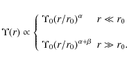
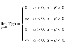
As an attempt to constrain
![]() ,
we can consider the following limits:
,
we can consider the following limits:
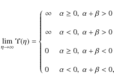
which show that models with
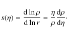
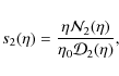
Further hints on the role of the different parameters at work may
be obtained considering the logarithmic slope of the global M/L ratio. It is:
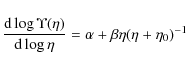
so that:
![\begin{displaymath}\frac{{\rm d}\log{\Upsilon(\eta)}}{{\rm d}\log{\eta}} \ge 0 \iff
\eta \ge \eta_{\rm c} = - [\alpha/(\alpha + \beta)] \eta_0.
\end{displaymath}](/articles/aa/full_html/2009/36/aa11090-08/img45.png)
Since we have decided to only consider models with
2.1 The luminosity density
The phenomenological ansatz for
![]() is just one side of the coin,
the other one being the choice of the luminosity profile. In principle,
this quantity may be directly reconstructed from the data by first
deconvolving the observed surface brightness with the PSF of the images and
then deprojecting it under an assumption for the intrinsic flattening.
Needless to say, such an idealized procedure is strongly affected by noise
and will call for a case - by - case study. Fortunately, ETGs are quite
regular in their photometric properties. Indeed, as well known
(Caon et al. 1993; Graham & Colless 1997; Prugniel & Simien 1997), their surface brightness is well described by the
Sersic profile (Sersic 1968):
is just one side of the coin,
the other one being the choice of the luminosity profile. In principle,
this quantity may be directly reconstructed from the data by first
deconvolving the observed surface brightness with the PSF of the images and
then deprojecting it under an assumption for the intrinsic flattening.
Needless to say, such an idealized procedure is strongly affected by noise
and will call for a case - by - case study. Fortunately, ETGs are quite
regular in their photometric properties. Indeed, as well known
(Caon et al. 1993; Graham & Colless 1997; Prugniel & Simien 1997), their surface brightness is well described by the
Sersic profile (Sersic 1968):
![\begin{displaymath}I(R) = I_{\rm e} \exp{\left \{ - b_n \left [ \left ( \frac{R}{R_{\rm eff}} \right
)^{1/n}
- 1 \right ] \right \}}
\end{displaymath}](/articles/aa/full_html/2009/36/aa11090-08/img49.png)
with R the cylindrical radius
where
The deprojection of the intensity profile in Eq. (8) is straightforward under the hypothesis of spherical symmetry, but, unfortunately, the result turns out to be a somewhat involved combinations of the unusual Meijer functions (Mazure & Capelato 2002). In order to not deal with these difficult to handle expression, we prefer to use the model proposed by Prugniel & Simien (1997, hereafter PS97) whose three dimensional luminosity density reads:
![\begin{displaymath}j(r) = j_0 \left ( \frac{r}{R_{\rm eff}} \right )^{-p_n} \exp...
... [ -b_n
\left (
\frac{r}{R_{\rm eff}} \right )^{1/n} \right ]}
\end{displaymath}](/articles/aa/full_html/2009/36/aa11090-08/img56.png)
with
![\begin{displaymath}j_0 = \frac{I_0 b_n^{n (1 - p_n)}}{2 R_{\rm eff}} \frac{\Gamma(2n)}{\Gamma[n (3
- p_n)]}\cdot
\end{displaymath}](/articles/aa/full_html/2009/36/aa11090-08/img57.png)
Here,
Because of the assumed spherical symmetry, the luminosity profile may simply be obtained as:
which, for the PS model, becomes:
![\begin{displaymath}L(r) = L_{\rm T} {\times} \frac{\gamma[n (3 - p_n), b_n \eta^{1/n})}{\Gamma[n (3
- p_n)]}
\end{displaymath}](/articles/aa/full_html/2009/36/aa11090-08/img62.png)
where the total luminosity
Note that the total luminosity is the same as the projected one for the corresponding Sersic profile as can be immediately check computing:
It is worth remembering the definitions of the different special functions entering Eqs. (9)-(13):
so that the following useful relations hold:
As a final remark, let us stress that the total mass of the stellar component
2.2 The total mass, density profile and DM fraction
Combining Eqs. (1) and (12), we trivially get for
the total mass profile:
![$\displaystyle \Upsilon_0 L_{\rm T} \left ( \frac{\eta}{\eta_0} \right )^{\alpha...
... \right )^{\beta} \frac{\gamma[n(3 - p_n), b_n
\eta^{1/n}]}{\Gamma[n(3 - p_n)]}$](/articles/aa/full_html/2009/36/aa11090-08/img72.png)
![$\displaystyle \Upsilon_{\rm eff}
L_{\rm T} \ \frac{\eta^{\alpha} (\eta + \eta_0...
...ma[n(3 - p_n), b_n \eta^{1/n}}
{(1 + \eta_0)^{\beta} \ \Gamma[n(3 - p_n)]}\cdot$](/articles/aa/full_html/2009/36/aa11090-08/img73.png)
Formally, M(r) diverges if
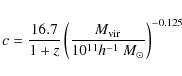
and, following Bryan & Norman (1998), we approximate the virial overdensity as:
where
The total mass is then the virial one obtained by setting
![\begin{displaymath}R_{\rm vir} = \left [ \frac{3 M_{\rm vir}}{4 \pi \Delta_c
\bar{\rho}_M(z)} \right ]^{1/3},
\end{displaymath}](/articles/aa/full_html/2009/36/aa11090-08/img81.png) |
(15) |
and solving with respect to
![\begin{displaymath}M_{\rm vir} = \Upsilon_{\rm eff} L_{\rm T} \ \times \
\frac{\...
..., b_n \eta^{1/n}]}{(1 + \eta_0)^{\beta} \ \Gamma[n(3 - p_n)]},
\end{displaymath}](/articles/aa/full_html/2009/36/aa11090-08/img83.png)
so that one can conveniently rewrite the mass profile as:
![$\displaystyle M(r) = M_{\rm vir}
\frac{(\eta/\eta_0)^{\alpha} (1 + \eta/\eta_0)...
... +
\eta_{\rm vir}/\eta_0)^{\beta} \gamma[n(3 - p_n), b_n \eta_{\rm vir}^{1/n}]}$](/articles/aa/full_html/2009/36/aa11090-08/img84.png)
which clearly shows that
![$\displaystyle \frac{{\rm d}\ln{M}}{{\rm d}\ln{\eta}} = \frac{\left ( b_n \eta^{...
...) + \beta \eta \right ]
\gamma[n(3 - p_n), b_n \eta^{1/n}]}{\eta + \eta_0}\cdot$](/articles/aa/full_html/2009/36/aa11090-08/img88.png) |
(17) |
It is instructive to first consider the case n = 4. We get:
so that only models with
Not surprisingly, this is the same constraint we have obtained when considering the logarithmic slope of the global M/L ratio
which is clearly an unphysical result. However, one can consider our ansätz for
Because of the assumed spherical symmetry, the mass density may be
straightforwardly derived as:
Using Eq. (16) and some lengthy algebra, we finally get:
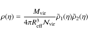
with:
![\begin{displaymath}{\cal{N}}_{\rm vir} = \left ( \frac{\eta_{\rm vir}}{\eta_0} \...
...a}
\gamma \left [n(3 - p_n), b_n
\eta_{\rm vir}^{1/n}\right ],
\end{displaymath}](/articles/aa/full_html/2009/36/aa11090-08/img96.png)
![$\displaystyle \tilde{\rho}_2 = \left ( 1 + \frac{\eta}{\eta_0} \right )
(b_n \e...
... ) \eta \right ]
\gamma[n(3 - p_n), b_n \eta^{1/n}] \ {\rm e}^{b_n \eta^{1/n}}.$](/articles/aa/full_html/2009/36/aa11090-08/img98.png)
It is worth stressing that Eq. (18) reduces to the stellar mass profile (10) setting
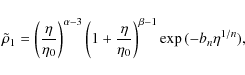
Some lengthy algebra finally gives:
having defined:
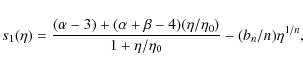
The density profile may be locally approximated as a power law with a running slope, i.e. we may write
so that we get the constraint
As a final cautionary remark, we stress that the logarithmic slope
![]() in Eq. (22) refers to the density law of the
effective model defined by our ansatz for the global M/L ratio.
As such,
in Eq. (22) refers to the density law of the
effective model defined by our ansatz for the global M/L ratio.
As such, ![]() is not the logarithmic slope of the (eventually
present) dark halo model. Actually, while in the outer regions the
stellar density may be neglected so that
is not the logarithmic slope of the (eventually
present) dark halo model. Actually, while in the outer regions the
stellar density may be neglected so that ![]() may be
identified with the
may be
identified with the
![]() ,
in the inner regions things
are more involved. In particular, an inner core of the effective
density profile, i.e.
,
in the inner regions things
are more involved. In particular, an inner core of the effective
density profile, i.e.
![]() ,
does not imply
that the corresponding dark halo model is a cored one.
,
does not imply
that the corresponding dark halo model is a cored one.
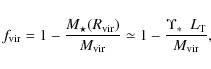
Finally, one of the main outcomes of our analysis is the spherical
DM content in the core of galaxies, typically within
![]() .
We define the spherical DM fraction within the radius r as
.
We define the spherical DM fraction within the radius r as
 |
(29) |
where
2.3 The surface mass density
A further quantity to be discussed is the surface mass density,
which we compute as:
having defined R = (x2 + y2)1/2 as usual. It is convenient to rewrite the above integral as:
with
with:
![$\displaystyle {\times} \exp{\left [ -b_n \left (
\frac{\xi}{\sin{\theta}} \right )^{1/n} \right ]} {\rm d}\theta,$](/articles/aa/full_html/2009/36/aa11090-08/img134.png)
![$\displaystyle \frac{\Upsilon_0 L_{\rm T}}{2 \pi R_{\rm eff}^2} \
\frac{\tilde{\Sigma}(\xi = 1)} {n \eta_0^{\alpha} \Gamma[n(3 -
p_n)]}$](/articles/aa/full_html/2009/36/aa11090-08/img137.png)
![$\displaystyle \frac{\Upsilon_{\rm eff} L_{\rm T}}{2 \pi
R_{\rm eff}^2} \ \frac{...
...beta} \tilde{\Sigma}(\xi = 1)}
{n (1 +
\eta_0)^{\beta} \Gamma[n(3 - p_n)]}\cdot$](/articles/aa/full_html/2009/36/aa11090-08/img138.png)
Equation (30) clearly shows the role of the different model parameters. Indeed, while
2.4 Projected mass and DM fraction
A quite interesting derived quantity, which will be useful when
contrasting models against observations, is the projected mass
within a circular aperture of radius R given by:
which, for our model, reduces to:
For the Prugniel-Simien model we are adopting for the luminosity component, the projected mass is given by:
![\begin{displaymath}M_{\rm proj}^{\rm PS}(\xi) = \mbox{$\Upsilon_{*}$ }\ L_{\rm T...
...ft [ 1 - \frac{\Gamma(2n, b_n
\xi^{1/n})}{\Gamma(2n)} \right ]
\end{displaymath}](/articles/aa/full_html/2009/36/aa11090-08/img148.png)
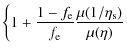
so that the projected DM mass fraction reads:

![$\displaystyle 1 - \frac{n \Gamma[n(3 - p_n)]}{\Upsilon_{\rm eff}/\mbox{$\Upsilon_{*}$ }}
\left ( \frac{1 + \eta_0}{\eta_0} \right )^{\beta}$](/articles/aa/full_html/2009/36/aa11090-08/img151.png)
It is worth noting that the projected mass fraction is typically higher than the spherical mass fraction
3 Dynamical and gravitational lensing properties
While photometric observations probe the light distribution (hence
giving constraints on the luminosity density), dynamical observables
(e.g., velocity dispersion) and gravitational lensing are excellent probes
of the mass profile. In the framework of our phenomenological scenario,
we can tell that dynamical and lensing observables make it possible to
constrain the global M/L ratio
![]() .
Therefore, it is
interesting to derive these main properties for our model.
.
Therefore, it is
interesting to derive these main properties for our model.
3.1 Velocity dispersion
A widely used probe to constrain the model parameters is
represented by the line of sight velocity dispersion luminosity
weighted within a circular aperture of radius
![]() .
This can
be easily evaluated as:
.
This can
be easily evaluated as:
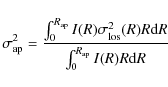
with
![$\displaystyle \sigma_{\rm ap}^2 = \frac{4 \pi G}{3 L_2(R_{\rm ap})} \left [
\in...
...m ap}}^{\infty}{(r^2 - R_{\rm ap}^2)^{3/2} j(r) M(r)
r^{-2} {\rm d}r} \right ],$](/articles/aa/full_html/2009/36/aa11090-08/img161.png)
with
the projected luminosity profile. For the model we are considering, after some algebra, we finally get:

![$\displaystyle \frac{G \Upsilon_{\rm eff}
L_{\rm T}}{R_{\rm eff}} \ \frac{b_n^{n...
...\Gamma[n(3
- p_n)]} \
\left ( \frac{\eta_0^\alpha}{1 + \eta_0} \right )^{\beta}$](/articles/aa/full_html/2009/36/aa11090-08/img165.png)

where we set
![$\displaystyle \int_{0}^{\infty}{\left (
\frac{\eta}{\eta_0} \right )^{\alpha} \...
...\{ 1 - \frac{\Gamma[n(3
- p_n), b_n \eta^{1/n}]}{\Gamma[n(3 - p_n)]} \right \}}$](/articles/aa/full_html/2009/36/aa11090-08/img171.png)
![$\displaystyle \int_{\xi_{\rm ap}}^{\infty}{\left (
\frac{\eta}{\eta_0} \right )...
...\{ 1 - \frac{\Gamma[n(3
- p_n), b_n \eta^{1/n}]}{\Gamma[n(3 - p_n)]} \right \}}$](/articles/aa/full_html/2009/36/aa11090-08/img174.png)
For given values of the model parameters, Eq. (38) allows us to predict the value of
3.2 Lensing observables
Gravitational lensing is a powerful tool to further constrain the space of parameters. After having determined the surface mass density in the previous section, here, we define the deflection angle, that allows a model independent estimate of projected mass at Einstein radius to be determined.
3.2.1 The deflection angle
A key role in the determination of the lensing properties of a given model is played by the deflection angle. For a spherically symmetric lens, this reads (Schneider et al. 1992):
where the critical surface density
with
where we have defined
![$\displaystyle 2 R_{\rm eff} \frac{\Upsilon_{\rm eff} L_{\rm T}}{2 \pi \Sigma_{\...
...\beta} \tilde{\alpha}(\xi = 1)}{n (1 + \eta_0)^{\beta} \Gamma[n(3 - p_n)]}\cdot$](/articles/aa/full_html/2009/36/aa11090-08/img190.png)
Looking at Eqs. (42) and (44), it is immediately clear that the Sersic index n and the model parameters
3.2.2 The Einstein angle
Should the source be a distant pointlike object (such as a
quasar), one may observe multiple images and then use their
positions to constrain the model parameters. On the other hand,
when the source is an extended object approximately aligned with
the lens along the line of sight, the formation of arcs takes
place. The angular radius of the circle individuated by these arcs
is the Einstein angle ![]() .
Referring the interested reader to
the literature for more details, we here only remember that the
Einstein angle may be determined by solving:
.
Referring the interested reader to
the literature for more details, we here only remember that the
Einstein angle may be determined by solving:
with
with
4 Testing the model global M/L ratio
Our proposed parametrization for
![]() was motivated by
the need to have a versatile expression able to mimic a large set
of galaxy models. Since we assume that the stellar component is
fixed and described by a PS density profile, mimicking a large set
of models is the same as mimicking the global M/L ratio predicted
by different dark halo models. Needless to say, such an ambitious
goal is difficult to reach so that we expect that Eq. (1) does a good job over a limited radial range. It is
therefore worth exploring how large is this range and how good and
versatile is our approximated parametrization.
was motivated by
the need to have a versatile expression able to mimic a large set
of galaxy models. Since we assume that the stellar component is
fixed and described by a PS density profile, mimicking a large set
of models is the same as mimicking the global M/L ratio predicted
by different dark halo models. Needless to say, such an ambitious
goal is difficult to reach so that we expect that Eq. (1) does a good job over a limited radial range. It is
therefore worth exploring how large is this range and how good and
versatile is our approximated parametrization.
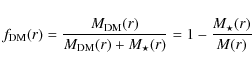
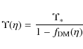
To this aim, it is convenient to resort to the following general
expression for the mass profile of the dark halo:
with
![\begin{displaymath}f_{\rm DM}(\eta) = \left [ 1 + \frac{M_{\star}(\eta)}{M_{\rm DM}(\eta)}
\right ]^{-1}\cdot
\end{displaymath}](/articles/aa/full_html/2009/36/aa11090-08/img204.png)
Normalizing with respect to
![$\displaystyle \left . \frac{1 + \Gamma[n(3 - p_n), b_n \eta^{1/n}]/\Gamma[n(3 - p_n)]}
{1 + \Gamma[n(3 - p_n),b_n]/\Gamma[n(3 - p_n)]} \right \}^{-1}$](/articles/aa/full_html/2009/36/aa11090-08/img209.png)
which may then be related to the global M/L ratio as:
having assumed a constant stellar M/L ratio. Eq. (47) makes it possible to compute the DM mass fraction and hence the global M/L ratio through Eq. (48) provided that an expression for
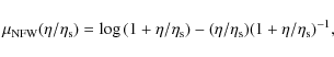
To test the validity of our phenomenological ansatz, we start
considering the most popular galaxy profiles, i.e. NFW
(Navarro
et al. 1996, 1997), the Einasto
(Einasto 1965; Einasto & Haud 1989; Navarro et al. 2004; Cardone et al. 2005), the
nonsingular isothermal sphere and the Burkert (1995) models. Using
the formalism introduced above, the cumulative mass profile for
each case is assigned by the following expressions:
![\begin{displaymath}\mu_{\rm Ein}(\eta) = 1 - \frac{\Gamma[2n_{\rm DM}, {\rm d}_n
(\eta/\eta_{\rm s})^{1/n_{\rm DM}}]}{\Gamma(2n_{\rm DM})},
\end{displaymath}](/articles/aa/full_html/2009/36/aa11090-08/img213.png)
![\begin{displaymath}\mu_{\rm Bur}(\eta) = \frac{\ln{[1 + (\eta/\eta_{\rm s})^2]}}...
...[1 + (\eta/\eta_{\rm s})]} - \arctan{(\eta/\eta_{\rm s})}}{2}.
\end{displaymath}](/articles/aa/full_html/2009/36/aa11090-08/img215.png)
We parameterize NFW profile assigning first the virial mass
also taking care of the large scatter. It is worth noting that, by virtue of the
Once the halo parameters have been set, we add a stellar component
fixing the photometric parameters
![]() ,
the stellar M/L ratio
,
the stellar M/L ratio
![]() and the redshift z so that they are equal to those of a
randomly chosen lens. We then fit Eq. (1) to the
resulting
and the redshift z so that they are equal to those of a
randomly chosen lens. We then fit Eq. (1) to the
resulting
![]() profile and repeat this exercise for
1000 random realizations of each halo model. The instructive results of
this investigation are schematically summarized below.
profile and repeat this exercise for
1000 random realizations of each halo model. The instructive results of
this investigation are schematically summarized below.
- -
- Equation (1) fits the
 of the
tested models with a very good precision and over a large radial
range, namely
of the
tested models with a very good precision and over a large radial
range, namely
 .
Denoting with
.
Denoting with
 our
proposed function and defining
our
proposed function and defining
 ,
we get that the maximal deviation is lower than
,
we get that the maximal deviation is lower than  (depending on the model).
In particular, for NFW is
(depending on the model).
In particular, for NFW is
 and
and
 .
The Einasto model is fitted with
.
The Einasto model is fitted with
 ,
while the worst performances are obtained
for the Burkert one for which we, however, find a still
satisfactory
,
while the worst performances are obtained
for the Burkert one for which we, however, find a still
satisfactory
 .
.
- -
- The fitted model parameters
 depend on the halo parameters so that a general rule cannot be
given. However, we note that quite small and negative values of
depend on the halo parameters so that a general rule cannot be
given. However, we note that quite small and negative values of
 are clearly preferred for the NFW+PS input model. This is
somewhat surprising since this would give rise to models with an
inner asymptotic slope of the global density
are clearly preferred for the NFW+PS input model. This is
somewhat surprising since this would give rise to models with an
inner asymptotic slope of the global density
 ,
contrary to popular models having
,
contrary to popular models having
 .
However,
as stated above, in the very inner regions our model does not fit
anymore the NFW + PS one so that the results on s0 can not be
trusted upon. For this same reason, we do not care about obtaining
still more negative values of .
Indeed, for the other
models,
.
However,
as stated above, in the very inner regions our model does not fit
anymore the NFW + PS one so that the results on s0 can not be
trusted upon. For this same reason, we do not care about obtaining
still more negative values of .
Indeed, for the other
models,
 cases are still clearly preferred. As a
conservative estimate, we therefore conclude that, in order our
parametrization fits well different dark halo models, one must
have negative ,
with values as low as
cases are still clearly preferred. As a
conservative estimate, we therefore conclude that, in order our
parametrization fits well different dark halo models, one must
have negative ,
with values as low as
 .
.
- -
- The asymptotic outer slope
 typically
takes values of order 1-2, even if one cannot exclude
values as high as
typically
takes values of order 1-2, even if one cannot exclude
values as high as
 .
For example, if
considering the NFW + PS,
is strongly peaked on
the
.
For example, if
considering the NFW + PS,
is strongly peaked on
the  2, and the distributions is markedly asymmetric with
long tails towards larger values. In contrast,
has a similar distribution, but shifted to the smaller
2, and the distributions is markedly asymmetric with
long tails towards larger values. In contrast,
has a similar distribution, but shifted to the smaller
 peak, for cored models. As a general rule, however,
 never occurs in agreement with our above discussion
showing that such models have an unphysically decreasing mass
profile.
never occurs in agreement with our above discussion
showing that such models have an unphysically decreasing mass
profile.
- -
- The scaling quantities
 and
and
 are in the range
 and
and
 .
In particular, if considering the NFW + PS,
and
are strongly peaked on
.
In particular, if considering the NFW + PS,
and
are strongly peaked on
 and 0.5 respectively. Similar values are obtained for the
other dark halo models considered, a result which is not fully unexpected.
Indeed,
and 0.5 respectively. Similar values are obtained for the
other dark halo models considered, a result which is not fully unexpected.
Indeed,
 and
are mostly
related respectively to the virial mass
and
are mostly
related respectively to the virial mass
 and DM mass fration
  and to the scaled virial radii
 .
Since these quantities take
similar values for all models, we indeed expect to find a not too large scatter
among different models which is indeed what we find.
.
Since these quantities take
similar values for all models, we indeed expect to find a not too large scatter
among different models which is indeed what we find.
- -
- Changing the
 relation or its scatter does
not alter the result on the validity of our approximation for NFW + PS profile,
i.e.
relation or its scatter does
not alter the result on the validity of our approximation for NFW + PS profile,
i.e.
 and
and
 span the same range as above for
 covering the same radial range. However, the distribution
of the fitted parameters may change significantly. In particular,
higher values of
may be obtained although negative
are still preferred
covering the same radial range. However, the distribution
of the fitted parameters may change significantly. In particular,
higher values of
may be obtained although negative
are still preferred![[*]](/icons/foot_motif.png) . Considering that similar values for can be obtained by fitting
to models other than NFW, we
argue that it is not possible to resort to
to discriminate between,
e.g., the NFW and the Einasto models, or cusped and cored profiles, unless
one has a precise determination of the
relation.
. Considering that similar values for can be obtained by fitting
to models other than NFW, we
argue that it is not possible to resort to
to discriminate between,
e.g., the NFW and the Einasto models, or cusped and cored profiles, unless
one has a precise determination of the
relation.
5 Model vs observations
The phenomenological ansatz for
![]() we are proposing is
characterized by four parameters, namely the two asymptotic
slopes
we are proposing is
characterized by four parameters, namely the two asymptotic
slopes![]() , the logarithm of the scaling length
, the logarithm of the scaling length
![]() and the global M/L ratio at the effective radius
and the global M/L ratio at the effective radius
![]() .
To these four quantities, we have to add the
stellar M/L ratio
.
To these four quantities, we have to add the
stellar M/L ratio
![]() thus leading to five the number of
unknown quantities to be constrained. Needless to say, tackling
such an issue is a quite daunting task. A possible way out could
be contrasting the model with kinematic observations, such as the
velocity dispersion profile. To this aim, the data should cover a
radial range wide enough to sample with sufficient detail both the
inner and the outer regions in order to constrain the two
asymptotic slopes. Moreover, the measurement errors and the
sampling should be extremely good to overcome the problem of
parameters degeneracies in a five dimensional space. All these
observational requirements are quite demanding so as to be
satisfied only by a handful number of nearby galaxies. Actually,
we are interested here in lens galaxies with typical redshifts of
order 0.1 - 0.5 so that measuring their velocity dispersion
profile with the above precision and sampling is an unrealistic
task. Nevertheless, for each galaxy, we still have two observable
quantities that can be used, namely the Einstein angle
thus leading to five the number of
unknown quantities to be constrained. Needless to say, tackling
such an issue is a quite daunting task. A possible way out could
be contrasting the model with kinematic observations, such as the
velocity dispersion profile. To this aim, the data should cover a
radial range wide enough to sample with sufficient detail both the
inner and the outer regions in order to constrain the two
asymptotic slopes. Moreover, the measurement errors and the
sampling should be extremely good to overcome the problem of
parameters degeneracies in a five dimensional space. All these
observational requirements are quite demanding so as to be
satisfied only by a handful number of nearby galaxies. Actually,
we are interested here in lens galaxies with typical redshifts of
order 0.1 - 0.5 so that measuring their velocity dispersion
profile with the above precision and sampling is an unrealistic
task. Nevertheless, for each galaxy, we still have two observable
quantities that can be used, namely the Einstein angle ![]() and
and
![]() ,
the line of sight velocity dispersion luminosity
weighted in a circular aperture of radius
,
the line of sight velocity dispersion luminosity
weighted in a circular aperture of radius
![]() .
Needless to
say, it is impossible to constraint a five dimensional parameter
space with only two datapoints so that a case-by-case
analysis is not possible. In order to overcome such a problem, we
have therefore to reduce the number of unknowns and increase the
number of observed datapoints. To this aim, we therefore first get
an estimate of the stellar M/L ratio
.
Needless to
say, it is impossible to constraint a five dimensional parameter
space with only two datapoints so that a case-by-case
analysis is not possible. In order to overcome such a problem, we
have therefore to reduce the number of unknowns and increase the
number of observed datapoints. To this aim, we therefore first get
an estimate of the stellar M/L ratio
![]() .
.
5.1 Stellar M/L
We start assembling a library of synthetic stellar population
models obtained through the Galaxev code (Bruzual & Charlot 2003)
varying the age of the population, its metallicity and time lag of
the exponential star formation rate and assuming a Chabrier (2001)
initial mass function (IMF). Then, we use the tabulated
(u, g, r,
i, z) apparent magnitudes (corrected for extinction) of each lens
to fit the above library of spectra (suitably redshifted to lens
redshift) to the colours, thus getting the estimates reported in
Table 1. Note that these values may be easily scaled to a Salpeter
(1955) or Kroupa (2001) IMF by multiplying by 1.8 or 1.125respectively so that we can explore other IMF
choices![]() . In order to get the
. In order to get the
![]() uncertainties, we
use a Monte Carlo-like procedure generating a set of colours
from a Gaussian distribution centred on each mean colour and
standard deviation equal to the colour uncertainty. Fitting the
colours thus obtained to the synthetic spectra for each
realization, we generate a distribution of fitted parameters. The
median and median scatter of such a distribution is finally taken
as an estimate of
uncertainties, we
use a Monte Carlo-like procedure generating a set of colours
from a Gaussian distribution centred on each mean colour and
standard deviation equal to the colour uncertainty. Fitting the
colours thus obtained to the synthetic spectra for each
realization, we generate a distribution of fitted parameters. The
median and median scatter of such a distribution is finally taken
as an estimate of
![]() and its uncertainty (see Tortora et al.
2009, for further details).
and its uncertainty (see Tortora et al.
2009, for further details).
5.2 Resorting to universal parameters
Having reduced by one the number of parameters, we now look for a
way to increase the number of constraints. To this aim, we could
stack all the lenses in a single sample. However, while one can
reasonably argue that the same functional expression for
![]() describes the global M/L ratio of all the lenses,
its characterizing parameters are likely to change on a
case-by-case basis. Indeed, even if we assume that the DM
halo has a universal profile, the details of the baryonic assembly
may lead to different model parameters. In order to partially
alleviate this problem, we therefore reparametrize
describes the global M/L ratio of all the lenses,
its characterizing parameters are likely to change on a
case-by-case basis. Indeed, even if we assume that the DM
halo has a universal profile, the details of the baryonic assembly
may lead to different model parameters. In order to partially
alleviate this problem, we therefore reparametrize
![]() in Eq. (1) in terms of quantities that are likely
to be (at least, to first order) universal.
in Eq. (1) in terms of quantities that are likely
to be (at least, to first order) universal.
Table 1: Photometric and lensing observables and estimated stellar M/L ratio for the 21 SLACS lenses.
To this aim, it is worth remembering that previous works on
fitting galaxy models to the lenses using the constraints from the
Einstein ring and the velocity dispersion concordantly suggest
that the total mass profile at
![]() is well approximated by
a singular isothermal sphere (see, e.g., Treu & Koopmans 2004, and refs.
therein). Actually, rather than constraining the global mass
profile, such an analysis essentially probe the shape of the
density profile only at the Einstein radius so that one can argue
that the logarithmic slope of the density profile at
is well approximated by
a singular isothermal sphere (see, e.g., Treu & Koopmans 2004, and refs.
therein). Actually, rather than constraining the global mass
profile, such an analysis essentially probe the shape of the
density profile only at the Einstein radius so that one can argue
that the logarithmic slope of the density profile at
![]() is the
same for all lenses. Motivated by these previous literature
results, we therefore assume that
is the
same for all lenses. Motivated by these previous literature
results, we therefore assume that
![]() is the
same for all lenses and use this quantity as model parameter
instead of
is the
same for all lenses and use this quantity as model parameter
instead of
![]() .
To this aim, for given values of
.
To this aim, for given values of
![]() ,
we numerically solve:
,
we numerically solve:
with respect to
and setting
![\begin{displaymath}\Upsilon_{\rm eff} = \frac{M_{\rm vir}}{\eta_0^{\alpha} L_{\r...
...mma[n(3 - p_n)]}{\gamma[n(3 - p_n), b_n \eta_{\rm vir}^{1/n}]}
\end{displaymath}](/articles/aa/full_html/2009/36/aa11090-08/img308.png)
with
Unfortunately, we are unable to find other lens related parameters
that can be considered universal so that we will hereafter
parameterize our
![]() ansatz with the slope parameters
ansatz with the slope parameters
![]() and
and
![]() ,
the logarithmic slope at the scaled
Eintein radius
,
the logarithmic slope at the scaled
Eintein radius
![]() ,
and the mass ratio at the
virial radius
,
and the mass ratio at the
virial radius
![]() assuming that these
are universal quantities. In order to explore the impact of this
theoretical hypothesis, we will fit our model to the full lens
sample and to four subsamples containing respectively five, six,
six, four lenses binned according to the absolute V magnitude
MV. Comparing the constraints on the model parameters obtained
by the different fits makes it possible to look for an eventual
dependence on the lens luminosity thus giving an a posteriori
check of our a priori assumption.
assuming that these
are universal quantities. In order to explore the impact of this
theoretical hypothesis, we will fit our model to the full lens
sample and to four subsamples containing respectively five, six,
six, four lenses binned according to the absolute V magnitude
MV. Comparing the constraints on the model parameters obtained
by the different fits makes it possible to look for an eventual
dependence on the lens luminosity thus giving an a posteriori
check of our a priori assumption.
5.3 Statistical analysis
As shown by Eq. (45), a measurement of
![]() may be
considered as a measurement of the deflection angle
may be
considered as a measurement of the deflection angle
![]() so that stacking together many galaxies with different values of
so that stacking together many galaxies with different values of
![]() makes it possible to reconstruct the deflection angle profile. Similarly, since
makes it possible to reconstruct the deflection angle profile. Similarly, since
![]() is weighted within an aperture of fixed angular
radius
is weighted within an aperture of fixed angular
radius
![]() but different normalized radii
but different normalized radii
![]() ,
this is the same as tracing the luminosity weighted line of
sight dispersion profile. The agreement within the model and the
data may then be optimized by maximizing the likelihood
function:
,
this is the same as tracing the luminosity weighted line of
sight dispersion profile. The agreement within the model and the
data may then be optimized by maximizing the likelihood
function:
![\begin{displaymath}{\cal{L}}({\bf p}) \propto \exp{\left [- \frac{\chi^2_{\rm lens}({\bf p}) +
\chi^2_{\rm dyn}({\bf p})}{2} \right ]}
\end{displaymath}](/articles/aa/full_html/2009/36/aa11090-08/img312.png)
with
The Markov Chains may also be used to extract constraints on some
interesting derived quantities. To this aim, let us consider a
generic function
![]() .
Evaluating y along the
chains, we can build up the histogram of its values and then use
the median and quantiles of this latter to infer the Bayesian
confidence levels on y. Such a procedure will be used for the
scaling model parameters
.
Evaluating y along the
chains, we can build up the histogram of its values and then use
the median and quantiles of this latter to infer the Bayesian
confidence levels on y. Such a procedure will be used for the
scaling model parameters
![]() and
and
![]() and
for the projected and spherical DM mass fractions for each lens in
the sample.
and
for the projected and spherical DM mass fractions for each lens in
the sample.
5.3.1 The lensing merit function
Dealing with the Einstein angle as a constraint is not
straightforward. Indeed, for a given set of model parameters,
![]() should be find solving Eq. (45) so that a lot
of computing time should be spent to explore the four dimensional
parameter space. Moreover, the photometric parameters
should be find solving Eq. (45) so that a lot
of computing time should be spent to explore the four dimensional
parameter space. Moreover, the photometric parameters
![]() entering Eq. (45) are affected by their own
uncertainties so that one should solve this relation many times
by, for instance, bootstrapping the values of these quantities and
looking for the corresponding uncertainty induced on the predicted
entering Eq. (45) are affected by their own
uncertainties so that one should solve this relation many times
by, for instance, bootstrapping the values of these quantities and
looking for the corresponding uncertainty induced on the predicted
![]() .
Fortunately, we can skip all these complications by
resorting to the projected mass within the Einstein radius whose
theoretical and observed values may be estimated from
Eqs. (33) and (46).
.
Fortunately, we can skip all these complications by
resorting to the projected mass within the Einstein radius whose
theoretical and observed values may be estimated from
Eqs. (33) and (46).
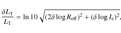
Because of the measurement errors on ![]() and
and
![]() and the
uncertainty on
and the
uncertainty on
![]() coming from the one on
coming from the one on
![]() ,
the
predicted
,
the
predicted
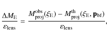
![]() is affected by an uncertainty
which we naively quantity using error propagation as:
is affected by an uncertainty
which we naively quantity using error propagation as:
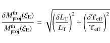
with:
note that we have here neglected the contribution of the error on
We finally define the lensing merit function as:
![\begin{displaymath}\chi^2_{\rm lens}({\bf p}) = \sum_{i = 1}^{{\cal{N}}}{\left [...
...xi_{\rm E}, {\bf p})}
{\varepsilon_{{\rm lens},i}} \right ]^2}
\end{displaymath}](/articles/aa/full_html/2009/36/aa11090-08/img330.png)
where the total uncertainty
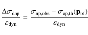
5.3.2 The dynamics figure of merit
Denoting with
![]() the observed value, we define the
following figure of merit for the dynamical data:
the observed value, we define the
following figure of merit for the dynamical data:
![\begin{displaymath}\chi^2_{{\rm dyn}}({\bf p}) = \sum_{i = 1}^{{\cal{N}}} {\left...
...p,th}}^{(i)}({\bf p})}
{\varepsilon_{{\rm dyn},i}} \right ]^2}
\end{displaymath}](/articles/aa/full_html/2009/36/aa11090-08/img334.png)
where
5.4 The data
The sums in Eqs. (53) and (54)
run over the ![]() objects in the sample. It is therefore
vital to specify what this sample is made of. We consider here the
21 lens ETGs reported in Gavazzi et al. (2007) whose main properties
are summarized in Table 1 where columns are as follows: 1.
name (without the prefix SDSS); 2. lens redshift; 3. source
redshift; 4. absolute V magnitude (incremented by
objects in the sample. It is therefore
vital to specify what this sample is made of. We consider here the
21 lens ETGs reported in Gavazzi et al. (2007) whose main properties
are summarized in Table 1 where columns are as follows: 1.
name (without the prefix SDSS); 2. lens redshift; 3. source
redshift; 4. absolute V magnitude (incremented by ![]() );
5. effective radius (in arcsec); 6. Einstein radius (in
arcsec); 7. aperture velocity dispersion (in km s-1); 8. ratio
between the aperture and the effective radii; 9. estimated V-band
stellar M/L ratio with its error. Note that we do not have colours
for lens J223840.2+075456 so that
);
5. effective radius (in arcsec); 6. Einstein radius (in
arcsec); 7. aperture velocity dispersion (in km s-1); 8. ratio
between the aperture and the effective radii; 9. estimated V-band
stellar M/L ratio with its error. Note that we do not have colours
for lens J223840.2+075456 so that
![]() cannot be evaluated and
this object will be excluded by the analysis. These lenses have been
observed in the framework of the SLACS survey which aims at
confirming through ACS imaging candidate lenses spectroscopically
identified within the SDSS catalog (see Bolton et al. 2004, 2006, 2008,
for further details). The SDSS velocity dispersions have been
measured within a circular aperture of fixed radius
cannot be evaluated and
this object will be excluded by the analysis. These lenses have been
observed in the framework of the SLACS survey which aims at
confirming through ACS imaging candidate lenses spectroscopically
identified within the SDSS catalog (see Bolton et al. 2004, 2006, 2008,
for further details). The SDSS velocity dispersions have been
measured within a circular aperture of fixed radius
![]() and spans the range
and spans the range
![]() with a mean square velocity
with a mean square velocity
![]() .
The lens galaxies have a
mean redshift
.
The lens galaxies have a
mean redshift
![]() ,
but it is worth
noting that the redshift range covered (
,
but it is worth
noting that the redshift range covered (
![]() )
probes almost one order of magnitude (even if quite sparsely). The
measured surface brightness has been fitted by a de Vaucouleurs
(1948) model so that n will be fixed to 4 in the following.
Typical uncertainties on
)
probes almost one order of magnitude (even if quite sparsely). The
measured surface brightness has been fitted by a de Vaucouleurs
(1948) model so that n will be fixed to 4 in the following.
Typical uncertainties on
![]() and
and ![]() are quite small so
that, following Bolton et al. (2008), we will set
are quite small so
that, following Bolton et al. (2008), we will set
![]() for all
galaxies in the sample. Gavazzi et al. (2007) provides also
absolute V band magnitude corrected for filter transformation
and Galactic extinction and K and evolution corrected to a
common redshift z = 0.2. When fitting Einstein radius and
velocity dispersions, however, we need the luminosity at the lens
redshift. This can be easily estimated as (Gavazzi et al. 2007):
for all
galaxies in the sample. Gavazzi et al. (2007) provides also
absolute V band magnitude corrected for filter transformation
and Galactic extinction and K and evolution corrected to a
common redshift z = 0.2. When fitting Einstein radius and
velocity dispersions, however, we need the luminosity at the lens
redshift. This can be easily estimated as (Gavazzi et al. 2007):
with:
having set
with the effective surface brightness given by:
While
6 Results
The sample of 21 SLACS lenses represents the input dataset needed to
constrain the four model parameters
![]() through the Bayesian likelihood analysis described above.
As a first test, motivated by the above discussion, we fit the model to the
full sample without any binning in luminosity thus giving us a quite
large set of constraints (namely,
through the Bayesian likelihood analysis described above.
As a first test, motivated by the above discussion, we fit the model to the
full sample without any binning in luminosity thus giving us a quite
large set of constraints (namely,
![]() observable quantities vs. 4
parameters). Nevertheless, some care is needed when examining the results
of the Markov Chain analysis.
observable quantities vs. 4
parameters). Nevertheless, some care is needed when examining the results
of the Markov Chain analysis.
In order the results to be reliable, one should carefully check
that the chains have reached convergence, that is to say that the
chains have fully explored the regions of high likelihood. Should
this be the case, one should see the points of the chains for each
single parameter oscillate around an average value or, put another
way, the histograms of the parameters be single peaked
(eventually, with a Gaussian shape). In order to test the
convergence of the chains we resort to the test described in
Dunkley et al. (2005, see also Dunkley et al. 2009) which is based on the
analysis of the chain power spectra. Before checking for
convegence, however, we first cut out the initial ![]() of the
chain in order to avoid the burn in period. Moreover, to reduce
spurious correlations among parameters induced by the nature of
the Markov Chain process, we thin the chain by taking 1 point each 25.
We find that the convergence test is well passed for a chain
containing 105 points which reduces to 2801 after the burn in
cut and the thinning. Such a large sample is more than sufficient
to sample the four dimensional parameter space. Note that we have
also tried to change the burn in cut and thinning thus checking
that the results are unaffected by these (somewhat arbitrary)
choices.
of the
chain in order to avoid the burn in period. Moreover, to reduce
spurious correlations among parameters induced by the nature of
the Markov Chain process, we thin the chain by taking 1 point each 25.
We find that the convergence test is well passed for a chain
containing 105 points which reduces to 2801 after the burn in
cut and the thinning. Such a large sample is more than sufficient
to sample the four dimensional parameter space. Note that we have
also tried to change the burn in cut and thinning thus checking
that the results are unaffected by these (somewhat arbitrary)
choices.
Table 2: Results for the fit to the full lens sample.
Table 3: Results for the fit to the binned lenses.
6.1 Constraints on the model parameters
The results obtained fitting our model to the full SLACS sample are
summarized in Table 2 which reports, for each parameter, mean and median
values and 68 and ![]() confidence limits. First, we note that the
best fit model parameters turns out to be:
confidence limits. First, we note that the
best fit model parameters turns out to be:
giving
with
The low values of
Having established the validity of our model, let us now discuss
the constraints on its parameters. As a first lesson, we note that
models with
![]() are definitely excluded contrary to the
discussion in Sect. 2 where we have shown that negative
are definitely excluded contrary to the
discussion in Sect. 2 where we have shown that negative ![]() values lead to a global M/L ratio diverging for
values lead to a global M/L ratio diverging for
![]() .
However, such an unphysical behaviour is actually never
approached since, as we have seen in Sect. 5, our
phenomenological ansatz do not fit realistic models for
.
However, such an unphysical behaviour is actually never
approached since, as we have seen in Sect. 5, our
phenomenological ansatz do not fit realistic models for
![]() so that one has not to trust its extrapolation in the very
inner regions. On the other hand, the analysis in Sect. 5 have
shown that models with
so that one has not to trust its extrapolation in the very
inner regions. On the other hand, the analysis in Sect. 5 have
shown that models with
![]() are needed to fit the global
M/L ratios of different dark halo models. It is therefore
reassuring that the likelihood analysis indeed prefer this kind of
models thus leading further support to our phenomenological
approach. As a further remark, we also note that the values of
are needed to fit the global
M/L ratios of different dark halo models. It is therefore
reassuring that the likelihood analysis indeed prefer this kind of
models thus leading further support to our phenomenological
approach. As a further remark, we also note that the values of
![]() and
and
![]() are typical of cored dark halo
density profiles (such as the NIS and Burkert models). However,
the very small
are typical of cored dark halo
density profiles (such as the NIS and Burkert models). However,
the very small ![]() values obtained when considering the NFW
model are also partly due to the adopted mass-concentration
relation so that it is likely that changing the
values obtained when considering the NFW
model are also partly due to the adopted mass-concentration
relation so that it is likely that changing the
![]() relation may lead to larger and still negative
relation may lead to larger and still negative ![]() values.
Exploring this issue is outside our aims here, but we argue that
cored profiles are preferred on the basis of our phenomenological
approach.
values.
Exploring this issue is outside our aims here, but we argue that
cored profiles are preferred on the basis of our phenomenological
approach.
Table 4: Marginalized constraints on the model parameters for different bins.
A further success of our model is represented by the constraints
on ![]() ,
i.e. the logarithmic slope of the total density profile
at the scaled Einstein radius, i.e.
,
i.e. the logarithmic slope of the total density profile
at the scaled Einstein radius, i.e.
![]() .
Previous analysis in
literature have typically fitted the observed Einstein radius and
velocity dispersion using a parameterized density profile. For
instance, Koopmans & Treu (2003a,b) have fitted the data on
0047-281 and B1608+656 assuming
.
Previous analysis in
literature have typically fitted the observed Einstein radius and
velocity dispersion using a parameterized density profile. For
instance, Koopmans & Treu (2003a,b) have fitted the data on
0047-281 and B1608+656 assuming
![]() and
finding
and
finding
![]() and
and
![]() ,
respectively. Using the same methodology, but averaging
over a sample of 15 SLACS lenses, Koopmans et al. (2006) have found again
,
respectively. Using the same methodology, but averaging
over a sample of 15 SLACS lenses, Koopmans et al. (2006) have found again
![]() .
As yet said before and also
stressed by the same authors, these may be
considered as constraints on the logarithmic slope at the Einstein
radius since this is the range mainly probed by the data. It is
therefore reassuring that, using a similar data analysis but a
radically different parametrization, we get compatible constraints
on
.
As yet said before and also
stressed by the same authors, these may be
considered as constraints on the logarithmic slope at the Einstein
radius since this is the range mainly probed by the data. It is
therefore reassuring that, using a similar data analysis but a
radically different parametrization, we get compatible constraints
on ![]() thus strengthening our results.
thus strengthening our results.
Finally, we consider the
![]() parameter. It is easy to
transform the constraints on this quantity into one on the DM mass
fraction at the virial radius thus getting:
parameter. It is easy to
transform the constraints on this quantity into one on the DM mass
fraction at the virial radius thus getting:
Using
![\begin{figure}
\par\mbox{\subfigure{\includegraphics[width=8.29cm]{11090f1a.eps}...
...mskip}
\subfigure{\includegraphics[width=8.2cm]{11090f1d.eps} }}
\end{figure}](/articles/aa/full_html/2009/36/aa11090-08/img409.png) |
Figure 1:
Variation of the model parameters
with the median |
| Open with DEXTER | |
6.2 Binning the lenses
A simple analysis of the best fit residual to the full sample
shows that there is actually no correlation with either the lens
redshift, the total luminosity and stellar mass. Such a result may
argue in favour of our assumption about the universality of the
parameters
![]() .
However,
this can also be a consequence of an erroneous estimation of the
errors or of insufficient statistics. To further
explore this issue, we therefore divide the lenses in four almost
equally populated bins (denoted as B1, B2, B3, B4) according to
their absolute V magnitude and run our MCMC algorithm using
chains with
.
However,
this can also be a consequence of an erroneous estimation of the
errors or of insufficient statistics. To further
explore this issue, we therefore divide the lenses in four almost
equally populated bins (denoted as B1, B2, B3, B4) according to
their absolute V magnitude and run our MCMC algorithm using
chains with
![]() points reducing to 5601 after burn
in cut and thinning. Note that, because we use now a smaller
number of constraints (namely, 6 - 8 vs. 38), we have to run
longer chains in order to achieve the same convergence as with the
full sample. We summarise in Table 3 the best fit values
and statistics of residuals for the fits to the binned samples, reporting
in the second column the median value and the full range of MV in each bin,
while the two numbers in columns 4 and 5 refer to the mean and rms values of
the lensing and dynamics residuals, respectively. Table 4 reports the constraints
on the model parameters after marginalization using the notation
points reducing to 5601 after burn
in cut and thinning. Note that, because we use now a smaller
number of constraints (namely, 6 - 8 vs. 38), we have to run
longer chains in order to achieve the same convergence as with the
full sample. We summarise in Table 3 the best fit values
and statistics of residuals for the fits to the binned samples, reporting
in the second column the median value and the full range of MV in each bin,
while the two numbers in columns 4 and 5 refer to the mean and rms values of
the lensing and dynamics residuals, respectively. Table 4 reports the constraints
on the model parameters after marginalization using the notation
![]() to mean that x is the median value,
while
to mean that x is the median value,
while ![]() and
and ![]() CL read
(x - y1, x + z1) and
(x - y2, x + z2),
respectively. These results allow us to make some interesting considerations.
CL read
(x - y1, x + z1) and
(x - y2, x + z2),
respectively. These results allow us to make some interesting considerations.
As a first remark, we note that the fit is still successful as
witnessed by both the low normalized residuals and reduced
![]() values
values![]() . Actually, one could wonder why the reduced
. Actually, one could wonder why the reduced
![]() values for bin B1 and B4 are smaller than unity thus
arguing for a possible overestimate of the errors. While this is
possible since our estimate is based on a naive propagation not
taking into account correlations among the uncertainties on
photometric quantities, we nevertheless note that the
values for bin B1 and B4 are smaller than unity thus
arguing for a possible overestimate of the errors. While this is
possible since our estimate is based on a naive propagation not
taking into account correlations among the uncertainties on
photometric quantities, we nevertheless note that the
![]() values for bins B2 and B3 do not present such a
problem. Notwithstanding the solution of this ambiguity, we
however stress that the constraints on the model parameters are
not biased.
values for bins B2 and B3 do not present such a
problem. Notwithstanding the solution of this ambiguity, we
however stress that the constraints on the model parameters are
not biased.
It is interesting to compare the results on the marginalized model
parameters with the corresponding ones for the full sample. To
this aim, we look at Fig. 1 where we have plotted
the median and ![]() CL estimate of each parameter as a function
of the median
CL estimate of each parameter as a function
of the median ![]() of the bin and overplotted the results
from the fit to the full sample. As it is clear, it is not
possible to infer any statistically reliable trend for
of the bin and overplotted the results
from the fit to the full sample. As it is clear, it is not
possible to infer any statistically reliable trend for ![]() which is indeed constant within the errors and compatible with the
result from the fit to all lenses. A similar discussion may also
be done for
which is indeed constant within the errors and compatible with the
result from the fit to all lenses. A similar discussion may also
be done for
![]() ,
,
![]() and
and ![]() ,
which due to
large uncertainties cannot allow to determine strong trends with
luminosity. However, these figures seem to suggest interesting
trends as a function of
,
which due to
large uncertainties cannot allow to determine strong trends with
luminosity. However, these figures seem to suggest interesting
trends as a function of ![]() ,
which we will better explore
in a future paper enlarging the sample. Our results give
issues about a dependence of the parameters above on luminosity
and stellar mass, with brighter galaxies having on average higher
values for
,
which we will better explore
in a future paper enlarging the sample. Our results give
issues about a dependence of the parameters above on luminosity
and stellar mass, with brighter galaxies having on average higher
values for
![]() and
and
![]() and a profile more
similar to the isothermal sphere. Finally, an increase of
and a profile more
similar to the isothermal sphere. Finally, an increase of
![]() with luminosity and stellar mass implies that the star
formation efficiency
with luminosity and stellar mass implies that the star
formation efficiency
![]() decreases with these
quantities. Indeed, this is consistent with the observational and
theoretical studies (Benson et al. 2000; Napolitano et al. 2005; Conroy & Wechsler 2008; Tortora
et al. 2009a; Napolitano et al. 2009) showing that more massive
galaxies are less able to convert gas into stars.
decreases with these
quantities. Indeed, this is consistent with the observational and
theoretical studies (Benson et al. 2000; Napolitano et al. 2005; Conroy & Wechsler 2008; Tortora
et al. 2009a; Napolitano et al. 2009) showing that more massive
galaxies are less able to convert gas into stars.
Table 5:
Median values and 68 and ![]() CL ranges for the DM mass fractions
using the chain for the fit to the full lens sample.
CL ranges for the DM mass fractions
using the chain for the fit to the full lens sample.
As a general remark, it is worth noting that all the eventual
trends seen in Fig. 1 become statistically
meaningless should we have plotted the 95 instead of the ![]() CL range. In contrast, one could equally well conclude that,
to a first reasonable approximation, the model parameters
CL range. In contrast, one could equally well conclude that,
to a first reasonable approximation, the model parameters
![]() do not depend on the
luminosity. As we will show later, the derived quantities (such as
the DM mass fractions and the scalelength parameter
do not depend on the
luminosity. As we will show later, the derived quantities (such as
the DM mass fractions and the scalelength parameter
![]() )
are consistent within the bins and the full
sample. Motivated by these considerations, we therefore hereafter
refer to the constraints from the fit to the full lens sample. We,
however, plan to further explore this issue with a larger lens
sample covering a wider MV range in order to both improve
the statistics and increase the number of points to infer any
possible trend with the luminosity.
)
are consistent within the bins and the full
sample. Motivated by these considerations, we therefore hereafter
refer to the constraints from the fit to the full lens sample. We,
however, plan to further explore this issue with a larger lens
sample covering a wider MV range in order to both improve
the statistics and increase the number of points to infer any
possible trend with the luminosity.
6.3 The DM mass fraction
Although the model we are testing has been introduced as an effective one to describe the galaxy, it is nevertheless an ideal
tool to derive model independent constraints on the DM content of
ETGs. Indeed, Eq. (48) shows that constraining
![]() is the same as constraining the spherical DM mass
fraction
is the same as constraining the spherical DM mass
fraction
![]() .
In order to quantify these results, we
summarize in Table 5, the median and 68 and
.
In order to quantify these results, we
summarize in Table 5, the median and 68 and ![]() CL ranges for
the projected mass fraction
CL ranges for
the projected mass fraction
![]() at the Einstein radius
and for the spherial DM mass fraction at both the Einstein and
effective radii. To this end, we compute these quantities for each
point of the chain obtained from the fit to the full lens sample
after burn in cut and thinning.
at the Einstein radius
and for the spherial DM mass fraction at both the Einstein and
effective radii. To this end, we compute these quantities for each
point of the chain obtained from the fit to the full lens sample
after burn in cut and thinning.
![\begin{figure}
\par\mbox{\subfigure{\includegraphics[width=8.1cm]{11090f2a.eps} ...
...mskip}
\subfigure{\includegraphics[width=8.13cm]{11090f2d.eps} }}
\end{figure}](/articles/aa/full_html/2009/36/aa11090-08/img500.png) |
Figure 2:
Comparison between different DM content estimators as
constrained from the fit to the full or binned samples. Error bars
refer to the |
| Open with DEXTER | |
Before discussing the constraints we obtain, it is worth wondering
whether they depend on the choice to fit the full lens sample or
the binned subsamples. To this end, we plot in Fig. 2 the median values (with their ![]() CL ranges) for the
quantities of interest. It is worth noting that the errors bars
are actually underestimated since they do not take into account
the uncertainties on the stellar M/L ratio and the photometric
parameters
CL ranges) for the
quantities of interest. It is worth noting that the errors bars
are actually underestimated since they do not take into account
the uncertainties on the stellar M/L ratio and the photometric
parameters
![]() .
Indeed, the typical uncertainty
increases in this case up to
.
Indeed, the typical uncertainty
increases in this case up to
![]() so that fully dominates
the error induced by the model parameters. We have, however,
adopted this choice in order to improve the reliability of the
figures. With this caveat in mind, Fig. 2 shows
that there is essentially a quite good agreement between the two
estimates. A direct fit
so that fully dominates
the error induced by the model parameters. We have, however,
adopted this choice in order to improve the reliability of the
figures. With this caveat in mind, Fig. 2 shows
that there is essentially a quite good agreement between the two
estimates. A direct fit![]() (without taking errors into account) indeed gives:
(without taking errors into account) indeed gives:
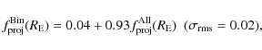
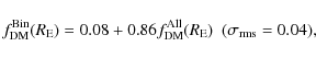
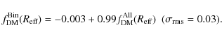
Considering that the typical uncertainties are much larger than the offsets and that the slopes of these relations are close to 1, we hereafter only considers the results from the fit to the full sample as our estimates of the DM mass fractions
We can further explore the viability of our results comparing our
estimated
![]() with previous estimates in literature.
Actually, a detailed comparison is not possible because our
systems are at an intermediate redshift (
with previous estimates in literature.
Actually, a detailed comparison is not possible because our
systems are at an intermediate redshift (
![]() ,
while dynamical and X-ray studies typically refer to nearby
galaxies. Moreover, such estimates are model dependent relying on
a given parametrization of the dark halo, while our constraints
come from a phenomenological and hence model independent analysis.
Since it is not possible to take quantitatively into account these
differences, we caution the reader to not overrate any agreement
or disagreement among our own and literature results.
,
while dynamical and X-ray studies typically refer to nearby
galaxies. Moreover, such estimates are model dependent relying on
a given parametrization of the dark halo, while our constraints
come from a phenomenological and hence model independent analysis.
Since it is not possible to take quantitatively into account these
differences, we caution the reader to not overrate any agreement
or disagreement among our own and literature results.
![\begin{figure}
\par\mbox{\subfigure{\includegraphics[width=8.08cm]{11090f3a.eps}...
...tomskip}
\subfigure{\includegraphics[width=8cm]{11090f3d.eps} }}
\end{figure}](/articles/aa/full_html/2009/36/aa11090-08/img511.png) |
Figure 3:
DM mass fractions and empirical M/L gradient vs total
luminosity |
| Open with DEXTER | |
As a first preliminary step, we briefly review some of the
previous determinations. An accurate quantitative estimate of
![]() has been obtained by Gerhard et al. (2001) from
a dynamical analysis of the line profiles of 21 mostly luminous,
slowly rotating and nearly round ETGs with well measured velocity
dispersion and circular velocity profiles. According to their
preferred minimum halo models, the DM mass fraction is
has been obtained by Gerhard et al. (2001) from
a dynamical analysis of the line profiles of 21 mostly luminous,
slowly rotating and nearly round ETGs with well measured velocity
dispersion and circular velocity profiles. According to their
preferred minimum halo models, the DM mass fraction is
![]() at the effective radius,
finding that their central dynamical M/L well agree with stellar
M/L estimated from synthetic models assuming a Salpeter IMF.
Using orbit superposition method, Thomas et al. (2005) managed to
reproduce in detail the observed kinematics of NGC 4807 finding
at the effective radius,
finding that their central dynamical M/L well agree with stellar
M/L estimated from synthetic models assuming a Salpeter IMF.
Using orbit superposition method, Thomas et al. (2005) managed to
reproduce in detail the observed kinematics of NGC 4807 finding
![]() taking for
taking for
![]() a guess from
populations synthesis models with a Kroupa IMF. A larger sample
of
24 ETGs with dynamics within
a guess from
populations synthesis models with a Kroupa IMF. A larger sample
of
24 ETGs with dynamics within
![]() reconstructed
from integral field spectroscopy was considered by Cappellari
et al. (2006).
Both two integrals analytic models and three integral
orbit superposition agree each other giving for
reconstructed
from integral field spectroscopy was considered by Cappellari
et al. (2006).
Both two integrals analytic models and three integral
orbit superposition agree each other giving for ![]() a median
value
a median
value
![]() using a Kroupa IMF as input to the estimate of
using a Kroupa IMF as input to the estimate of
![]() .
Analyzing a sample of local galaxies, Tortora et al.
(2009a) found that luminous galaxies have typical values of
.
Analyzing a sample of local galaxies, Tortora et al.
(2009a) found that luminous galaxies have typical values of
![]() ,
using a Salpeter IMF,
corresponding to
,
using a Salpeter IMF,
corresponding to
![]() for a Chabrier IMF. Finally,
stacking the same 22 lenses we are using, Gavazzi et al. (2007)
used a combined weak and strong lensing analysis leaving the
stellar M/L as a free parameter of the fit, finding out
for a Chabrier IMF. Finally,
stacking the same 22 lenses we are using, Gavazzi et al. (2007)
used a combined weak and strong lensing analysis leaving the
stellar M/L as a free parameter of the fit, finding out
![]() .
These authors estimate an
average value for stellar M/L of
.
These authors estimate an
average value for stellar M/L of
![]() (using h = 0.7),
which is 1.5 times the median value we obtain using a Chabrier
IMF. Renormalizing all the estimates to the Chabrier IMF, the
estimates for
(using h = 0.7),
which is 1.5 times the median value we obtain using a Chabrier
IMF. Renormalizing all the estimates to the Chabrier IMF, the
estimates for
![]() then span the range
then span the range
![]() .
Looking at Table 5, one can see that the values for
.
Looking at Table 5, one can see that the values for
![]() span a narrow range with
span a narrow range with
![]() averaging over the 21 lenses in the sample. Such a
value is in agreement with local estimates even if it is worth
noting that most of the lenses have values of
averaging over the 21 lenses in the sample. Such a
value is in agreement with local estimates even if it is worth
noting that most of the lenses have values of
![]() at
the upper end of the local range. Indeed, our estimates are on average
consistent with the local ones obtaibed in Tortora et al. (2009a)
when using the same Chabrier IMF adopted here. A more careful and
homogeneous (with respect to the local galaxies) sample is needed
to analyze the possible evolution of DM fraction
with redshift which is not the case here.
at
the upper end of the local range. Indeed, our estimates are on average
consistent with the local ones obtaibed in Tortora et al. (2009a)
when using the same Chabrier IMF adopted here. A more careful and
homogeneous (with respect to the local galaxies) sample is needed
to analyze the possible evolution of DM fraction
with redshift which is not the case here.
It has been recently reported in literature (Benson et al. 2000;
Marinoni & Hudson 2002; Graham & Guzman 2003; van den Bosch et al. 2003a,b; Napolitano et al. 2005; Tortora et al. 2009a,b) that
the DM content correlates with the total luminosity, with more
luminous (and massive galaxies) having higher values of
![]() .
This is what we indeed observe in
Fig. 3 where the projected and spherical DM mass
fractions (at both the Einstein and effective radii) are found to
correlate with
.
This is what we indeed observe in
Fig. 3 where the projected and spherical DM mass
fractions (at both the Einstein and effective radii) are found to
correlate with ![]() ,
with this latter quantity estimated at
the lens redshift. A direct fit, not taking into account
the errors, gives:
,
with this latter quantity estimated at
the lens redshift. A direct fit, not taking into account
the errors, gives:
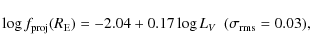
Note that the low scatter is actually far smaller than the typical uncertainty due to the errors on
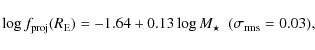
where
A different way of characterizing the galaxy DM content has been
proposed by Napolitano et al. (2005) introducing the empirical DM
gradient:
![\begin{displaymath}\nabla_l \Upsilon =
\frac{R_{\rm eff}}{r_{\rm out} - r_{\rm i...
... DM}(r)}{M_{\star}(r)} \right \vert _{r = r_{\rm in}} \right ]
\end{displaymath}](/articles/aa/full_html/2009/36/aa11090-08/img528.png)
which, for our model, reduces to:
 (1 + \eta_0)^{\beta}}.
\end{displaymath}](/articles/aa/full_html/2009/36/aa11090-08/img529.png)
We estimate this quantity for the lenses in our sample using the constraints from both the fit to the full lens sample and to the binned samples setting (
Figure 6 of Napolitano et al. (2005) plots the estimated
6.4 The impact of the IMF choice
All the results discussed insofar rely on the initial choice of
the stellar IMF. Adopting a different IMF, indeed, changes the
estimated stellar M/L ratios
![]() and hence the values of
and hence the values of
![]() and then of
and then of
![]() through Eq. (49). It is therefore worth wondering how the results
change with the IMF. To this aim, we rescale all the stellar M/L ratios by a factor 1.8, that is the same as assuming a Salpeter
rather than a Chabrier IMF. Then we repeat the fit to the full
sample with these rescaled
through Eq. (49). It is therefore worth wondering how the results
change with the IMF. To this aim, we rescale all the stellar M/L ratios by a factor 1.8, that is the same as assuming a Salpeter
rather than a Chabrier IMF. Then we repeat the fit to the full
sample with these rescaled
![]() and compare the best fit
parameters and the marginalized constraints with those in Table 2.
and compare the best fit
parameters and the marginalized constraints with those in Table 2.
Not surprisingly, we find a very good agreement for
![]() ,
while the only parameter changed is
,
while the only parameter changed is
![]() .
This can be easily understood considering that, for a
given lens, rescaling
.
This can be easily understood considering that, for a
given lens, rescaling
![]() is the same as rescaling
is the same as rescaling
![]() leaving unaltered the shape of the global M/L ratio
leaving unaltered the shape of the global M/L ratio
![]() .
In order to still fit the data, we have
therefore to retain the same functional expression and hence the
same values of the slope parameters
.
In order to still fit the data, we have
therefore to retain the same functional expression and hence the
same values of the slope parameters
![]() ,
but scale
,
but scale
![]() of the same amount as the
stellar M/L ratios. Since the luminosity is the same and the
virial mass has to remain unchanged in order to give the same
values of the projected mass and velocity dispersion, the virial
DM mass fraction has to be rescaled according to:
of the same amount as the
stellar M/L ratios. Since the luminosity is the same and the
virial mass has to remain unchanged in order to give the same
values of the projected mass and velocity dispersion, the virial
DM mass fraction has to be rescaled according to:
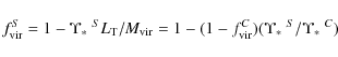
and for the mass scaling parameter we get:
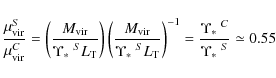
in agreement with what we find within the errors.
As a consequence, all the results obtained on the correlations
between the DM mass fractions and the stellar luminosity and mass
are still valid. Indeed, to take account of the change in the IMF,
we have simply to rescale the
![]() values using
values using
![]() ,
while
,
while
![]() has
to be increased by a constant factor
has
to be increased by a constant factor
![]() .
Both
these changes obviously rescales the corresponding zeropoints and
make the slope analyzed steeper than those obtained using a
Chabrier IMF strongly pointing to an increasing DM content as a
function of luminosity and stellar mass.
.
Both
these changes obviously rescales the corresponding zeropoints and
make the slope analyzed steeper than those obtained using a
Chabrier IMF strongly pointing to an increasing DM content as a
function of luminosity and stellar mass.
7 Conclusions
According to the estimated baryon and total matter density
parameter predicted by the cosmological concordance model, DM
should represent more than ![]() of the total matter budget. As
such, it is supposed to be ubiquitous representing therefore a
significant component of any galactic structure. Notwithstanding
this reasonable hypothesis, there is still a strong debate
regarding the DM content of ETGs with a variety of dynamical,
lensing and X-ray studies leading to contrasting results. The
lack of a reliable mass tracer in the ETGs outer regions and
modeling uncertainties make the problem of DM in ETGs a difficult
one to conclusively address. In order to reduce any possible
systematic bias due to the choice of the dark halo profile, a
phenomenological approach has been proposed in Tortora et al.
(2007) relying on the use of a versatile analytical expression for
the global M/L ratio
of the total matter budget. As
such, it is supposed to be ubiquitous representing therefore a
significant component of any galactic structure. Notwithstanding
this reasonable hypothesis, there is still a strong debate
regarding the DM content of ETGs with a variety of dynamical,
lensing and X-ray studies leading to contrasting results. The
lack of a reliable mass tracer in the ETGs outer regions and
modeling uncertainties make the problem of DM in ETGs a difficult
one to conclusively address. In order to reduce any possible
systematic bias due to the choice of the dark halo profile, a
phenomenological approach has been proposed in Tortora et al.
(2007) relying on the use of a versatile analytical expression for
the global M/L ratio
![]() .
Such a method allows to
smoothly interpolate between the two extreme cases of light
traces mass and dark halo dominance mimicking well the main
dynamical properties of a large class of intermediate models. As a
next mandatory step, we have here investigated the viability of
the model by contrasting it against the measured Einstein angles
and aperture velocity dispersions of a sample of 21 lenses
observed by the SLACS survey. A Bayesian statistical analysis
makes it possible to obtain the main results sketched below.
.
Such a method allows to
smoothly interpolate between the two extreme cases of light
traces mass and dark halo dominance mimicking well the main
dynamical properties of a large class of intermediate models. As a
next mandatory step, we have here investigated the viability of
the model by contrasting it against the measured Einstein angles
and aperture velocity dispersions of a sample of 21 lenses
observed by the SLACS survey. A Bayesian statistical analysis
makes it possible to obtain the main results sketched below.
- 1.
- The effective galaxy model obtained by combining our ansatz for
with the deprojection of the Sersic profile provided
by the Prugniel & Simien (1997) approximate expression is able to
reproduce the observations under the assumptions that the slope
parameters
 ,
the logarithmic slope of
the total density profile at the scaled Einstein radius,
,
the logarithmic slope of
the total density profile at the scaled Einstein radius,
 ,
and the virial mass ratio,
,
and the virial mass ratio,
 ,
are universal quantities, while the
model scalelelength
,
are universal quantities, while the
model scalelelength
 and global M/L ratio at
the effective radius
and global M/L ratio at
the effective radius
 may change on a case-by-case basis.
- 2.
- According to the marginalized constraints from the fit to the full
lens sample, the slope parameters
and
are in agreement
with what is expected in order the model mimics well cored halo profiles, while the
total density profile is locally approximated by an isothermal model as yet found
by previous studies in literature. We therefore argue that previous finding that an
isothermal model fits the lensing and dynamics data is likely a consequence of
having forced the total density profile to have a constant slope or of the data
covering a too limited radial range to detect the actual change in the logarithimic slope.
- 3.
- Binning the lenses according to their absolute V magnitude does not
improve the fit and, on the contrary, gives constraints on both
the model parameters and DM mass fractions that are in agreement
(within 68 or
 CL ranges) with those coming out from the
fit to the full lens sample. However, the small statistics and the
limited luminosity range probed does not allow us to draw any
definitive conclusion on the universality of the proposed
phenomenological
model.
CL ranges) with those coming out from the
fit to the full lens sample. However, the small statistics and the
limited luminosity range probed does not allow us to draw any
definitive conclusion on the universality of the proposed
phenomenological
model.
- 4.
- Using stellar population synthesis models and a Chabrier IMF
to estimate the stellar M/L ratios, we can constrain both the
projected and spherical DM mass fractions at the Einstein and
effective radii. Moreover, we have also estimated the empirical
M/L gradients proposed in Napolitano et al. (2005) as a
different way to quantify the DM content in ETGs.
- 5.
- There is a clear trend of
 with both
  and
and
 showing that the more luminous and/or massive a galaxy is, the
larger is its DM content within the effective radius. Unfortunately, the ranges in
and
probed are too small to make any quantitative
comparison with theoretical models.
showing that the more luminous and/or massive a galaxy is, the
larger is its DM content within the effective radius. Unfortunately, the ranges in
and
probed are too small to make any quantitative
comparison with theoretical models.
As a complementary approach, one can resort to a different class
of objects. Rather than concentrating on intermediate redshift
galaxies, nearby ETGs may be investigated relying on the velocity
dispersion profile to probe the model in the inner regions, while
planetary nebulae may extend deep in the outer regions thus
constraining the outer asymptotic slope. The analysis of the best
fit residuals here obtained has shown that no correlation with the
redshift is present thus suggesting that the model parameters
![]() do not evolve. Such a
conclusion must be, however, checked by both dividing lenses in
redshift bins and looking at a nearby sample. Should this result
be confirmed, one could then investigate what physical interplay
between stellar and dark components is able to give rise to a
global M/L ratio whose shape does not evolve with z. In
future analysis we will analyze this problem.
do not evolve. Such a
conclusion must be, however, checked by both dividing lenses in
redshift bins and looking at a nearby sample. Should this result
be confirmed, one could then investigate what physical interplay
between stellar and dark components is able to give rise to a
global M/L ratio whose shape does not evolve with z. In
future analysis we will analyze this problem.
As a final comment, we would like to stress the virtue of a phenomenological approach (not necessarily our own) to the problem of DM in ETGs. A comparison with the determination of the dark energy equation of state w(z) is worth doing here. Since a plethora of theoretically motivated models provide different expressions for w(z), it has soon become clear that fitting all of them to the different data available would be a prohibitive task. This lead to the emergence of phenomenological proposals for w(z) able to explore a wide range of models in a single step also providing model independent constraints to scrutinize different theories. Although the data on ETGs lensing and dynamics are still limited, it is nevertheless yet possible to rely on that positive experience to efficiently tackling the problem of DM in ETGs in a model independent way.
Acknowledgements
We warmly thank the referee for his/her constructive report which significantly helped us to improve the paper. V.F.C is supported by University of Torino and Regione Piemonte and partially from the INFN project PD51. C.T. is funded by a grant from the project Mecenas funded by the Compagnia di San Paolo.
References
- Benson, A. J., Cole, S., Frenk, C. S., Baugh, C. M., & Lacey, C. G. 2000, MNRAS, 311, 793 [NASA ADS] [CrossRef] (In the text)
- Binney, J. J., & Evans, N. W. 2001, MNRAS, 327, L27 [NASA ADS] [CrossRef]
- Bell, E. F., & de Jong, R. S. 2001, ApJ, 550, 212 [NASA ADS] [CrossRef]
- Bell, E. F., McIntosh, D. H., Katz, N., & Weinberg, M. D. 2003, ApJS, 149, 289 [NASA ADS] [CrossRef]
- Bolton, A. S., Burles, S., Koopmans, L. V. E., Treu, T., & Moustakas, L. A. 2006, ApJ, 638, 703 [NASA ADS] [CrossRef] (In the text)
- Bolton, A. S., Burles, S., Koopmans, L. V. E., et al. 2008, [arXiv:0805.1931] (In the text)
- Borriello, A., & Salucci, P. 2001, MNRAS, 323, 285 [NASA ADS] [CrossRef]
- Borriello, A., & Salucci, P., & Danese, L. 2003, MNRAS, 341, 1109 [NASA ADS] [CrossRef] (In the text)
- Bryan, G. L., & Norman, M. L. 1998, ApJ, 495, 80 [NASA ADS] [CrossRef]
- Bruzual, G., & Charlot, S. 2003, MNRAS, 344, 1000 [NASA ADS] [CrossRef] (In the text)
- Bullock, J. S., Kolatt, T. S., Sigad, Y., et al. 2001, MNRAS, 321, 559 [NASA ADS] [CrossRef] (In the text)
- Burkert, A. 1995, ApJ, 447, L25 [NASA ADS] [CrossRef] (In the text)
- Caon, N., Capaccioli, M., & D' Onofrio, M. 1993, MNRAS, 265, 1013 [NASA ADS] (In the text)
- Cappellari, M., Bacon, R., Bureau, M., et al. 2006, MNRAS, 366, 1126 [NASA ADS] (In the text)
- Cardone, V. F., Capozziello, S., Re, V., & Piedipalumbo, E. 2001 A&A, 379, 72
- Cardone, V. F., Capozziello, S., Re, V., & Piedipalumbo, E. 2002 A&A, 382, 792
- Cardone, V. F., Piedipalumbo, E., & v Tortora, C. 2005, MNRAS, 358, 1325 [NASA ADS] [CrossRef] (In the text)
- Chabrier, G. 2001, ApJ, 554, 1274 [NASA ADS] [CrossRef] (In the text)
- Ciotti, L., & Bertin, G. 1999, A&A, 352, 477 (In the text)
- Conroy, C., & Wechsler, R. H. 2008, [arXiv:0805.3346] (In the text)
- D' Agostini, G. 2004, [arXiv:physics/0403086]
- de Vaucouleurs, G. 1948, Ann. Astroph., 11, 247 [NASA ADS]
- Dunkley, J., Bucher, M., Ferreira, P. G., Moodley, K., & Skordis, C. 2005, MNRAS, 356, 925 [NASA ADS] [CrossRef] (In the text)
- Dunkley, J., Komatsu, E., Nolta, M. R., et al. 2009, ApJS, 180, 306 [NASA ADS] [CrossRef] (In the text)
- Einasto, J. 1965, Trudy Inst. Astrofiz. Alma - Ata, 5, 87 (In the text)
- Einasto, J., & Haud, U. 1989, A&A, 223, 89 [NASA ADS] (In the text)
- Fukushige, T., & Makino, J. 2001, ApJ, 557, 533 [NASA ADS] [CrossRef] (In the text)
- Gavazzi, R., Treu, T., Rhodes, J. D., et al. 2007, ApJ, 667, 176 [NASA ADS] [CrossRef] (In the text)
- Gerhard, O., Kronawitter, A., Saglia, R. P., & Bender, R. 2001, AJ, 121, 1936 [NASA ADS] [CrossRef] (In the text)
- Ghigna, S., Moore, B., Governato, F., et al. 2000, ApJ, 544, 616 [NASA ADS] [CrossRef] (In the text)
- Graham, A. W. 2002, MNRAS, 334, 859 [NASA ADS] [CrossRef]
- Graham, A. W., & Colless, M. 1997, MNRAS, 287, 221 [NASA ADS] (In the text)
- Graham, A. W., & Guzm
 n, R. 2003, AJ, 125, 2936 [NASA ADS] [CrossRef]
(In the text)
n, R. 2003, AJ, 125, 2936 [NASA ADS] [CrossRef]
(In the text) - Graham, A. W., & Driver, S. P. 2005, PASA, 22, 118 [NASA ADS] (In the text)
- Guzik, J., & Seljak, U. 2002, MNRAS, 335, 311 [NASA ADS] [CrossRef] (In the text)
- Jing, Y. P., & Suto, Y. 2000, ApJ, 529, L69 [NASA ADS] [CrossRef] (In the text)
- Kaviraj S., Kirkby, L. A., Silk, J., & Sarzi, M. 2007, MNRAS 382, 960 (In the text)
- Keeton, C. R., Kochanek, C. S., & Falco, E. E. 1998, ApJ, 509, 561 [NASA ADS] [CrossRef]
- Khalatyan A., Cattaneo A., Schramm M., et al. 2008, MNRAS, 387, 13 [NASA ADS] [CrossRef] (In the text)
- Kochanek, C. S. 1995, ApJ, 445, 559 [NASA ADS] [CrossRef]
- Koopmans, L. V. E., & Treu, T. 2003a, ApJ, 583, 606 [NASA ADS] [CrossRef] (In the text)
- Koopmans, L. V. E., & Treu, T. 2003b, ApJ, 599, 70 [NASA ADS] [CrossRef]
- Koopmans, L. V. E., Treu, T., Bolton, A. S., Burles, S., & Moustakas, L. A. 2006, ApJ, 649, 599 [NASA ADS] [CrossRef]
- Kroupa P. 2001, MNRAS, 322, 231 [NASA ADS] [CrossRef] (In the text)
- Loewenstein, M., & White, R. E. 1999 ApJ, 518, 50
- Márquez, I., Lima Neto, G. B., Capelato, H., et al. 2001, A&A, 379, 767 [NASA ADS] [CrossRef] [EDP Sciences] (In the text)
- Mamon, G. A., & Lokas, E. L. 2005a, MNRAS, 362, 95 [NASA ADS] [CrossRef] (In the text)
- Mamon, G. A., & Lokas, E. L. 2005b, MNRAS, 363, 705 [NASA ADS] [CrossRef]
- Mamon, G. A., Lokas, E. L., Dekel, A., Stoehr, F., & Cox, T. J. 2006, [astro-ph/0601345]
- Marinoni, C., & Hudson, M. J., 2002, ApJ, 569, 101 [NASA ADS] [CrossRef] (In the text)
- Mazure, A., & Capelato, H. V. 2002, A&A, 383, 384 [NASA ADS] [CrossRef] [EDP Sciences] (In the text)
- Merritt, D., Graham, A. W., Moore, B., Diemand, J., & Terzic, B. 2006, AJ, 132, 2685 [NASA ADS] [CrossRef] (In the text)
- Moore, B., Governato, F., Qinn, T., Stadel, J., & Lake, G. 1998, ApJ, 499, L5 [NASA ADS] [CrossRef] (In the text)
- Napolitano, N. R., Arnaboldi, M., Freeman, K. C., & Capaccioli, M. 2001, A&A, 377, 784 [NASA ADS] [CrossRef] [EDP Sciences] (In the text)
- Napolitano, N. R., Arnaboldi, M., & Capaccioli, M., 2002, A&A, 383, 791 [NASA ADS] [CrossRef] [EDP Sciences] (In the text)
- Napolitano, N. R., Capaccioli, M., Romanowsky, A. J., et al. 2005, MNRAS, 357, 691 [NASA ADS] [CrossRef] (In the text)
- Napolitano, N. R., et al. 2009, MNRAS, in preparation
- Navarro, J. F., Frenk, C. S., & White, S. D. M. 1996, ApJ, 462, 563 [NASA ADS] [CrossRef] (In the text)
- Navarro, J. F., Frenk, C. S., & White, S. D. M. 1997, ApJ, 490, 493 [NASA ADS] [CrossRef] (In the text)
- Navarro, J. F., Hayashi, E., Power, C., Jenkins, A. R., & Frenck, C. S. 2004, MNRAS, 349, 1039 [NASA ADS] [CrossRef] (In the text)
- Padmanabhan, N., Seljak, U., Strauss, M. A., et al. 2004, New Ast., 9, 329 [NASA ADS] [CrossRef] (In the text)
- Persic, M., Salucci, P., & Ashman, K. M. 1993, A&A, 279, 343 [NASA ADS] (In the text)
- Petters, A. O., Levine, H., & Wambsganss, J. 2001, Singularity theory and gravitational lensing, Birkhäuser, Boston (In the text)
- Power, C., Navarro, J. F., Jenkins, A., et al. 2003, MNRAS, 338, 14 [NASA ADS] [CrossRef] (In the text)
- Prugniel, Ph., & Simien, F. 1997, A&A, 321, 111 [NASA ADS] (In the text)
- Romanowsky, A. J., & Kochanek, C. S. 1997, MNRAS, 287, 95 [NASA ADS]
- Romanowsky, A. J., & Kochanek, C. S. 2001, ApJ, 553, 722 [NASA ADS] [CrossRef]
- Romanowsky, A. J., Douglas, N. G., & Arnaboldi, M. 2003, Science, 301, 1696 [NASA ADS] [CrossRef] (In the text)
- Ruszkowski M., & Springel V. 2009, [arXiv:0902.0373] (In the text)
- Salpeter, E. E. 1955, 121, 161 (In the text)
- Schawinski K., et al. 2008, [arXiv:0809.1096] (In the text)
- Schneider, P., Ehlers, J., & Falco, E. E. 1992, Gravitational lenses (Berlin: Springer-Verlag) (In the text)
- Sersic, J. L. 1968, Atlas de Galaxies Australes, Observatorio Astronomico de Cordoba (In the text)
- Shankar, F., & Bernardi, M. 2009, MNRAS, accepted, [arXiv:0903.3964] (In the text)
- Spergel, D. N., et al. ApJS, 2003, 148, 175 (In the text)
- Tortora, C., Cardone, V. F., & Piedipalumbo, E. 2007, A&A, 435, 107 (In the text)
- Tortora C., Antonuccio-Delogu V., Kaviraj S., et al. 2008a, MNRAS in press, [arXiv:0903.0397] (In the text)
- Tortora, C., Napolitano, N. R., Romanowsky, A. J., et al. 2009, [arXiv:0901.3781] (In the text)
- Tortora, C., et al. 2009b, in preparation
- Treu, T., & Koopmans, L. V. E. 2002a, MNRAS, 337, L6 [NASA ADS] [CrossRef] (In the text)
- Treu, T., & Koopmans, L. V. E. 2002b, ApJ, 575, 87 [NASA ADS] [CrossRef]
- Treu, T., & Koopmans, L. V. E. 2004, ApJ, 611, 739 [NASA ADS] [CrossRef] (In the text)
- van den Bosch, F. C., Yang, X., & Mo, H. J. 2003a, MNRAS, 340, 771 [NASA ADS] [CrossRef] (In the text)
- van den Bosch, F. C., Mo, H. J., & Yang, X. 2003b, MNRAS, 345, 923 [NASA ADS] [CrossRef]
- van den Bosch, F. C., Yang, X., Mo, H. J., et al. 2007, MNRAS, 376, 841 [NASA ADS] [CrossRef] (In the text)
- Winn, J. N., Rusin, D., & Kochanek, C. S. 2003, ApJ, 587, 80 [NASA ADS] [CrossRef]
- Winn, J. N., Rusin, D., & Kochanek, C. S. 2004, Nature, 427, 613 [NASA ADS] [CrossRef]
Footnotes
- ... radius
- Note that we have implicitly
assumed that the intensity I does not depend on the angular coordinates.
Actually, the isophotes are not concentric circles, but rather ellipses
with variable ellipticities and position angles so that
 .
However, in order to be consistent with our assumption of
spherical symmetry of the three dimensional mass profile, we will neglect
such an effect and, following a common practice, circularize the
intensity profile considering circular isophothes with radii equal to the
geometric mean of the major and minor axes.
.
However, in order to be consistent with our assumption of
spherical symmetry of the three dimensional mass profile, we will neglect
such an effect and, following a common practice, circularize the
intensity profile considering circular isophothes with radii equal to the
geometric mean of the major and minor axes.
- ... decay
- Actually, these are DM only simulations so that the addition of a baryonic component changes the global mass profile. Nevertheless, in the very outer regions, the stellar component may be neglected so that it is likely that the global mass profile behaves as the DM one thus recovering the exponential decay predicted by these simulations.
- ... defined
- A dimensional remark is in order
here. The deflection angle is expressed in arcsec so that,
although the effective radius
 is a length, in the right
hand side of Eq. (42), it must be expressed in
angular units.
is a length, in the right
hand side of Eq. (42), it must be expressed in
angular units.
- ...with
- Here, we recast the definition for deflection angle
and projected mass introducing the adimensional radius
 .
.
- ... preferred
- Note that the relation between the
concentration c and
is difficult to extract. Indeed, since we
set
as a result of fitting our phenomenological model to an input
stellar plus dark halo profile, its value also depends on the fitted
values of the other parameters,
 .
As a result,
we are therefore unable to say whether a larger
implies a higher
or smaller concentration.
.
As a result,
we are therefore unable to say whether a larger
implies a higher
or smaller concentration.
- ...
slopes
- Hereafter, we will consider
rather than
 as model parameter since it is this former
quantity that sets the asymptotic slope of the global M/L ratio.
Moreover, we have physically motivated constraints on
and
so that the ranges to be explored for these
parameters is immediately set. We also change from
as model parameter since it is this former
quantity that sets the asymptotic slope of the global M/L ratio.
Moreover, we have physically motivated constraints on
and
so that the ranges to be explored for these
parameters is immediately set. We also change from  to
as scalength parameter in order to explore a wider
range for this quantity.
to
as scalength parameter in order to explore a wider
range for this quantity.
- ...
choices
- While this is correct for a Salpeter IMF, since it differs from a Chabrier IMF only for the low mass slope and predict very similar colours, for a Kroupa IMF this is not strictly true, but we could assume the scale factor above as a good approximation.
- ... lens
- This is the lens identified as SDSS J234111.6+000019. In all the fits we will consider, this is, indeed, the lens showing the larger normalized residuals for both the projected mass and the velocity dispersion so that it is possible that some peculiar feature is at work. However, in order to not reduce the number of constraints without a definite motivation, we prefer to retain this object in the sample even if we caution the reader againt overrating its large residuals.
- ... values
- The high
 for B2 is due to
to the peculiar lens SDSS J234111.6+000019 so remember the caveat
yet quoted before.
for B2 is due to
to the peculiar lens SDSS J234111.6+000019 so remember the caveat
yet quoted before.
- ... fit
- Both in Fig. 2 and in the fits presented in this section, we first correct
for the small asymmetry in the errors following the prescriptions
given in D' Agostini (2004). Denoting with x the central value
and with
 the negative and positive error so that the
 CL reads
 ,
the corrected
value is
,
the corrected
value is
 with a symmetric
uncertainty
with a symmetric
uncertainty
 .
Note that,
since the
CL ranges in Table 5 are indeed quite symmetric, these
corrections are actually negligible for most of the lenses in our sample.
.
Note that,
since the
CL ranges in Table 5 are indeed quite symmetric, these
corrections are actually negligible for most of the lenses in our sample.
- ... fractions
- The complete set of constraints, including the ones from the fit to the binned samples, are available on request to the authors.
All Tables
Table 1: Photometric and lensing observables and estimated stellar M/L ratio for the 21 SLACS lenses.
Table 2: Results for the fit to the full lens sample.
Table 3: Results for the fit to the binned lenses.
Table 4: Marginalized constraints on the model parameters for different bins.
Table 5:
Median values and 68 and ![]() CL ranges for the DM mass fractions
using the chain for the fit to the full lens sample.
CL ranges for the DM mass fractions
using the chain for the fit to the full lens sample.
All Figures
| |
Figure 1:
Variation of the model parameters
with the median |
| Open with DEXTER | |
| In the text | |
| |
Figure 2:
Comparison between different DM content estimators as
constrained from the fit to the full or binned samples. Error bars
refer to the |
| Open with DEXTER | |
| In the text | |
| |
Figure 3:
DM mass fractions and empirical M/L gradient vs total
luminosity |
| Open with DEXTER | |
| In the text | |
Copyright ESO 2009
Current usage metrics show cumulative count of Article Views (full-text article views including HTML views, PDF and ePub downloads, according to the available data) and Abstracts Views on Vision4Press platform.
Data correspond to usage on the plateform after 2015. The current usage metrics is available 48-96 hours after online publication and is updated daily on week days.
Initial download of the metrics may take a while.