


| Issue |
A&A
Volume 711, July 2026
|
|
|---|---|---|
| Article Number | A234 | |
| Number of page(s) | 13 | |
| Section | Astrophysical processes | |
| DOI | https://doi.org/10.1051/0004-6361/202660232 | |
| Published online | 17 July 2026 | |
Time lags as a proxy of the spectral evolution in gamma-ray bursts
1
Dipartimento di Fisica e Chimica – Emilio Segrè, Università di Palermo, via Archirafi 36 - 90123 Palermo, Italy
2
INAF - Osservatorio Astronomica di Brera, Via E. Bianchi 46, I-23807 Merate (LC), Italy
3
Sorbonne Université, CNRS, UMR 7095, Institut d’Astrophysique de Paris, 98 Bis bd Arago, 75014 Paris, France
4
Institut Universitaire de France, Ministère de l’Enseignement Supérieur et de la Recherche, 1 rue Descartes, 75231 Paris Cedex F-05, France
5
INFN – Sezione di Milano–Bicocca, Piazza della Scienza 3, 20126 Milano (MI), Italy
6
INFN, Sezione di Trieste, I-34127 Trieste, Italy
★ Corresponding author: This email address is being protected from spambots. You need JavaScript enabled to view it.
Received:
3
April
2026
Accepted:
9
June
2026
Abstract
Context. Positive lags in gamma-ray bursts (GRBs) provide a unique window into the temporal evolution of their prompt emission, where hard photons precede softer ones. Negative lags, when hard photons are delayed, are instead harder to interpret. It is therefore critical to separate the different effects that produce the two types of lags for identifying the physical mechanisms at work in the prompt and early afterglow phases of GRBs.
Aims. We investigate the potential of time lags for distinguishing different emission components at different energy bands. Considering data from the Fermi Gamma-ray Burst Monitor (GBM) and the LAT Low Energy (LLE) technique, we establish a connection between lag behavior and high-energy spectral properties.
Methods. We performed a time-resolved joint spectral analysis in the range 10 keV–100 MeV for two exceptionally bright bursts, GRB 160625B and GRB 190114C. We computed the time lags between the lowest-energy band (10–100 keV) and progressively higher-energy bands up to 30–100 MeV for their distinct emission episodes by means of the cross-correlation function.
Results. For GRB 160625B, the spectra are described by a single component with clear hard-to-soft evolution, and the time lags are always positive. The analysis of the high-energy exponential cutoff, likely originating above the photosphere, yielded bulk Lorentz factor estimates of Γ ∼ 120 − 250. GRB 190114C exhibits negative lags in the 30–100 MeV band, coinciding with a delayed additional high-energy power-law component that begins to dominate the LLE range after ∼2.5 s. The comparison with multiwavelength observations showed some compatibility with the early afterglow, although its physical origin remains an open question that leaves room for interpretations such as external shocks or internal dissipation.
Conclusions. Time lags are effective diagnostic tools for investigating the spectral evolution of GRBs. Positive lags trace the softening of the prompt emission, whereas negative lags, although more difficult to interpret, indicate the appearance of a new, independent high-energy spectral component.
Key words: radiation mechanisms: non-thermal / gamma-ray burst: general / gamma-ray burst: individual: GRB 160625B / gamma-ray burst: individual: GRB 190114C
© The Authors 2026
 Open Access article, published by EDP Sciences, under the terms of the Creative Commons Attribution License (https://creativecommons.org/licenses/by/4.0), which permits unrestricted use, distribution, and reproduction in any medium, provided the original work is properly cited.
This article is published in open access under the Subscribe to Open model. This email address is being protected from spambots. You need JavaScript enabled to view it. to support open access publication.
1. Introduction
Gamma-ray bursts (GRBs) are short-lived flashes of γ-ray radiation originating at cosmological distances and releasing up to ∼1054 erg in isotropic equivalent energy. They are characterized by two distinct emission phases: an initial highly variable prompt emission of hard X-rays and γ-rays, followed by a multiwavelength afterglow that smoothly decays from very high energy (> 100 GeV) to radio frequencies (see Kumar & Zhang 2015; Nava 2021). GRBs are historically classified into long (> 2 s) and short (< 2 s) based on their prompt duration, which is linked to the collapse of massive stars and the merger of compact binaries, respectively1.
The physical mechanisms that cause the prompt emission remain highly uncertain. In the internal shock model, collisions between shells of different Lorentz factors within an ultra-relativistic outflow produce nonthermal radiation that accounts for the observed fast temporal variability (Rees & Mészáros 1994; Kobayashi et al. 1997; Daigne & Mochkovitch 1998). Alternatively, magnetic reconnection models invoke dissipation through reconnection events at large radii in highly magnetized outflows (Zhang & Yan 2011; McKinney & Uzdensky 2012; Beniamini & Granot 2016). Both models predict that the prompt emission originates above the photosphere, consistent with the observed nonthermal spectra. However, photospheric models have shown that dissipation near the photosphere can broaden a thermal spectrum into a nonthermal one, resembling the observed prompt spectra (Rees & Mészáros 2005; Pe’Er & Ryde 2017; Beloborodov & Mészáros 2017). Moreover, the possible presence of a component in addition to the usual prompt emission (Zhang et al. 2011) adds further complexity to this scenario and makes it crucial to identify and separate these contributions.
Time lags (or spectral lags), defined as the time delay between photons of different energies and measured via cross-correlation of GRB light curves (Band 1997; Peterson et al. 1998), are found to be a common feature of long GRBs, with magnitudes ranging from fractions of a second to tens of seconds (Norris et al. 2005; Chen et al. 2005; Ukwatta et al. 2010). Data from the Burst And Transient Source Experiment on board the Compton Gamma Ray Observatory showed that most long GRBs exhibit positive lags, with lower-energy photons arriving later, while only ∼10–20% show negative lags (Hakkila et al. 2007). Swift/BAT data confirmed positive or near-zero lags for long GRBs in the hard X-ray band (Ukwatta et al. 2010; Bernardini et al. 2015), whereas short GRBs exhibit negligible lags (Norris & Bonnell 2006; Zhang et al. 2006; Berger 2014; Bernardini et al. 2015). Above ∼100 MeV, observations with the Fermi Large Area Telescope (LAT) revealed a few negative lags between emission at MeV and GeV, either in individual bright bursts or in systematic studies of LAT-detected GRBs (Ackermann et al. 2013; Castignani et al. 2014; Ajello et al. 2019).
When a single emission component is present, positive lags are thought to arise from the hard-to-soft spectral evolution of the GRB spectrum (Kocevski & Liang 2003; Ryde 2005; Shao et al. 2017). The time lag behavior is indeed affected by the temporal evolution of the spectral and temporal parameters of the GRB during the propagation of the emitting region, such as its spectral indices, characteristic energies, shape, and spikiness of the light curves (Daigne & Mochkovitch 2003; Boçi et al. 2010; Mochkovitch et al. 2016). Positive time lags might also be affected by curvature effects associated with high-latitude emission from the relativistically expanding shell (Peng et al. 2011; Uhm & Zhang 2016). Negative lags are more complex to interpret: they have been proposed to signal the delayed emergence of an additional high-energy spectral component (Ackermann et al. 2013; Ajello et al. 2019), identified either as onset of the external afterglow (Gupta et al. 2021) or as inverse-Compton emission from internal shocks (Chakrabarti et al. 2018; Bošnjak et al. 2009; Bošnjak et al. 2009; Bošnjak & Daigne 2014). Time lags can therefore encode the spectral shape and its temporal evolution, making them a powerful diagnostic to probe GRB emission mechanisms, particularly when they are analyzed over a broad energy range.
Extracting meaningful information from time lags requires simultaneous observations over distinct non-overlapping energy bands, a capability enabled by the Fermi Gamma-ray Space Telescope. Through the synergy of the Gamma-ray Burst Monitor (GBM; Meegan et al. 2009) and the LAT (Atwood et al. 2009), continuous data coverage from 8 keV to over 100 GeV is provided. While the standard LAT data analysis considers photons with energies > 100 MeV, the LAT low-energy (LLE) technique is a more recent analysis that was developed to reconstruct photon energies from 30 to 100 MeV (Pelassa & Preece 2010). These data fill the gap between the GBM and the standard LAT energy ranges, thus allowing us to disentangle, if present, the prompt emission from the early afterglow component. The GeV emission detected by LAT has, in several cases, been interpreted as early afterglow radiation (Ghisellini et al. 2010; Ghirlanda et al. 2010; Abdo et al. 2009; Kumar & Duran 2010; Ajello et al. 2019).
In Maraventano et al. (2025), hereafter M25, the systematic analysis of 70 GRBs showed that time lags computed between the GBM-NaI (10–100 keV) and LLE (30–100 MeV) bands are positive in 40% of the bursts and negative in 37% of them, while the four short GRBs in the sample showed negligible lags. These results were interpreted within a simple phenomenological scenario, in which positive lags arise from the hard-to-soft spectral evolution of the prompt emission, while negative lags might be produced by the emergence of a distinct high-energy spectral component. However, this work only presented a time-integrated analysis of LLE spectra, so that it remains unclear whether positive lags reflect the hard-to-soft spectral evolution of the prompt emission and negative lags are truly associated with the delayed emergence of a high-energy component.
We investigate the potential of time lags as a complementary diagnostic tool for probing the emission mechanisms in GRBs, particularly in situations in which detailed spectral modeling is limited by poor photon statistics or data quality. Extending the analysis of M25, we perform a time-resolved joint GBM+LLE spectral study of two exceptionally bright Fermi bursts, GRBs 160625B and 190114C, selected for their high signal-to-noise ratio and broad energy coverage. These characteristics allowed us to track the spectral evolution and time-lag behavior across their distinct emission episodes with high sensitivity. We then examined the connection between spectral evolution and time lags and tested two physical scenarios: the hard-to-soft evolution of a single spectral component, and the delayed emergence of an independent high-energy component.
We describe the data selection and extraction in Section 2. The methods we adopted for computing time lags and performing time-resolved spectral analysis are presented in Section 3. We present the results in Section 4 and discuss them in Section 5. We give our conclusions in Section 6. Throughout the analysis process, we adopted the standard ΛCDM cosmology of Planck Collaboration VI (2020).
2. Data selection and extraction
In the following, we describe the criteria we used to select the two GRBs we analyzed, the extraction of their light curves and spectra from Fermi-GBM and LLE data, and the strategy for selecting time intervals for the time-resolved spectral analysis and time-lag computation.
2.1. Selected GRBs
We selected two bright Fermi GRBs: 160625B and 190114C. They both exhibit high LLE detection significance (49 and 53σ, respectively), as quantified by the Bayesian blocks algorithm (Ajello et al. 2019), and high photon statistics at lower energies, with fluences of 6.43 and 4.43 × 10⁻⁴ erg cm−2 in the 10–1000 keV band, corresponding approximately to the 85th and 76th percentiles of the GBM catalog fluence distribution (Von Kienlin et al. 2020). Both events also display light curves with several bright distinguishable pulses, enabling a detailed time-resolved joint GBM+LLE (10 keV–100 MeV) spectral analysis and time-lag computation between the lowest (10–100 keV) and highest (30–100 MeV) energy ranges allowed from the data.
2.2. Extracting light curves and spectra
For the two GRBs, we retrieved GBM time-tagged event (TTE) files from the Fermi online archive2 for the NaI and BGO detectors with the highest count rates. Photon events were binned at 0.1 s in three non-overlapping energy bands corresponding to the NaI (10–100 keV, Band 1), and BGO (150–500 keV, Band 2, and 500 keV–1 MeV, Band 3) detectors. For LAT/LLE data, TTE files were downloaded from the FERMILLE catalog3, pre-selected following Pelassa & Preece (2010), and filtered in the 30–100 MeV range (Band 4)4, also binned at 0.1 s. The background was estimated from off-source intervals before and after the GRB, fitted with polynomial functions up to the fourth order, with the best fit selected by the lowest χ2 and extrapolated over the burst interval. The light curves of GRBs 160625B and 190114C extracted in Bands 1, 2, 3, and 4 are shown in panels A–D of Fig. 1 and Fig. 2.
 |
Fig. 1. Time evolution of the spectral parameters and time lags obtained from the 2SBPLCUTOFF model (Table 1) for the time-resolved spectra of GRB 160625B. The vertical dashed gray lines indicate the time intervals adopted for the spectral analysis. Panels A–D display the count-rate light curves in Bands 1, 2, 3, and 4, binned at 0.1 s. Panel E shows the photon indices below the break, between the break and the peak energy, and above the peak energy (orange, yellow, and blue symbols, respectively). Panel F presents the temporal evolution of Epeak, Ebreak, and Ecutoff (red, blue, and green symbols, respectively). The light gray, blue, green, and orange shaded regions mark the energy ranges corresponding to Bands 1, 2, 3, and 4. Panel G shows the time lags between Band 1 and Bands 2, 3, and 4 (blue, green, and orange symbols, respectively; Table 3). Arrows indicate lower limits. |
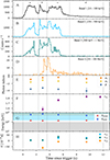 |
Fig. 2. Time evolution of the spectral parameters and time lags obtained from the 2SBPL+PL model (Table 2) for the time-resolved spectra of GRB 190114C. The vertical dashed gray lines indicate the time intervals adopted for the spectral analysis (in time bin a, only GBM data were considered). Panels A–D display the count-rate light curves in Bands 1, 2, 3, and 4, binned at 0.1 s. Panel E shows the photon indices below the break energy, between the break and the peak energies, and above the peak energy (orange, yellow, and blue symbols, respectively). Panel F shows the evolution of the photon index of the additional power-law component (purple symbols). Panel G presents the temporal evolution of Epeak and Ebreak (red and blue symbols, respectively). The light gray, blue, and green shaded regions mark the energy ranges corresponding to Bands 1, 2, and 3. Panel H shows the time lags between Band 1 and Bands 2, 3, and 4 (blue, green, and orange symbols, respectively; Table 3). |
The GBM and LLE spectral data products, including the response matrix files (rsp2), were retrieved from the online archive. Because the two GRBs are long-duration events, we used CSPEC data, with a temporal resolution of 1024 ms. The spectra were generated with the GTBURST5 software, covering 10–900 keV for NaI, 0.3–10 MeV for BGO, and 30–100 MeV for LLE. The channels between 30 and 40 keV were excluded to avoid systematic effects from the iodine K-edge at 33.17 keV6.
2.3. Time interval selection
Time intervals for the time-resolved spectral analysis were selected in a way to ensure a sufficient signal-to-noise ratio across all detectors. We first considered intervals that separated the distinct pulses in each GRB. Since the LLE data have the lowest photon statistics, we then ensured that each interval contained at least 50 LLE counts (in the 30–100 MeV band) after background subtraction. The same binning scheme was used for the time-lag computation. The selected intervals are listed in Table 1 for GRB 160625B and Table 2 for GRB 190114C. For GRB 160625B, the first pulse was split into its rise and decay sub-intervals, given its long duration and intensity (see Figure 1, panels A–D).
Best-fit parameters for the 2SBPLCUTOFF model for the time-integrated and time-resolved spectra of GRB 160625B.
3. Analysis
In this section, we describe the spectral models and the model-selection criterion adopted for the joint GBM+LLE spectral analysis of GRBs 160625B and 190114C, as well as the method used to compute the time lags between their distinct emission pulses. The time-integrated and time-resolved spectral analysis is presented in Section 3.1, while the time-lag computation method is described in Section 3.2.
3.1. GBM + LLE spectral analysis
The joint GBM+LLE time-integrated and time-resolved spectral analyses were performed with Xspec (version 12.14.1), adopting the Poissonian-Gaussian statistic (PG-STAT). We applied an intercalibration factor among all detectors, normalized to the NaI one, and allowed it to vary within 30%.
We modeled the spectra with a double smoothly broken power law (2SBPL; see Ravasio et al. 2018 for its functional form), consisting of three power laws with photon indices α1, α2, and β (from lowest to highest energies), connected at two break energies: Ebreak (separating the α1 and α2 power-law segments) and Epeak (separating the α2 and β segments). Since typically α2 > −2 and β < −2, Epeak represents the peak of the νFν spectrum.
For GRB 160625B, we investigated the presence of a high-energy spectral cutoff (as found in Ravasio et al. 2024 for the Fermi time-integrated spectrum from GBM to LAT energies) adopting the highecut multiplicative model from Xspec,
 (1)
(1)
where Ec is the cutoff onset energy, and Efold controls the sharpness of the transition. The model flux was reduced by a factor 1/e at Ecutoff = Ec + Efold, hereafter referred to as the cutoff energy. The resulting model (2SBPL × highecut) is denoted with 2SBPLCUTOFF.
For GRB 190114C, following Ajello et al. (2020), we tested the presence of an additional high-energy component by adding a power law (PL) to the 2SBPL,
 (2)
(2)
where NormPL is the normalization in units of photons keV−1cm−2s−1, and ΓPL is the photon index.
The best-fit model was chosen based on the Akaike information criterion (AIC; Akaike 1974): the more complex model (2SBPLCUTOFF or 2SBPL+PL) is preferred over the 2SBPL model when ΔAIC ≥ 6 (Burnham & Anderson 2004), where ΔAIC = AICi − AICmin is the difference between the AIC value of the ith model and the minimum AIC among the tested models7. All spectral parameter uncertainties are reported at 1σ confidence level.
3.2. Time-lag computation in different pulses
We estimated time lags between the lowest-energy GBM-NaI band (Band 1; 10–100 keV) and the three progressively higher-energy bands, GBM-BGO Band 2 (150–500 keV), Band 3 (500 keV–1 MeV), and LAT-LLE Band 4 (30–100 MeV). The corresponding time lags were denoted τ12, τ13, and τ14, and were computed over the full burst duration and over the same time intervals as were used for the time-resolved spectral analysis.
Following M25, time lags were computed via the discrete correlation function (DCF) method between pairs of background-subtracted light curves binned at 0.1 s. The lag τ is defined as the DCF maximum, determined by fitting the DCF with an asymmetric Gaussian, to account for the intrinsic asymmetry of GRB pulses, which allowed us to resolve lags smaller than the bin size. Uncertainties were estimated via a flux-randomization Monte Carlo technique (Peterson et al. 1998): for each energy band, N = 10 000 simulated light curves were generated by randomizing count rates according to their Poisson uncertainties, and the DCF was computed and fitted for each realization. The resulting τ distribution was fitted with a Gaussian, whose mean and standard deviation define the best-fit lag and its 1σ uncertainty. We note that this procedure only accounts for statistical uncertainties and does not capture systematic effects arising from overlapping pulses in multi-pulse light curves, which may bias the DCF toward incorrect lag values. This limitation is most relevant for time-integrated estimates and is mitigated by a time-resolved analysis, which isolates individual emission episodes. Furthermore, we caution that in the presence of overlapping emission components, the DCF lag can reflect a combination of contributions from different spectral components; its interpretation therefore strongly relies on spectral analysis results, as performed in this work.
4. Results
Tables 1 and 2 list the results of the joint GBM+LLE spectral analysis of GRBs 160625B and 190114C, respectively, including the time intervals, best-fit parameters, PG statistic over degrees of freedom, and ΔAIC = AICCOMPLEX − AIC2SBPL, where AICCOMPLEX refers to 2SBPLCUTOFF (GRB 160625B) or the 2SBPL+PL (GRB 190114C) related fit. Table 3 reports the time-lag results for the two GRBs, with the time bins and corresponding values of τ12, τ13, and τ14 with their uncertainties.
Best-fit parameters for the 2SBPL+PL model for the time-integrated and time-resolved spectra of GRB 190114C.
In the following, we discuss the spectral and time-lag evolution of each GRB, as well as the evidence of a high-energy cutoff in GRB 160625B and an additional power-law component in GRB 190114C. These results are then discussed in Section 5.
4.1. GRB 160625B
4.1.1. Time-integrated spectral analysis
We fitted the time-integrated spectrum of GRB 160625B over a 186–205 s interval from the trigger time8. The fit performed with the 2SBPLCUTOFF model yielded ΔAIC ∼ 96 with respect to the 2SBPL fit, confirming the presence of a high-energy spectral cutoff (Figure 3, top panel). In the following section, we expand this analysis by performing a time-resolved spectral analysis including Fermi-LLE data.
 |
Fig. 3. Time-integrated and time-resolved spectra of GRB 160625B in the 10 keV–100 MeV energy range fitted with the 2SBPLCUTOFF model (solid black line). The different colors correspond to the individual detectors, as indicated in the legend. In each panel, the lower strip displays the fit residuals. Arrows indicate lower limits. |
4.1.2. Time-resolved spectral analysis
Following Section 2, we divided the entire emission episode of GRB 160625B (186–205 s) into four time bins (a–d; dashed gray lines in Figure 1, panel A–D). The 2SBPL and 2SBPLCUTOFF models were fitted in each bin; the 2SBPLCUTOFF model was preferred in all bins (ΔAIC > 6), but only lower limits on Ecutoff were obtained in bins b and d. The best-fit model is shown in Figure 3 for each interval.
Figure 1 shows the light curves (panels A–D, binned at 0.1 s in Bands 1–4) and the temporal evolution of the 2SBPLCUTOFF parameters. The photon indices α1 and α2 are approximately constant over time, with mean values  and
and  , while β decreases over the first three bins, and
  . Although the compressed y-scale of panel F in Figure 1 makes it difficult to appreciate the spectral evolution visually, Epeak and Ebreak soften over time: Epeak decreases rapidly during the first ∼6 s and then decreases more slowly, while Ebreak drops sharply in the first ∼6 s before stabilizing around ∼145 keV. The evolution of Ecutoff is less straightforward; the lower limits in bins b and d suggest that the cutoff might lie above 100 MeV.
4.1.3. Time-lag analysis
Panel G of Figure 1 shows the evolution of τ12, τ13, and τ14 for GRB 160625B. All time lags are positive, indicating that high-energy photons systematically precede lower-energy photons across the full 10 keV–100 MeV range.
The values of τ12 and τ13 are mutually consistent and of order 10−2 s, as expected given the proximity in energy of Bands 2 and 3 and their common BGO detector, resulting in a closely related temporal structure of their light curves. In addition, the sensitivity of the DCF method might limit our ability to resolve small variations for time lags of this magnitude. In contrast, τ14 is systematically larger, up to an order of magnitude in the earliest bins, and it slowly decreases over time, suggesting an evolution of the dominant emission process or physical conditions of the emitting region at energies of hundreds of keV to MeV. This behavior is interpreted in Section 5 in the context of a single softening emission component, identified as the prompt. We also note that the burst-integrated lag values are higher than those measured in the individual time bins (Table 3), likely because the DCF applied to the full multi-peaked light curve correlates contributions from multiple overlapping pulses, inflating the resulting lag.
Time lags of GRB 160625B and 190114C, computed across their whole emission episode and in the same time bins as adopted for the spectral analysis, corresponding to separate pulses.
We also note that in intervals c and d, τ14 decreases to values comparable to or below τ12 and τ13. To further investigate this, we specifically computed the lags between Band 4 and Bands 2 and 3, τ24 and τ34, for these intervals. In bin c, we find τ24 = ( − 1 ± 3)×10−2 s and τ34 = ( − 2 ± 2)×10−2 s, while in bin d, τ24 = ( − 3 ± 3)×10−2 s and τ34 = ( − 3 ± 3)×10−2 s. While the central values of τ24 and τ34 are negative, they are all compatible with zero within 1σ, and no statistically significant lag inversion is therefore present within our energy range. In bin d, τ12, τ13, and τ14 are furthermore all mutually consistent within their uncertainties, indicating that the lag differences across all band pairs become negligible at late times.
4.2. GRB 190114C
4.2.1. Time-integrated spectral analysis
We fitted the time-integrated spectrum of GRB 190114C over the interval 0–12 s from the trigger time with a 2SBPL+PL model. The 2SBPL+PL is strongly preferred over the 2SBPL (ΔAIC ∼ 502; Table 2), with the power-law dominating in the LLE energy range at a photon index ΓPL ∼ 1.85, consistent with the LAT spectral slope above 100 MeV (Kocevski et al. 2019). The best-fit model is shown in Figure 4 (upper panel). We discuss the origin of this additional component in Section 5.
 |
Fig. 4. Time-integrated and time-resolved spectra of GRB 190114C in the 10 keV–100 MeV energy range fitted with the 2SBPL+PL model (solid black line). The dashed black line shows the 2SBPL model. The different colors correspond to the individual detectors, as indicated in the legend. In each panel, the lower strip displays the fit residuals. Arrows indicate upper limits. |
4.2.2. Time-resolved spectral analysis
We divided the 0–12 s interval into four bins (vertical dashed lines in Figure 2), separating the three distinct emission episodes visible in the light curve. In the first bin (0–2.3 s), LLE data were excluded because the signal was insufficient, and the spectrum is well described by a 2SBPL alone, with no evidence for an additional power-law component.
From ∼2.3 s onward, the 2SBPL+PL model is strongly preferred in all bins (ΔAIC > 100; see Table 2), with the power-law dominating at low energies from ∼10–30 keV, and then from a few tens of MeV across the entire LLE range (Figure 4). The value of ΓPL increases over time (Figure 2, panel F), with a mean value  over 2.3–12 s, consistent with the LAT measurement above 100 MeV and with the result of the time-integrated analysis. Of the 2SBPL parameters, Ebreak remains approximately constant around ∼141 keV, while Epeak decreases slowly (Figure 2, panel G); the photon indices α1, α2, and β show no clear temporal trend (Figure 2, panel E).
4.2.3. Time-lag analysis
The evolution of τ12, τ13, and τ14 for GRB 190114C is shown in panel H of Figure 2 and is listed in Table 3. No estimate of τ14 was possible in bin a because the LLE statistics are insufficient.
As for GRB 160625B, τ12 and τ13 are positive, of order 10−2 s, and mutually consistent; they increase with time, most notably in intervals b and c (∼3–7 s). In contrast, τ14 is negative in all bins and for the full emission episode, indicating that photons between 30–100 MeV systematically arrive after those at 10–100 keV. Its absolute value decreases sharply with time, from ∼ − 0.6 s in bin b to ∼ − 0.08 s in bin c, suggesting that the emission process and/or physical conditions evolve significantly between ∼3–7 s after the trigger. The burst-integrated value of τ14 is higher by an order of magnitude than the per-bin values, likely because the DCF incorrectly associates the bright early pulse visible only in the NaI and BGO light curves (∼2–5 s) with one of the later spiky pulses in the LLE light curve; when these episodes are separated into individual time bins, the inferred τ14 decreases dramatically.
5. Discussion
In this section, we interpret the time-lag and time-resolved spectral results of GRBs 160625B and 190114C (Sections 4.1 and 4.2), and we discuss the link between time lags and spectral evolution following the phenomenological scenario initially proposed in M25.
We considered two scenarios, depending on whether one or two spectral components dominated the emission in the considered energy bands.
(i) Single spectral component. Time lags arise naturally when a temporally evolving spectrum is observed through finite-width energy bands (Mochkovitch et al. 2016). For a single component undergoing hard-to-soft evolution, Epeak shifts progressively to lower energies, causing higher-energy light curves to peak earlier and producing positive lags, a well-established feature of long GRBs (Norris et al. 2000; Hakkila et al. 2007; Hafizi & Mochkovitch 2007; Mochkovitch et al. 2016). Crucially, Epeak does not need to cross the band boundaries to produce a measurable lag; continuous spectral softening within a band is sufficient, and this effect can become particularly pronounced when lags are computed between widely separated energy ranges (Castignani et al. 2014).
A high-energy exponential cutoff can modify this picture. If the cutoff remains well above the high-energy band, its effect on time lags is negligible; if it enters or crosses the band, it can suppress the high-energy light curve and produce negative lags. The temporal evolution of the cutoff depends on its physical origin: γγ pair-production opacity leads to a cutoff that rises with time as the outflow expands and becomes transparent (Ackermann et al. 2011; Granot et al. 2008; Yassine et al. 2017), initially suppressing high-energy photons and producing negative lags; conversely, in the fast-cooling regime and assuming that the acceleration timescale is proportional to the Larmor time, the observed cutoff energy associated with maximum electron Lorentz factor in the synchrotron component follows the evolution of the bulk Lorentz factor (see, e.g., Piran & Nakar 2010), leading to an expected decrease with time that can be reinforced if the IC cooling becomes important, determining the presence of a positive lag.
(ii) Two spectral components. When a second component contributes significantly at high energies, time lags no longer trace the evolution of a single component, but instead reflect the relative timing of distinct emission processes. The most common scenario is a delayed high-energy component, which may be of prompt origin or associated with the afterglow: if low-energy bands are dominated by the prompt emission alone while the high-energy band is dominated by a component that emerges later, the high-energy light curve peaks later, producing negative lags (Ackermann et al. 2013; Ajello et al. 2019; Bissaldi 2019). The opposite configuration of an early-peaking high-energy component is physically less natural as high-energy components from external shocks or opacity-regulated processes typically emerge progressively later than the main component.
In summary, positive lags most naturally indicate a single dominant component undergoing hard-to-soft spectral evolution, while negative lags are intrinsically more ambiguous: they may arise from an evolving γγ cutoff within a single component, or from the delayed onset of a second high-energy component. A joint spectral and temporal analysis is required to distinguish these scenarios.
5.1. GRB 160625B: Hard-to-soft evolution of a single component
The time-resolved spectral analysis of GRB 160625B shows that the emission is dominated throughout by a single 2SBPLCUTOFF component. Epeak and Ebreak both decrease with time, exhibiting a clear hard-to-soft evolution. The time lags are positive across the full 10 keV–100 MeV range: τ12 and τ13 are small and mutually consistent (∼10−2 s), while τ14 slowly decreases with time. This behavior is consistent with the hard-to-soft evolution of the prompt emission: the wider energy separation between the LLE and GBM bands amplifies the lag, and its gradual decrease reflects the slowing spectral evolution as Epeak shifts to lower energies at later times.
However, we note that in bins c and d, τ14 decreases to values lower than τ12 and τ13 (Table 3). To assess whether this implies a lag inversion between Band 4 and Bands 2–3, we specifically computed the lags τ24 and τ34 between Band 2/3 and Band 4 in these two intervals, respectively. While the values of τ24 and τ34 computed in intervals c and d are found to be negative, they are all compatible with zero within their uncertainties, so that no statistically significant lag inversion is detected between energy ranges involved in this work. We caution, however, that these results are affected by the limited photon statistics available at high energies in the LLE band, and higher-quality data are needed to draw more definitive conclusions on this point. We also note that a transition from positive to negative lags in GRB 160625B was previously reported by Wei et al. (2017), but they used energy bands extending up to LAT energies (> 100 MeV), that is, beyond the LLE range. The absence of a statistically significant inversion within our energy range is therefore consistent with the literature and with the single hard-to-soft component scenario we propose for GRB 160625B.
A natural explanation for this trend, within the single-component scenario, is suggested by the analytical model of Mochkovitch et al. (2016), who proposed that the sensitivity of a given lag to each spectral parameter depends on the position of the energy bands relative to Epeak: when both bands lie below Epeak, the lag is primarily controlled by the evolution of α1 and α2, whereas when one band lies above Epeak, the lag becomes sensitive to the evolution of β. In bins c and d, Band 4 (30–100 MeV) lies above Epeak (∼0.6–0.7 MeV), while Bands 1–3 remain below it, so that τ12 and τ13 are mainly governed by the evolution of α1 and α2, while τ14 is expected to be more sensitive to the evolution of β. According to this model, an increase in β might therefore reduce τ14 relative to τ12 and τ13. From interval c to d, β indeed slightly increases (Table 1).
The high-energy cutoff, detected at ∼100 MeV across all intervals, does not significantly affect the measured lags, since the LLE emission of GRB 160625B is concentrated between 30–60 MeV, well below the cutoff. Whether the cutoff arises due to γγ pair-production opacity or, in the case of the high-energy prompt emission, is due to IC scatterings from the intrinsic spectral shape of this additional component is investigated in Appendix A, where we estimate the bulk Lorentz factor Γ of the emitting region for these two assumptions. If the cutoff arises from photon–photon pair production, we find Γγγ ∼ 120 in the first interval, increasing to ∼230–260 in subsequent intervals, with a time-integrated value of Γγγ ≃ 230 (see Table A.1). The emission radius RMeV ∼ 1014 cm remains approximately constant in time and satisfies RMeV ≳ Rph ∼ 1013 cm in all intervals (Fig A.1, panel C), confirming that the prompt emission is produced in an optically thin region above the photosphere, as expected in internal shock or some magnetic reconnection scenarios. However, sub-photospheric models cannot be excluded on the basis of these constraints alone (Ryde et al. 2010; Ahlgren et al. 2019). If the cutoff reflects the intrinsic curvature of the IC spectrum, only lower limits on Γ can be derived; these closely track the Γγγ(Ecutoff) values while remaining systematically higher (Fig. A.1, panel B).
The case of GRB 160625B is consistent with a scenario in which the observed positive time lags are linked to the hard-to-soft spectral evolution of a single dominant emission component. The time-resolved spectral analysis identifies this component with the prompt emission, whose spectral properties and transparency condition suggest that the emission originates in an optically thin region above the photosphere.
5.2. GRB 190114C: Delayed emergence of a high-energy component
In GRB 190114C, an additional power-law spectral component emerges at ∼2.5 s after the trigger and dominates the LLE energy range and the soft X-ray energy range thereafter. Correspondingly, τ14 is negative in all time bins, indicating that 30–100 MeV photons arrive systematically later than those at 10–100 keV, while τ12 and τ13 remain positive and of order 10−2 s. The negative τ14 is thus a direct consequence of the delayed high-energy component and not the spectral evolution of the prompt.
A possible explanation for the additional component dominating at low and high energies is a contribution from an emerging afterglow emission. To test the consistency of this interpretation, we compared the flux of this spectral component with the flux of early-time afterglow emission. Observations from BAT and GBM showed a power-law decaying flux (starting from ∼25 s), interpreted as synchrotron afterglow radiation, whose smooth temporal decay forms an underlying continuum below the variability of the remaining prompt emission peaks (see the gray and gold crosses in Figure 5). The afterglow is also visible with XRT (although observations start at later times, ∼70 s) and LAT (0.1–1 GeV), although an indication of variability at early times questions a contribution from internal radiation up to ∼10 seconds, after which the GeV light curve is consistent with a smooth power-law temporal decay of external origin.
 |
Fig. 5. Light curves of GRB 190114C across different energy bands: Swift-XRT (light blue crosses), Swift-BAT (gray crosses), GBM (gold crosses), and Fermi-LAT data (filled red circles). The flux of the power-law component is shown with green (30–100 MeV) and yellow (10–30 keV) circles. The results obtained after dividing the first temporal bin into two sub-bins are shown with filled squares. The points represented by arrows indicate upper limits. |
To assess the consistency with afterglow emission of the additional power-law component present during the prompt emission, we estimated the flux of this additional component and compared it with early-time observations of afterglow radiation. We calculated the flux of the PL component in two specific energy ranges in which the power law dominates the 2SBPL component (see Figure 4): 10–30 keV and 30–100 MeV. Fluxes were calculated for all time intervals b–d defined in our time-resolved spectral analysis. Notably, we further divided bin b into two sub-intervals to better resolve the flux evolution within the first ∼3 s of the emission. In the first sub-bin, the additional PL component is not statistically required (i.e., the data are well described by a single 2SBPL model). In this case, we derived a 3σ upper limit to the power-law flux. This was computed by fixing the parameters obtained by the fit of the 2SBPL component and adding a power law with a fixed spectral index (see below) and increasing normalization until the fit worsened by a 3σ significance level compared to the pure 2SBPL model. The resulting normalization was used to calculate the flux upper limit in the two energy bands (10–30 keV and 30–100 MeV). For the spectral index of the power law, we considered the softest and hardest values obtained in the time-resolved analysis (ΓPL = 1.83 and 1.58) and selected the most conservative result on the flux upper limit derived. The resulting multi-wavelength light curves, including the flux of the power-law component in the 10–30 keV and 30–100 MeV bands, are shown in Figure 5.
Our multiwavelength comparison shows a good compatibility between the power-law flux and the afterglow emission observed by Swift, GBM, and Fermi-LAT. However, the rise of the power-law flux is very steep (steeper than t3), which differs from an interpretation as the onset of the afterglow. The physical nature of this component at early times remains uncertain and might require invoking a contribution from an internal high-energy component. Consequently, two physical interpretations remain viable. The additional component might be associated with the onset of the early afterglow from external shocks (Ravasio et al. 2019; Ronchi et al. 2020; Ajello et al. 2020), in which case the observed delay reflects the deceleration timescale of the outflow and the temporal evolution of τ14 might constrain the afterglow onset. Alternatively, the delayed component might arise from synchrotron self-Compton (SSC) emission within the same internal dissipation region as the prompt, with the delay driven by the evolving SSC efficiency (Daigne & Mochkovitch 2003; Bošnjak et al. 2009; Bošnjak & Daigne 2014) or the gradual reduction of early-time γγ opacity (Lithwick & Sari 2001; Hascoët et al. 2012; Yassine et al. 2017).
Regardless of the specific mechanism and the origin of the additional power-law component, the case of GRB 190114C illustrates the scenario in which negative time lags arise from different emission components dominating in different energy ranges. These results highlight the need for a joint spectral and temporal analyses to reliably interpret the origin of this component.
5.3. The case of a single spectral component with evolving HE absorption
A third scenario that is not applicable to any of the two GRBs we analyzed here ascribes negative lags to a single component whose high-energy cutoff evolves due to γγ opacity. In this scenario, no second spectral component is required. In this case, high-energy photons are initially suppressed by the high photon density of the compact emitting region, and they only escape as the outflow expands and becomes transparent, naturally producing negative lags.
No such case is found among the brightest GRBs in the sample of M25, that is, among those for which a spectral analysis can be performed, likely reflecting an observational bias. Measurable negative lags from a time-dependent γγ cutoff require high optical depths at early times, implying comparatively low bulk Lorentz factors (Lithwick & Sari 2001; Hascoët et al. 2012). Since Γ correlates with the isotropic-equivalent luminosity (Ghirlanda et al. 2010, 2018), low-Γ GRBs are intrinsically fainter and may not be feasible for a spectral analysis or even fall below the LLE detection threshold, introducing a natural bias against their inclusion in LLE-selected samples. A more quantitative assessment of the conditions under which evolving γγ opacity can generate observable negative lags and of the associated selection effects will be addressed in a dedicated theoretical study to be presented in a future work.
6. Conclusions
We have investigated the connection between time lags and spectral evolution in GRBs by combining joint GBM+LLE time-resolved spectral analyses with time-lag measurements for GRBs 160625B and 190114C, two bright Fermi events with high-quality broadband data from keV to tens of MeV and multiple distinct emission episodes. Building on the phenomenological framework of M25, we found that time lags measured between light curves in different energy bands provide a complementary, largely model-independent diagnostic of GRB spectral evolution. Unlike spectral fitting, which requires sufficient photon statistics and broad energy coverage, time lags can be robustly estimated even when detailed spectral modeling is not feasible, making them a valuable proxy for spectral evolution.
For GRB 160625B, the emission is dominated throughout by a single nonthermal component (2SBPLCUTOFF), with Ebreak and Epeak shifting to lower energies over time in a clear hard-to-soft evolution. All measured lags are positive across the full 10 keV–100 MeV range: τ12 and τ13 are small and comparable throughout all intervals, while τ14 is larger in the early intervals, but decreases to values comparable to or lower than τ12 and τ13 in bins c and d. According to the analytical model of lags from Mochkovitch et al. (2016), since Epeak always lies below the LLE band, τ14 is sensitive to the evolution of β throughout the burst, while τ12 and τ13 are primarily governed by the evolution of α1 and α2. The decrease of τ14 in bins c and d is therefore consistent with β increasing in these intervals, since this primarily affects τ14 without significantly changing τ12 and τ13. The lags τ24 and τ34 between Bands 2/3 and Band 4, computed in bins c and d, are all compatible with zero within 1σ, confirming that no statistically significant lag inversion is present at these energies. The high-energy cutoff near ∼100 MeV does not affect the lags, as the LLE emission is concentrated between 30–60 MeV and the transparency condition RMeV ≳ Rph is satisfied in all intervals (Table A.1). GRB 160625B therefore provides a case consistent with a scenario in which positive time lags are linked to the hard-to-soft spectral evolution of a single dominant prompt emission component.
For GRB 190114C, the low-energy emission is similarly described by a 2SBPL, but an additional power-law component emerges at ∼2.5 s and dominates the LLE range, so that time-integrated and time-resolved spectra require a 2SBPL+PL model. The lags τ12 and τ13 remain small and positive, suggesting that the keV–MeV emission is dominated by a single component, while τ14 is negative in all time bins, indicating that 30–100 MeV photons arrive systematically later. This behavior naturally arises when distinct spectral components dominate different energy bands. The delayed high-energy component might originate from external shocks (early afterglow) or from internal dissipation such as SSC emission, with early-time γγ opacity potentially contributing to the delay. Our multiwavelength comparison confirmed that the flux of this isolated power-law component is broadly consistent with the afterglow emission observed by Swift and Fermi-LAT, although early-time LAT variability suggests a more complex onset. Negative lags are therefore intrinsically more ambiguous than positive ones, and their interpretation requires a detailed spectral analysis combined with physical modeling. GRB 190114C nonetheless provides a clear example in which negative lags reflect the delayed emergence of a distinct high-energy spectral component.
We also found that none of the bright LLE-detected GRBs with negative τ14 in M25 can be modeled by a single spectral component alone. This is consistent with a natural observational bias: producing measurable negative lags in a single-component scenario requires a time-dependent γγ cutoff, implying low bulk Lorentz factors, and thus, intrinsically fainter bursts that are less likely to be detected or analyzed in the LLE range. A quantitative assessment of this scenario and its associated selection effects will be addressed in a future work.
Notably, 40% of the 70 GRBs in the M25 sample display a significantly positive τ14, suggesting that this lag behavior is common across the GRB population. Whether it universally reflects the same single-component hard-to-soft evolution as in GRB 160625B, however, cannot be established without a time-resolved spectral analysis of each individual burst, a task that is currently limited to the brightest LLE-detected events. Similarly, 37% of the M25 sample exhibit a significantly negative τ14, confirming that the delayed onset of a high-energy component is a recurring phenomenon. The physical origin of this behavior in each individual case, whether early afterglow emission, SSC radiation, or another process, remains to be determined through dedicated broadband spectral studies of the relevant subpopulation.
In conclusion, our results support a unified phenomenological picture in which positive time lags trace the hard-to-soft spectral evolution of a single dominant emission component, while negative lags most naturally signal the delayed emergence of an additional high-energy component. Time lags alone are insufficient to unambiguously identify the origin of the emission, but combined with a time-resolved spectral analysis, they constitute a powerful diagnostic of the physical processes at work. Future progress will benefit from larger GRB samples with high-quality broadband coverage, improved high-energy sensitivity, and joint temporal–spectral modeling with physically motivated emission models.
Acknowledgments
C.M. is grateful to the Institut d’astrophysique de Paris (IAP) for their warm hospitality during the course of this project. LN and GG acknowledge the European Union-Next Generation EU, PRIN 2022 RFF M4C21.1 (202298J7KT – PEACE). This work has been supported by the project GRB PrOmpt Emission Modular Simulator (POEMS) financed by INAF Grant 1.05.23.06.04.
References
- Abdo, A., Ackermann, M., Ajello, M., et al. 2009, ApJ, 706, L138 [NASA ADS] [CrossRef] [Google Scholar]
- Ackermann, M., Ajello, M., Asano, K., et al. 2011, ApJ, 729, 114 [CrossRef] [Google Scholar]
- Ackermann, M., Ajello, M., Asano, K., et al. 2013, ApJ, 763, 71 [CrossRef] [Google Scholar]
- Ahlgren, B., Larsson, J., Ahlberg, E., et al. 2019, MNRAS, 485, 474 [Google Scholar]
- Ajello, M., Arimoto, M., Axelsson, M., et al. 2019, ApJ, 878, 52 [NASA ADS] [CrossRef] [Google Scholar]
- Ajello, M., Arimoto, M., Axelsson, M., et al. 2020, ApJ, 890, 9 [Google Scholar]
- Akaike, H. 1974, IEEE Trans. Autom. Control, 19, 716 [Google Scholar]
- Atwood, W. B., Abdo, A. A., Ackermann, M., et al. 2009, ApJ, 697, 1071 [CrossRef] [Google Scholar]
- Band, D. L. 1997, ApJ, 486, 928 [Google Scholar]
- Beloborodov, A. M. 2013, ApJ, 764, 157 [NASA ADS] [CrossRef] [Google Scholar]
- Beloborodov, A., & Mészáros, P. 2017, Space Sci. Rev., 207, 87 [Google Scholar]
- Beniamini, P., & Granot, J. 2016, MNRAS, 459, 3635 [NASA ADS] [CrossRef] [Google Scholar]
- Berger, E. 2014, ARA&A, 52, 43 [CrossRef] [Google Scholar]
- Bernardini, M. G., Ghirlanda, G., Campana, S., et al. 2015, MNRAS, 446, 1129 [Google Scholar]
- Bissaldi, E. 2019, in ICRC 2019, ICRC, 36, 555 [Google Scholar]
- Boçi, S., Hafizi, M., & Mochkovitch, R. 2010, A&A, 519, A76 [NASA ADS] [CrossRef] [EDP Sciences] [Google Scholar]
- Bošnjak, Ž., & Daigne, F. 2014, ApJ, 568, A45 [Google Scholar]
- Bošnjak, Ž., Daigne, F., & Dubus, G. 2009, A&A, 498, 677 [NASA ADS] [CrossRef] [EDP Sciences] [Google Scholar]
- Bulla, M., Camisasca, A. E., Guidorzi, C., et al. 2023, GCN, 33578, 1 [Google Scholar]
- Burnham, K. P., & Anderson, D. R. 2004, Soc. Methods Res., 33, 261 [Google Scholar]
- Castignani, G., Guetta, D., Pian, E., et al. 2014, A&A, 565, A60 [NASA ADS] [CrossRef] [EDP Sciences] [Google Scholar]
- Chakrabarti, A., Chaudhury, K., Sarkar, S. K., & Bhadra, A. 2018, J. High Energy Astrophys., 18, 15 [Google Scholar]
- Chen, L., Lou, Y.-Q., Wu, M., et al. 2005, ApJ, 619, 983 [Google Scholar]
- Daigne, F., & Mochkovitch, R. 1998, MNRAS, 296, 275 [NASA ADS] [CrossRef] [Google Scholar]
- Daigne, F., & Mochkovitch, R. 2003, MNRAS, 342, 587 [NASA ADS] [CrossRef] [Google Scholar]
- Ghirlanda, G., Ghisellini, G., & Nava, L. 2010, A&A, 510, L7 [NASA ADS] [CrossRef] [EDP Sciences] [Google Scholar]
- Ghirlanda, G., Nappo, F., Ghisellini, G., et al. 2018, A&A, 609, A112 [NASA ADS] [CrossRef] [EDP Sciences] [Google Scholar]
- Ghisellini, G., Ghirlanda, G., Nava, L., & Celotti, A. 2010, MNRAS, 403, 926 [NASA ADS] [CrossRef] [Google Scholar]
- Golkhou, V. Z., Butler, N. R., & Littlejohns, O. M. 2015, ApJ, 811, 93 [NASA ADS] [CrossRef] [Google Scholar]
- Granot, J., Cohen-Tanugi, J., & do Couto e Silva, E. 2008, ApJ, 677, 92 [NASA ADS] [CrossRef] [Google Scholar]
- Gupta, R., Oates, S., Pandey, S., et al. 2021, MNRAS, 505, 4086 [NASA ADS] [Google Scholar]
- Hafizi, M., & Mochkovitch, R. 2007, A&A, 465, 67 [NASA ADS] [CrossRef] [EDP Sciences] [Google Scholar]
- Hakkila, J., Giblin, T. W., Young, K. C., et al. 2007, ApJS, 169, 62 [NASA ADS] [CrossRef] [Google Scholar]
- Hascoët, R., Daigne, F., Mochkovitch, R., & Vennin, V. 2012, MNRAS, 421, 525 [NASA ADS] [Google Scholar]
- Kobayashi, S., Piran, T., & Sari, R. 1997, ApJ, 490, 92 [Google Scholar]
- Kocevski, D., & Liang, E. 2003, ApJ, 594, 385 [Google Scholar]
- Kocevski, D., Omodei, N., Axelsson, M., et al. 2019, GCN, 23709, 1 [Google Scholar]
- Kumar, P., & Duran, R. B. 2010, MNRAS, 409, 226 [NASA ADS] [CrossRef] [Google Scholar]
- Kumar, P., & Zhang, B. 2015, Phys. Rep., 561, 1 [Google Scholar]
- Lithwick, Y., & Sari, R. 2001, ApJ, 555, 540 [NASA ADS] [CrossRef] [Google Scholar]
- Maraventano, C., Ghirlanda, G., Nava, L., et al. 2025, A&A, 697, A161 [NASA ADS] [CrossRef] [EDP Sciences] [Google Scholar]
- McKinney, J. C., & Uzdensky, D. A. 2012, MNRAS, 419, 573 [Google Scholar]
- Meegan, C., Lichti, G., Bhat, P., et al. 2009, ApJ, 702, 791 [NASA ADS] [CrossRef] [Google Scholar]
- Mochkovitch, R., Heussaff, V., Atteia, J., Boçi, S., & Hafizi, M. 2016, A&A, 592 [Google Scholar]
- Nava, L. 2021, Universe, 7, 503 [NASA ADS] [CrossRef] [Google Scholar]
- Norris, J. P., & Bonnell, J. T. 2006, ApJ, 643, 266 [NASA ADS] [CrossRef] [Google Scholar]
- Norris, J., Marani, G., & Bonnell, J. 2000, ApJ, 534, 248 [NASA ADS] [CrossRef] [Google Scholar]
- Norris, J. P., Bonnell, J. T., Kazanas, D., et al. 2005, ApJ, 627, 324 [NASA ADS] [CrossRef] [Google Scholar]
- Pe’Er, A., & Ryde, F. 2017, Int. J. Mod. Phys. D, 26, 1730018 [Google Scholar]
- Pe’er, A., Ryde, F., Wijers, R. A., Mészáros, P., & Rees, M. J. 2007, ApJ, 664 [Google Scholar]
- Pelassa, V., & Preece, R. 2010, arXiv e-prints [arXiv:1002.2617] [Google Scholar]
- Peng, Z., Yin, Y., Bi, X., Bao, Y., & Ma, L. 2011, AN, 332, 92 [Google Scholar]
- Peterson, B. M., Wanders, I., Horne, K., et al. 1998, PASP, 110, 660 [Google Scholar]
- Piran, T., & Nakar, E. 2010, ApJ, 718, L63 [NASA ADS] [CrossRef] [Google Scholar]
- Planck Collaboration VI. 2020, A&A, 641, A6 [NASA ADS] [CrossRef] [EDP Sciences] [Google Scholar]
- Ravasio, M., Oganesyan, G., Ghirlanda, G., et al. 2018, A&A, 613, A16 [NASA ADS] [CrossRef] [EDP Sciences] [Google Scholar]
- Ravasio, M., Oganesyan, G., Salafia, O., et al. 2019, A&A, 626, A12 [NASA ADS] [CrossRef] [EDP Sciences] [Google Scholar]
- Ravasio, M., Ghirlanda, G., & Ghisellini, G. 2024, A&A, 685, A166 [NASA ADS] [CrossRef] [EDP Sciences] [Google Scholar]
- Rees, M. J., & Mészáros, P. 1994, ApJ, 430, L93 [Google Scholar]
- Rees, M. J., & Mészáros, P. 2005, ApJ, 628, 847 [NASA ADS] [CrossRef] [Google Scholar]
- Ronchi, M., Fumagalli, F., Ravasio, M., et al. 2020, A&A, 636, A55 [NASA ADS] [CrossRef] [EDP Sciences] [Google Scholar]
- Rossi, A., Rothberg, B., Palazzi, E., et al. 2022, ApJ, 932, 1 [NASA ADS] [CrossRef] [Google Scholar]
- Ryde, F. 2005, A&A, 429, 869 [NASA ADS] [CrossRef] [EDP Sciences] [Google Scholar]
- Ryde, F., Axelsson, M., Zhang, B., et al. 2010, ApJ, 709, L172 [Google Scholar]
- Shao, L., Zhang, B.-B., Wang, F.-R., et al. 2017, ApJ, 844, 126 [Google Scholar]
- Uhm, Z. L., & Zhang, B. 2016, ApJ, 824, L16 [CrossRef] [Google Scholar]
- Ukwatta, T., Stamatikos, M., Dhuga, K., et al. 2010, ApJ, 711, 1073 [NASA ADS] [CrossRef] [Google Scholar]
- Von Kienlin, A., Meegan, C. A., Paciesas, W. S., et al. 2020, ApJ, 893, 46 [NASA ADS] [CrossRef] [Google Scholar]
- Wei, J. J., Zhang, B. B., Shao, L., Wu, X. F., & Mészáros, P. 2017, ApJ, 834 [Google Scholar]
- Xu, D., Malesani, D., Fynbo, J. P. U., et al. 2016, GCN, 19600, 1 [Google Scholar]
- Yassine, M., Piron, F., Mochkovitch, R., & Daigne, F. 2017, A&A, 606, A93 [NASA ADS] [CrossRef] [EDP Sciences] [Google Scholar]
- Zhang, B., & Yan, H. 2010, ApJ, 726, 90 [Google Scholar]
- Zhang, B., & Yan, H. 2011, ApJ, 726, 90 [Google Scholar]
- Zhang, Z., Xie, G., Deng, J., & Jin, W. 2006, MNRAS, 373, 729 [NASA ADS] [CrossRef] [Google Scholar]
- Zhang, B.-B., Zhang, B., Liang, E.-W., et al. 2011, ApJ, 730, 141 [NASA ADS] [CrossRef] [Google Scholar]
- Zhong, S.-Q., Li, L., & Dai, Z.-G. 2023, ApJ, 947, L21 [NASA ADS] [CrossRef] [Google Scholar]
The recent discovery of long GRBs with a compact binary progenitor (Zhong et al. 2023; Bulla et al. 2023) and vice versa (Rossi et al. 2022) increasingly challenges this traditional classification.
These four non-overlapping bands follow the same scheme as M25, ensuring adequate photon statistics while tracking time lag evolution with energy.
The relative likelihood of the ith model is e−ΔAIC/2; for ΔAIC = 6, this corresponds to ∼0.05, meaning that the ith model is about 20 times less probable than the best-fit model.
The precursor was excluded from this fit.
Appendix A: Estimation of the Lorentz factor for GRB 160625B
The high-energy exponential cutoff observed in the time-integrated and time-resolved spectra of GRB 160625B (see Table 1 and Figure 3) can be interpreted in two ways: if the cutoff arises from photon–photon pair production (γγ → e+e−), the bulk Lorentz factor Γ of the emitting region can be directly estimated (Lithwick & Sari 2001; Pe’er et al. 2007; Hascoët et al. 2012; Yassine et al. 2017; Ravasio et al. 2024). In the hypothesis that the high-energy prompt-emission spectrum is associated with an IC origin, the spectral break can reflect an intrinsic spectral curvature from IC scattering in the Klein–Nishina regime (hereafter natural break); in this case, only a lower limit on Γ can be derived In this section, we estimate Γ for both scenarios following the methodology presented in Yassine et al. (2017), assuming throughout that the prompt emission originates above the photosphere in an optically thin regime, and verifying this assumption a posteriori.
Case (i): Cutoff due to γ-ray opacity to pair creation
In the optically thin regime, the radius at which MeV photons are produced is given by
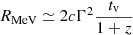 (A.1)
(A.1)
valid for internal shocks (Daigne & Mochkovitch 1998; Rees & Mészáros 2005) and some magnetic reconnection models (e.g., ICMART, Zhang & Yan 2010). If the high-energy cutoff is due to photon opacity to pair creation, the bulk Lorentz factor Γγγ is then estimated from Hascoët et al. (2012):
![Mathematical equation: $$ \begin{aligned} \begin{split} \Gamma _{\gamma \gamma } = \frac{K \Phi (s)}{\left[\frac{1}{2}\left(1 + \frac{R_{\mathrm{GeV} }}{R_\mathrm{MeV} }\right) \left(\frac{R_{\mathrm{GeV} }}{R_\mathrm{MeV} }\right)\right]^{1/2}}\,\,\left(1 + z\right)^{-(1+s)/(1-s)} \times \\ \times \,\left\{ \sigma _\mathrm{T} \left[\frac{D_\mathrm{L} (z)}{c\,t_{\mathrm{v} }}\right]^2 E_* F(E_*)\right\} ^{1/2(1-s)}\left[\frac{E_*E_\mathrm{cut} }{(m_ec^2)^2}\right]^{(s+1)/2(s-1)}, \end{split} \end{aligned} $$](/articles/aa/full_html/2026/07/aa60232-26/aa60232-26-eq79.gif) (A.2)
(A.2)
where σT is the Thomson cross section, DL = 3.17 × 1028 cm is the luminosity distance at z = 1.406 (Xu et al. 2016). The constant K ≃ 0.4–0.5 is calibrated via numerical calculations of the γγ opacity process (Hascoët et al. 2012); we let K vary across this range and adopt the corresponding average Γγγ as our result. For simplicity, we allow the variability timescale tv to vary within the range 0.1–1 s, which is consistent with what is obtained for long Fermi GRBs (Golkhou et al. 2015). We also assume that MeV and GeV photons are produced in the same region (RMeV ≃ RGeV).
The quantities needed to compute Γγγ are listed in Table A.1: Ecutoff is the cutoff obtained from the 2SBPLCUTOFF fit; E*, the characteristic seed photon energy interacting with cutoff-energy photons (Eq. 8 in Yassine et al. 2017); F(E*), the photon fluence at E* over tv; s, the local photon index around E*; and Φ(s), a function of s alone (Eqs. 9–10 in Yassine et al. 2017). Since the seed spectrum is locally a power law, Γγγ is insensitive to the specific choice of E*. The index s was estimated via Monte Carlo sampling of the covariance matrix from the 2SBPLCUTOFF fits. Similarly, the corresponding values of F(E*) were obtained directly from the spectral fits.
Spectral parameters and results of the Lorentz factor computation, for all the time-intervals of GRB 160625B analyzed.
The resulting Γγγ(Ecutoff) and RMeV values are shown in Figure A.1 (green and yellow symbols, respectively) and listed in Table A.1. The bulk Lorentz factor increases from ∼120 in interval a to ∼230–260 in subsequent intervals; lower limits apply in intervals b and d where Ecutoff is unconstrained. The time-integrated value Γγγ ≃ 230 is consistent with the time-resolved average. The emission radius RMeV ∼ 1014 cm is approximately constant across intervals, with lower limits in intervals b and d.
 |
Fig. A.1. Time evolution of the Lorentz factor and characteristic radii, for the time-resolved spectra of GRB 160625B. Vertical gray dashed lines indicate the time intervals adopted for the spectral analysis. Panel A displays the count-rate light curve in the full NaI energy range, binned at 0.1 s. Panel B shows the Lorentz factors measured assuming that the high-energy cutoff at Ecutoff is either due to gamma-gamma opacity to pair production, or a natural break of the emission mechanisms (green and red symbols, respectively). Panel C presents the evolution of the radius at which the MeV photons are produced, and the photospheric radius (yellow and orange symbols, respectively). Arrows indicate upper or lower limits. |
To verify the self-consistency of the optically thin assumption, we compare Γγγ with the minimum Lorentz factor required for transparency to Thomson scattering, using the photospheric radius (Beloborodov 2013):
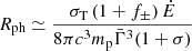 (A.3)
(A.3)
where 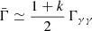 is the mean outflow Lorentz factor (with k ∼ 2–5 being the contrast factor; Hascoët et al. 2012); f± is the pair-to-electron ratio, which vanishes when the pair-creation optical depth is below unity at RMeV (which is verified for all intervals); Ė = L/ϵrad is the total injected power, with the observed γ-ray luminosity L given in Table A.1, radiative efficiency of the prompt ϵrad = 0.1; and magnetization parameter σ ≪ 1 in the internal-shock scenario.
The transparency condition RMeV ≥ Rph is satisfied in all intervals (Figure A.1, panel C; Table A.1), with RMeV ∼ 1014 cm and Rph ∼ 1013 cm, confirming that the prompt emission is consistent with dissipation well above the photosphere, as expected in internal shock or some magnetic reconnection scenarios. We note, however, that satisfying the transparency condition does not exclude photospheric models, since sub-photospheric dissipation followed by radiative transfer could produce emission at comparable radii. However, an in-depth assessment of this alternative relies on detailed modeling of radiative transfer across the photosphere, which is beyond the scope of this work.
Case (ii): Cutoff due to a natural break in the spectrum
We now briefly consider an alternative interpretation, in which the observed high-energy cutoff reflects the intrinsic curvature of the inverse Compton spectrum rather than being caused by γγ pair production opacity. In this scenario, the cutoff arises naturally from the radiative process, and only a lower limit on the Lorentz factor can be derived. In each time interval, we have
![Mathematical equation: $$ \begin{aligned} \Gamma _\mathrm{LL} = \max [\Gamma _{\gamma \gamma }(E_\mathrm{max} )\,,\, \Gamma _\mathrm{tr} ] \end{aligned} $$](/articles/aa/full_html/2026/07/aa60232-26/aa60232-26-eq85.gif) (A.4)
(A.4)
where Emax is the maximum photon energy detected in each time interval (see Table A.1), and Γtr is the lower limit of the Lorentz factor for transparency. Since RMeV ≥ Rph for all intervals, then Γγγ(Emax) ≥ Γtr. The resulting lower limits are shown in Figure A.1 (red symbols) and listed in Table A.1. We find that these limits closely track the values of Γγγ(Ecutoff), while being always larger.
The results presented in this section allow us to test the proposed phenomenological scenario discussed in Section 5, in which the relation of time lags and spectral evolution for GRB 160625B is investigated in terms of the prompt emission of internal origin, which evolves hard to soft over time, and on the presence of the high-energy cutoff.
All Tables
Best-fit parameters for the 2SBPLCUTOFF model for the time-integrated and time-resolved spectra of GRB 160625B.
Best-fit parameters for the 2SBPL+PL model for the time-integrated and time-resolved spectra of GRB 190114C.
Time lags of GRB 160625B and 190114C, computed across their whole emission episode and in the same time bins as adopted for the spectral analysis, corresponding to separate pulses.
Spectral parameters and results of the Lorentz factor computation, for all the time-intervals of GRB 160625B analyzed.
All Figures
|
Fig. 1. Time evolution of the spectral parameters and time lags obtained from the 2SBPLCUTOFF model (Table 1) for the time-resolved spectra of GRB 160625B. The vertical dashed gray lines indicate the time intervals adopted for the spectral analysis. Panels A–D display the count-rate light curves in Bands 1, 2, 3, and 4, binned at 0.1 s. Panel E shows the photon indices below the break, between the break and the peak energy, and above the peak energy (orange, yellow, and blue symbols, respectively). Panel F presents the temporal evolution of Epeak, Ebreak, and Ecutoff (red, blue, and green symbols, respectively). The light gray, blue, green, and orange shaded regions mark the energy ranges corresponding to Bands 1, 2, 3, and 4. Panel G shows the time lags between Band 1 and Bands 2, 3, and 4 (blue, green, and orange symbols, respectively; Table 3). Arrows indicate lower limits. |
| In the text | |
|
Fig. 2. Time evolution of the spectral parameters and time lags obtained from the 2SBPL+PL model (Table 2) for the time-resolved spectra of GRB 190114C. The vertical dashed gray lines indicate the time intervals adopted for the spectral analysis (in time bin a, only GBM data were considered). Panels A–D display the count-rate light curves in Bands 1, 2, 3, and 4, binned at 0.1 s. Panel E shows the photon indices below the break energy, between the break and the peak energies, and above the peak energy (orange, yellow, and blue symbols, respectively). Panel F shows the evolution of the photon index of the additional power-law component (purple symbols). Panel G presents the temporal evolution of Epeak and Ebreak (red and blue symbols, respectively). The light gray, blue, and green shaded regions mark the energy ranges corresponding to Bands 1, 2, and 3. Panel H shows the time lags between Band 1 and Bands 2, 3, and 4 (blue, green, and orange symbols, respectively; Table 3). |
| In the text | |
|
Fig. 3. Time-integrated and time-resolved spectra of GRB 160625B in the 10 keV–100 MeV energy range fitted with the 2SBPLCUTOFF model (solid black line). The different colors correspond to the individual detectors, as indicated in the legend. In each panel, the lower strip displays the fit residuals. Arrows indicate lower limits. |
| In the text | |
|
Fig. 4. Time-integrated and time-resolved spectra of GRB 190114C in the 10 keV–100 MeV energy range fitted with the 2SBPL+PL model (solid black line). The dashed black line shows the 2SBPL model. The different colors correspond to the individual detectors, as indicated in the legend. In each panel, the lower strip displays the fit residuals. Arrows indicate upper limits. |
| In the text | |
|
Fig. 5. Light curves of GRB 190114C across different energy bands: Swift-XRT (light blue crosses), Swift-BAT (gray crosses), GBM (gold crosses), and Fermi-LAT data (filled red circles). The flux of the power-law component is shown with green (30–100 MeV) and yellow (10–30 keV) circles. The results obtained after dividing the first temporal bin into two sub-bins are shown with filled squares. The points represented by arrows indicate upper limits. |
| In the text | |
|
Fig. A.1. Time evolution of the Lorentz factor and characteristic radii, for the time-resolved spectra of GRB 160625B. Vertical gray dashed lines indicate the time intervals adopted for the spectral analysis. Panel A displays the count-rate light curve in the full NaI energy range, binned at 0.1 s. Panel B shows the Lorentz factors measured assuming that the high-energy cutoff at Ecutoff is either due to gamma-gamma opacity to pair production, or a natural break of the emission mechanisms (green and red symbols, respectively). Panel C presents the evolution of the radius at which the MeV photons are produced, and the photospheric radius (yellow and orange symbols, respectively). Arrows indicate upper or lower limits. |
| In the text | |
Current usage metrics show cumulative count of Article Views (full-text article views including HTML views, PDF and ePub downloads, according to the available data) and Abstracts Views on Vision4Press platform.
Data correspond to usage on the plateform after 2015. The current usage metrics is available 48-96 hours after online publication and is updated daily on week days.
Initial download of the metrics may take a while.