


| Issue |
A&A
Volume 711, July 2026
|
|
|---|---|---|
| Article Number | A289 | |
| Number of page(s) | 18 | |
| Section | Numerical methods and codes | |
| DOI | https://doi.org/10.1051/0004-6361/202659990 | |
| Published online | 23 July 2026 | |
Concept bottleneck models for interpretable variable star classification with Gaia DR3
Faculty of Mathematics and Informatics, Sofia University “St. Kliment Ohridski”,
Sofia,
Bulgaria
★ Corresponding author: This email address is being protected from spambots. You need JavaScript enabled to view it.
Received:
22
March
2026
Accepted:
19
May
2026
Abstract
Context. Gaia Data Release 3 catalogs variability indicators for 12.4 million sources, of which ∼10 million were assigned to 25 variability types by a random forest pipeline that provides no per-prediction explanation. Trustworthy catalog construction demands both accuracy and interpretability.
Aims. We present, to our knowledge, the first peer-reviewed application of concept bottleneck models (CBMs) to astronomical source classification, which routes every prediction through a layer of human-interpretable physical concepts that astronomers can inspect, verify, and override.
Methods. Using 18 000 balanced Gaia DR3 sources across six variability classes, we trained eight architectures operating on 12 physically meaningful concepts (x = c; 11 effective in the catalog setting) and evaluated them with five-fold cross-validation, Nadeau– Bengio corrected t-tests, and Holm–Bonferroni correction. An end-to-end variant (EndToEndHardCBM) learns concepts directly from phase-folded light curves.
Results. The HardCBM variant achieves a 94.4±0.4% accuracy, versus 99.8±0.1% for random forest and XGBoost; the 5.4 pp gap is the cost of an architectural guarantee that the model depends only on the named concepts. Concept intervention under σ=1.0 noise identifies R31, period, and period_snr as the highest-value correction targets by per-concept sensitivity ranking. The EndToEndHard-CBM model achieves a 92.9±1.4% accuracy but recovers only 73.7% of lost accuracy when all concepts are corrected to ground truth, confirming that its learned concept representation diverges from physical values. Pulsator-only ablation shows the period as the dominant discriminator (−6.58 pp), with R31 second (−2.78 pp); in the full six-class setting, R31 ranks first, but randomizing the imputation pattern ofR21, R31, φ21 for nonpulsators lowers overall accuracy by 1.1 pp while leaving R31’s leave-one-out importance (∼2 pp) statistically unchanged – its role is genuine Fourier physics.
Conclusions. Concept bottleneck models provide a viable framework for interpretable astronomical classification. Cross-survey evaluation on OGLE-IV revealed severe domain shift (Kolmogorov–Smirnov statistic >0.7 for 3/12 concepts), but the concept layer directly enables per-concept diagnosis of which concepts fail to transfer, thus providing a guide for targeted follow-up.
Key words: methods: data analysis / methods: statistical / techniques: photometric / stars: variables: Cepheids / stars: variables: general / stars: variables: RR Lyrae
© The Authors 2026
 Open Access article, published by EDP Sciences, under the terms of the Creative Commons Attribution License (https://creativecommons.org/licenses/by/4.0), which permits unrestricted use, distribution, and reproduction in any medium, provided the original work is properly cited.
This article is published in open access under the Subscribe to Open model. This email address is being protected from spambots. You need JavaScript enabled to view it. to support open access publication.
1 Introduction
The Gaia space mission (Gaia Collaboration 2016, 2023) has cataloged variability indicators for over 12.4 million sources in its third data release (Rimoldini et al. 2023), of which nearly 10 million were classified into 25 variability types by the automated pipeline of Rimoldini et al. (2023). This unprecedented volume demands robust automated classification (Eyer & Mowlavi 2008), yet the random forest classifier employed by the Gaia pipeline provides no per-prediction explanation of its decisions. When a source is (mis)classified, astronomers cannot determine which input features drove the classification or how to correct it.
This opacity is increasingly problematic as machine learning (ML) permeates astronomical workflows. While post-hoc explanation methods such as the SHapley Additive exPlanations (SHAP; Lundberg & Lee 2017) can identify globally important features, they cannot provide the causal, interventionable explanations that scientific applications require (Rudin 2019). A recent review by Lieu (2025) identifies interpretability as “essential” for trustworthy ML in astronomy, particularly for catalog construction, where misclassifications propagate into downstream science (distance scales, stellar population studies, gravitational wave source identification).
Concept bottleneck models (CBMs; Koh et al. 2020) offer a principled solution. A CBM routes all information through a layer of human-interpretable concepts before making a final prediction. In computer vision, concepts might be “wing color” or “beak shape” for bird classification; in our astronomical application, they are physically meaningful quantities such as period, amplitude, and Fourier harmonic ratios.
Because the terms feature and concept are often used interchangeably in the astronomy literature, it is worth emphasizing the distinction that motivates this work. Throughout this paper we use “feature” to mean any numerical quantity supplied to a model as input – whether pixels, catalog columns, learned embeddings, or principal components – whereas a “concept” is a feature that is (i) given a human-interpretable name with an unambiguous physical definition and (ii) architecturally located on the sole information pathway between input and prediction. The second requirement is what separates a CBM from a featurebased classifier trained on the same engineered astrophysical features: a random forest using {period, amplitude, R21, . . .} is transparent about its inputs but is free to combine them through unnamed internal interactions that cannot be individually inspected or corrected, whereas a CBM is architecturally forbidden from routing information outside the named concept layer.
This architecture provides three capabilities absent from black-box models:
Transparency: every classification decision can be traced through 12 named physical quantities.
Intervention: domain experts can override noisy or incorrect concept values and immediately observe the effect on classification.
Diagnostics: when a model fails on new data (e.g., a different survey), the concept layer pinpoints exactly which physical quantities are mismatched.
Despite these advantages, CBMs have not previously been applied in astronomy. We address this gap by constructing a CBM for variable star classification, using Gaia DR3 as our data source and 12 concepts grounded in the variable star literature spanning four decades (Simon & Lee 1981; Jurcsik & Kovács 1996; Deb & Singh 2009).
Related work. Automated variable star classification has evolved from feature-engineered approaches using hand-crafted statistical descriptors (Debosscher et al. 2007) and random forests (Kim & Bailer-Jones 2016; Richards et al. 2011; Pashchenko et al. 2018) to deep learning methods operating on light curves (Naul et al. 2018; Jamal & Bloom 2020) and featurebased ensemble classifiers for alert brokers (Sánchez-Sáez et al. 2021). All of these function as black-box classifiers in the sense that no architectural constraint forces predictions to depend on named physical quantities. Post-hoc explanation methods such as SHAP (Lundberg & Lee 2017) can attribute an individual prediction to its input features, but such methods do not expose a forward intervention interface – correcting a named concept value and immediately observing the effect on the class posterior – nor do they prevent the underlying model from exploiting nonphysical shortcuts (e.g., learned interactions that carry no direct astrophysical meaning). Both limitations are addressed architecturally by CBMs (Rudin 2019).
In the interpretable ML literature, CBMs (Koh et al. 2020) introduced the idea of routing predictions through a human-interpretable concept layer. Subsequent work has extended the framework in several directions: concept embedding models (CEMs) trade strict concept independence for richer representations (Zarlenga et al. 2022); post-hoc CBMs retrofit a concept layer onto pretrained networks (Yuksekgonul et al. 2023); and label-free CBMs eliminate the need for concept annotations by leveraging language models (Oikarinen et al. 2023). A known limitation is concept leakage, whereby information bypasses the bottleneck through correlated concept predictions (Havasi et al. 2022); our precomputed concept setting (x = c; Sect. 3.1) sidesteps this issue at the cost of a trivial concept predictor. The present work brings the CBM framework into an astronomical context for the first time, including both this precomputed setting and an end-to-end variant that learns concepts from raw light curves.
Our contributions are the following:
To our knowledge, the first peer-reviewed application of CBMs to astronomical source classification, demonstrated in both a precomputed concept setting (x = c), where the model operates as a concept-constrained classifier with an architectural guarantee that predictions depend only on named physical quantities, and an end-to-end setting (EndToEnd-HardCBM), where concepts are genuinely learned from raw light curves.
A comprehensive evaluation of eight model architectures across 140+ independent experiments, including ablation studies, concept intervention, and cross-survey generalization.
Rigorous statistical analysis with Nadeau–Bengio corrected paired t-tests, McNemar’s test, bootstrap confidence intervals, and Holm–Bonferroni multiple comparison correction.
Physical insights into variable star classification. We identify minimal concept sets, quantify concept redundancy, and validate that learned concept importance aligns with established astrophysical knowledge.
We emphasize that our primary contribution is methodological: we introduce and systematically evaluate the concept-constrained classification framework in astronomy rather than claiming to advance CBM theory. In the x = c setting, where input features are the concepts, the concept predictor reduces to the identity function, and several CBM-specific properties become tautological (learned concept extraction, nontrivial intervention recovery, concept R2); Sect. 3.1 and Table 3 make explicit which properties remain nontrivial under this simplification. The primary experiments should be understood as an evaluation of whether architecturally constraining a classifier to operate only through named physical quantities – and exposing those quantities as a forward intervention interface – provides practical value for astronomical workflows over and above what post-hoc methods such as SHAP can supply on top of an unconstrained classifier. Our EndToEndHardCBM prototype demonstrates that genuine concept learning from raw light curves is feasible, and it recovers the nontrivial CBM properties that x = c cannot exercise.
2 Data and concepts
2.1 Gaia DR3 variability catalog
We constructed our dataset from the Gaia DR3 variability tables (Gaia Collaboration 2016, 2023, Eyer et al. 2023), specifically querying gaiadr3.vari_summary, gaiadr3.vari_classifier_result, and type-specific tables (vari_rrlyrae, vari_cepheid, vari_eclipsing_binary, vari_long_period_variable, vari_short_timescale) via the Gaia TAP service1.
We selected six variability classes from the 25 types identified by the Gaia DR3 classifier (Rimoldini et al. 2023) according to three criteria: (i) sample sufficiency – each selected class has at least ∼15 000 sources in the parent Gaia DR3 catalog so that downsampling to 3 000 per class retains fully distinct physical populations rather than statistical tails; (ii) coverage of distinct physical mechanisms – the selected classes span radial fundamental-mode pulsation, radial first-overtone pulsation, classical Cepheid pulsation along the instability strip, nonradial p- and g-mode pulsation, eclipsing-binary geometry, and long-period giant variability, jointly exercising the dominant regimes in which the 12 concepts are expected to carry discriminating power; and (iii) label provenance – three of the classes (RRAB, RRC, DCEP) are drawn from Gaia’s typespecific curated tables (vari_rrlyrae, vari_cepheid), which provide inherent quality assurance, whereas the remaining three are drawn from the general vari_classifier_result table at the classifier’s native purity of >90%. The six selected classes are:
RRAB: RR Lyrae fundamental-mode pulsators.
RRC: RR Lyrae first-overtone pulsators.
DCEP: classical Cepheids.
DSCT/GDOR/SXPhe: δ Scuti, γ Doradus, and SX Phoenicis (SX Phe) stars.
ECL: eclipsing binaries.
MIRA/SR: mira variables and semi-regular variables.
The remaining Gaia DR3 classes were excluded on one or more of these criteria: double-mode RR Lyrae (RRd), second-overtone RR Lyrae (RRe), Type II Cepheids (T2CEP), and anomalous Cepheids (ACEP) fail criterion (i) with ≲1 500 sources each; BY Dra, SOLAR-LIKE, and ACV/CP/MCP/ROAM classes have substantial observational overlap with nonpulsating mechanisms and would require additional rotation-rate or chemicalpeculiarity concepts to be separated cleanly; short-timescale and compact-pulsator categories have too few Fourier-parameterised sources in vari_rrlyrae or vari_cepheid analogues to populate the Fourier concepts without large-scale imputation. This six-class scheme is therefore a deliberately simplified taxonomy intended as a proof-of-concept for the CBM framework; a production classifier would need to address the full Gaia 25-type taxonomy and the internal heterogeneity of the merged classes (see Sect. 6.6).
To eliminate class imbalance effects, we downsampled each class to 3000 sources, yielding a balanced dataset of N = 18 000 sources (Table 1). Ground truth labels are taken from the curated Gaia DR3 variable catalogs (Clementini et al. 2023; Ripepi et al. 2023; Mowlavi et al. 2023; Lebzelter et al. 2023; Rimoldini et al. 2023. RRAB, RRC, and DCEP are drawn from Gaia’s type-specific curated tables (vari_rrlyrae, vari_cepheid), which provide inherent quality assurance. DSCT/GDOR/SXPhe, ECL, and MIRA/SR are drawn from the general vari_classifier_result table filtered by best_class_name without an explicit confidence threshold; label purity for these classes depends on the Gaia classifier’s native performance, reported as >90% by Rimoldini et al. (2023). The downsampling was performed by selecting the brightest 3 000 sources per class (ordered by phot_g_mean_mag ascending). This introduces a brightness bias: Our sample preferentially contains well-measured bright sources, and performance may not generalize to the faint tail of the Gaia catalog. This is particularly relevant for ECL (2.18 × 10⁶ → 3000) and MIRA/Sr (1.72 × 10⁶ → 3000), where the sampled fractions are 0.14% and 0.17%, respectively. To quantify this bias, we compared three sampling strategies (experiment S2/S3): the full brightness-sorted sample (3000/class), a leave-bright-out subset (removing the brightest 1000/class), and random subsampling (2 000/class, averaged over ten draws). HardCBM – our primary concept-bottleneck model, whose architecture is described in detail in Sect. 3.1 – achieves 97.1% accuracy on the leave-bright-out subset, higher than the full sample (94.7%), while random subsampling yields 94.2 ± 0.2%, comparable to the full sample. The random forest (RF) performance is unaffected (~99.8% in all cases). The brightness bias therefore does not inflate Hard-CBM performance; if anything, including the brightest sources slightly degrades it, possibly because the brightest tercile contains more heterogeneous populations. The dataset was split into a cross-validation (CV) pool (85%, NCV = 15 300) and a held-out test set (15%, Ntest = 2 700), with stratification by class.
Light-curve length and concept sensitivity. Our quality filter (num_selected_g_fov≥12) retains only sources with at least 12 valid G-band epochs. Direct measurement on the 2500-source EndToEndHardCBM subset (Sect. 4.3) yields per-class epoch-count medians (with interquartile range, IQR) of 58 (RR, 51–69), 54 (DSCT/GDOR/SXPhe, 47–63), 51 (MIRA/SR, 44– 58), 48 (DCEP, 43–54), and 48 (ECL, 37–58), over an observation span of ~950-980 days for all classes (i.e., essentially Gaia’s DR3 22-month baseline). The corresponding cataloglevel num_clean_epochs_g statistic, available for pulsator classes drawn from vari_rrlyrae and vari_cepheid, has medians of 37 (RRAB), 36 (RRC), and 43 (DCEP) – the reduced value reflects Gaia’s own outlier removal. Class differences in epoch count are modest (≲20%) and are dominated by the cleaning procedure rather than by intrinsic class visibility.
The impact of this sampling density is not uniform across the 12 concepts. Catalog-derived photometric and geometric quantities (mean G, GBP - GRP, period) are statistically robust at ~40-60 epochs. Fourier harmonic ratios (R21, R31, φ21) and rise_fraction are the most sensitive: They require good phase coverage, so undersampling introduces both scatter (high-order harmonics are poorly constrained) and bias (sparse phase gaps are interpolated by the Fourier fit). We find empirically that Fourier parameters show the largest variance increase towards faint sources (R21 3.18×, R31 2.83×; Sect. 5.4) precisely because faint sources carry the lowest effective epoch counts after per-epoch S/N thresholding. Time-series statistics (skewness, kurtosis, Stetson K) are intermediate: robust in aggregate but sensitive to individual outlier epochs. period_snr depends on the total observation span and is therefore stable across classes in Gaia DR3, but its definition differs between our light-curve pipeline and the catalog pipeline (Sect. 6.6).
Class distribution of the balanced Gaia DR3 dataset.
2.2 Concept definition and selection
Variable star light curves are commonly represented by a truncated Fourier series:
 (1)
(1)
where m(t) is the magnitude at time t, f = 1/P is the pulsation frequency, Ak and φk are the amplitude and phase of the k-th harmonic, and N is the truncation order. The Fourier amplitude ratios Rk1 = Ak/A1 and phase differences  are distance-independent diagnostics widely used for variable star classification, introduced for Cepheids by Simon & Lee (1981) and applied to RR Lyrae subtyping by Jurcsik & Kovács (1996) and others (Deb & Singh 2009).
The core advantage of CBMs is that intermediate representations are interpretable. We defined 12 concepts grounded in variable star physics (Table 2), organized into five groups:
Timing (three concepts): period, rise fraction, and period_snr.
Fourier (three concepts): R21, R31, φ21.
Amplitude (one concept): peak-to-peak G-band amplitude.
Statistics (three concepts): skewness, kurtosis, and Stetson K.
Photometric (two concepts): GBP - GRP color, and mean G magnitude.
These 12 concepts were selected from an initial set of 20 candidates through a systematic process documented in experiment B9. Eight concepts were excluded for the following reasons: four Fourier harmonics of order ≥4 (R41, R51, φ41) are unavailable in Gaia DR3 standard tables because sparse sampling (∼40 epochs median) cannot reliably extract high-order harmonics; φ31 has 72% missing values; mag_std and iqr are highly redundant with amplitude (|r| > 0.64); the von Neumann η statistic partially overlaps with Stetson K; and percent_beyond_1std is not available in Gaia DR3 outputs.
Each concept maps directly to a Gaia DR3 database column or is derived from precomputed variability statistics (Table 2), ensuring reproducibility without reprocessing raw epoch photometry. This direct catalog mapping is what makes the precomputed concept setting (x = c; Sect. 3.1) possible, since every concept value is read from published Gaia products rather than recomputed from the epoch photometry.
The 12 concepts used in our CBM, organized by physical group.
2.3 OGLE-IV cross-survey data
To evaluate cross-survey generalization, we compiled 1 200 balanced samples (200 per class) from the Optical Gravitational Lensing Experiment phase IV (OGLE-IV) catalog (Udalski et al. 2015; Soszyński et al. 2016). OGLE subtype labels are mapped to our six classes (e.g., RRab → RRAB, DCEP_F and DCEP_1O → DCEP). We exclude double-mode RR Lyrae (RRd), second-overtone RR Lyrae (RRe), Type II Cepheids (T2CEP), and anomalous Cepheids (ACEP) from the mapping, as these have no direct counterpart in our six-class Gaia taxonomy. OGLE-IV observes in Johnson V and Cousins I rather than Gaia’s G, GBP, and GRP; the GBP - GRP color concept is therefore undefined for OGLE sources and recorded as NaN, while the remaining 11 concepts were derived from the OGLE I-band light curves. We note that OSARG (small-amplitude red giant oscillations) mapped to MIRA/SR differ physically from Mira and SRV variables by >2 magnitudes in typical amplitude, increasing class heterogeneity.
3 Methods
3.1 oncept bottleneck model architecture
A CBM consists of two stages. The concept predictor g : x → cˆ maps input features to concept predictions, and the label predictor f : ĉ → ŷ maps concepts to class labels. In the original formulation of Koh et al. (2020), g is a learned mapping from raw inputs (e.g., image pixels) to human-interpretable concepts. In our setting, the input features are the concepts (x = c), so g reduces to the identity function and the CBM becomes a concept-constrained classifier: the bottleneck constrains the label predictor to operate only on named, interpretable quantities, but does not involve learning a concept extraction step. We use this term for the x = c setting throughout; the term “CBM” is reserved for the EndToEndHardCBM where concepts are genuinely learned.
Three classifier families compared. It is useful to distinguish three archetypes that recur throughout the paper (Table 3). A feature-based classifier – such as the random forest used by the Gaia DR3 pipeline – receives physically meaningful features as input, but its internal decision process is unconstrained and not locatable on a named pathway; interpretability, if needed, is provided post hoc through methods such as SHAP. A concept-constrained classifier is what we obtain in the x = c setting: The inputs are already the named concepts, and the architecture is constrained so that every prediction is a function of these named scalars and nothing else. A full CBM in the sense of Koh et al. (2020) adds a genuinely learned concept predictor g from raw data to concepts, and our EndToEndHardCBM is an instance of this family.
What remains nontrivial in the x = c setting. With g reduced to the identity, several CBM-specific properties become tautological: concept extraction is perfect by construction, full-concept intervention trivially recovers the uncorrupted input (hence the 100% recovery rate in Sect. 5.1), and the concept R2 is undefined because predicted and true concepts coincide. What genuinely distinguishes a concept-constrained classifier from an unconstrained feature-based classifier on the same 12 inputs is: (i) an architectural guarantee that no nonphysical shortcut mediates the decision, (ii) a forward intervention API exposing each concept as a directly assignable scalar rather than a feature that can only be perturbed and reattributed post hoc, (iii) a per-concept sensitivity ranking derived from the model itself rather than from a secondary explainer (Sect. 5.1), and (iv) a per-concept channel for diagnosing cross-survey domain shift (Sect. 6.3). These capabilities are what justify the 5.4-percentage-point accuracy cost we measure below; they cannot be recovered by post-hoc attribution applied to an unconstrained classifier, because posthoc methods can explain a decision but cannot guarantee that the decision was made only through the named quantities. Our EndToEndHardCBM variant (Sect. 4.3) restores the remaining nontrivial CBM properties – genuine concept extraction and nontrivial intervention recovery – at the cost of additional model complexity.
The interpretability and intervention capabilities we demonstrate below therefore arise jointly from the structured concept layer and from the architectural constraint that the label predictor cannot look past it; extending this work to learn concepts directly from raw light curves is addressed in Sect. 6.6. We evaluated three CBM variants (Figure 1):
HardCBM. The label predictor is a two-layer multi-layer perceptron (MLP) (12 → 64 → 32 → 6) with batch normalization, ReLU activations, and 30% dropout. This is our primary model: all predictions pass through the 12-dimensional concept bottleneck.
HardCBM-Linear (HardCBM-Lin). The label predictor is a single linear layer (12 → 6), providing maximum interpretability (weights directly show per-concept, per-class contributions) at the cost of reduced capacity.
HardCBM-Cal. Adds a learned calibration layer between concepts and the label predictor. Each of the 12 concepts has a calibration head that receives the full 12-dimensional input and outputs a single calibrated scalar (12 → 16 → 1, “cross” mode). This cross-input design allows each calibrator to exploit interconcept correlations for denoising, but permits information flow across concepts. The 12 calibrated scalar outputs are concatenated into a 12-dimensional calibrated concept vector before feeding into the standard HardCBM predictor. This per-concept architecture allows the model to learn concept-specific nonlinear denoising while maintaining interpretability through the named concept interface.
EndToEndHardCBM. To validate the CBM framework beyond the simplified x = c setting, we additionally trained an end-to-end variant that learns concept representations directly from binned Gaia DR3 epoch photometry (100-bin phase-folded light curves). The encoder receives a four-channel input: (1) the phase-folded magnitude curve, (2) log10(period), (3) GBP - GRP color, and (4) mean G magnitude, each broadcast to match the light curve length. The encoder consists of three 1D convolutional layers (channels: 4 → 32 → 64 → 128, kernel sizes: 7, 5, 3, each followed by batch normalization and ReLU), an adaptive average pooling layer reducing to a single value per channel, and a linear projection (128 → 12) to the concept space. The encoder has approximately 30 000 trainable parameters. A 1D convolutional encoder maps each light curve to predicted concept values cˆ , which are then fed to the same HardCBM label predictor. This architecture is a genuine CBM in the sense of Koh et al. (2020): the concept predictor is a learned mapping from raw data to interpretable concepts, and concept intervention requires overriding learned – rather than identity – predictions. We trained the model on 2500 balanced sources (a subset limited by epoch photometry availability) with the same five-fold CV protocol.
Three classifier families contrasted.
 |
Fig. 1 Concept bottleneck model architecture for variable star classification. Input features pass through a 12-dimensional concept bottleneck of named physical quantities before reaching the label predictor. The concept layer enables expert intervention: astronomers can inspect and correct individual concept values (dashed arrow) to immediately observe the effect on classification. |
3.2 Baseline and comparison models
SoftCBM. Extends the soft bottleneck variant of Koh et al. (2020) – where concept predictions are passed as continuous logits rather than discrete labels – by representing each concept as a learned four-dimensional embedding vector, increasing capacity at the expense of direct interpretability. Concepts are still individually identifiable but their internal representations are distributed. Unlike CEM, each SoftCBM embedder receives only its corresponding one-dimensional concept input, preserving strict per-concept independence in the embedding stage.
Concept embedding model. Following Zarlenga et al. (2022), each of the 12 concepts has a dedicated encoder that receives the full 12-dimensional input (12 → 64 → 8), mapping it to an eight-dimensional concept embedding. The per-concept embeddings are concatenated into a 96-dimensional bottleneck and fed to a shared label predictor (64 → 32 → 6). Because every concept encoder observes all input features, information can leak across concepts; the CEM therefore trades strict concept independence for richer per-concept representations. We note two adaptations from the original CEM of Zarlenga et al. (2022): (1) Our concepts are continuous-valued physical quantities rather than binary attributes; and (2) each concept encoder receives the full 12-dimensional input rather than shared backbone features, as the original CEM targets image classification. These adaptations may affect concept independence (see Sect. 6.6).
MLP. A standard two-layer MLP (12 → 128 → 64 → 6) with no concept bottleneck, serving as a neural network baseline.
Random forest. An ensemble of 500 trees with no maximum depth and a minimum of ten samples per split (Breiman 2001). This mirrors the classifier architecture used in the Gaia DR3 variability pipeline (Rimoldini et al. 2023).
XGBoost. An ensemble of 300 boosted trees with maximum depth six and learning rate 0.1 (Chen & Guestrin 2016).
3.3 Training procedure
All neural network models were trained with the AdamW optimizer (Loshchilov & Hutter 2019) (learning rate 10−3, decoupled weight decay 10−4) using a cosine annealing schedule with warm restarts (T0 = 50, ηmin = 10−6). We applied label smoothing (ϵ = 0.05) and gradient clipping (max norm 5). Training used a batch size of 256 and ran for a maximum of 200 epochs, with early stopping (patience 15) monitoring validation macro F1. All experiments used a global random seed of 42 for reproducibility.
Hyperparameters follow standard values from the CBM literature (Koh et al. 2020; Zarlenga et al. 2022) and were validated with small-scale preliminary experiments on 10% of the data. We chose not to perform exhaustive hyperparameter search, as our focus is on the CBM framework’s interpretability properties rather than maximizing absolute performance.
Cross-validation. We used stratified 5-fold cross-validation on the CV pool (N = 15,300). Both feature imputation and standardization were performed independently within each fold to prevent data leakage: per-class median imputation statistics are computed on each fold’s training set only, then applied to the validation set using global medians (without class-label routing, to avoid label leakage)2. Feature standardization (zero mean, unit variance) was similarly fitted per-fold on training data only.
Evaluation metrics. We report accuracy, macro F1 (primary metric, equal weight per class), weighted F1, Matthews Correlation Coefficient (MCC; Matthews 1975), Cohen’s κ (Cohen 1960), and one-vs-rest macro AUC-ROC. Per-class sensitivity (recall) and specificity (true negative rate) are derived from the confusion matrix. Held-out test set results include bias-corrected and accelerated (BCa) bootstrap 95% confidence intervals (Efron 1987) with 10 000 resamples.
4 Results
4.1 Model comparison
Table 4 presents five-fold CV results for all eight models. XGBoost achieves the highest accuracy (99.81 ± 0.11%), followed closely by random forest (99.79 ± 0.09%). Among CBM variants, SoftCBM (99.12 ± 0.29%) achieves the best accuracy but sacrifices direct concept interventionability. Our primary model, HardCBM, achieves 94.41 ± 0.36% – a 5.4 pp gap relative to XGBoost that represents the cost of routing all information through 12 named physical quantities.
The strong performance of SoftCBM (99.12%) is noteworthy: Its 48-dimensional bottleneck (12 × 4 embeddings) recovers nearly all accuracy lost by HardCBM’s 12-dimensional scalar bottleneck. This suggests that the accuracy gap is driven primarily by bottleneck capacity rather than the concept-based architecture per se, and that nonlinear per-concept transformations can recover accuracy while maintaining concept identity at the cost of direct scalar interpretability.
As an additional interpretable baseline, multinomial logistic regression on the same 12 features achieves 91.7 ± 0.7% - only 2.7 pp below HardCBM – with fully transparent per-concept, per-class coefficients. This confirms that the majority of classification signal resides in linear separability of the concept space, and that HardCBM’s nonlinear label predictor provides a modest but statistically significant improvement over the linear case (cf. HardCBM-Linear at 90.6%).
The per-class confusion structure (Figure 2) reveals that the main errors involve RRC and DSCT/GDOR/SXPhe, whose overlapping period ranges produce similar Fourier signatures. The remaining classes are recovered almost perfectly, so this single confusion pair dominates the off-diagonal mass of the matrix.
Model performance (five-fold CV on NCV = 15 300).
4.2 Statistical significance
We applied three complementary statistical tests to all pairwise model comparisons:
Nadeau–Bengio corrected paired t-test (Nadeau & Bengio 2003): accounts for the nonindependence of CV fold results via a correction factor ρ = 1/K + ntest/ntrain = 0.20 + 0.25 = 0.45.
McNemar’s test (McNemar 1947): compares classifiers on individual predictions using the held-out test set.
BCa bootstrap confidence intervals (Efron 1987): 10 000 resamples of the held-out test set, with bias-corrected and accelerated percentile intervals.
Throughout this paper, ± denotes the standard deviation across five CV folds (not the standard error of the mean). The same convention applies to every ± value reported in the tables and figures that follow.
After Holm–Bonferroni correction (Holm 1979) across all 38 statistical tests (13 model pairs × paired t-tests on accuracy and F1, plus 12 McNemar’s tests) among all eight models including CEM, 33 remain significant at α = 0.05. The 13 model pairs were selected from the  possible pairings to focus on scientifically meaningful comparisons: each CBM variant against its nearest architectural neighbor or against the blackbox baselines (e.g., HardCBM vs. RF, CEM vs. HardCBM, RF vs. XGBoost). Testing only a subset of pairs means the Holm–Bonferroni correction is applied to a restricted family; had all 28 pairs been tested, the adjusted significance thresholds would be more conservative. The five nonsignificant comparisons involve two pairs: RF vs. XGBoost (three tests; 99.79% vs. 99.81%) and CEM vs. HardCBM-Cal (two t-tests; 97.13% vs. 96.97%, p = 0.13), both reflecting very similar performance that K = 5 folds cannot distinguish. Notably, the difference between HardCBM and both RF/XGBoost is highly significant (p < 0.001 after correction), confirming that the accuracy gap is real rather than an artifact of variance.
Choice of K = 5. We use K = 5 folds rather than K = 10 to balance statistical power against computational cost. With 15 300 CV samples, each fold contains ∼3060 validation samples – sufficient for stable per-class metrics across all six classes (∼510 per class). The Nadeau–Bengio correction accounts for training-set overlap across folds; increasing K reduces this overlap but also reduces the effective test sample per fold. Given that all pairwise comparisons except RF vs. XGBoost achieve significance at p < 0.007 (well below the K = 5 Holm-Bonferroni threshold), K = 10 would not change any qualitative conclusion. For the primary comparison (HardCBM vs. RF, δ = 5.4pp, σd ≈ 0.3 pp), the Nadeau–Bengio corrected t-test achieves power >0.99 at α = 0.05 with K = 5. For the smallest detected effect (CEM vs. HardCBM-Cal, δ = 0.21 pp, p = 0.13), power is approximately 0.25, confirming that this nonsignificant result reflects insufficient power rather than absence of effect. A Bayesian correlated t-test (Benavoli et al. 2017) would yield equivalent conclusions given the large effect sizes observed.
Table 5 reports BCa bootstrap 95% confidence intervals on the held-out test set. These held-out intervals are consistent with the cross-validation means in Table 4, the small differences reflecting the cross-validation-versus-held-out split discussed in the table footnote.
Performance under the true Gaia DR3 class prior. Our balanced-sampling design gives equal weight to each variability class. In an operational setting, however, a Gaia-scale classifier encounters the true class prior (Table 1), which is dominated by ECL (51.9%) and MIRA/SR (40.8%) and contains only ∼4% RR Lyrae and ∼0.4% Cepheids. Because HardCBM’s perclass F1 is ≥97.6% on the two dominant populations (ECL and MIRA/SR) and lower only on the rare classes (e.g., RRAB at 87%, DCEP at 86%), weighting by the parent-catalog prior substantially narrows the gap to the black-box baselines. Under the true prior, HardCBM reaches F1 = 98.16 ± 0.16% versus XGBoost at 99.81% and random forest at 99.79% – an effective gap of 1.6 pp rather than the 5.4 pp balanced gap. This is the operationally relevant performance metric for a Gaia-prior deployment and confirms that the balanced F1 cost we report elsewhere is an upper bound on the interpretability penalty rather than its deployment-scale value.
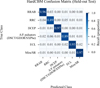 |
Fig. 2 Normalized confusion matrix for HardCBM on the held-out test set (Ntest = 2700). The main confusion occurs between RRC and DSCT/GDOR/SXPhe, consistent with their overlapping period ranges and similar Fourier signatures. Diagonal values represent per-class recall. |
Held-out test set performance with BCa bootstrap 95% CIs.
EndToEndHardCBM concept prediction quality (R2).
4.3 End-to-end CBM results
The EndToEndHardCBM, which learns concept representations from raw phase-folded light curves (Sect. 3.1), achieves 92.9 ± 1.4% accuracy and 87.9 ± 1.8% macro F1 on 2500 balanced sources (5-fold CV). While lower than the x = c HardCBM (94.4%), this model demonstrates a genuine CBM where the concept predictor is learned rather than an identity function.
Table 6 reports concept prediction quality measured by R2 between predicted and true concept values. Photometric concepts (GBP - GRP: R2 = 0.97; mean G: R2 = 0.94) and period (R2 = 0.83) are learned accurately from light curves alone. Fourier ratios and phase differences are harder to extract (R2 = 0.04–0.45), and rise_fraction is essentially unlearnable (R2 < 0). These quality scores indicate which concepts can be reliably inferred from photometric time series and which require catalog-level information.
Crucially, concept intervention in the EndToEndHardCBM setting is genuinely nontrivial. Under σ = 1.0 noise injection into predicted concepts, EndToEndHardCBM accuracy degrades from 92.9% to 52.7 ± 3.4%. Replacing all corrupted concepts with ground truth values recovers accuracy to only 68.5 ± 3.5% – a 73.7% recovery rate, far below the 100% trivially achieved in the x = c setting. This incomplete recovery demonstrates that the concept encoder learns a transformed internal representation that diverges from physical ground truth (consistent with the R2 values in Table 6); the label predictor expects the encoder’s learned distribution, not raw physical values. Per-concept intervention at σ = 1.0 shows GBP - GRP (+1.8 pp), skewness (+1.0 pp), and amplitude (+1.1 pp) as the highest-value correction targets - a different ranking from that obtained in the x = c setting (R31, period, period_snr), reflecting the encoder’s transformation of concept space.
4.4 Accuracy–interpretability trade-off spectrum
The eight models span a continuous accuracy–interpretability spectrum: from XGBoost (99.8%, opaque) through SoftCBM (99.1%, partially interpretable) and HardCBM-Cal (97.0%, moderate) to HardCBM (94.4%, fully interpretable). Only MLP is Pareto-dominated (less accurate than HardCBM-Cal and less interpretable than HardCBM). Practitioners can choose their preferred operating point: HardCBM-Cal when partial concept access suffices, HardCBM when every prediction must be auditable.
4.5 Concept ablation analysis
4.5.1 Single-concept removal (leave-one-out)
Leave-one-out (LOO) ablation (experiment A2b) identifies three concepts whose removal significantly degrades HardCBM accuracy (paired t-test across five folds): R31 (−1.95 ± 0.83 pp, p = 0.006), period_snr (−1.28 ± 0.30 pp, p < 10−3), and skewness (−0.88 ± 0.57pp, p = 0.026). After Bonferroni correction for 12 concepts (α/ 12 = 0.0042), period_snr remains significant and R31 is borderline. The remaining nine concepts show |Δacc| ≲ 0.35 pp with p > 0.10.
However, R31’s importance is partly confounded by the imputation pattern: R21, R31, φ21 are NaN for 50% of sources (nonpulsating classes) and filled with per-class constants, so R31 partly encodes a binary “has Fourier tables” signal. To disentangle this, we performed two complementary tests. First, we repeated the ablation on pulsators only (RRAB + RRC + DCEP, N = 9,000; all genuine Fourier values). The ranking changes substantially: period becomes rank 1 (−6.58 ± 0.57 pp, p < 10−4), R31 takes rank 2 (−2.78 ± 0.59 pp, p < 10−3), and the other ten concepts collapse to |Δ| < 0.4 pp with no single-concept significance. The pulsator-vs-full ranking correlation is moderate (τ = 0.45, p = 0.045): R31 and period anchor both rankings, but concepts that rely on class contrast (e.g., skewness and period_snr, which rank high in the full six-class setting) lose their discriminating role once the nonpulsator classes are removed, while pulsator-specific concepts (e.g., φ21) become visible. Second, we quantified the magnitude of the imputation confound by replacing the constant per-class medians of R21, R31, and φ21 for nonpulsator rows with random draws from the pulsator marginal distribution (Sect. 6.1, F1). Taken together, the two tests show that R31 carries genuine Fourier information (consistent with RR Lyrae Fourier taxonomy (Jurcsik & Kovács 1996) and with the period– luminosity framework (Madore & Freedman 1991)) and that its rank-1 position in the full six-class setting partly reflects the imputation-encoded “has Fourier tables” signal, while period is the underlying physical discriminator within the pulsator family.
4.5.2 Concept group removal and forward selection
Greedy forward selection (experiment A7) reveals that seven concepts achieve 99.6% of full-model performance (93.97% vs. 94.36% with all 12). The optimal ordering is: (1) period, (2) amplitude, (3) skewness, (4) R21, (5) R31, (6) mean_mag, (7) period_snr. The remaining five concepts (φ21, color, kurtosis, rise_fraction, Stetson K) contribute minimal marginal accuracy. In particular, rise_fraction contributes no independent information: It is 100% NaN in Gaia DR3 and collapses to the imputation fallback of 0 (see Table 2 footnote a), producing a zero-variance column that the CBM’s label predictor can only pass through unchanged.
4.6 Concept importance consensus
We assessed concept importance using five independent methods (experiment B3): LOO accuracy drop, ANOVA F -statistic (validated with Levene’s test; Kruskal–Wallis as nonparametric alternative), mutual information, weight norms, and noise sensitivity. R31 and period consistently rank in the top three across all methods (Figure 3). The median pairwise Kendall τ between methods is 0.44, reflecting complementary importance perspectives; the key conclusion – core concepts (period, R31, period_snr) are consistently highly ranked – is robust regardless of methodology. R31 ’s importance partly reflects the Fourier imputation pattern (Sect. 4.5).
5 Concept intervention
The defining advantage of CBMs over black-box models is the ability to intervene (Koh et al. 2020): an expert can inspect and correct individual concept values, immediately observing the effect on classification. We designed a comprehensive intervention experiment (B1) to quantify this capability.
5.1 Noise injection and single-concept recovery
We injected Gaussian noise of varying severity (σ ∈ {0.5, 1.0, 2.0}, applied to standardized concept values) into all 12 concepts simultaneously, then recovered each concept individually by replacing its noisy value with the clean ground truth.
We note that in the x = c setting, a per-concept recovery curve is mathematically equivalent to an inverted single-feature perturbation curve: Corrupting all inputs and then restoring one is the mirror of perturbing one input from the clean state. The distinction is operational rather than mathematical. A standard sensitivity analysis on a feature-based classifier reports how much accuracy drops when each feature is perturbed. The intervention framing reports how much accuracy is repaired when each concept is corrected, directly answering the astronomer workflow question of which single observable should be measured or re-derived when given finite expert attention. This is a forward, actionable protocol rather than a post-hoc attribution. In the EndToEndHardCBM setting, the two are no longer equivalent because g ≠ id (Sect. 4.3); the x = c results therefore establish the ranking property of the intervention mechanism, which is then exercised nontrivially in the end-to-end variant.
Aggregating across all 5 folds, at σ = 1.0, corrupting all concepts degrades HardCBM accuracy from 94.18 ± 0.53% to 62.6 ± 1.0%. Recovering concepts one at a time reveals their individual contributions (Figure 4):
R31: largest single-concept recovery (+7.3 pp).
period: second largest (+2.9 pp).
period_snr: third (+2.6 pp).
Recovering all concepts restores accuracy to the original 94.18% (100% recovery rate at all noise levels), as expected in the x = c setting where restoring concepts restores inputs (Sect. 3.1). The true value of the intervention mechanism is the structured interface: the concept layer tells a domain expert exactly which physical quantity to inspect and correct, enabling targeted, scientifically meaningful corrections.
5.2 Misclassification diagnosis: A CBM case study
To demonstrate CBM’s diagnostic value beyond aggregate statistics, we analyzed the 157 misclassified sources (5.1% error rate) on the held-out test set. We classified each misclassification by whether correcting abnormal concept values (>2σ from the true-class mean) changes the prediction:
Concept-correctable (58 sources, 37%): correcting 1–2 concept values fixes the prediction. For example, an RRC source misclassified as RRAB has R31 at + 13.1σ from the RRC mean; replacing R31 with the class mean immediately corrects the prediction. This type of error is directly actionable by domain experts.
Boundary cases (85 sources, 54%): the source lies near class decision boundaries with no single concept correction sufficing.
Systematic (14 sources, 9%): the concept profile genuinely matches the predicted (wrong) class, suggesting possible label noise or physically ambiguous objects.
In deployment, an astronomer observing an outlier concept value (>2σ from any class mean) can flag the source, verify the corresponding observable, and correct it if erroneous. The concept most frequently involved in corrections is R31, followed by period and period_snr. This structured error diagnosis is natively provided by the CBM bottleneck without additional post-hoc computation.
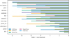 |
Fig. 3 Concept importance consensus across five independent methods. Bars show per-method rank (1 = most important) for each of the 12 concepts, sorted by mean rank. R31 and period consistently rank highest across all methods. The moderate cross-method agreement (median Kendall τ = 0.44) reflects complementary importance perspectives. |
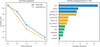 |
Fig. 4 Concept intervention analysis (5-fold aggregate). Left: Accuracy degradation under increasing Gaussian noise (σ) for HardCBM. Right: Per-concept accuracy recovery at σ = 1.0 when each concept is individually corrected. R31 yields the largest single-concept recovery (+7.3 pp), followed by period (+2.9 pp) and period_snr (+2.6 pp). This per-concept sensitivity ranking is the primary finding of the intervention experiment. |
5.3 Comparison with black-box baselines
At σ = 1.0, RF drops from 99.85% to 30.6% (−69.2pp) with no repair mechanism, versus HardCBM’s −32.6 pp with perconcept recovery. This asymmetry – repairable degradation vs. catastrophic failure – is the core argument for CBMs in scientific applications.
5.4 Brightness-stratified analysis
Fainter sources in Gaia have fewer photometric epochs and larger measurement uncertainties, creating a natural gradient of data quality. We evaluated models on three magnitude bins (experiment B6): bright (G < 14, N = 567), medium (14 ≤ G < 17, N = 997), and faint (G ≥ 17, N = 1,136).
Fourier concepts show the largest variance increase in faint sources (R21 3.18×, R31 2.83×), making them the highest-priority intervention targets for faint-source catalogs. The same concepts also exhibit the largest cross-survey shift (Sect. 6.3), so their catalog values warrant verification against the underlying light curve before they are relied upon in the faint regime.
6 Discussion
6.1 Astronomical insights
Our experiments yield seven physical findings (B10): (F1) R31 ’s rank-1 importance in the full six-class problem is partly an imputation artifact; pulsator-only ablation promotes period to rank 1 (Sect. 4.5). Replacing the constant per-class median imputation of R21, R31, and φ21 for nonpulsator rows with random draws from the pulsator marginal distribution – so that the imputation itself no longer encodes a binary “has Fourier” signal – reduces overall HardCBM accuracy from 94.29 ± 0.59% to 93.20 ± 0.55% (a paired decrease of 1.09 pp, Nadeau-Bengio corrected paired t-test p = 0.002 on per-fold differences), while the perfold R31 LOO drop (matched 5-fold seed and splits) moves from 1.95 ± 0.83 pp to 2.17 ± 0.36 pp - a change of +0.22pp that is not statistically distinguishable from zero (paired t-test p = 0.38; Wilcoxon signed-rank p = 0.44). The full R31 LOO therefore survives destruction of the imputation signal, consistent with R31 carrying genuine Fourier information; the significant drop in full-model accuracy confirms, equally honestly, that the imputation pattern was contributing a small but nonzero classification signal in the standard setting. (F2) The Fourier group is the most critical concept group (Debosscher et al. 2007; Richards et al. 2011), though Fourier parameters lack direct physical meaning for eclipsing binaries (Sect. 6.6). (F3) The period-color correlation (r = 0.66) reflects period-luminositycolor relations (Madore & Freedman 1991). (F4) rise_fraction is 100% NaN in Gaia DR3 and collapses to the imputation fallback of 0; as a zero-variance input it carries no classification signal and is eliminated first in backward selection (with essentially no accuracy loss), confirming the pipeline’s expectation that this concept is unavailable without raw epoch photometry. (F5) period_snr has the lowest variance inflation factor (VIF; 1.12), carrying information orthogonal to all physical concepts. (F6) Fourier parameters show the largest variance increase in faint sources (Sect. 5.4). (F7) Seven concepts retain 99.6% of performance, spanning 4/5 physical groups.
6.2 Comparison with Gaia DR3 pipeline
Direct numerical comparison with Rimoldini et al. (2023) is not straightforward: They classify 25 types using ~50 features on the full catalog, while we classify six types with 12 concepts on a balanced subset. Rimoldini et al. (2023) report recall of 70.0% (RR Lyrae), 75.2% (Cepheids), and 47.8% (ECL); per-class F1 for the corresponding classes in our HardCBM is 87.1% (RRAB)/97.3% (RRC), 86.2% (DCEP), and 97.8% (ECL). Because precision is high in our balanced setting, these F1 values are close to but not identical to recall and are substantially higher than Rimoldini’s recall in all cases. This gap should be read with three caveats: (i) Our six-class problem is easier than Rimoldini’s 25-class problem because several fine-grained types we exclude (e.g., RRd, T2CEP, ACEP) are the same ones where their classifier struggles; (ii) balanced sampling eliminates the class-imbalance headwind their pipeline faces; (iii) ground truth is derived from the same curated catalogs, so the problems are not strictly independent. Our contribution is therefore not that HardCBM beats Rimoldini’s pipeline on raw accuracy (it cannot on the same 25-class task) but that HardCBM delivers comparable or better recall on a six-class subproblem while exposing the per-prediction traceability through 12 named physical quantities that the Rimoldini pipeline does not.
Comparison with light-curve deep-learning classifiers. Deeplearning models operating directly on light curves – recurrent neural network (RNN)-based classifiers (Naul et al. 2018) and recurrent networks with metadata fusion (Jamal & Bloom 2020) – report accuracies in the range 88–99% depending on class scheme, survey, and sample size. HardCBM’s balanced 94.4% and prior-weighted 98.2% lie within this range, while providing a qualitatively different capability: The predictions are constrained to flow through a layer of 12 named physical quantities, whereas the RNN-based classifiers expose only light-curve-time representations that require post-hoc methods to interpret. The End-ToEndHardCBM variant (Sect. 4.3) closes the methodological gap to these works by learning concepts from raw photometry; its 92.9% on 2500 sources already matches the lower end of the deep-learning band while inheriting the CBM’s forward intervention interface. Scaling EndToEndHardCBM to the full 18 000-source (and ultimately Gaia DR4) regime is the most direct extension of the present work (Sect. 6.6, Tier 1).
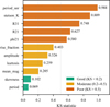 |
Fig. 5 Domain shift between Gaia and OGLE concept distributions quantified by KS statistics. Concepts derived from survey-specific processing (period_snr, Stetson K) show the most severe shift (KS > 0.8, red), while band-independent concepts (period, skewness) transfer well (KS < 0.2, green). The CBM concept layer enables this per-concept diagnosis, which is impossible with black-box models. |
6.3 Cross-survey generalization
Evaluating Gaia-trained models on OGLE data (experiment B8) reveals severe domain shift. Zero-shot accuracy is 17.5% for HardCBM (near the 16.7% random baseline) and 43.8% for RF (Ntest = 240). HardCBM collapses to a single-class (RRC) predictor – itself a diagnostic signal that domain-shifted concept values cluster in one region of concept space.
Kolmogorov–Smirnov (KS) tests between Gaia and OGLE concept distributions (Figure 5) reveal three concepts with extreme shift (KS > 0.7): period_snr (0.99), Stetson K (0.89), and R31 (0.75) – precisely the concepts most affected by surveyspecific processing differences. The extreme period_snr shift in particular follows from its differing definition in the two pipelines (Sect. 6.6), whereas the Stetson K and R31 shifts reflect band-dependent sampling and Fourier extraction.
After fine-tuning on 60% of OGLE data (learning rate 10−4, patience 10, max. 100 epochs, all layers unfrozen), RF recovers to 96.3% while HardCBM reaches only 53.3%. The bottleneck simultaneously provides diagnostic value (per-concept shift detection) and limits adaptation capacity. Period transfers well (KS = 0.069), but Fourier ratios show substantial shift (R21 KS = 0.627, R31 KS = 0.748), likely reflecting pipeline differences.
Targeted concept recalibration (replacing the three highest-KS concepts with OGLE-derived values) does not recover performance (∼17%), nor does oracle replacement of all 12 concepts with per-class OGLE medians – indicating that the joint concept distribution, not individual marginals, must be realigned. These results demonstrate that while CBMs can directly diagnose which concepts fail to transfer through their explicit intermediate layer, effective cross-survey adaptation requires model fine-tuning rather than concept substitution.
6.4 The accuracy–interpretability trade-off
The 5.4 pp accuracy gap between HardCBM and XGBoost buys an architectural property that the RF cannot offer: every prediction is traceable through the 12 named quantities, an astronomer can correct an individual concept value and immediately read the effect on the class posterior, and when the model fails on new survey data the concept layer points directly to which physical quantities have shifted. Since RF uses the same 12 features, the entire gap is attributable to this bottleneck constraint.
Relationship to post-hoc attribution (SHAP). A natural question is whether the CBM’s advantages can be recovered by applying SHAP (Lundberg & Lee 2017) to a random forest operating on the same 12 named features. Table 3 summarizes the comparison. SHAP on RF delivers per-prediction attribution to the same named features at 99.8% accuracy, so when the use case is explaining an individual decision after the fact, the practical gap relative to HardCBM’s 94.4% is small and in fact favors SHAP+RF. What SHAP cannot provide is: (a) an architectural guarantee that the model did not exploit interactions outside the named features – the RF is free to base its predictions on combinations that only acquire meaning through the SHAP explanation itself; (b) a forward intervention API, where an astronomer assigns a corrected value to a named concept and reads the updated class posterior in a single forward pass without re-invoking an attribution algorithm; and (c) a mechanism for per-concept cross-survey domain-shift diagnosis, which relies on the concept layer existing as an explicit intermediate representation rather than a post-hoc lens over an opaque one. In the EndToEndHardCBM setting, a further nontrivial gap opens, because the CBM’s learned concept layer has no post-hoc analogue: SHAP values on raw light-curve inputs would attribute decisions to phase bins rather than to physical quantities.
Empirically, SHAP global importance on RF correlates only weakly to moderately with CBM LOO importance (τ = 0.27, p = 0.25 on the corrected dataset), indicating that the two lenses disagree substantially on individual concept rankings (e.g., SHAP ranks period first and R31 second, whereas CBM LOO ranks R31 first and period outside the top three), even though both methods identify a similar set of concepts in the upper half of the ordering. We therefore regard SHAP+RF as the appropriate tool when maximum accuracy and retrospective explanation are the priorities; CBMs are preferable when intrinsic transparency, forward intervention, and structured concept-level domain diagnostics are required (Rudin 2019).
6.5 Guidance for practitioners
The end-to-end concept R2 values in Table 6, together with the brightness-stratified variance increase in Sect. 5.4, let us sort the 12 concepts by how safely they can be used as intermediate interpretable quantities in a Gaia-based workflow. We offer the following pragmatic guidance for future users of CBM-like pipelines.
Group I – catalog stable, inspection ready. period, GBP - GRP, mean G, and amplitude transfer almost losslessly from raw light curves (end-to-end R2 ≥ 0.67), remain stable across the Gaia magnitude range (Table 7), and match the corresponding OGLE marginals (KS < 0.2; Sect. 6.3). Astronomers can treat these as trustworthy concepts: intervention on these concepts carries a clear observational analogue and the CBM’s per-concept coefficient can be compared directly with astrophysical expectation (e.g., period–luminosity relations).
Group II – use with survey-specific caveats. R21, R31, φ21, skewness, kurtosis, and Stetson K carry genuine discriminating power (they dominate the LOO importance ranking; Sect. 4.5) but are survey-specific in two ways: (i) their end-to-end R2 values are moderate (0.25–0.45, excluding φ21), meaning that recovering them from raw photometry requires enough epochs that a Fourier fit is well-posed; and (ii) they show the largest brightness-dependent variance inflation and the largest crosssurvey KS statistics. When applying a CBM trained on Gaia to another survey, these are the concepts most in need of recalibration; when intervening on them, astronomers should couple the correction with a check on the supporting light curve rather than accepting the catalog value directly.
Group III – Gaia-only or deferred. rise_fraction is unavailable in the Gaia catalog pipeline (100% NaN) and essentially unlearnable from 100-bin phase-folded Gaia light curves (R2 < 0). period_snr is available, but its definition diverges between the light-curve pipeline (- log10 FAP) and the catalog pipeline (2 log10(period/σP)), producing the extreme cross-survey shift of Sect. 6.3. Practitioners deploying a Gaia-trained CBM on a non-Gaia survey should either re-derive period_snr in a common definition or down-weight its intervention value. Where survey coverage permits (e.g., OGLE dense-cadence I-band), computing rise_fraction and period_snr directly from the light curve is always preferable to catalog imputation.
The groups above summarize the concept-recovery and domain-shift experiments in the form most useful when deploying a CBM on a new survey. They also explain why the nontrivial per-concept recovery ranking (Sect. 5.1) matches group structure: Group I concepts contribute smaller recovery gains because they are harder to corrupt in practice, while Group II concepts (led by R31) dominate recovery because they are both discriminating and easiest to corrupt through sampling or survey-translation effects.
Performance by brightness (held-out test set).
6.6 Limitations
Our work has several limitations:
Precomputed concepts (x = c; Sect. 3.1): This renders certain CBM properties tautological – concept extraction is perfect by construction, full-concept intervention trivially recovers the input (Sect. 5.1), and rise_fraction is unavailable (100% NaN) because it cannot be derived from Gaia catalog statistics alone. The limitation is therefore on the scope of claims rather than on the concept-constrained classifier framework itself: the x = c experiments validate the intervention ranking, the architectural guarantee, and the concept-level domain-shift diagnostic, but they cannot validate concept learning quality. The EndToEndHardCBM prototype (Sect. 4.3) exercises the remaining nontrivial properties, but on a smaller sample (2500 sources) limited by epoch-photometry availability. Scaling the end-to-end setting to the full 18 000-source dataset – and ultimately to Gaia DR4 – is the most important next step (see “Priority for future work” below).
Six classes: We classified six variability types; the Gaia pipeline handles 25. Extending to more classes may require additional concepts. Our simplified scheme is not a production classifier but a demonstration of the CBM framework’s capabilities.
Physically heterogeneous classes: DSCT/GDOR/SXPhe merges δ Scuti ( p-mode), γ Doradus (g-mode), and SX Phe (Pop. II) stars; a kernel density estimate (KDE) of the period distribution confirms three distinct peaks (Ashman D = 2.9). MIRA/SR spans Mira, semi-regular, and OSARG stars over two orders of magnitude in amplitude, producing high internal class diversity.
Fourier parameters for eclipsing binaries: R21, R31, φ21 describe pulsation harmonics and lack direct physical meaning for ECL, where light curve shape is governed by Roche-lobe geometry.
Eclipsing binary half-period aliasing: Automated periodfinding may recover half the true orbital period for ECL (Rimoldini et al. 2023); our pipeline adopted catalog periods without correction.
Amplitude definition: The light-curve pipeline uses P98 - P2 (percentile proxy), while the Gaia catalog uses class-specific columns (peak_to_peak_g, amplitude_estimate, geom_model_gaussian1_depth). This nonuniform definition may contribute to cross-survey domain shift.
Stetson K index: We used the single-band version (Stetson 1996), not the original two-band formulation.
Fourier parameter imputation: R21, R31, and φ21 are NaN for 50% of sources (nonpulsating classes) and are filled with per-class median constants, effectively encoding a binary “Fourier-available” signal. Our randomization test (Sect. 6.1, F1) quantifies the magnitude of this confound: when the constant medians are replaced by random draws from the pulsator marginal distribution, overall HardCBM accuracy decreases by 1.1 pp – so the imputation pattern was contributing a small but nonzero classification signal – while R31 ’s LOO importance is statistically unchanged at ∼ 2pp (standard 1.95 pp, randomized 2.17 pp). Three avenues could in principle remove this confound more cleanly than median imputation. First, adding an explicit “Fourier-available” binary concept would move the implicit signal into a named scalar and let the CBM account for it without conflating it with R31 . Second, model-based imputation – e.g., a tabular foundation model (Hollmann et al. 2023) conditioned on the other (non-Fourier) concepts – could produce context-aware fill values rather than constants; the caveat is that a nonpulsator has no physical Fourier harmonic structure to recover, so any imputed value is by construction synthetic rather than inferred from the underlying astrophysics. Third, and in our view preferably, computing R21, R31, and φ21 directly from raw Gaia epoch photometry for nonpul-sator classes would produce physically meaningful values (harmonic ratios of whatever light-curve shape the source actually exhibits) and would make the “has Fourier tables” signal redundant with Gaia’s processing history rather than with astrophysics. This last option is aligned with the Tier 1 priority below (end-to-end concept learning).
Definition of period_snr: The feature extraction pipeline computes - log10(FAP); the Gaia catalog uses 2 log10(period/σP). These fundamentally different quantities contribute to the extreme KS statistic (= 0.988) for period_snr in cross-survey comparisons (Sect. 6.3).
Cross-survey transfer: HardCBM’s fine-tuning recovery (53.3%) trails RF (96.3%; Sect. 6.3).
Concept selection: While our 12 concepts are grounded in literature, the selection process involves expert judgment. Future work could explore automatic concept discovery.
Brightness-biased sampling: Our brightest-3 000 downsampling does not inflate accuracy (S2/S3: leave-bright-out 97.1% vs. full 94.7%), but remains nonrepresentative of the full Gaia magnitude distribution.
Sample size: Our 18 000-source dataset (learning curve plateaus near 10 000 samples) is a small fraction of Gaia’s 12.4 million variable candidates.
Priority for future work. The 13 limitations above are not equally urgent. In our view they fall into four tiers.
Tier 1 (address first), end-to-end concept learning at scale. Limitation 1 (x = c) is the single constraint that determines how many CBM-specific claims this paper can validate. The End-ToEndHardCBM prototype (Sect. 4.3) shows the technical path, but at 2500 sources it cannot be compared like-for-like with the 18 000-source precomputed experiments. Scaling the end-to-end variant to the full dataset, and then to Gaia DR4’s deeper epoch photometry, directly converts several currently trivial properties (concept-R2 reporting, nontrivial intervention recovery, genuine concept-level domain adaptation) into measurable quantities. This tier subsumes limitation 13 as its scaling target.
Tier 2 (address second), disentangling Fourier imputation from physics. Limitation 8 (Fourier imputation) inflates R31 ’s apparent importance and partially confounds the leave-one-out ranking. The pulsator-only ablation (Sect. 4.5) and the Fourier-randomization experiment described below already bracket the effect, but a principled future treatment would add an explicit “has Fourier” binary concept, use class-neutral imputation, or – best of all – derive the Fourier harmonics from raw Gaia DR3/DR4 epoch photometry for nonpulsating classes rather than imputing them.
Tier 3 (address with expanded data), taxonomy completeness and class heterogeneity. Limitations 2 and 3 are structural: moving to Gaia’s 25-type taxonomy and splitting the merged DSCT/GDOR/SXPhe and MIRA/SR classes will probably require additional concepts (mode-type indicators, spectral-class proxies) beyond the 12 used here, plus targeted sampling for the statistically weaker classes (T2CEP, ACEP, RRd, RRe).
Tier 4 (engineering consolidation), definition unification and cross-survey adaptation. Limitations 6, 7, 9 (amplitude, Stetson K, period_snr definitions) and 5 (ECL half-period aliasing) are well-understood pipeline-level issues that a production deployment must fix but that do not change the scientific conclusions of this work. Limitation 10 (cross-survey transfer) is higher-science but depends on Tier 1 and Tier 4: meaningful concept-space domain adaptation needs both a learned g and unified concept definitions.
We therefore regard Tier 1 as the single most important next step and the one whose completion would most strongly extend the validity of the results reported here. The remaining tiers refine and broaden the framework but do not alter the core scientific conclusions of this work.
7 Conclusion
We have presented, to our knowledge, the first peer-reviewed application of concept bottleneck models to astronomical source classification, demonstrating that variable star classification can be performed through physically meaningful intermediate concepts rather than opaque feature transformations. Our key findings are:
CBMs are viable for astronomical classification: HardCBM achieves 94.4% accuracy on a balanced six-class variable star dataset. The 5.4 pp gap relative to random forest is the cost of an architectural guarantee that the model operates only through 12 named physical quantities, preventing nonphysical shortcuts and ensuring every prediction is fully traceable.
Concept intervention provides structured diagnostics: The nontrivial finding is the per-concept sensitivity ranking (R31 > period > period_snr), which identifies which concepts are highest-value correction targets and in what order – information unavailable from a black-box model. Under σ = 1.0 noise, HardCBM recovers from 62.6% to 94.2% (five-fold aggregate; expected in the x = c setting), while RF collapses from 99.85% to 30.6% with no repair mechanism. In the EndToEndHardCBM setting, recovery reaches only 73.7%, confirming that learned concept representations diverge from physical ground truth (Sect. 4.3).
Physical insights require imputation-aware analysis: R31 ranks first overall, but pulsator-only ablation promotes period to rank 1, and a randomization test confirms that R31 ’s LOO importance (∼2 pp) is genuine Fourier physics (unchanged after the per-class imputation signal is broken) while the imputation pattern contributes 1.1 pp of spurious overall accuracy (Sect. 4.5). Seven concepts retain 99.6% of classification performance.
CBMs diagnose domain shift: cross-survey evaluation reveals that the concept layer can pinpoint which specific concepts fail to transfer, enabling targeted diagnosis of concept-level domain shift, although naive concept replacement alone proves insufficient for performance recovery (Sect. 6.3).
End-to-end concept learning is feasible: our EndToEndHard-CBM learns concepts from raw phase-folded light curves, achieving 92.9% accuracy while producing inspectable concept predictions with R2 up to 0.97 for photometric concepts.
These results are demonstrated on a brightness-biased sample; scaling the EndToEndHardCBM to the full dataset is the most important next step. We expect the denser phase coverage of Gaia DR4 to further improve the learned concept representations and to narrow the gap to the precomputed setting.
Outlook: Deployment on forthcoming surveys. The methodology developed here is designed to scale to the next generation of time-domain surveys. Gaia DR4 (Gaia Collaboration 2016), expected within the scope of this paper’s publication window, will deliver approximately 5.5 years of epoch photometry – more than double the ∼22-month DR3 baseline used in this work – with correspondingly denser phase coverage and improved Fourier-parameter recovery; we expect DR4 to be the natural setting in which to retire the x = c simplification and train EndToEndHardCBM end-to-end on a 106-source scale. The upcoming Vera C. Rubin Observatory LSST (Ivezic´ et al. 2019), with its 10-year, multi-band, ∼109 -alert stream, will require precisely the per-concept cross-survey domain-shift diagnosis we demonstrate in Sect. 6.3, since no training set will be both representative and large enough to be survey-agnostic. Ongoing alert-broker surveys, such as that from the Zwicky Transient Facility (Chen et al. 2020), are a natural testbed for online deployment. Our Gaia→OGLE experiments (17.5% zero-shot, 53.3% fine-tuned vs. RF’s 96.3%) are a cautionary benchmark: substantial advances in concept-space domain adaptation – probably combining survey-conditional calibration layers, unified concept-definition pipelines, and direct Fourier recovery from raw photometry – are needed before a single CBM can operate across surveys without retraining. The EndToEndHard-CBM demonstrates that concept extraction from raw photometry is feasible; it provides the architectural foundation on which those survey-agnostic CBM pipelines can be built.
Acknowledgements
This work has made use of data from the European Space Agency (ESA) mission Gaia (https://www.cosmos.esa.int/gaia), processed by the Gaia Data Processing and Analysis Consortium (DPAC; https://www.cosmos.esa.int/web/gaia/dpac/consortium). This research also made use of the OGLE Collection of Variable Stars. We acknowledge the use of PyTorch (Paszke et al. 2019), scikit-learn (Pedregosa et al. 2011), and XGBoost (Chen & Guestrin 2016).
Data availability
The Gaia DR3 data used in this work are publicly available through the Gaia Archive3, and the OGLE-IV data are available from the OGLE Collection of Variable Stars4. The supplementary datasets generated for this study are deposited in a public Zenodo archive at https://doi.org/10.5281/zenodo.20571389. The archive provides the per-class AUC-ROC scores for all eight models, the Holm–Bonferroni-corrected significance tests, the accuracy–interpretability Pareto frontier, the 12-concept correlation matrix (with variance inflation factors), and the cross-survey Kolmogorov–Smirnov statistics, together with the processed concept feature matrices and the trained model checkpoints. The full source code for data processing, model training, and all experiments – including the per-fold imputation, evaluation metrics, and statistical-testing infrastructure – is included in the same archive.
References
- Benavoli, A., Corani, G., Demšar, J., & Zaffalon, M. 2017, JMLR, 18, 1 [Google Scholar]
- Breiman, L. 2001, Mach. Learn., 45, 5 [Google Scholar]
- Chen, T., & Guestrin, C. 2016, in Proceedings of the 22nd ACM SIGKDD International Conference on Knowledge Discovery and Data Mining, 785 [Google Scholar]
- Chen, X., Wang, S., Deng, L., et al. 2020, ApJS, 249, 18 [NASA ADS] [CrossRef] [Google Scholar]
- Clementini, G., Ripepi, V., Garofalo, A., et al. 2023, A&A, 674, A18 [NASA ADS] [CrossRef] [EDP Sciences] [Google Scholar]
- Cohen, J. 1960, Educ. Psychol. Meas., 20, 37 [CrossRef] [Google Scholar]
- Deb, S., & Singh, H. P. 2009, A&A, 507, 1729 [NASA ADS] [CrossRef] [EDP Sciences] [Google Scholar]
- Debosscher, J., Sarro, L. M., Aerts, C., et al. 2007, A&A, 475, 1159 [NASA ADS] [CrossRef] [EDP Sciences] [Google Scholar]
- Efron, B. 1987, J. Am. Stat. Assoc., 82, 171 [Google Scholar]
- Eyer, L., & Mowlavi, N. 2008, in Journal of Physics Conference Series, 118, 012010 [Google Scholar]
- Eyer, L., Audard, M., Holl, B., et al. 2023, A&A, 674, A13 [NASA ADS] [CrossRef] [EDP Sciences] [Google Scholar]
- Gaia Collaboration (Prusti, T., et al.) 2016, A&A, 595, A1 [NASA ADS] [CrossRef] [EDP Sciences] [Google Scholar]
- Gaia Collaboration (Vallenari, A., et al.) 2023, A&A, 674, A1 [NASA ADS] [CrossRef] [EDP Sciences] [Google Scholar]
- Havasi, M., Parbhoo, S., & Doshi-Velez, F. 2022, in Advances in Neural Information Processing Systems, 35, 23386 [Google Scholar]
- Hollmann, N., Müller, S., Eggensperger, K., & Hutter, F. 2023, in International Conference on Learning Representations (ICLR) [Google Scholar]
- Holm, S. 1979, Scand. J. Stat., 6, 65 [Google Scholar]
- Ivezic´, Ž., Kahn, S. M., Tyson, J. A., et al. 2019, ApJ, 873, 111 [NASA ADS] [CrossRef] [Google Scholar]
- Jamal, S., & Bloom, J. S. 2020, ApJS, 250, 30 [NASA ADS] [CrossRef] [Google Scholar]
- Jurcsik, J., & Kovács, G. 1996, A&A, 312, 111 [NASA ADS] [Google Scholar]
- Kim, D.-W., & Bailer-Jones, C. A. L. 2016, A&A, 587, A18 [NASA ADS] [CrossRef] [EDP Sciences] [Google Scholar]
- Koh, P. W., Nguyen, T., Tang, Y. S., et al. 2020, in Proceedings of the 37th International Conference on Machine Learning, 119 (PMLR), 5338 [Google Scholar]
- Lebzelter, T., Mowlavi, N., Marrese, P. M., et al. 2023, A&A, 674, A15 [NASA ADS] [CrossRef] [EDP Sciences] [Google Scholar]
- Lieu, M. 2025, Universe, 11, 187 [Google Scholar]
- Lomb, N. R. 1976, Ap&SS, 39, 447 [Google Scholar]
- Loshchilov, I., & Hutter, F. 2019, in International Conference on Learning Representations [Google Scholar]
- Lundberg, S. M., & Lee, S.-I. 2017, NeurIPS, 30, 4766 [Google Scholar]
- Madore, B. F., & Freedman, W. L. 1991, PASP, 103, 933 [Google Scholar]
- Matthews, B. W. 1975, Biochim. Biophys. Acta, 405, 442 [Google Scholar]
- McNemar, Q. 1947, Psychometrika, 12, 153 [Google Scholar]
- Mowlavi, N., Holl, B., Lecoeur-Taïbi, I., et al. 2023, A&A, 674, A16 [NASA ADS] [CrossRef] [EDP Sciences] [Google Scholar]
- Nadeau, C., & Bengio, Y. 2003, Mach. Learn., 52, 239 [Google Scholar]
- Naul, B., Bloom, J. S., Pérez, F., & van der Walt, S. 2018, Nat. Astron., 2, 151 [NASA ADS] [CrossRef] [Google Scholar]
- Oikarinen, T., Das, S., Nguyen, L. M., & Weng, T.-W. 2023, in International Conference on Learning Representations [Google Scholar]
- Pashchenko, I. N., Sokolovsky, K. V., & Gavras, P. 2018, MNRAS, 475, 2326 [NASA ADS] [CrossRef] [Google Scholar]
- Paszke, A., Gross, S., Massa, F., et al. 2019, NeurIPS, 32, 8024 [Google Scholar]
- Pedregosa, F., Varoquaux, G., Gramfort, A., et al. 2011, JMLR, 12, 2825 [Google Scholar]
- Richards, J. W., Starr, D. L., Butler, N. R., et al. 2011, ApJ, 733, 10 [NASA ADS] [CrossRef] [Google Scholar]
- Rimoldini, L., Holl, B., Gavras, P., et al. 2023, A&A, 674, A14 [NASA ADS] [CrossRef] [EDP Sciences] [Google Scholar]
- Ripepi, V., Clementini, G., Molinaro, R., et al. 2023, A&A, 674, A17 [NASA ADS] [CrossRef] [EDP Sciences] [Google Scholar]
- Rudin, C. 2019, Nat. Mach. Intell., 1, 206 [Google Scholar]
- Sánchez-Sáez, P., Reyes, I., Valenzuela, C., et al. 2021, AJ, 161, 141 [CrossRef] [Google Scholar]
- Scargle, J. D. 1982, ApJ, 263, 835 [Google Scholar]
- Simon, N. R., & Lee, A. S. 1981, ApJ, 248, 291 [NASA ADS] [CrossRef] [Google Scholar]
- Soszyński, I., Pawlak, M., Pietrukowicz, P., et al. 2016, Acta Astron., 66, 405 [NASA ADS] [Google Scholar]
- Stetson, P. B. 1996, PASP, 108, 851 [NASA ADS] [CrossRef] [Google Scholar]
- Udalski, A., Szyman´ ski, M. K., & Szyman´ ski, G. 2015, Acta Astron., 65, 1 [NASA ADS] [Google Scholar]
- Yuksekgonul, M., Wang, M., & Zou, J. 2023, in International Conference on Learning Representations [Google Scholar]
- Zarlenga, M. E., Barbiero, P., Ciravegna, G., et al. 2022, in Advances in Neural Information Processing Systems, 35, 21400 [Google Scholar]
Appendix A Per-class concept distributions
Figure A.1 shows the distribution of each of the 12 concepts, stratified by the six variability classes, on the full 18 000-source Gaia DR3 dataset used for cross-validation and testing. Three aspects of the panel are worth highlighting for the discussion of classification confusion (Figure 2) and the imputation-confound analysis (Sect. 4.5, Sect. 6.6):
The Fourier panels (R21, R31, φ21) show visibly narrow, delta-like distributions for the three nonpulsating classes (DSCT/GDOR/SXPhe, ECL, MIRA/SR). These are the per-class median imputations discussed in Sect. 6.6: for these classes the Gaia catalog does not populate the pulsator-specific Fourier tables, and the imputation procedure therefore assigns a single value per class. R21 and R31 distributions for the pulsators (RRAB, RRC, DCEP) retain broad, physically meaningful spreads.
The two most-confused classes in Figure 2—RRC and DSCT/GDOR/SXPhe—exhibit extensively overlapping period, amplitude and Stetson K distributions, which is the primary physical origin of the confusion: their R21 and R31 panels cannot resolve the overlap because the DSCT/GDOR/SXPhe values are imputed constants.
The rise_fraction panel is flat at zero across all classes, reflecting the 100% NaN rate in Gaia DR3 and the nan_to_num fallback described in Table 2. This is the concept that the EndToEndHardCBM encoder also fails to learn (R2 < 0; Table 6) and the one which the backward selection eliminates first (Sect. 4.5).
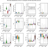 |
Fig. A.1 Per-class distribution of the 12 CBM concepts on the full 18 000-source Gaia DR3 dataset. Shaded vertical bands in the Fourier panels highlight the three nonpulsating classes, whose values are imputed to per-class medians (Sect. 6.6). |
Appendix B Representative light curves and misclassification case studies
Figure B.1 shows one Gaia DR3 phase-folded light curve per class, drawn from the subset of sources for which epoch photometry is available, chosen to exhibit a canonical morphology for that class (RRAB and RRC from vari_rrlyrae, DCEP from vari_cepheid, the remaining three from the general variability tables). For the long-period Mira/SR example the curve is shown in the time rather than phase domain, because the orbital baseline (∼ 1000 d) is only ∼ 2 times the period and phase folding is not stable. Figure B.2 shows three characteristic misclassifications from the held-out test set, one from each of the three categories identified in Sect. 5.2: a concept-correctable RRC→RRAB error driven by an outlier R31 value; a boundary case DCEP→RRAB error with no single fixable concept; and a systematic ECL→DCEP error whose concept profile genuinely matches the predicted (wrong) class. We display these as concept-profile plots rather than as phase-folded light curves for two reasons: none of the 157 held-out misclassifications falls within the 2,500-source EndToEndHardCBM subset for which Gaia epoch photometry was downloaded, and the concept-profile view is in any case a more direct illustration of the three categories—it makes the > 2σ deviation of R31 in case (a), the absence of any single such deviation in case (b), and the matched-to-wrong-class profile in case (c) all immediately legible. Red asterisks mark concepts whose scaled value deviates by more than 2σ from the true-class mean; these are the concepts that an astronomer would prioritise for inspection during the intervention workflow described in Sect. 5.2.
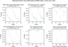 |
Fig. B.1 Representative Gaia DR3 light curves of the six variability classes. Phase-folded using Lomb–Scargle periods estimated from the epoch photometry; the long-period Mira/SR panel is shown in time-domain. Error bars use Gaia per-epoch magnitude uncertainties. |
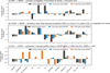 |
Fig. B.2 Three representative misclassified sources from the held-out test set, one per category from Sect. 5.2: (a) a concept-correctable RRC→RRAB error; (b) a boundary case; (c) a systematic case. Bars show the source’s 12 scaled concept values against the mean concept profile of the true class (blue) and the predicted class (orange). Red asterisks flag concepts that deviate by more than 2σ from the true-class mean—these are the actionable intervention targets for an astronomer inspecting the prediction. |
This per-fold imputation is implemented in the main cross-validation pipeline; supplementary ablation experiments use pool-level imputation statistics computed on the full CV pool, introducing a minor information leak whose effect we estimate to be negligible: each training fold retains 80% of the per-class data (∼2040 sources), so per-class medians have a standard error of ≈1.25 σ/√2040, i.e., ∼0.03 σ per concept – an input perturbation far smaller than the ±0.3% CV standard deviation of accuracy, upper-bounding the metric bias at well below 0.1%.
All Tables
All Figures
|
Fig. 1 Concept bottleneck model architecture for variable star classification. Input features pass through a 12-dimensional concept bottleneck of named physical quantities before reaching the label predictor. The concept layer enables expert intervention: astronomers can inspect and correct individual concept values (dashed arrow) to immediately observe the effect on classification. |
| In the text | |
|
Fig. 2 Normalized confusion matrix for HardCBM on the held-out test set (Ntest = 2700). The main confusion occurs between RRC and DSCT/GDOR/SXPhe, consistent with their overlapping period ranges and similar Fourier signatures. Diagonal values represent per-class recall. |
| In the text | |
|
Fig. 3 Concept importance consensus across five independent methods. Bars show per-method rank (1 = most important) for each of the 12 concepts, sorted by mean rank. R31 and period consistently rank highest across all methods. The moderate cross-method agreement (median Kendall τ = 0.44) reflects complementary importance perspectives. |
| In the text | |
|
Fig. 4 Concept intervention analysis (5-fold aggregate). Left: Accuracy degradation under increasing Gaussian noise (σ) for HardCBM. Right: Per-concept accuracy recovery at σ = 1.0 when each concept is individually corrected. R31 yields the largest single-concept recovery (+7.3 pp), followed by period (+2.9 pp) and period_snr (+2.6 pp). This per-concept sensitivity ranking is the primary finding of the intervention experiment. |
| In the text | |
|
Fig. 5 Domain shift between Gaia and OGLE concept distributions quantified by KS statistics. Concepts derived from survey-specific processing (period_snr, Stetson K) show the most severe shift (KS > 0.8, red), while band-independent concepts (period, skewness) transfer well (KS < 0.2, green). The CBM concept layer enables this per-concept diagnosis, which is impossible with black-box models. |
| In the text | |
|
Fig. A.1 Per-class distribution of the 12 CBM concepts on the full 18 000-source Gaia DR3 dataset. Shaded vertical bands in the Fourier panels highlight the three nonpulsating classes, whose values are imputed to per-class medians (Sect. 6.6). |
| In the text | |
|
Fig. B.1 Representative Gaia DR3 light curves of the six variability classes. Phase-folded using Lomb–Scargle periods estimated from the epoch photometry; the long-period Mira/SR panel is shown in time-domain. Error bars use Gaia per-epoch magnitude uncertainties. |
| In the text | |
|
Fig. B.2 Three representative misclassified sources from the held-out test set, one per category from Sect. 5.2: (a) a concept-correctable RRC→RRAB error; (b) a boundary case; (c) a systematic case. Bars show the source’s 12 scaled concept values against the mean concept profile of the true class (blue) and the predicted class (orange). Red asterisks flag concepts that deviate by more than 2σ from the true-class mean—these are the actionable intervention targets for an astronomer inspecting the prediction. |
| In the text | |
Current usage metrics show cumulative count of Article Views (full-text article views including HTML views, PDF and ePub downloads, according to the available data) and Abstracts Views on Vision4Press platform.
Data correspond to usage on the plateform after 2015. The current usage metrics is available 48-96 hours after online publication and is updated daily on week days.
Initial download of the metrics may take a while.