


| Issue |
A&A
Volume 710, June 2026
|
|
|---|---|---|
| Article Number | A63 | |
| Number of page(s) | 10 | |
| Section | Extragalactic astronomy | |
| DOI | https://doi.org/10.1051/0004-6361/202659759 | |
| Published online | 05 June 2026 | |
Constraining the magnetic field strength of a flaring radio core in the compact steep spectrum source 3C 138
1
Korea Astronomy and Space Science Institute, 776 Daedeok-daero, Yuseong-gu, Daejeon 34055, Korea
2
University of Science and Technology, Korea, 217 Gajeong-ro, Yuseong-gu, Daejeon 34113, Korea
3
Department of Astronomy, University of Science and Technology of China, Hefei, Anhui 230026, P.R. China
4
Joint ALMA Observatory, Alonso de Córdova 3107 Vitacura, Santiago 763-0355, Chile
5
National Astronomical Observatory of Japan, 2-21-1 Osawa, Mitaka, Tokyo 181-8588, Japan
6
Department of Astronomy, School of Science, Graduate University for Advanced Studies (SOKENDAI), Tokyo 181-8588, Japan
7
European Southern Observatory, Alonso de Córdova 3107 Vitacura Casilla, 19001 Santiago de Chile, Chile
★ Corresponding author: This email address is being protected from spambots. You need JavaScript enabled to view it.
Received:
9
March
2026
Accepted:
9
April
2026
Abstract
Context. Compact steep spectrum (CSS) sources generally show weak Doppler boosting, yet some exceptions show multi-year-scale radio flux variability and high-energy activity. Since 2022, the CSS quasar 3C 138 has been in a radio high state accompanied by multiple gamma-ray outbursts, offering unique opportunities to study changes in jet physical conditions.
Aims. We estimated the synchrotron self-absorption (SSA) magnetic field (BSSA) in the SSA core of 3C 138 during its high state and compared it with the equipartition magnetic field (Beq) to assess the core field environment.
Methods. Using extended Korean Very long-baseline interferometry Network (KVN) data at 22, 43, 86, and 129 GHz (2024–2025), we calibrated the visibilities and modeled resolved components with circular Gaussians. A single-zone SSA model fitted to the core spectrum provided the turnover frequency and peak flux density, from which we estimated the BSSA and Beq. We used Very Large Array and Atacama Large Millimeter/submillimeter Array data to constrain the broadband spectra with the same model.
Results. The KVN SSA core shows a turnover at about 33 GHz and a peak flux of about 1.45 Jy. The inferred BSSA is far below equipartition, with BSSA/Beq ≈ 0.05.
Conclusions. The flux variability of 3C 138 is driven by a compact, particle-dominated core. Shock-driven particle injection in the inner jet could account for the core brightening and the production of X-ray/gamma-ray emissions through an inverse-Compton process without requiring extreme relativistic beaming effects.
Key words: galaxies: active / galaxies: jets / galaxies: nuclei / radio continuum: galaxies / quasars: individual: 3C 138
© The Authors 2026
 Open Access article, published by EDP Sciences, under the terms of the Creative Commons Attribution License (https://creativecommons.org/licenses/by/4.0), which permits unrestricted use, distribution, and reproduction in any medium, provided the original work is properly cited.
This article is published in open access under the Subscribe to Open model. This email address is being protected from spambots. You need JavaScript enabled to view it. to support open access publication.
1. Introduction
Compact steep spectrum (CSS) sources represent a category of radio-loud active galactic nuclei with projected sizes smaller than 20 kpc and steep spectra (α < −0.5, Sν ∝ να) above a few hundred megahertz (Fanti et al. 1989). They are generally interpreted as young radio sources in early evolutionary stages (e.g., younger than 105 years), though their compactness may also be explained by confinement within a dense interstellar medium with a NH of approximately 1021–1024 cm−2 (O’Dea & Saikia 2021).
Consistent with weak Doppler boosting, most CSS objects show only modest radio variability (approximately 10% on approximately 1 year timescales; O’Dea 1998). Yet on multi-year timescales, quasars within the CSS class can exhibit marked flux-density and spectral changes (e.g., 3C 216, B1828+487, 3C 380, and 3C 138; Torniainen et al. 2005). A population study has shown that the few known gamma-ray-bright young radio sources are predominantly quasars and occupy a blazar-like locus in the photon-index versus gamma-ray-luminosity plane, favoring a jet origin for the high-energy emission. In these objects, the radio output is dominated by the core and the approaching jet (Principe et al. 2021). Taken together, these results point to evolving physical conditions in compact, inner regions of CSS quasars.
The CSS quasar 3C 138 (z = 0.759; Hewitt & Burbidge 1989) is one such case, showing both radio variability and detected high-energy activity. 3C 138 is a well-known amplitude and polarization calibrator (Perley & Butler 2017). On kiloparsec scales it shows a highly polarized, one-sided jet extending approximately 400 mas northeastward to a bright hot spot. Very long-baseline interferometry (VLBI) studies have revealed superluminal motion in the inner jet (Shen et al. 2001), strong Faraday rotation, and a nonuniform Faraday screen near the core (Cotton et al. 2003), indicating an active nucleus embedded in a complex environment. These properties make 3C 138 a suitable laboratory for testing how the physical conditions within the core (e.g., the magnetic field strength) behave during variability.
Since 2022, 3C 138 has entered an enhanced activity phase across multiple bands. RATAN-600 monitoring shows a steady flux increase at 11–22 GHz, with pronounced rises at 11.2 and 22.3 GHz in 2024–2025 (Sotnikova et al. 2025). Very Large Array (VLA) data indicate that the flux density is substantially elevated relative to historical levels, with the enhancement reaching factors of about 2 near 22 GHz, 3 near 33 GHz, and 4 near 45 GHz (Perley & Butler 2017). Meanwhile, the Fermi Large Area Telescope (LAT; Atwood et al. 2009) detected gamma-ray flares from 3C 138, accompanied by enhanced X-ray emission (Giacchino et al. 2025), in 2024 October and 2025 May (Bronzini et al. 2024; Wagner 2025). These contemporaneous radio and high-energy changes point to renewed energization in the inner jet and motivated a focused examination of the core’s magnetic field environment.
In this paper we present the first simultaneous VLBI imaging of 3C 138 in its flaring phase at 22, 43, 86, and 129 GHz with the Korean VLBI Network (KVN). From these multifrequency data we identify the synchrotron self-absorption (SSA) core and estimate its magnetic field strength (BSSA). We compare BSSA with the equipartition estimate Beq and use the ratio BSSA/Beq to assess whether the core is dominated by particles or magnetic field energy. We then discuss what this inferred energy balance implies for the origin of the radio brightening and its connection to the high-energy activity. The adopted cosmology is H0 = 67.8 km s−1 Mpc−1, Ωm = 0.308, and ΩΛ = 0.692 (Wright 2006). At z = 0.759, 1 mas corresponds to 7.58 pc, and 1 mas yr−1 = 43.5 c.
2. Observations and data reduction
2.1. KVN observations
We conducted simultaneous VLBI observations at 22, 43, 86, and 129 GHz on 2024 December 12 and 2025 January 10 with the extended KVN, which comprises the original three 21 m antennas (Yonsei, Ulsan, and Tamna) plus KVN Pyeongchang (KPC). The addition of KPC increased the total number of baselines to six, enabling amplitude self-calibration and improving image fidelity. Each three-hour session consisted of eight 15-minute scans (about 2 h on source) and used right-circular polarization (RCP) only. The data were correlated with DiFX (December 2024) and a GPU-based correlator (January 2025), then calibrated in the Astronomical Image Processing System (Greisen 2003) with a KVN pipeline (Hodgson et al. 2016). Interferometric imaging and circular two-dimensional Gaussian model fitting were performed with Difmap (Shepherd 1997). For image total flux density, we used 10% (22/43 GHz), 20% (86 GHz), and 30% (129 GHz) uncertainties (Lee et al. 2016). Any potential bias from circular polarization in the RCP-only mode is expected to be negligible compared to these amplitude-scale uncertainties. Uncertainties of the Gaussian model parameters were estimated following Fomalont (1999) and Lee et al. (2008).
2.2. Archive data
To capture total flux variations, including large-scale jet emission, we used VLA data (1–50 GHz) from the observing-support test project TCAL0009 (PI: Lorant Sjouwerman) and processed the data with the Common Astronomy Software Applications pipeline, version 6.5.4 (McMullin et al. 2007; CASA Team 2022). We focused on four epochs (2022 March 20, 2023 July 1, 2024 December 20, and 2025 January 19). For 2022 and 2023, we selected the first A-configuration observation from each year, while the 2024 and 2025 data were chosen to be contemporaneous with the two KVN observations. We also used the Atacama Large Millimeter/submillimeter Array (ALMA) Calibrator Source Catalogue1 (Kneissl et al. 2023), which provides well-calibrated flux estimates for standard ALMA calibrators, thereby extending our spectral coverage to the millimeter/submillimeter regime (approximately 97.5–343 GHz). Complementing our KVN analysis, we used three higher-resolution Very Long Baseline Array (VLBA) epochs at 23.5 GHz (2022 December 14, 2024 June 18, and 2025 June 21) from project UC003 (PI: Phillip Cigan) to trace the flux and structural evolution of the VLBA core and the inner jet.
3. Results and analysis
3.1. Multifrequency flux and morphology
We detected and imaged the target at 22, 43, and 86 GHz at both epochs. The 129 GHz image is available only for the first epoch due to poor weather. Representative images from 2024 December are shown in Fig. 1. Over the two epochs, the total CLEAN flux at 22–86 GHz shows at most modest month-scale variability, with no statistically significant change (Table 1).
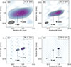 |
Fig. 1. KVN multifrequency images of 3C 138 at 21.8, 43.3, 86.4, and 129.4 GHz obtained on 2024 December 12. Contours are drawn at ( − 1, 1, 2, 4, …) × 5σ, where σ is the image rms noise. The synthesized beam is shown in the lower-left corner of each panel. Yellow circles denote circular two-dimensional Gaussian model components. Their diameters represent the fitted full widths at half maximum, and their centers mark the component positions. |
KVN image parameters.
Via Gaussian model fitting, we identified two components separated by about 5 mas, with the fainter eastern component lying to the southeast of the brighter western one at a position angle (PA) of about 105° (Table C.2). The eastern component is clearly resolved, with fitted sizes larger than the minimum resolvable size, whereas the western component is more compact and is constrained as an upper limit in some bands (Lobanov 2005). The component flux densities and most fitted component sizes remain consistent between the two epochs within the measurement uncertainties. The larger 86 GHz size of the western component in the second epoch is likely influenced mainly by poorer data quality and calibration effects. The 23.5 GHz VLBA results show two components with a similar separation and PA to those measured with the KVN (Fig. B.1). Unlike the eastern component, which remains approximately stable on year timescales, the western component brightened by a factor of about 2.6 from 2022 to 2025 (Table C.4). On kiloparsec scales, VLA images reveal a northeastward jet with a PA of approximately 40°–60° (Table C.6), indicating a clear PA offset between the compact two-component structure and the extended jet. As shown in Fig. B.2, the VLA core brightens substantially toward the high-frequency bands from 2022 to 2025, while the jet flux varies only weakly. This behavior implies that the observed increase in the integrated VLA flux is dominated by the core component.
3.2. Spectral analysis
The simultaneous four-band KVN observations enabled us to determine the spectra of the two components and identify the core. Figure 2 presents the spectra of the first epoch. The western component exhibits an apparently flatter spectrum than the eastern one, with an inverted slope between 22 and 43 GHz, which is characteristic of an SSA core. We therefore fitted the eastern component with a single power law (PL), Sν ∝ να, where α is the spectral index, and modeled the western component with a single-zone SSA model (Türler et al. 2000):
![Mathematical equation: $$ \begin{aligned} S_\nu = S_{\rm m} \left(\frac{\nu }{\nu _{\rm m}}\right)^{\alpha _{\rm t}} \frac{1-\exp \left[-\,\tau _{\rm m}\left(\nu /\nu _{\rm m}\right)^{\alpha _{\rm t}-\alpha _0}\right]}{1-\exp \left(-\tau _m\right)}, \end{aligned} $$](/articles/aa/full_html/2026/06/aa59759-26/aa59759-26-eq1.gif) (1)
(1)
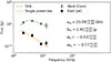 |
Fig. 2. Spectra of the two KVN-resolved components in 3C 138 on 2024 December 12. Open circles denote the western component (core), fitted with an SSA model (dash-dotted green curve), with turnover frequency νm, peak flux density Sm, and optically thin spectral index α0. Filled squares denote the eastern component (jet knot), fitted with a PL model (dashed orange line) with spectral index αPL. Error bars indicate 1σ uncertainties. |
where αt and α0 are the thick and thin spectral indices, and νm and Sm are the SSA turnover frequency and peak flux density. The spectral fitting results for the two components are shown in Fig. 2.
To probe the time variability of the broadband spectrum, we interpolated the ALMA flux densities using Gaussian-process (GP) regression, paired them with the four VLA epochs, and fitted the combined VLA+ALMA spectra with both a PL model and a PL+SSA model for each epoch. We then selected the preferred model by comparing the reduced χ2 and the Bayesian information criterion. As the two arrays are not simultaneous, and have unmatched angular resolutions, these fits should be interpreted with caution. The best-fit parameters are presented in Table C.1, and the fitting results are plotted in Fig. B.3.
4. Discussion
4.1. SSA core spectrum and temporal evolution
The KVN western component shows a flat–inverted spectrum between 22 and 43 GHz and is well described by an SSA model, supporting its identification as the SSA core. The eastern feature follows a single steep PL, consistent with an optically thin inner jet component (Fig. 2).
For the VLA data, as shown in Fig. B.3, a spectral inflection is detected only in 2024 and 2025, whereas the 2022–2023 spectra are adequately described by a single steep PL. This indicates a transition from a PL-only state to a PL+SSA state. Within the PL+SSA state, the optically thin slope (α0) of the SSA component further steepens, suggesting the high-energy electron population is evolving. If driven by a propagating shock, one would expect enhanced millimeter polarization, systematic electric vector position angle (EVPA) evolution, and higher-frequency light-curve peaks to precede those at lower frequencies.
Because the VLA flux increase is core-dominated (Sect. 3.1) and the VLA core blends the two KVN components, the integrated VLA+ALMA behavior can be used as a qualitative proxy for the SSA evolution of the KVN core. The turnover frequency inferred from VLA+ALMA is systematically higher than that from the KVN core, which may reflect residual mixing with optically thin emission and/or intrinsic inhomogeneity within the KVN core region, such that a one-zone SSA model yields an effective turnover frequency.
4.2. Magnetic field strength
We estimated the SSA magnetic field strength and the equipartition magnetic field strength of the KVN core for the first epoch (2024 December 12) using the SSA spectral parameters listed in Fig. 2, together with the SSA region size (dm) scaled from the bright-state VLBA core size and the Doppler factor (δ) estimated from VLBA core variability (Appendix A).
We adopted dm = 0.07 ± 0.01 mas and  , noting that δvar is an approximate constraint and likely a lower limit given the sparse temporal sampling and possible unresolved substructure. Using these parameters, we derived
  mG and
  mG, which yields
  . This indicates that the SSA core is particle-dominated.
The dominant uncertainty arises from dm (scaled from the VLBA core size). We propagated uncertainties via Monte Carlo sampling, and we further tested the sensitivity of the result to the assumed geometric and opacity scalings by varying jet-opening index and the core-shift index within plausible ranges. In all cases, we obtain BSSA/Beq ≪ 1 (Fig. A.2), so the particle-dominated conclusion is robust.
4.3. Core brightening and high-energy emission
Multifrequency, multi-scale data show that the flux rise since 2022 is core-dominated (Fig. B.2), meaning a kiloparsec-scale jet–interstellar medium interaction is likely not the primary driver of the integrated flux increase. VLBA images show a steady brightening of the western core, while the eastern knot and the kiloparsec-scale VLA jet remain nearly constant, pointing to processes within the VLBI core.
The KVN SSA core magnetic field strength is far below the equipartition value, implying a particle-dominated region and an increase in synchrotron emitting electrons, possibly associated with shock-driven particle acceleration. ALMA polarization monitoring further shows a gradual increase in polarized flux after 2022 (Kameno et al. 2025), consistent with a more ordered magnetic field.
If a shock is responsible, a new component may be forming but still unresolved. Using the inverted minimum-resolvable-size relation, we find that the image rms required to resolve a separation of two KVN core sizes is 5.71, 19.1, 2.10, and 17.3 mJy at 22, 43, 86, and 129 GHz in the first epoch, and 0.8, 1.2, and 1.7 mJy in the second epoch at 22, 43, and 86 GHz, which is comparable to or higher than our achieved rms at each frequency at both epochs. Yet no new component is detected near the core, suggesting that any emerging feature remains blended with the core and has not reached a resolvable downstream separation.
Using the inferred δvar, we estimate that the corresponding apparent speed is at most of order 2c, corresponding to a proper motion of about 0.05 mas yr−1. Under a separability criterion of two VLBA core sizes (about 0.12 mas), a newly emerging component would therefore require at least a few years to become clearly separated from the core. If the viewing angle is instead as large as θ = 34°, as inferred by Shen et al. (2001), then the corresponding separation timescale would be even longer.
Either case implies only mild Doppler boosting. Nevertheless, with efficient acceleration, inverse-Compton processes can produce X-ray to gamma-ray radiation under modest Doppler boosting, as suggested by Fermi-LAT detections of young radio galaxies and compact symmetric objects (e.g., PKS 1718-649 and NGC 3894; Migliori et al. 2016; Principe et al. 2020, 2021). Continued high-frequency, high-resolution polarization VLBI observations will allow us to test this scenario by constraining the emergence timescale of a new component and by tracking polarization and EVPA evolution in the core.
5. Conclusion
Using two-epoch, four-band KVN imaging of the CSS source 3C 138, we identified the western of the two KVN-resolved components as the SSA core. The turnover frequency inferred from the integrated VLA+ALMA spectra is higher than that from the KVN core spectrum, which can be attributed to resolution blending of the compact core with additional emitting regions in the lower-resolution data. The multi-year radio brightening is core-dominated and the core magnetic field is below equipartition, implying a particle-dominated emitting region with only mild Doppler boosting. Shock-driven particle injection in the inner jet could account for the contemporaneous X-/gamma-ray emission without extreme beaming. Although no new knot is resolved, a slowly emerging feature may still be blended within the VLBI core. Continued high-frequency, high-resolution VLBI monitoring will be needed to test this scenario.
Acknowledgments
We are grateful to the staff of the KVN who helped to operate the array and to correlate the data. The KVN and a high-performance computing cluster are facilities operated by the KASI (Korea Astronomy and Space Science Institute). The KVN observations and correlations are supported through the high-speed network connections among the KVN sites provided by the KREONET (Korea Research Environment Open NETwork), which is managed and operated by the KISTI (Korea Institute of Science and Technology Information). This work is supported by the National Research Foundation of Korea (NRF) grant funded by the Korea government (MSIT) (2020R1A2C2009003, RS-2025-00562700). The authors acknowledge use of the Very Long Baseline Array under the US Naval Observatory’s time allocation. This work supports USNO’s ongoing research into the celestial reference frame and geodesy. This work also made use of data from the Very Large Array operated by the National Radio Astronomy Observatory (NRAO). The NRAO and the Green Bank Observatory are facilities of the U.S. National Science Foundation operated under cooperative agreement by Associated Universities, Inc. This work makes use of ALMA data (ADS/JAO.ALMA#2011.0.00001.CAL). ALMA is a partnership of ESO, NSF (USA), and NINS (Japan), together with NRC (Canada), NSTC/ASIAA (Taiwan), and KASI (Republic of Korea), in cooperation with the Republic of Chile. The Joint ALMA Observatory is operated by ESO, AUI/NRAO, and NAOJ.
References
- Algaba, J.-C., Nakamura, M., Asada, K., & Lee, S.-S. 2017, ApJ, 834, 65 [Google Scholar]
- Atwood, W. B., Abdo, A. A., Ackermann, M., et al. 2009, ApJ, 697, 1071 [CrossRef] [Google Scholar]
- Bronzini, E., Cheung, C. C., & La Mura, G. 2024, ATel, 16845, 1 [Google Scholar]
- CASA Team (Bean, B., et al.) 2022, PASP, 134, 114501 [NASA ADS] [CrossRef] [Google Scholar]
- Cotton, W. D., Dallacasa, D., Fanti, C., et al. 2003, A&A, 406, 43 [NASA ADS] [CrossRef] [EDP Sciences] [Google Scholar]
- Fanti, C., Fanti, R., Parma, P., et al. 1989, A&A, 217, 44 [NASA ADS] [Google Scholar]
- Fomalont, E. B. 1999, ASP Conf. Ser., 180, 301 [NASA ADS] [Google Scholar]
- Fuhrmann, L., Krichbaum, T. P., Witzel, A., et al. 2008, A&A, 490, 1019 [NASA ADS] [CrossRef] [EDP Sciences] [Google Scholar]
- Giacchino, F., Monti-Guarnieri, P., & La Mura, G. 2025, ATel, 17142, 1 [Google Scholar]
- Greisen, E. W. 2003, Astrophys. Space Sci. Lib., 285, 109 [NASA ADS] [Google Scholar]
- Hewitt, A., & Burbidge, G. 1989, ApJS, 69, 1 [NASA ADS] [CrossRef] [Google Scholar]
- Hodgson, J. A., Lee, S.-S., Zhao, G.-Y., et al. 2016, JKAS, 49, 137 [Google Scholar]
- Hovatta, T., Valtaoja, E., Tornikoski, M., & Lähteenmäki, A. 2009, A&A, 494, 527 [CrossRef] [EDP Sciences] [Google Scholar]
- Kameno, S., Artur, E., Asaki, Y., et al. 2025, ATel, 17193, 1 [Google Scholar]
- Kang, S., Lee, S.-S., Hodgson, J., et al. 2021, A&A, 651, A74 [NASA ADS] [CrossRef] [EDP Sciences] [Google Scholar]
- Kataoka, J., & Stawarz, Ł. 2005, ApJ, 622, 797 [NASA ADS] [CrossRef] [Google Scholar]
- Kneissl, R., Plarre, K., Radiszcz, M., et al. 2023, ALMA at 10 years: Past, Present, and Future, 55 [Google Scholar]
- Lee, S.-S., Lobanov, A. P., Krichbaum, T. P., et al. 2008, AJ, 136, 159 [Google Scholar]
- Lee, S.-S., Wajima, K., Algaba, J.-C., et al. 2016, ApJS, 227, 8 [Google Scholar]
- Lobanov, A. P. 1998, A&A, 330, 79 [NASA ADS] [Google Scholar]
- Lobanov, A. P. 2005, ArXiv e-prints [arXiv:astro-ph/0503225] [Google Scholar]
- Marscher, A. P. 1983, ApJ, 264, 296 [Google Scholar]
- McMullin, J. P., Waters, B., Schiebel, D., Young, W., & Golap, K. 2007, ASP Conf. Ser., 376, 127 [Google Scholar]
- Migliori, G., Siemiginowska, A., Sobolewska, M., et al. 2016, ApJ, 821, 31 [NASA ADS] [CrossRef] [Google Scholar]
- O’Dea, C. P. 1998, PASP, 110, 493 [Google Scholar]
- O’Dea, C. P., & Saikia, D. J. 2021, A&ARv, 29, 3 [Google Scholar]
- Pearson, T. J. 1995, ASP Conf. Ser., 82, 267 [NASA ADS] [Google Scholar]
- Perley, R. A., & Butler, B. J. 2017, ApJS, 230, 7 [NASA ADS] [CrossRef] [Google Scholar]
- Principe, G., Migliori, G., Johnson, T. J., et al. 2020, A&A, 635, A185 [NASA ADS] [CrossRef] [EDP Sciences] [Google Scholar]
- Principe, G., Di Venere, L., Orienti, M., et al. 2021, MNRAS, 507, 4564 [NASA ADS] [CrossRef] [Google Scholar]
- Shen, Z.-Q., Jiang, D. R., Kameno, S., & Chen, Y.-J. 2001, A&A, 370, 65 [NASA ADS] [CrossRef] [EDP Sciences] [Google Scholar]
- Shepherd, M. C. 1997, ASP Conf. Ser., 125, 77 [Google Scholar]
- Sotnikova, Y. V., Mufakharov, T. V., Erkenov, A. K., et al. 2025, ATel, 17104, 1 [Google Scholar]
- Torniainen, I., Tornikoski, M., Teräsranta, H., Aller, M. F., & Aller, H. D. 2005, A&A, 435, 839 [NASA ADS] [CrossRef] [EDP Sciences] [Google Scholar]
- Türler, M., Courvoisier, T. J.-L., & Paltani, S. 2000, A&A, 361, 850 [Google Scholar]
- Wagner, S. 2025, ATel, 17180, 1 [Google Scholar]
- Wright, E. L. 2006, PASP, 118, 1711 [NASA ADS] [CrossRef] [Google Scholar]
Appendix A: Magnetic field strength estimates
This appendix provides the details of the magnetic-field calculations presented in Sect. 4.2.
A.1. Size scaling for the SSA region
The 23.5 GHz VLBA core appears larger in the fainter epoch (2022) but becomes much smaller in the brighter epochs (2024–2025; Table C.4). This behavior is consistent with the faint-state core being effectively broadened by blending of multiple sub-components within the finite VLBA resolution, whereas the bright-state emission is dominated by a more compact region. We therefore adopt the 2025 June VLBA core size (dVLBA = 0.06 ± 0.01 mas), measured in a bright-state epoch close in time to the KVN observations and with a well-constrained model fit (e.g., a fitted size exceeding the minimum resolvable size), as the reference size to scale the SSA region angular size dm, following
![Mathematical equation: $$ \begin{aligned} d_{\rm m} = 1.6\,d_{\rm VLBA} \left(\frac{\nu _{\rm m}}{\nu _{\rm VLBA}}\right)^{-\epsilon /k_{\rm r}}\ [\mathrm {mas}]\,, \end{aligned} $$](/articles/aa/full_html/2026/06/aa59759-26/aa59759-26-eq6.gif) (A.1)
(A.1)
where the factor 1.6 converts the full width at half maximum of a circular Gaussian component to the equivalent angular diameter of a uniform disk (Pearson 1995), ϵ describes the jet opening (ϵ ≃ 1 for a conical jet and ϵ < 1 for a collimating flow), and kr is the index that characterizes the frequency dependence of the core position, rcore ∝ ν−1/kr (Lobanov 1998). We adopt kr = 1 as a commonly used empirical value in core-shift scaling (Lobanov 1998), and the median ϵ value of 0.97 from Algaba et al. (2017).
A.2. Variability Doppler factor
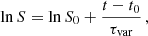
We estimate the variability Doppler factor from the temporal evolution of the VLBA core flux density S(t) at 23.5 GHz. Following Eq. (A.2), we fit the VLBA core light curve in log space with a least-squares method,
 (A.2)
(A.2)
where the fitted slope equals 1/τvar (Fig. A.1), and τvar is the variability timescale in days.
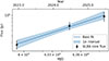 |
Fig. A.1. VLBA core light curve at 23.5 GHz from 2022 to 2025. The solid line is a least-squares fit, and the shaded region marks the 1σ confidence band. Black points show the measured core flux densities with 1σ errors. |
We then estimate the observed variability brightness temperature  , assuming that the variability is dominated by a circular Gaussian emitting region (Kang et al. 2021):
 (A.3)
(A.3)
where z is the redshift, DL is the luminosity distance in Mpc, ν is the observing frequency in GHz, and ΔS (Jy) is the flux density difference between the peak and the value at peak/e.
Assuming an equipartition brightness temperature (TB, eq) as the maximum intrinsic brightness temperature, the variability Doppler factor can be estimated (e.g., Fuhrmann et al. 2008; Hovatta et al. 2009; Kang et al. 2021) as
 (A.4)
(A.4)
Here we adopt TB, eq = 5 × 10¹⁰ K (Hovatta et al. 2009).
Given the sparse sampling of the VLBA core flux density (three epochs) and the possibility of unresolved substructure within the VLBA core, the derived τvar should be regarded as an upper limit. Consequently,  and δvar are likely underestimated, and δvar should be treated as an approximate constraint and potentially a lower limit.
A.3. Magnetic field strength formulae
Given Sm, νm, and α0 from the SSA fit (Fig. 2), together with dm and δvar, we compute the SSA magnetic field strength from Marscher (1983):
![Mathematical equation: $$ \begin{aligned} B_{\rm SSA}=10^{-2}\,b(\alpha _0)\, \left(\frac{S_{\rm m}}{\mathrm{Jy}}\right)^{-2} \left(\frac{d_{\rm m}}{\mathrm{mas}}\right)^{4} \left(\frac{\nu _{\rm m}}{\mathrm{GHz}}\right)^{5} \left(\frac{\delta }{1+z}\right)^{-1}\ [\mathrm{mG}]\,, \end{aligned} $$](/articles/aa/full_html/2026/06/aa59759-26/aa59759-26-eq12.gif) (A.5)
(A.5)
where b(α0) is a factor that depends on the optically thin spectral index, and δ is the Doppler factor.
The equipartition magnetic field strength is estimated following Kataoka & Stawarz (2005):
![Mathematical equation: $$ \begin{aligned} B_{\rm eq}&= 1.23\times 10^{-4}\, \eta ^{2/7}(1+z)^{11/7} \left(\frac{D_{\rm L}}{100\ \mathrm{Mpc}}\right)^{-2/7} \nonumber \\&\quad \times \left(\frac{\nu _{\rm m}}{5\ \mathrm{GHz}}\right)^{1/7} \left(\frac{S_{\rm m}}{100\ \mathrm{mJy}}\right)^{2/7} \left(\frac{10^3 d_{\rm m}}{0.3\ \mathrm{arcsec}}\right)^{-6/7} \delta ^{-5/7}\ \mathrm{[G]}\,, \end{aligned} $$](/articles/aa/full_html/2026/06/aa59759-26/aa59759-26-eq13.gif) (A.6)
(A.6)
assuming η = 1 (the ratio of proton + electron to electron energy densities).
The inferred BSSA is proportional to δ−1, Beq to δ−5/7, and thus BSSA/Beq to δ−2/7. Since δvar is likely underestimated, the derived BSSA, Beq, and BSSA/Beq should be interpreted as upper limits, subject to a corresponding systematic uncertainty.
A.4. Uncertainty propagation and sensitivity tests
The dominant uncertainty in the magnetic field estimates arises from the SSA region angular size dm, which is scaled from the VLBA core size dVLBA (Eq. A.1). The VLBA core size dVLBA at 23.5 GHz is obtained from circular Gaussian model fitting, and the statistical uncertainties of the fitted parameters are estimated from the post-fit image rms and the component signal-to-noise ratio using the first order approximation of Fomalont (1999).
To account for the strong non-linearity of Eqs. (A.1)–(A.6), we propagated uncertainties via Monte Carlo sampling by drawing Sm, νm and α0 from the SSA-fit posterior and dVLBA from its inferred distribution. In addition, we explored the impact of the geometric and opacity scalings in Eq. (A.1) by varying the jet-opening index (ϵ) and the core-shift index (kr) within plausible ranges (Fig. A.2).
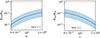 |
Fig. A.2. Left: Dependence of BSSA/Beq on the core-shift index (kr). Right: Dependence of BSSA/Beq on the jet opening (ϵ). |
Appendix B: Additional images and plots
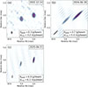 |
Fig. B.1. VLBA images of 3C 138 at 23.5 GHz obtained on 2022 December 14 (a), 2024 June 18 (b), and 2025 June 21 (c). Contours are drawn at ( − 1, 1, 2, 4, …) × 5σ, where σ is the image rms noise. The synthesized beam is shown in the lower-left corner of each panel. Yellow circles denote circular two-dimensional Gaussian model components. Their diameters represent the full widths at half maximum, and their centers mark the component positions. |
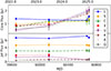 |
Fig. B.2. VLA core (top) and jet (bottom) flux densities at 1.5 (L), 3.0 (S), 5.5 (C), 9.0 (X), 14.0 (U), 22.2 (K), 32.0 (A), and 40.1 (Q) GHz as a function of time. |
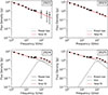 |
Fig. B.3. Quasi-simultaneous VLA+ALMA broadband spectra and PL/PL+SSA fits. Solid markers represent VLA observed data, open markers represent GP-interpolated ALMA data (see Sect. 3.2). |
Appendix C: Additional tables
PL+SSA fits to the VLA+ALMA spectra.
Model-fit parameters of the KVN components.
VLBA image parameters.
Model-fit parameters of the VLBA components.
VLA image parameters.
Model-fit parameters of the VLA components.
All Tables
All Figures
|
Fig. 1. KVN multifrequency images of 3C 138 at 21.8, 43.3, 86.4, and 129.4 GHz obtained on 2024 December 12. Contours are drawn at ( − 1, 1, 2, 4, …) × 5σ, where σ is the image rms noise. The synthesized beam is shown in the lower-left corner of each panel. Yellow circles denote circular two-dimensional Gaussian model components. Their diameters represent the fitted full widths at half maximum, and their centers mark the component positions. |
| In the text | |
|
Fig. 2. Spectra of the two KVN-resolved components in 3C 138 on 2024 December 12. Open circles denote the western component (core), fitted with an SSA model (dash-dotted green curve), with turnover frequency νm, peak flux density Sm, and optically thin spectral index α0. Filled squares denote the eastern component (jet knot), fitted with a PL model (dashed orange line) with spectral index αPL. Error bars indicate 1σ uncertainties. |
| In the text | |
|
Fig. A.1. VLBA core light curve at 23.5 GHz from 2022 to 2025. The solid line is a least-squares fit, and the shaded region marks the 1σ confidence band. Black points show the measured core flux densities with 1σ errors. |
| In the text | |
|
Fig. A.2. Left: Dependence of BSSA/Beq on the core-shift index (kr). Right: Dependence of BSSA/Beq on the jet opening (ϵ). |
| In the text | |
|
Fig. B.1. VLBA images of 3C 138 at 23.5 GHz obtained on 2022 December 14 (a), 2024 June 18 (b), and 2025 June 21 (c). Contours are drawn at ( − 1, 1, 2, 4, …) × 5σ, where σ is the image rms noise. The synthesized beam is shown in the lower-left corner of each panel. Yellow circles denote circular two-dimensional Gaussian model components. Their diameters represent the full widths at half maximum, and their centers mark the component positions. |
| In the text | |
|
Fig. B.2. VLA core (top) and jet (bottom) flux densities at 1.5 (L), 3.0 (S), 5.5 (C), 9.0 (X), 14.0 (U), 22.2 (K), 32.0 (A), and 40.1 (Q) GHz as a function of time. |
| In the text | |
|
Fig. B.3. Quasi-simultaneous VLA+ALMA broadband spectra and PL/PL+SSA fits. Solid markers represent VLA observed data, open markers represent GP-interpolated ALMA data (see Sect. 3.2). |
| In the text | |
Current usage metrics show cumulative count of Article Views (full-text article views including HTML views, PDF and ePub downloads, according to the available data) and Abstracts Views on Vision4Press platform.
Data correspond to usage on the plateform after 2015. The current usage metrics is available 48-96 hours after online publication and is updated daily on week days.
Initial download of the metrics may take a while.