


| Issue |
A&A
Volume 709, May 2026
|
|
|---|---|---|
| Article Number | A247 | |
| Number of page(s) | 14 | |
| Section | Astrophysical processes | |
| DOI | https://doi.org/10.1051/0004-6361/202659285 | |
| Published online | 25 May 2026 | |
Cyclotron lines in subcritical X-ray pulsars: Monte Carlo simulations reveal the origin of the observed variability
1
University of Crete, Department of Physics & Institute of Theoretical & Computational Physics, 70013 Heraklion, Greece
2
Institute of Astrophysics, Foundation for Research and Technology-Hellas, 71110 Heraklion, Crete, Greece
3
Department of Astrophysical Sciences, Peyton Hall, Princeton University, Princeton, NJ 08544, USA
4
Max-Planck-Institut für extraterrestrische Physik, Postfach 1312, 85741 Garching, Germany
5
University Observatory, Faculty of Physics, Ludwig-Maximilians Universität, Scheinerstr. 1, 81679 Munich, Germany
★ Corresponding authors: This email address is being protected from spambots. You need JavaScript enabled to view it.
, This email address is being protected from spambots. You need JavaScript enabled to view it.
, This email address is being protected from spambots. You need JavaScript enabled to view it.
Received:
2
February
2026
Accepted:
30
March
2026
Abstract
Context. Observed cyclotron resonant scattering features (CRSFs) in X-ray pulsars (XRPs) exhibit strong variability. In the subcritical luminosity regime, the centroid energy (ECRSF) and line width (σCRSF) often show positive correlations with the X-ray luminosity.
Aims. We investigate the physical origin of the observed variability quantitatively, focusing on the effects of resonant scattering and Doppler shift induced by the plasma flow in the accretion funnel.
Methods. We developed a relativistic Monte Carlo code to perform detailed radiative transfer calculations in the accretion funnel above the hotspot and derived angle-dependent spectra. We adopted analytical plasma density and velocity profiles to account for the effects of radiation pressure on the flow, and we employed approximate resonant scattering cross sections. We varied the accretion luminosity to explore the resulting variability of the CRSF properties.
Results. The emergent spectra exhibit a prominent, asymmetric CRSF accompanied by a broad blue wing. The CRSF is systematically redshifted relative to the classical cyclotron energy, with the magnitude of the redshift decreasing at higher luminosities and for larger viewing angles θ. Both ECRSF and σCRSF correlate positively with luminosity for all viewing angles. Their absolute values, however, depend strongly on the viewing angle, indicating substantial variability over the pulse cycle and sensitivity to the system geometry. At a fixed luminosity, ECRSF (σCRSF) decreases (increases) with increasing cos θ. Consequently, our model predicts that phase-resolved observations will reveal an anticorrelation between the CRSF centroid energy and width. When applied to the XRP GX 304−1, the model reproduces the observed CRSF variability over nearly an order of magnitude in luminosity for geometries in which the accretion funnel is predominantly viewed edge-on.
Conclusions. Resonant scattering of radiation propagating through the accreting plasma in the magnetic funnel provides a natural explanation for the observed CRSF variability in subcritical XRPs.
Key words: accretion, accretion disks / line: formation / magnetic fields / radiative transfer / stars: neutron / X-rays: binaries
© The Authors 2026
 Open Access article, published by EDP Sciences, under the terms of the Creative Commons Attribution License (https://creativecommons.org/licenses/by/4.0), which permits unrestricted use, distribution, and reproduction in any medium, provided the original work is properly cited.
This article is published in open access under the Subscribe to Open model. This email address is being protected from spambots. You need JavaScript enabled to view it. to support open access publication.
1. Introduction
Accretion-powered X-ray pulsars (XRPs) are highly magnetized neutron stars (NSs) in binary systems accreting from a companion, typically an OB supergiant or a Be star (for a recent review see Weng & Ji 2024). Due to the star’s strong magnetic field (usually a few 1012 G), accretion proceeds along the magnetosphere, and the plasma is channeled onto the magnetic poles (Ghosh & Lamb 1979). This process heats the magnetic polar regions, creates hotspots, and, under certain conditions, produces accretion columns, where the gravitational energy of the relativistic inflowing plasma is released primarily via hard X-ray emission (Basko & Sunyaev 1975, 1976; Arons et al. 1987).
A substantial fraction of these sources shows absorption-line-like features in the 10–100 keV energy range of their spectra, the so-called cyclotron lines or cyclotron resonant scattering features (CRSFs; for a review, see Staubert et al. 2019). These features originate from a quantum-mechanical process called magnetic scattering. The perpendicular momentum of charged particles in a strong magnetic field is quantized, resulting in discrete energy states, known as Landau levels (Landau 1930). Resonant scattering of photons with inflowing electrons in the vicinity of the NS surface imprints the fundamental CRSF in the continuum (Trümper et al. 1977; Truemper et al. 1978), with several XRPs also featuring harmonics (Truemper et al. 1978; Santangelo et al. 1999; Fürst et al. 2018; Yang et al. 2023). The energy difference between two successive Landau levels (hereafter referred to as the cyclotron energy) in the nonrelativistic case is
 (1)
(1)
where B is the magnetic field strength in the line forming region, ℏ is the reduced Planck constant, me is the electron’s rest mass, c is the speed of light, and e is the elementary charge. As Ec is linearly proportional to the magnetic field, the detection of CRSFs provides a direct and robust means of measuring the magnetic field strength in XRPs and, more broadly, serves as a diagnostic of the physical conditions near the neutron star surface Gnedin & Sunyaev (1974).
Detailed observations of CRSFs in XRPs have revealed significant variability both with pulse phase and X-ray luminosity, L (for reviews, see Staubert et al. 2019; Mushtukov & Tsygankov 2022). Pulse-phase modulations indicate anisotropic emergent spectra (e.g., Maniadakis et al. 2025), whereas variations with L (accretion rate) hint at changes in the emission region (e.g., Shui et al. 2024). Evidence of long-term CRSF variability has also been observed in Her X-1 (Staubert et al. 2017; Xiao et al. 2019), but the underlying physical mechanism remains unclear.
Of particular interest is the dependence of the observed CRSF centroid energy, ECRSF, on the X-ray luminosity, L. Such behavior has been reported in several XRPs, including V0332+53 (Tsygankov et al. 2006, 2010), GX 304−1 (Klochkov et al. 2012; Malacaria et al. 2015; Rothschild et al. 2017), and GRO J1008−57 (Chen et al. 2021). High-luminosity sources (L ≳ 1037 erg s−1) typically present a negative correlation between ECRSF and L, whereas in low-luminosity sources (L ≲ 1037 erg s−1) the trend reverses, with a positive correlation emerging. A complete transition from positive to negative correlation has recently been identified in pulse-to-pulse analyses of 1A 0535+262 by Shui et al. (2024), further reinforcing this distinction among sources. The leading physical explanation is the emergence of an accretion column once the luminosity exceeds a critical value, L* ∼ 1037 erg s−1 (Basko & Sunyaev 1976; Mushtukov et al. 2015a), signaling a transition in the accretion regime (Becker et al. 2012); from a surface-dominated hotspot regime (L ≲ L*) to an accretion-column regime (L ≳ L*).
For supercritical (accretion-column-dominated) sources, it has been shown analytically (Basko & Sunyaev 1976; Becker & Wolff 2007) and through first-principles radiation-magnetohydrodynamic (RMHD) simulations (Klein et al. 1996; Zhang et al. 2022, 2023, 2025a) that the braking of the infalling plasma is caused by an extended radiation-mediated shock (RS) forming in the magnetically confined, optically thick, accretion column. Both analytical studies (Basko & Sunyaev 1976) and Monte Carlo (MC) approaches (Loudas et al. 2024b) support the RS as the likely formation site of CRSFs in high luminosity XRPs. This scenario successfully predicts the observed anti-correlation between ECRSF and L: As the accretion rate increases, the accretion column grows in height, while the magnetic field strength drops with altitude. Thus, the cyclotron energy in the line-forming region shifts to lower values at higher luminosities (Burnard et al. 1991; Loudas et al. 2024a). An alternative scenario, proposed by Poutanen et al. (2013), attributes CRSF formation to surface reflection of hard X-rays emitted from the accretion column, but detailed radiative-transfer simulations challenge the viability of this interpretation (Kylafis et al. 2021).
At low luminosities (hot-spot-dominated emission), the outgoing radiation is dynamically unimportant, the accreting plasma reaches the NS surface in free fall, and the formation of CRSFs is believed to occur within the NS atmosphere. Even though no settled theory exists explaining the deceleration of the falling material, two leading mechanisms are found in the literature: 1) braking of plasma in the atmosphere by Coulomb collisions (Zel’dovich & Shakura 1969; Miller et al. 1987; Sokolova-Lapa et al. 2021) and 2) emergence of a collisionless shock (CS) where the infalling plasma is thermalized upon passing through the shock (Bisnovatyi-Kogan & Fridman 1970; Langer & Rappaport 1982; Bykov & Krasil’Shchikov 2004). The former model considers spectral formation in the NS atmosphere and can explain the observed double-hump in the hard X-ray spectra of low-luminosity XRPs (Mushtukov et al. 2021; Sokolova-Lapa et al. 2021), but it predicts zero variability of the cyclotron line centroid with luminosity and thus cannot reproduce the observed trends of cyclotron lines.
Conversely, the CS scenario has been successful in explaining the positive correlation between ECRSF and L in several sources (Staubert et al. 2007; Vybornov et al. 2017; Rothschild et al. 2017; Roy & Sharma 2025). In that case, spectral formation takes place between the NS surface and the shock discontinuity. Since the magnetic field strength (and effectively ECRSF) increases as the altitude decreases, and the CS height decreases with accretion rate (luminosity L) (Bykov & Krasil’Shchikov 2004), a positive correlation between ECRSF and L arises (see also Becker et al. 2012). However, first-principles kinetic simulations are required to address whether the formation of such a shock is feasible under conditions encountered above the NS atmosphere and determine its properties. Once the shock dynamics is understood, subsequent radiative transfer calculations need to be conducted, followed by comparison with observed spectra and pulse profiles.
Mushtukov et al. (2015b) pointed out that for subcritical luminosities (L ≲ L*) even though the propagation of the hotspot’s radiation through the mildly relativistic infalling plasma cannot halt accretion, it can significantly modify the velocity and density profiles above the NS surface. This effect was verified by robust RMHD simulations by Markozov et al. (2023). In this scenario, the formation of the CRSF takes place above the hotspot. Upward-propagating X-rays undergo resonant scattering with the infalling electrons, producing a redshifted CRSF relative to the local cyclotron energy due to the Doppler effect between the laboratory frame (hotspot) and the moving electron’s bulk frame. This model predicts a positive correlation between ECRSF and L without postulating the presence of a CS. A qualitative explanation follows. Radiation pressure acts to decelerate the accretion flow, influencing the degree of redshift in the CRSF. As luminosity (and hence radiation pressure) increases, the accretion-flow velocity right above the hotspot decreases, reducing the Doppler shift and shifting the CRSF centroid to higher energies (closer to the local Ec). Although the model shows promise and has been successful in qualitatively explaining observations of the X-ray pulsar GX 304−1 (Mushtukov et al. 2015b), no quantitative calculations of cyclotron line formation and variability have yet been carried out within this framework.
In this paper, we investigate the aforementioned model by conducting robust MC radiative transfer simulations to obtain the angle-resolved spectrum for a typical X-ray pulsar, focusing on the properties of the emergent CRSF, and studying its dependence on accretion rate. We aim to quantitatively test the following predictions made by Mushtukov et al. (2015b):
-
(i)
ECRSF is positively correlated with the luminosity L.
-
(ii)
The line width, σCRSF, is positively correlated with L.
-
(iii)
Both ECRSF and σCRSF vary significantly over the pulse phase.
The structure of this paper is organized as follows. In Sect. 2, we introduce the physical model, detailing the velocity and density profiles, along with the structure of the accretion channel. In Sect. 3, we provide a detailed description of our MC code. In Sect. 4, we present the simulated spectra for a typical X-ray pulsar and analyze their primary features. In Sect. 5, we compare our MC results with observational data from GX 304−1 and discuss the degeneracies inherent in the methodology. In Sect. 6, we comment on the results and draw our conclusions.
2. The model
In this section, we outline the underlying features of the model developed by Mushtukov et al. (2015b), which applies to sources in the subcritical luminosity regime (L ≲ L*).
2.1. Structure of the accretion funnel
We considered magnetospheric accretion onto the magnetic pole of a highly magnetized NS. The strong magnetic field confines the accretion flow into a funnel, and the plasma moves along the field lines only. The impact of infalling plasma heats the NS atmosphere at the base of the funnel, forming a hotspot that produces an outgoing photon beam. For simplicity, we adopted a cylindrical geometry for the filled accretion column, although more realistic accretion flow models favor bow-shaped or annular hotspots (Basko & Sunyaev 1976; Romanova et al. 2004; Zhu 2025). We injected seed photons isotropically upward from the base of the cylinder with a blackbody spectrum. We further assumed a uniform magnetic field B aligned with the magnetic axis, i.e.,  . This approximation is justified because the vertical extent of the line-forming region and the size of the funnel are, by construction, much smaller than the NS radius.
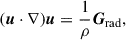
The interaction between upward-moving photons and the infalling electrons through Compton scattering exerts a drag (radiation-pressure) force on the falling plasma, altering its velocity and density profiles in a nontrivial manner. In the subcritical luminosity regime considered here, the plasma reaches the surface with a nonzero terminal velocity before being completely thermalized via Coulomb collisions in the atmosphere (Zel’dovich & Shakura 1969). Conservation of momentum in the nonrelativistic regime for a stationary flow dictates
 (2)
(2)
where ρ and u are the plasma density and bulk velocity, respectively, while Grad is the radiation-pressure force, proportional to the radiation flux times the opacity. In this equation, we neglected the gas pressure and gravity terms, as the radiation-pressure force is the dominant one in the vicinity of the NS surface. Mushtukov et al. (2015b) solved Eq. (2) and derived the following analytical expression for the velocity profile β(h)≡|u(h)|/c in the center of the column, considering isotropic emission from the hotspot, accounting for the dependence of the outgoing radiation flux on the height h above the NS surface, and considering motion along the field lines only,
![Mathematical equation: $$ \begin{aligned} \beta (h) = \left[\beta _{\rm ff}^2 - \left(\beta _{\rm ff}^2 - \beta _0^2\right) \left( 1 - \frac{2}{\pi }\tan ^{-1}\left(\frac{h}{d}\right)\right)\right]^{1/2}. \end{aligned} $$](/articles/aa/full_html/2026/05/aa59285-26/aa59285-26-eq4.gif) (3)
(3)
Here, d is the radius of the hotspot, estimated by the following power-law scaling (Mushtukov et al. 2015b)
 (4)
(4)
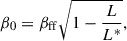
where Λ = 0.5 is a geometrical parameter related to the coupling of the magnetosphere to the disk (Ghosh & Lamb 1978), L37 ≡ L/1037 erg s−1, B12 ≡ B/1012 G, m = M/M⊙, and R6 ≡ R/106 cm. In Eq. (3), βff denotes the free-fall speed, divided by c, of the accreting plasma at the neutron-star surface, while β0 represents the terminal velocity at the stellar surface (h = 0). The latter is related to the accretion luminosity through energy conservation, assuming that the kinetic energy of the accreting plasma is instantaneously converted into radiation via thermalization at the hotspot and Compton scattering above it. This yields a scaling relation of the form
 (5)
(5)
with the critical luminosity L* defined as the limiting luminosity at which the infalling material is fully decelerated (β0 = 0) by radiation pressure at the stellar surface; above this threshold, an RS is expected to rise above the hotspot (Basko & Sunyaev 1976).
To ensure that the model is self-consistent, the velocity profile described by Eq. (3) necessitates a nonuniform density profile that obeys the conservation of mass
 (6)
(6)
Given the cylindrical geometry and a constant accretion rate (Ṁ = const), the electron number density profile reads (Mushtukov et al. 2015b)
 (7)
(7)
Finally, following Mushtukov & Tsygankov (2022) (see Sect. 4.3 therein), we estimate the effective temperature of the hotspot using the Stefan-Boltzmann law
 (8)
(8)
where σSB is the Stefan-Boltzmann constant and SD denotes the hotspot area, given by Mushtukov et al. (2015b)
 (9)
(9)
The factor of two in the denominator of Eq. (8) accounts for the existence of two antipodal hotspots.
The approximate power-law scaling adopted for the hotspot effective temperature captures the expected positive correlation with luminosity. However, the absolute normalization of the temperature remains uncertain at the level of a factor of ∼2, depending on the accretion geometry (e.g., the shape of the landing region, stochastic variability, and system inclination) and on the microphysics of the thermalization process in the NS atmosphere (e.g., CS versus Coulomb collisions). Deriving a robust prescription for temperature would require detailed RMHD simulations (such as those of Markozov et al. 2023) and is therefore beyond the scope of this work. Nevertheless, we emphasize that our conclusions regarding the CRSF properties and their dependence on luminosity and/or viewing angle are insensitive to the assumed injected photon spectrum, and hence to the specific choice of the hotspot (blackbody) temperature.
2.2. CRSF formation
As the accreting plasma descends toward the surface, upward-propagating photons undergo Compton scattering with the infalling electrons. For typical values of the electron density and hotspot size, the perpendicular Thomson optical depth of the accretion funnel lies in the optically thin regime,
 (10)
(10)
such that most photons escape without scattering. However, magnetic scattering includes resonant processes in which photons with energies near the cyclotron resonance experience a strongly enhanced cross section (up to ∼106σT, Canuto et al. 1971; Ventura 1979; Harding & Daugherty 1991; Sina 1996; Mushtukov et al. 2016; Loudas et al. 2021) and are effectively trapped within the medium. These resonant photons dominate the radiative deceleration of the infalling plasma (Mushtukov et al. 2015b): they undergo multiple resonant scatterings until they exchange sufficient energy with the electrons to shift out of resonance and escape the funnel. This process naturally produces an absorption-line-like feature accompanied by two broad, emission-like wings, reflecting photon redistribution in energy rather than true photon absorption, since the total number of photons is conserved in scattering.
In this study, we assumed that the magnetic field strength is well below the quantum electrodynamics (QED) critical value,
 (11)
(11)
such that the dimensionless field strength, b ≡ B/Bcr ≪ 1, and we also considered the infalling electron’s temperature Te to be substantially smaller than the local cyclotron energy, that is, kBTe ≪ Ec. In short, we restricted our analysis to systems that satisfy
 (12)
(12)
which is suitable for most XRPs in the hotspot regime (Becker & Wolff 2005). Under these conditions, the vast majority of electrons occupy the fundamental Landau level (n = 0), allowing us to safely limit our treatment to transitions between the ground state and the first excited Landau level (0 → 1 → 0) (Nobili et al. 2008; Loudas et al. 2021).
In the infalling electron’s rest frame, the relativistic cyclotron resonance energy is given by
 (13)
(13)
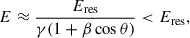
where θrf is the angle between the photon momentum and the magnetic field in the electron frame. For small values of b, one would expect the CRSF centroid energy to appear at Eres ≈ Ec. Due to the bulk motion of the infalling plasma, this resonance energy appears Doppler shifted when viewed from the laboratory frame; thus, it is not photons with energy ≈Eres (in the lab frame) that are in resonance, but those that the Doppler boost to the electron frame brings them in resonance, that is
 (14)
(14)
where θ ∈ (0, π/2) is the angle between the photon momentum and the magnetic field in the lab, and γ = (1 − β2)−1/2. Therefore, the CRSF will not form at Eres but will appear redshifted. As Eq. (14) indicates, the amount of redshift depends on the plasma’s velocity in the region where the interaction takes place, as well as on the photon’s direction of propagation.
Higher luminosities correspond to lower infall velocities (see Eq. (5)), leading to higher CRSF centroid energies. This results in a positive correlation between the luminosity and the CRSF centroid energy (Mushtukov et al. 2015b). In addition, for a given velocity, the Doppler redshift decreases with increasing viewing (propagation) angle θ, implying that the CRSF centroid energy increases with θ. However, this qualitative picture is based on the single-scattering approximation. Multiple scatterings could induce modulations in the shape and location of the emergent CRSF. Obtaining accurate predictions of the model requires full radiative-transfer calculations.
3. Monte Carlo code
The relativistic MC radiative transfer code employed in this work is based on the implementation developed by Loudas et al. (2024b), to which the reader is referred for a detailed description. Here, we summarize the main parts of the code and describe the improvements with respect to the version of Loudas et al. (2024b). Radiative transfer is treated using the forced first collision technique, which ensures efficient sampling of photon–electron interactions. Photon packets are injected in the accretion funnel and are followed by the MC code until they escape. A key advantage of the present implementation is its flexibility, as it supports arbitrary density and velocity profiles within the accretion channel, enabling direct tests of different physical scenarios. Moreover, it incorporates an adaptive step size algorithm that increases efficiency, while maintaining accuracy in regions of steep gradients. Figure 1 shows an illustration of the system’s geometry and the numerical propagation of a photon packet.
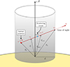 |
Fig. 1. Illustration of the MC code’s geometry, coordinates, and calculation of the line-of-sight optical depth. A photon packet located at r0 is moving in direction |

3.1. Accretion channel and plasma
We modeled the accretion channel as an axisymmetric cylindrical column of radius d and semi-infinite length, with its base located at the NS surface. We considered the magnetic field to be homogeneous along the z axis, that is,  , because the height of the line-forming region is much smaller than the NS radius. The electron density, ne(r), evaluated at r = (x, y, z = h) is given by Eq. (7), while the bulk velocity of the infalling plasma is taken to be
  , with β(r) computed by Eq. (3). Even though both density and velocity profiles are expected to differ across the column (Markozov et al. 2023), for the purposes of this work, we utilized the analytical 1D profiles derived by Mushtukov et al. (2015b). We treated infalling electrons as a cold plasma, an assumption justified by observations (Becker & Wolff 2005); thus we set Te = 0 in our simulations.
3.2. Seed photons
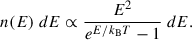
We emitted photon packets isotropically upward, with their initial positions sampled homogeneously from the base of the accretion channel. In our coordinate system, this base corresponds to the region ℛ = {(x, y, z = h)∈ℝ3 : x2 + y2 ≤ d2, h = 0}. We initialized each photon packet with a specified weight, w = N (typically 106), and assigned it an initial energy E drawn from a blackbody distribution at temperature T (given by Eq. 8),
 (15)
(15)
3.3. Optical depth calculation and photon propagation
We carried out the photon packet propagation as follows. We considered a photon packet with weight w, located at position r0 and propagating in direction  with energy E. Here, θ is the angle relative to the magnetic axis, while φ is the azimuthal one. The cumulative optical depth along the line of sight is defined as
 (16)
(16)
where the trajectory 𝒞 is a straight line extending from r0 to the cylindrical funnel’s boundary and ds is the infinitesimal scalar path length along 𝒞. The effective cross section σeff accounts for the bulk motion of the plasma and is defined as
 (17)
(17)
where σ is the magnetic scattering cross section expressed in terms of quantities evaluated at the electron rest frame (see Sect. 3.4) and β ≥ 0, by construction. The subscript “rf” denotes quantities measured in the electron rest frame. The Lorentz transformations relate the rest-frame quantities to the laboratory-frame ones as follows,
 (18)
(18)
and
 (19)
(19)
where γ = (1 − β2)−1/2.
To determine the location of the next scattering event, we computed numerically τn using an adaptive step-size algorithm to handle regions where the electron density ne(r) and/or β(r) vary rapidly. We discretized the integration path into a sequence of points r0, r1, …, rn along 𝒞, where rn is the point of the line-of-sight’s intersection with the column boundary. Given a point ri, we determined the subsequent point ri + 1 as follows. First, we calculated the local mean free path
![Mathematical equation: $$ \begin{aligned} \lambda _{i} \equiv \bar{\lambda } (\boldsymbol{r}_i, \hat{n}, E) = \left[ n_{\mathrm{e}}(\boldsymbol{r}_i) \, \sigma _{\mathrm{eff}}(E_{\rm rf},\boldsymbol{r}_i, \hat{n}_{\rm rf}) \right]^{-1}. \end{aligned} $$](/articles/aa/full_html/2026/05/aa59285-26/aa59285-26-eq25.gif) (20)
(20)
We then proposed a tentative step size equal to 1% of the local mean free path
 (21)
(21)
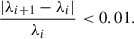
To ensure linearity over this step, we evaluated λi + 1 at the new location and enforced the relative error condition
 (22)
(22)
If condition (22) was violated, we rejected the step and redefined ri + 1 closer to ri by halving the step size (backtracking), that is by increasing the spatial resolution locally until the condition was satisfied,
 (23)
(23)
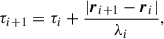
Once the step was accepted, the accumulated optical depth was updated as
 (24)
(24)
with the initial condition τ0 = 0. This process continues until the boundary is reached (or τ > 20 for efficiency), yielding the total optical depth τn. A fraction we−τn of the photon packet escapes the domain, and its energy and direction are recorded.
The remaining fraction underwent scattering with an electron in the column. The probability to scatter after covering a distance equivalent to optical depth τ is given by a truncated exponential distribution in τ, and thus we sampled a target optical depth τrnd using
![Mathematical equation: $$ \begin{aligned} \tau _{\rm rnd} = -\ln \left[ 1 - \xi \left(1 - e^{-\tau _n}\right) \right], \end{aligned} $$](/articles/aa/full_html/2026/05/aa59285-26/aa59285-26-eq30.gif) (25)
(25)
where ξ ∈ [0, 1) is a uniform random number; ξ = 0 implies scattering without moving forward at all, while ξ → 1 indicates that the photon packet will scatter right before it reaches the boundary. We then located the index i such that τi ≤ τrnd < τi + 1. We found the precise location of the next scattering event, rnew, via linear interpolation along the segment,
 (26)
(26)
where |ri − r0|≤|rnew − r0|< |ri + 1 − r0|.
Once the exact location of the scattering event was specified, we updated the weight of the remaining photon packet as follows,
 (27)
(27)
This formula ensures conservation of the total number of photons. If wnew was larger than 1, we carried out the scattering event as described below; otherwise, we proceeded to the injection and propagation of a new photon packet (Sect. 3.2).
We treated the scattering process in three steps. First, we Lorentz-transformed the photon-packet energy and propagation direction from the laboratory frame to the electron rest frame using the local bulk velocity evaluated at the scattering location rnew (Eqs. (18) and (19)). Next, we sampled a new photon propagation direction  in the electron rest frame employing the differential scattering cross section (see Sect. 3.4); specifically, we drew θrf′ from the cross section and sampled φ′rf isotropically. We then computed the post-scattering photon energy
  via energy conservation (Eq. (8) in Loudas et al. 2021). Finally, we applied the inverse Lorentz transformation to return to the laboratory frame and updated the photon-packet properties,
 (28)
(28)
after which the photon was propagated to the next interaction.
3.4. Prescription of resonant Compton scattering
In this work, we focus on the formation of the CRSF, so we need to adopt resonant magnetic scattering cross sections. Fully relativistic QED cross sections have been extensively studied (Harding & Daugherty 1991; Sina 1996; Nobili et al. 2008; Gonthier et al. 2014; Mushtukov et al. 2016), but they turn out to be cumbersome and the primary bottleneck in radiative transfer codes (see, e.g., Araya & Harding 1999; Schwarm et al. 2017; Kumar et al. 2022). To tackle this issue, Loudas et al. (2021) offers approximate, but accurate, resonant magnetic scattering cross sections that are applicable when b ≪ 1 and E ≪ mec2. Given that the systems of our interest lie in this regime, we adopt the resonant Compton scattering prescription developed by Loudas et al. (2021).
In this study, we neglected polarization effects; therefore, we employed the polarization-averaged differential cross section. In the electron’s rest frame, and integrated over the azimuthal angle φrf′, it is expressed as
 (29)
(29)
where θrf and θ′rf denote the incident and scattered photon angles relative to the magnetic field. The azimuthal averaging implies that, in our MC implementation, the azimuthal scattering angle is sampled isotropically; this is justified in our regime, where the resonant contribution dominates the spectral formation and is effectively independent of φ′rf (see, e.g., Ventura 1979). Here, L(Erf, Eres) is the resonance (Lorentz) line profile,
 (30)
(30)
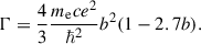
centered on the relativistic cyclotron energy, Eres (see Eq. (13)). For the relativistic cyclotron transition rate Γ, we used the first-order corrected expression (Loudas et al. 2021)
 (31)
(31)
The magnetic scattering cross section, σ, is the integral of the differential cross section (29) over θ′rf, namely
 (32)
(32)
We employed this expression in the calculation of the effective cross section (17).
3.5. Treatment of the boundary
Although most photons diffuse away from the base, where they are emitted, and escape, a small fraction of them return to the boundary (base). In this work, we do not model the physics of the NS atmosphere located below the base of the column (z < 0). So, when a photon packet reaches the base or when the line of sight intersects the base of the cylinder, a special treatment is required. If the wave packet crosses the base at z = 0, two distinct boundary conditions are considered, “reflection” or “thermalization.”
In the reflection scheme, the packet undergoes geometric reflection, retaining both its energy and weight. This is analogous to a scattering-dominated, stationary atmosphere. The main body of the paper uses this boundary condition. In the thermalization scheme, the wave packet is instantaneously absorbed and reemitted isotropically upward with a new energy sampled from a blackbody distribution (Eq. (15)), while its weight w remains unchanged. We examine this boundary condition in detail in Appendix A.
4. Results
In this section we present the results of our MC simulations for a typical XRP in the subcritical regime, employing the reflection scheme (for a comparison with results obtained using the thermalization scheme, we refer the reader to Appendix A). We assumed the seed photon distribution to be isotropic in the upward hemisphere and uniformly emitted from the base, described by a blackbody spectrum with temperature T given by Eq. (8). We adopted a fiducial value of L* = 1037 erg s−1 for the critical luminosity; the remaining fixed, dimensionless parameters of the model are listed in Table 1. The local cyclotron energy corresponding to the chosen magnetic field strength at h = 0 was Ec = 25.55 keV. The only remaining free parameter was the relative accretion luminosity, L/L*, which we varied over the range (0, 1) in order to study its impact on the emergent spectral features.
Fiducial NS parameters adopted in this study.
In each simulation run, we injected 106 seed photon packets of equal initial weight w = 106 to ensure high-fidelity spectra. Throughout this work, we present the resulting spectra in the form of dN/dE as a function of the photon energy E and, where indicated, polar angle θ. We normalized the angle-averaged spectra to unity (i.e., ∫(dN/dE) dE = 1) and scaled the angle-resolved ones according to their relative contribution to the total photon flux.
4.1. Spectral formation in the accretion channel
To illustrate the primary spectral features and the underlying physical picture, we first performed a simulation for a representative luminosity of L = 0.6 L*. The corresponding emergent spectrum is shown in Fig. 2. As it can be seen there, the resulting spectrum exhibits the expected characteristics outlined in Sect. 2.2. The total emergent spectrum closely follows the seed blackbody at energies well below and well above the cyclotron energy, reflecting the low optical depth experienced by photons outside the resonance. The computed spectrum also features a prominent CRSF, resembling an absorption line, followed by a broad blue wing (bump). Photons in resonance with the quantized electrons experience a strongly enhanced opacity and are effectively trapped, undergoing multiple Compton scatterings and gaining on average energy in the process through Doppler boosting until their energies shift out of resonance, resulting in the formation of the CRSF. This energy redistribution of the scattered photons naturally gives rise to the pronounced blue wing (for a comparison with the case where the thermalization scheme is implemented, see Fig. A.1; there, in contrast, the blue wing is suppressed, with the red wing dominating).
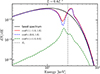 |
Fig. 2. Representative emergent spectrum for an XRP with a fiducial luminosity L = 0.6L*. The solid black line represents the seed blackbody spectrum with temperature kBT = 5.9 keV. The solid red line shows the total normalized emergent spectrum. The dashed blue and green lines correspond to the angle-selected spectra observed at polar angles in the ranges (0, π/2) and (π/2, π), respectively. The vertical dashed gray line indicates the cyclotron energy at Ec = 25.55 keV. The spectrum features a redshifted, but prominent CRSF around E ∼ 20 keV followed by a bump. The angle-selected spectra are scaled relative to their contribution to the total photon flux. |
The CRSF appears redshifted with respect to the local cyclotron energy. The origin of this shift is related to the Doppler effect between the lab frame and the electron’s bulk rest frame, as described qualitatively in Sect. 2.2. We discuss this effect in more detail in the following paragraphs.
Furthermore, we note that the dominant contribution to the total flux arises from photons escaping at angles in the range (0, π/2), owing to the low optical depth values away from resonance and the reflection (or thermalization) of photons crossing the base of the funnel. Yet, a minor fraction of photons escape toward the NS surface. The spectrum of this latter population does not exhibit a prominent absorption feature at the energies corresponding to the CRSF in the total spectrum, since photons propagating with cos θ < 0 are typically out of resonance at those energies. Instead, an absorption feature appears at higher energies, where photons are in resonance with the electrons, but it is strongly smeared out by the contribution of red- and blue-wing photons propagating in different directions. Escaped photons directed toward the NS will likely be reflected off the surface; however, their contribution to the total spectrum is negligible. We therefore safely neglected this photon population and the associated modeling of surface reflection outside the funnel.
To further illuminate the formation of the CRSF, we investigated the angular dependence of the emergent spectrum, which is relevant for phase-resolved studies of CRSFs. Fig. 3 shows the total spectrum in the range (0, π/2) in black, along with decomposed into five narrow viewing angle bins spectra in various colors. We note that the choice of the number of angular bins was arbitrary and does not affect the conclusions. The angle-dependent spectra were scaled based on their relative contribution in the photon flux. For convenience, the position of the classical cyclotron energy is also marked by a dashed vertical gray line.
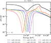 |
Fig. 3. Angle-resolved spectra for a typical XRP source with luminosity L = 0.6L*. The solid black line corresponds to the angle-averaged spectrum in the range (0, π/2). The dashed colored lines show spectra extracted in five angular bins within this range. Each spectrum has been normalized to its angular flux contribution. The vertical gray line marks the local cyclotron energy. With increasing cos θ, the CRSF centroid energy shifts to lower values and the blue wing becomes more pronounced. |
Evidently, the CRSF profile and its wings depend strongly on the viewing angle, exhibiting two primary characteristics. First, the centroid energy of the CRSF decreases with increasing cos θ. Specifically, as cos θ approaches zero (corresponding to directions perpendicular to the z-axis), the redshift relative to Ec becomes smaller. This behavior arises from the Doppler effect discussed in Sect. 2.2. A photon propagating at an angle θ with respect to the z-axis is in resonance with the infalling electrons when its energy is approximately Ec/γ(1 + β cos θ) (see Eq. (14)); thus, larger values of cos θ correspond to lower resonant energies, naturally producing the trend shown in Fig. 3.
Second, the blue wing becomes increasingly prominent and shifts to higher energies as cos θ increases. This behavior is a direct consequence of the implementation of the reflection scheme: Seed photons undergoing resonant scattering acquire their maximum energies when they are backscattered and therefore Doppler beamed toward the stellar surface (i.e., at angles near cos θ ≈ −1). Upon reflection from the base of the funnel, these high-energy photons reemerge at viewing angles near cos θ ≈ 1, manifesting as prominent blue wings.
Finally, we find that the angle-averaged spectrum features a broader, asymmetric, but shallower CRSF compared to those in angle-resolved spectra. The superposition of CRSFs formed at different viewing angles–each centered at a slightly different energy–produces a wider and shallower feature due to the partial overlap of individual absorption profiles with the wings of neighboring lines. At low luminosity, this is very prominent (see Appendix B).
4.2. Variability due to the accretion luminosity
Having studied the angular dependence of the CRSF properties and the physical origin of the associated spectral features, we now turn to their dependence on the accretion luminosity. At higher luminosities, the braking of the infalling plasma becomes more efficient; consequently, the Doppler effect, which causes the cyclotron energy to appear redshifted, is reduced. As a result, we expect the centroid energy to lie closer to the local value Ec at higher luminosities (see also Sect. 2.2).
We performed a total of 11 simulations, varying the accretion luminosity while keeping all other model parameters fixed. Figure 4 displays the angle-averaged emergent spectra for different luminosities, with the inset highlighting the energy range around the CRSF. All spectra are normalized to unity. As anticipated, the CRSF centroid energy shifts systematically toward higher energies with increasing luminosity, establishing a positive correlation between L and ECRSF (for a quantitative characterization, see Sect. 4.3), in agreement with the predictions of Mushtukov et al. (2015b).
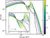 |
Fig. 4. Angle-averaged emergent spectra for luminosities spanning the range L/L* ∈ (0, 1). The color gradient from dark blue to yellow corresponds to increasing luminosity. The inset highlights the spectral region around the CRSF. The vertical gray dashed line denotes the local cyclotron energy. The positive correlation between L and the CRSF energy ECRSF is evident. |
In addition, the blue wing becomes increasingly pronounced and the CRSF deepens with increasing luminosity. The overall spectrum also hardens. Higher luminosities correspond to larger plasma number densities (and thus optical depth), as Eq. (7) suggests, due to (i) an increased accretion rate and (ii) enhanced compression associated with a reduced terminal velocity. The resulting increase in optical depth naturally accounts for the deepening of the CRSF, the strengthening of the blue wing, and the observed spectral hardening.
4.3. Phase-dependent variability of the line features
Having demonstrated the strong variability of the CRSF with luminosity (Sect. 4.2) and viewing angle (Sect. 4.1), we now quantify the dependence of the line centroid energy ECRSF and width σCRSF on these two parameters. Figure 5a displays the CRSF centroid energy as a function of luminosity for five angular intervals spanning the range (0, π/2), together with the values measured from the angle-averaged spectra in black. We defined ECRSF as the centroid of the CRSF after subtracting the underlying continuum (see Appendix C). A clear positive correlation between ECRSF and luminosity is present for all viewing angles, as well as for angle-averaged spectra.
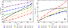 |
Fig. 5. Dependence of the CRSF centroid energy ECRSF (panel a) and width σCRSF (panel b) on luminosity and viewing angle θ (measured with respect to the magnetic axis). Results are shown for five angular bins spanning the range θ ∈ (0, π/2), with Ec = 25.55 keV. Solid black lines denote quantities extracted from angle-averaged spectra. Both ECRSF and σCRSF exhibit a positive correlation with luminosity for all viewing angles. At a fixed luminosity, ECRSF (σCRSF) decreases (increases) toward smaller viewing angles, indicating substantial variability over the pulse cycle. |
At a fixed luminosity, the centroid energy varies systematically with viewing angle: smaller angles relative to the z-axis (i.e., face-on views of the hotspot) consistently yield lower values of ECRSF, indicating an anticorrelation with cos θ. An explanation is given in Sect. 4.1. The amplitude of this angular variation is ∼30% at low luminosities and decreases as the luminosity increases. From Eq. (14), the resonant energy range of photons moving away from the star spans [ECRSF(θ = 0),ECRSF(θ = π/2)], that is
![Mathematical equation: $$ \begin{aligned} \dfrac{\Delta E|_{\rm CRSF}}{E_{\rm res}} \approx \dfrac{1}{\gamma } - \dfrac{1}{\gamma ( 1 + \beta )} = [\gamma (1 + 1/\beta )]^{-1}. \end{aligned} $$](/articles/aa/full_html/2026/05/aa59285-26/aa59285-26-eq40.gif) (33)
(33)
Substituting β with the terminal velocity β0, we get ΔE|CRSF/Eres ≈ 29% for β0 = 0.5, which corresponds to L ≪ L*. At higher luminosities, β0 decreases (Eq. (5)), leading to a smaller ΔE|CRSF, in agreement with the simulation results.
Figure 5b is analogous to Fig. 5a, but shows the CRSF width. While several definitions of line width exist, depending on the assumed profile, here we characterized σCRSF as the full width at half minimum (FWHM) of the CRSF after subtracting the underlying continuum; for details we refer the reader to Appendix C. We find that the line width increases with luminosity for all viewing angles, although its absolute value depends substantially on θ. The widths corresponding to the angle-averaged spectra (black curve) are systematically higher than those in angle-dependent spectra, as the width in the former case is dominated by the superposition of CRSFs forming at different angles (see Figs. 3 and B.1). In addition, we find that σCRSF is positively correlated with cos θ, in agreement with the predictions of Mushtukov et al. (2015b).
This behavior can be easily understood qualitatively as follows. Higher luminosities produce stronger radiative drag, resulting in a steeper velocity gradient in the accretion flow (see Eq. (3)). Photons traversing the funnel therefore sample a broader range of electron bulk velocities, leading to increased Doppler broadening of the CRSF and a positive correlation between σCRSF and L. For a given velocity profile (i.e., fixed luminosity), the magnitude of this effect depends on the propagation direction relative to the flow (in this case, the z-axis): smaller values of cos θ suppress Doppler shifts (see Eq. (14)), while the maximum broadening occurs for photons propagating nearly parallel to the magnetic (flow) axis, cos θ ≈ 1.
Taken together, these results imply that both the CRSF centroid energy and width increase with luminosity, such that higher values of ECRSF are accompanied by broader lines. Consequently, in studies of phase-averaged spectral evolution, this model predicts a correlated increase of the CRSF energy and width with luminosity. Conversely, the trend reverses for short-timescale, phase-resolved variability. As shown above, ECRSF anticorrelates with cos θ, whereas σCRSF correlates positively with cos θ. For a given luminosity, therefore, the model yields an anticorrelation between the CRSF energy and width. Over a pulse cycle, the line energy (width) reaches its minimum (maximum) value when the accretion funnel is viewed face-on, i.e., along the magnetic-field direction, and its maximum (minimum) when it is seen edge-on.
5. Comparison with data: An application to the X-ray pulsar GX 304−1
Following Mushtukov et al. (2015b), we tested our model by applying it to the observed CRSF variability in the X-ray pulsar GX 304−1, a source exhibiting well-established ECRSF − L and σCRSF − L positive correlations (Klochkov et al. 2012). We adopted the CRSF centroid energy and width measurements reported by Mushtukov et al. (2015b), who analyzed INTEGRAL (Winkler et al. 2003) observations of GX 304−1 obtained during the 2012 type-II outburst (Yamamoto et al. 2012).
To facilitate a direct comparison with the data, we performed an additional set of MC simulations employing the reflection scheme, as described in Sect. 4, but, following Mushtukov et al. (2015b), we took the classical cyclotron energy to be  , corresponding to a dimensionless magnetic field strength of b ≈ 0.13, and adopted a critical luminosity of LGX* = 2.7 × 1037 erg s−1. The remaining dimensionless NS parameters used in this exercise are listed in Table 2. The photon injection protocol was identical to that utilized in runs shown in Sect. 4.
GX 304-1 model parameters.
Figures 6a and b show the GX 304−1 data (red and black circles) together with our simulation results (colored lines) for ECRSF (left panel) and σCRSF (right panel) as functions of luminosity, for three representative narrow viewing-angle intervals. We measured ECRSF and σCRSF from the simulated spectra as described in Sect. 4.3. Regarding the data, black circles correspond to CRSF parameters inferred using a Gaussian absorption profile (GABS), while red circles denote results obtained using a Lorentzian profile (CYCLABS). Further details concerning the data analysis can be found in Sect. 3 of Mushtukov et al. (2015b).
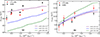 |
Fig. 6. Comparison of observed cyclotron line variability in GX 304-1 with our model. Panel a (b) shows the CRSF centroid energy (width). Red and black circles represent the observed ECRSF and σCRSF values of GX 304-1, obtained using the CYCLABS model (Lorentzian profile) and the GABS model (Gaussian profile), respectively, to fit the line feature (Mushtukov et al. 2015b). Green, blue, and purple lines correspond to the results derived from our MC simulations for three different viewing angle intervals. The model predictions, for specific viewing angles, agree sufficiently well with the data over an order of magnitude in luminosity. |
The model successfully reproduces the observed trends and, for fixed viewing angles, provides good agreement with the data over nearly an order of magnitude in luminosity. In particular, viewing angles corresponding to cos θ ∈ (0.0 − 0.1) (purple curves) simultaneously match both the CRSF centroid energy and width, whereas larger values of cos θ are inconsistent with one or both observables. Since the viewing angle is primarily governed by the system geometry (neglecting gravitational light bending, which is not included here), this result favors configurations in which the accretion funnel (and thus the hotspot) is viewed predominantly edge-on over the pulse cycle. Such configurations may correspond either to a near-orthogonal rotator (α ∼ 70° −90°) observed at low inclination (i ∼ 0° −20°), or to a near-aligned rotator (α ∼ 0° −20°) observed at high inclination (i ∼ 70° −90°). Here, i denotes the angle between the line of sight and the rotation axis, and α is the inclination of the magnetic axis relative to the rotation axis. The latter scenario is the one proposed by Mushtukov et al. (2015b), based on phase-averaged modeling of the CRSF variability, and is consistent with our findings.
Nevertheless, it would be premature to use this comparison to place quantitative constraints on the physical parameters of GX 304−1. Our analysis does not include phase averaging over the pulse cycle, nor does it account for general-relativistic light bending. Additional limitations arise from parameter degeneracies inherent to our modeling approach, including the assumed values of  , LGX*, and other NS parameters. For instance, adopting a higher value of
  would favor larger values of cos θ in order to maximize the Doppler redshift, potentially altering the inferred geometry. Likewise, increasing βff would steepen the predicted ECRSF − L correlation. A comprehensive comparison with the data therefore requires treating all relevant model parameters as free and performing full phase-averaged calculations, which we defer to future work.
6. Discussion and conclusions
In this work, we investigated quantitatively the origin of the CRSF variability observed in subcritical (L ≲ L*) XRPs by means of resonant scattering in the accretion funnel above the hotspot, following the model proposed by Mushtukov et al. (2015b). We focused on two key spectral properties: the positive correlations of the CRSF centroid energy, ECRSF, and line width, σCRSF, with the X-ray luminosity, L.
We developed a relativistic MC code, based on the framework described by Loudas et al. (2024b), to perform detailed radiative-transfer calculations in the accretion funnel and derive emergent, angle-dependent spectra. For simplicity, we assumed a semi-infinite cylindrical accretion channel above the hotspot, centered on the magnetic axis. Seed blackbody radiation was injected isotropically upward from the hotspot. The accretion flow was taken to be cold, while the plasma density and velocity profiles were computed analytically, capturing the effects of radiation pressure.
The primary model parameters governing our calculations were the critical luminosity L* and the surface magnetic field strength B. Other free parameters – such as the NS mass, NS radius, and free-fall speed – were fixed to fiducial values. We varied the accretion luminosity L over a wide range to study its impact on the CRSF properties. As a proof-of-concept, we applied our model to observational data of the X-ray pulsar GX 304−1.
Our main conclusions can be summarized as follows:
-
Resonant scattering of hotspot radiation by the accretion flow imprints a prominent CRSF, followed by a broad blue wing (Fig. 1). The CRSF is always redshifted relative to the local cyclotron energy, Ec, due to the Doppler effect; the magnitude of the redshift decreases both at higher luminosities (Fig. 4) and at larger viewing angles relative to the magnetic axis (Fig. 3).
-
The CRSF centroid energy and width are positively correlated with luminosity for all viewing angles (Fig. 5), reflecting changes in the accretion-flow velocity profile, although their absolute values vary across viewing angles. With increasing luminosity, the blue wing becomes increasingly pronounced, the CRSF deepens, and the overall spectrum hardens due to the increase in the optical depth (Fig. 4).
-
The CRSF properties exhibit strong variability over the pulse cycle. At a fixed luminosity, ECRSF (σCRSF) decreases (increases) with cos θ; the centroid energy reaches its maximum when the funnel is viewed edge-on due to the suppression of the Doppler shift. In contrast, the line width is maximized when the funnel is viewed face-on, as photons sample a broader range of bulk velocities. Thus, in phase-resolved studies, ECRSF anticorrelates with σCRSF during the pulse cycle (Fig. 5).
-
Angle-averaged spectra feature broader, asymmetric, but shallower CRSFs compared to angle-resolved spectra (i.e., at a given pulse phase), owing to the superposition of CRSFs formed at different viewing angles (Fig. 3).
-
When applied to the observational data of the X-ray pulsar GX 304−1, the model successfully reproduces the observed variability of the CRSF centroid energy and width over nearly an order of magnitude in luminosity (Fig. 6). In particular, configurations in which the accretion channel is predominantly viewed edge-on are favored, in line with Mushtukov et al. (2015b), providing tentative constraints on the viewing geometry of the system (see Sect. 5).
Our findings are consistent with the qualitative predictions of Mushtukov et al. (2015b), supporting the hypothesis that the accretion channel constitutes the line-forming region and that the flow velocity profile drives the observed variability. However, unlike those predictions, which rely solely on the behavior of the resonant optical depth, our calculations self-consistently incorporate key radiative-transfer effects, such as photon energy redistribution during scattering, which is responsible for the formation of the CRSF wings.
While the model captures the essential physics governing CRSF variability in subcritical XRPs and successfully reproduces well-established observational trends, it relies on a number of simplifying assumptions that introduce limitations and motivate future extensions. First, we assumed a simplified cylindrical, filled accretion channel; however, more realistic magnetospheric flows point to bow-shaped or annular footprints (see, e.g., Zhu 2025, and references therein), which, nevertheless, we do not expect to alter our conclusions. Second, the funnel was extended to infinity, neglecting the global magnetospheric accretion picture, and assuming a constant magnetic field strength. Neither assumption is physical; however, as we argued in Sect. 2.2, the accretion flow is optically thick to resonant scattering; therefore, the line-forming region lies above the hotspot and is relatively compact. Considering a dipole field (B(r)∝r−3) and a vertical size of the line-forming region comparable to the hotspot size (Eq. (4)), the expected variation due to the magnetic field gradient is ≲(3 − 6)%.
We employed analytical, one-dimensional velocity and density profiles; however, RMHD simulations (Markozov et al. 2023) reveal more complex profiles, as the effect of radiation pressure force is less effective near the edges of the funnel, where radiation can easily escape sideways. This subtlety might affect the exact CRSF shape and slope of predicted correlations, but it would not change our conclusions. In addition, we treated the accretion flow as cold (i.e., kBTe ≪ Ec). We expect the electron’s temperature to modify the CRSF shape through thermal broadening. So, this approximation is valid, so long as the Doppler effect and the velocity gradient govern the CRSF width. In Sect. 4, we showed that for a typical cyclotron line energy of Ec ≈ 25 keV, σCRSF is always greater than 2 keV. Therefore, for electron temperatures of kBTe ≲ 2 keV, thermal effects will likely not be important.
Our model does not include a detailed description of the NS atmosphere beneath the accretion funnel (i.e., z < 0) or the associated physical processes. To assess the sensitivity of our results to the treatment of the lower boundary, we considered two limiting cases: one in which photons reaching the base undergo geometric reflection (reflection scheme), conserving their energy, and another in which photons get absorbed and reemitted as blackbody radiation (thermalization scheme). We find that our primary conclusions regarding the CRSF variability are robust against the choice of boundary condition. Additionally, as discussed in Sect. 4.1, we neglected the reflection of downward-escaping photons off the NS surface outside the accretion funnel, as their contribution to the total emergent spectrum is negligible. Nevertheless, a more physically motivated treatment that self-consistently accounts for the structure, plasma dynamics, and radiative transfer in the NS atmosphere – as well as the surrounding stellar surface – would further strengthen the predictive power of the model. Such an extension is beyond the scope of the present work and is left for future explorations.
Another simplification in our calculations concerns the treatment of the hotspot emission. We assumed isotropic, upward blackbody emission, uniformly from the base of the accretion funnel. In contrast, more detailed hotspot emission models predict anisotropic, Comptonized spectra (see, e.g., Meszaros & Nagel 1985; Sokolova-Lapa et al. 2021). To assess the sensitivity of our results to this assumption, we tested alternative emission prescriptions, including pencil-like patterns and point-source emission centered at the origin, (0, 0, 0). In all cases, the resulting variations in the CRSF centroid energy and width were at ≲10% level. This indicates that the CRSF variability explored in this work is not strongly sensitive to the assumed hotspot emission pattern, although we expect such effects to play a critical role in the modeling of pulse profiles, which we will explore in future work.
In this work, we performed polarization-independent calculations. With the current (IXPE Weisskopf et al. 2022; XL-Calibur Abarr et al. 2021; XPoSat1) and upcoming (eXTP Zhang et al. 2025b) X-ray polarimetry missions, polarization data are becoming increasingly available. X-ray polarization holds strong constraining power regarding the system’s geometry (Poutanen et al. 2024); thus, incorporating polarization into our radiative transfer scheme is a vital next step. We plan to address this topic in detail in our forthcoming work.
Finally, we neglected general relativistic effects in this analysis, which can be important for pulse-profile modeling and thorough comparisons with observations (see, e.g., Markozov & Mushtukov 2024). Such effects may influence our results through: (i) gravitational redshift of the CRSF energy and width, as well as the inferred luminosity, and (ii) gravitational lensing by the NS. While gravitational redshift may shift the absolute values of the CRSF parameters, we expect this shift to be nearly identical in all cases, since the extent of the line-forming region above the hotspot is small. Thus, it should not affect the variability of the CRSF dramatically. Similarly, gravitational light bending will modify the observed range of viewing angles and introduce contributions from the antipodal hotspot. We expect these effects to become important when constructing the predicted pulse profiles.
An alternative interpretation of CRSF variability in subcritical XRPs is provided by the CS scenario, which identifies the line formation site as the region between the hotspot and the shock front. In this framework, the observed variations in the CRSF energy and width are attributed to changes in the local magnetic field strength at the line-forming region, which are tied to the shock altitude. When applied to the GX 304−1 system, this model successfully reproduces the luminosity dependence of the CRSF properties in phase-averaged spectra (Rothschild et al. 2017). Because bulk motion effects in the post-shock region are negligible, the CS model does not predict pulse-resolved CRSFs to exhibit strong variability with the pulse phase (i.e., viewing angle), in contrast to the scenario explored in this work. This fundamental difference between the two models offers a potential observational discriminant that could help distinguish between competing interpretations and advance our understanding of cyclotron line formation in subcritical XRPs. However, such a test requires the development of a robust model for the shock structure, followed by self-consistent radiative-transfer calculations.
In summary, building on the framework proposed by Mushtukov et al. (2015b), we have demonstrated a plausible physical origin of key observational trends in subcritical X-ray pulsars, including the luminosity- and phase-dependent variability of cyclotron lines, by means of resonant scattering in the accretion funnel. Our results highlight the central role of bulk motion in shaping the CRSF properties and provide new insights into the dynamics and geometry of the accretion flow.
Data availability
The results presented in this paper were obtained using a proprietary code developed by the authors. The data supporting the figures, as well as the code, are available from the corresponding author upon reasonable request.
Acknowledgments
We thank the referee for their careful reading of the manuscript and for their constructive comments that helped improve the clarity of this work. PF thanks Chryssi Koukouraki and Orestis Zoumpoulakis (Institute of Astrophysics, Foundation for Research and Technology-Hellas) for their technical assistance. NL acknowledges support from the Venture Forward Fellowship of the Department of Astrophysical Sciences at Princeton University. NL thanks Lizhong Zhang for valuable discussions on accretion column dynamics, and Anatoly Spitkovsky for insightful discussions on the underlying physics of the collisionless shock scenario as an accretion-halting mechanism above the hotspot.
References
- Abarr, Q., Awaki, H., Baring, M. G., et al. 2021, Astropart. Phys., 126, 102529 [Google Scholar]
- Araya, R. A., & Harding, A. K. 1999, ApJ, 517, 334 [NASA ADS] [CrossRef] [Google Scholar]
- Arons, J., Klein, R. I., & Lea, S. M. 1987, ApJ, 312, 666 [Google Scholar]
- Basko, M. M., & Sunyaev, R. A. 1975, A&A, 42, 311 [NASA ADS] [Google Scholar]
- Basko, M. M., & Sunyaev, R. A. 1976, MNRAS, 175, 395 [Google Scholar]
- Becker, P. A., & Wolff, M. T. 2005, ApJ, 630, 465 [NASA ADS] [CrossRef] [Google Scholar]
- Becker, P. A., & Wolff, M. T. 2007, ApJ, 654, 435 [NASA ADS] [CrossRef] [Google Scholar]
- Becker, P. A., Klochkov, D., Schönherr, G., et al. 2012, A&A, 544, A123 [NASA ADS] [CrossRef] [EDP Sciences] [Google Scholar]
- Bisnovatyi-Kogan, G. S., & Fridman, A. M. 1970, Sov. Astron., 13, 566 [NASA ADS] [Google Scholar]
- Burnard, D. J., Arons, J., & Klein, R. I. 1991, ApJ, 367, 575 [CrossRef] [Google Scholar]
- Bykov, A. M., & Krasil’Shchikov, A. M. 2004, Astron. Lett., 30, 309 [NASA ADS] [CrossRef] [Google Scholar]
- Canuto, V., Lodenquai, J., & Ruderman, M. 1971, Phys. Rev. D, 3, 2303 [NASA ADS] [CrossRef] [Google Scholar]
- Chen, X., Wang, W., Tang, Y. M., et al. 2021, ApJ, 919, 33 [CrossRef] [Google Scholar]
- Fürst, F., Falkner, S., Marcu-Cheatham, D., et al. 2018, A&A, 620, A153 [NASA ADS] [CrossRef] [EDP Sciences] [Google Scholar]
- Ghosh, P., & Lamb, F. K. 1978, ApJ, 223, L83 [Google Scholar]
- Ghosh, P., & Lamb, F. K. 1979, ApJ, 232, 259 [Google Scholar]
- Gnedin, I. N., & Sunyaev, R. A. 1974, A&A, 36, 379 [NASA ADS] [Google Scholar]
- Gonthier, P. L., Baring, M. G., Eiles, M. T., et al. 2014, Phys. Rev. D, 90, 043014 [NASA ADS] [CrossRef] [Google Scholar]
- Harding, A. K., & Daugherty, J. K. 1991, ApJ, 374, 687 [NASA ADS] [CrossRef] [Google Scholar]
- Klein, R. I., Arons, J., Jernigan, G., & Hsu, J. J.-L. 1996, ApJ, 457, L85 [Google Scholar]
- Klochkov, D., Doroshenko, V., Santangelo, A., et al. 2012, A&A, 542, L28 [NASA ADS] [CrossRef] [EDP Sciences] [Google Scholar]
- Kumar, S., Bala, S., & Bhattacharya, D. 2022, MNRAS, 515, 914 [CrossRef] [Google Scholar]
- Kylafis, N. D., Trümper, J. E., & Loudas, N. A. 2021, A&A, 655, A39 [NASA ADS] [CrossRef] [EDP Sciences] [Google Scholar]
- Landau, L. 1930, Z. Phys., 64, 629 [NASA ADS] [CrossRef] [Google Scholar]
- Langer, S. H., & Rappaport, S. 1982, ApJ, 257, 733 [NASA ADS] [CrossRef] [Google Scholar]
- Loudas, N., Kylafis, N. D., & Trümper, J. 2024a, A&A, 689, A75 [NASA ADS] [CrossRef] [EDP Sciences] [Google Scholar]
- Loudas, N., Kylafis, N. D., & Trümper, J. 2024b, A&A, 685, A95 [NASA ADS] [CrossRef] [EDP Sciences] [Google Scholar]
- Loudas, N. A., Kylafis, N. D., & Trümper, J. E. 2021, A&A, 655, A38 [NASA ADS] [CrossRef] [EDP Sciences] [Google Scholar]
- Malacaria, C., Klochkov, D., Santangelo, A., & Staubert, R. 2015, A&A, 581, A121 [NASA ADS] [CrossRef] [EDP Sciences] [Google Scholar]
- Maniadakis, D. K., Sokolova-Lapa, E., D’Aì, A., et al. 2025, A&A, 700, A70 [NASA ADS] [CrossRef] [EDP Sciences] [Google Scholar]
- Markozov, I. D., Kaminker, A. D., & Potekhin, A. Y. 2023, Astron. Lett., 49, 583 [CrossRef] [Google Scholar]
- Markozov, I. D., & Mushtukov, A. A. 2024, MNRAS, 527, 5374 [Google Scholar]
- Meszaros, P., & Nagel, W. 1985, ApJ, 298, 147 [NASA ADS] [CrossRef] [Google Scholar]
- Miller, G. S., Salpeter, E. E., & Wasserman, I. 1987, ApJ, 314, 215 [Google Scholar]
- Mushtukov, A., & Tsygankov, S. 2022, in Accreting Strongly Magnetized Neutron Stars: X-ray Pulsars, eds. C. Bambi, & A. Santangelo (Singapore: Springer Nature), 1 [Google Scholar]
- Mushtukov, A. A., Suleimanov, V. F., Tsygankov, S. S., & Poutanen, J. 2015a, MNRAS, 447, 1847 [NASA ADS] [CrossRef] [Google Scholar]
- Mushtukov, A. A., Tsygankov, S. S., Serber, A. V., Suleimanov, V. F., & Poutanen, J. 2015b, MNRAS, 454, 2714 [Google Scholar]
- Mushtukov, A. A., Nagirner, D. I., & Poutanen, J. 2016, Phys. Rev. D, 93, 105003 [Google Scholar]
- Mushtukov, A. A., Suleimanov, V. F., Tsygankov, S. S., & Portegies Zwart, S. 2021, MNRAS, 503, 5193 [Google Scholar]
- Nobili, L., Turolla, R., & Zane, S. 2008, MNRAS, 389, 989 [NASA ADS] [CrossRef] [Google Scholar]
- Poutanen, J., Mushtukov, A. A., Suleimanov, V. F., et al. 2013, ApJ, 777, 115 [NASA ADS] [CrossRef] [Google Scholar]
- Poutanen, J., Tsygankov, S. S., & Forsblom, S. V. 2024, Galaxies, 12, 46 [NASA ADS] [CrossRef] [Google Scholar]
- Romanova, M. M., Ustyugova, G. V., Koldoba, A. V., & Lovelace, R. V. E. 2004, ApJ, 610, 920 [Google Scholar]
- Rothschild, R. E., Kühnel, M., Pottschmidt, K., et al. 2017, MNRAS, 466, 2752 [Google Scholar]
- Roy, K., & Sharma, R. 2025, New Astron., 121, 102435 [Google Scholar]
- Santangelo, A., Segreto, A., Giarrusso, S., et al. 1999, ApJ, 523, L85 [NASA ADS] [CrossRef] [Google Scholar]
- Schwarm, F. W., Schönherr, G., Falkner, S., et al. 2017, A&A, 597, A3 [NASA ADS] [CrossRef] [EDP Sciences] [Google Scholar]
- Shui, Q. C., Zhang, S., Wang, P. J., et al. 2024, MNRAS, 528, 7320 [NASA ADS] [CrossRef] [Google Scholar]
- Sina, R. 1996, Ph.D. Thesis, University of Maryland, College Park [Google Scholar]
- Sokolova-Lapa, E., Gornostaev, M., Wilms, J., et al. 2021, A&A, 651, A12 [NASA ADS] [CrossRef] [EDP Sciences] [Google Scholar]
- Staubert, R., Shakura, N. I., Postnov, K., et al. 2007, A&A, 465, L25 [NASA ADS] [CrossRef] [EDP Sciences] [Google Scholar]
- Staubert, R., Klochkov, D., Fürst, F., et al. 2017, A&A, 606, L13 [NASA ADS] [CrossRef] [EDP Sciences] [Google Scholar]
- Staubert, R., Trümper, J., Kendziorra, E., et al. 2019, A&A, 622, A61 [NASA ADS] [CrossRef] [EDP Sciences] [Google Scholar]
- Truemper, J., Pietsch, W., Reppin, C., et al. 1978, ApJ, 219, L105 [CrossRef] [Google Scholar]
- Trümper, J., Pietsch, W., Reppin, C., et al. 1977, Mitteilungen der Astronomischen Gesellschaft Hamburg, 42, 120 [Google Scholar]
- Tsygankov, S. S., Lutovinov, A. A., Churazov, E. M., & Sunyaev, R. A. 2006, MNRAS, 371, 19 [NASA ADS] [CrossRef] [Google Scholar]
- Tsygankov, S. S., Lutovinov, A. A., & Serber, A. V. 2010, MNRAS, 401, 1628 [NASA ADS] [CrossRef] [Google Scholar]
- Ventura, J. 1979, Phys. Rev. D, 19, 1684 [Google Scholar]
- Vybornov, V., Klochkov, D., Gornostaev, M., et al. 2017, A&A, 601, A126 [NASA ADS] [CrossRef] [EDP Sciences] [Google Scholar]
- Weisskopf, M. C., Soffitta, P., Baldini, L., et al. 2022, J. Astron. Telesc. Instrum. yst., 8, 026002 [Google Scholar]
- Weng, S.-S., & Ji, L. 2024, Universe, 10, 453 [Google Scholar]
- Winkler, C., Courvoisier, T. J.-L., Di Cocco, G., et al. 2003, A&A, 411, L1 [NASA ADS] [CrossRef] [EDP Sciences] [Google Scholar]
- Xiao, G. C., Ji, L., Staubert, R., et al. 2019, JHEAp, 23, 29 [Google Scholar]
- Yamamoto, T., Tomida, H., Mihara, T., et al. 2012, ATel, 3856, 1 [NASA ADS] [Google Scholar]
- Yang, W., Wang, W., Liu, Q., et al. 2023, MNRAS, 519, 5402 [NASA ADS] [CrossRef] [Google Scholar]
- Zel’dovich, Y. B., & Shakura, N. I. 1969, Sov. Astron., 13, 175 [NASA ADS] [Google Scholar]
- Zhang, L., Blaes, O., & Jiang, Y.-F. 2022, MNRAS, 515, 4371 [NASA ADS] [CrossRef] [Google Scholar]
- Zhang, L., Blaes, O., & Jiang, Y.-F. 2023, MNRAS, 520, 1421 [CrossRef] [Google Scholar]
- Zhang, L., Blaes, O., & Jiang, Y.-F. 2025a, MNRAS, 540, 3934 [Google Scholar]
- Zhang, S.-N., Santangelo, A., Xu, Y., et al. 2025b, Sci. China Phys. Mech. Astron., 68, 119502 [Google Scholar]
- Zhu, Z. 2025, MNRAS, 537, 3701 [Google Scholar]
Appendix A: Boundary effects
In this appendix, we investigate the effect of the boundary condition at the base of the accretion column on the CRSF properties. To do so, we repeated the calculations presented in Sect. 4, using the thermalization scheme instead of the reflection scheme. Specifically, photons hitting the base of the accretion column are not reflected back; rather, they are absorbed and reemitted as seed photons, following the initial blackbody distribution. We expect this change to modify the shape of the line wings, but not the centroid position, as the scattering mechanism remains the same. In particular, we expect an enhancement of the red wing, as each time a photon packet reaches the base, its energy is resampled and kBT < Ec. This process effectively removes photons from the blue wing and redistributes them to the left of the absorption line.
In Fig. A.1, we compare the angle-averaged spectra obtained using the two different boundary conditions for luminosity L = 0.6L*. It is evident that when the thermalization scheme is implemented (blue line), the red wing dominates over the blue one, whereas for the reflection scheme (red line), the opposite is observed. However, the position of the absorption line is the same in both cases; the centroid energy of the CRSF is insensitive to the boundary condition.
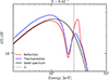 |
Fig. A.1. Comparison of angle-averaged spectra with different boundary conditions for a typical source with luminosity L = 0.6L* and Ec = 25.55 keV (vertical gray dashed line). The solid black line represents the seed blackbody spectrum with kBT = 5.9 keV. The solid red (blue) line shows the emergent spectrum for the reflection (thermalization) case. The line wings exhibit differences; the red (blue) wing dominates in the thermalization (reflection) scheme. The centroid energy of the CRSF appears to be independent of the boundary condition. |
In analogy with Fig. 4, Fig. A.2 shows the resulting spectra for 11 different luminosities L. The positive correlation between the position of the CRSF and luminosity is again evident. The thermalization scheme suppresses the blue wing and enhances the red wing, as described qualitatively above. Even at high luminosities, the blue wing remains relatively weak.
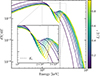 |
Fig. A.2. Same as Fig. 4, but for the thermalization scheme. The luminosity dependence of the CRSF properties is the same. |
Figure A.3 is the same as Fig. 5, but also includes the results obtained using the thermalization scheme in triangles connected with dashed lines. From Fig. A.3a, it is evident that the centroid energy is not affected by the scheme used, regardless of the luminosity and/or viewing angle.
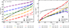 |
Fig. A.3. Same as Fig. 5, but including the results obtained using the thermalization scheme in triangles connected with dashed lines. While the energy of the cyclotron feature is independent of the boundary scheme, the line width shows deviations at high luminosities. We expect this, as the redistribution of photons into the line wings alters the CRSF shape, affecting its width. |
In contrast, the line width is sensitive to the overall shape of the absorption feature, including its wings; consequently, we expect differences between the two schemes. This is apparent in Fig. A.3b, where the results for the two schemes diverge at luminosities L ≳ 0.5L*. The discrepancy between the dashed (thermalization) and solid (reflection) lines increases with luminosity and is most pronounced at small values of cos θ. The primary cause of this divergence is the effective narrowing of the CRSF in the reflection scheme due to its prominent blue wing, which is absent in the thermalization case (see Figs. A.1 and A.2). We note, however, that the quantitative determination of the line width is subject to systematic uncertainties. The derived values depend heavily on the modeling of the underlying continuum and the choice of line profile (e.g., Gaussian or Lorentzian).
Appendix B: Absorption feature at low luminosity
This appendix aims at explaining the lack of a prominent absorption feature in the spectrum at low luminosities in our simulations. To this end, in Fig. B.1 we present the angle-resolved spectrum for a low luminosity value, L = 0.1L*, calculated using the reflection scheme. All features seen in Fig. 3 are present here as well: the centroid energy is anti-correlated with cos θ, and the blue wing becomes increasingly prominent and shifts to higher energies as cos θ increases. However, in contrast to the L = 0.6L* case, the superposition of lines emerging at different viewing angles in the low luminosity regime results in a shallow, almost flat CRSF, making it a challenging task to accurately identify the angle-averaged CRSF centroid. Nevertheless, the feature is readily distinguishable after subtraction of the underlying continuum, enabling a reliable determination of the centroid energy.
Appendix C: Calculation of line parameters
This appendix outlines the methodology used to measure the relevant CRSF parameters: the centroid energy (ECRSF) and the line width (σCRSF). The CRSF shape is rather complicated, asymmetric, and deviates significantly from a Gaussian or a Lorentzian profile; thus, we adopted an approach that allows for a robust metric without any bias introduced by fitting specific analytical profiles. We defined the centroid energy as the flux-weighted average energy in the vicinity of the local minimum, and the line width as the full width at half minimum (FWHM) of the absorption feature’s depth.
Figure C.1 illustrates our approach, showing its implementation in a representative angle-averaged spectrum (cos θ ∈ (0, 1)) for a source with luminosity L = 0.6L*, computed using the thermalization scheme. To estimate the line parameters, we first subtracted the background blackbody continuum (SBB; black dashed line) from the total emergent spectrum (Stot; solid gray line). Since the resulting residual spectrum (Stot − SBB), shown in solid red, does not saturate to zero away from the CRSF, we further fitted the remaining continuum with a sixth-order polynomial fit (Cpoly; dotted purple curve), excluding the energy range (pink shaded rectangular), which is dominated by the absorption feature (i.e., 10 keV − 40 keV). We then subtracted it from the residual spectrum to obtain the isolated CRSF (Stot − SBB − Cpoly; solid green curve). Finally, we measured the line width by computing the FWHM (blue line) and the centroid energy by calculating the flux-weighted average energy within the energy interval around the minimum where the absorption depth exceeds 90% of the maximum depth (indicated by the red segment in Fig. C.1).
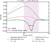 |
Fig. C.1. Illustration of the procedure used to measure the line parameters for a run with L = 0.6L*. Stot is the total spectrum in gray, SBB is the seed blackbody continuum in dashed black, Stot − SBB is the residual spectrum in red, and Cpoly is the sixth-order polynomial fit of the residual continuum spectrum, excluding the interval around the CRSF (pink shaded region). We measured the line width from the isolated absorption feature (Stot − SBB − Cpoly); green curve) as the FWHM (blue segment). Likewise, we estimated the centroid energy as the flux-weighted average energy within the region around the minimum where the absorption depth is larger than 90% of the maximum depth (red segment). |
We note that the choice of the excluded energy range in the polynomial fit can influence the final measurement; therefore, care must be taken in modeling the continuum to ensure stability. We varied the upper and lower limits of the exclusion zone by 10% to test the sensitivity of our inferences; the derived width and centroid energy change by less than 3%. We therefore consider the measurements robust, although a more sophisticated approach would further strengthen their validity.
All Tables
All Figures
|
Fig. 1. Illustration of the MC code’s geometry, coordinates, and calculation of the line-of-sight optical depth. A photon packet located at r0 is moving in direction |
| In the text | |
|
Fig. 2. Representative emergent spectrum for an XRP with a fiducial luminosity L = 0.6L*. The solid black line represents the seed blackbody spectrum with temperature kBT = 5.9 keV. The solid red line shows the total normalized emergent spectrum. The dashed blue and green lines correspond to the angle-selected spectra observed at polar angles in the ranges (0, π/2) and (π/2, π), respectively. The vertical dashed gray line indicates the cyclotron energy at Ec = 25.55 keV. The spectrum features a redshifted, but prominent CRSF around E ∼ 20 keV followed by a bump. The angle-selected spectra are scaled relative to their contribution to the total photon flux. |
| In the text | |
|
Fig. 3. Angle-resolved spectra for a typical XRP source with luminosity L = 0.6L*. The solid black line corresponds to the angle-averaged spectrum in the range (0, π/2). The dashed colored lines show spectra extracted in five angular bins within this range. Each spectrum has been normalized to its angular flux contribution. The vertical gray line marks the local cyclotron energy. With increasing cos θ, the CRSF centroid energy shifts to lower values and the blue wing becomes more pronounced. |
| In the text | |
|
Fig. 4. Angle-averaged emergent spectra for luminosities spanning the range L/L* ∈ (0, 1). The color gradient from dark blue to yellow corresponds to increasing luminosity. The inset highlights the spectral region around the CRSF. The vertical gray dashed line denotes the local cyclotron energy. The positive correlation between L and the CRSF energy ECRSF is evident. |
| In the text | |
|
Fig. 5. Dependence of the CRSF centroid energy ECRSF (panel a) and width σCRSF (panel b) on luminosity and viewing angle θ (measured with respect to the magnetic axis). Results are shown for five angular bins spanning the range θ ∈ (0, π/2), with Ec = 25.55 keV. Solid black lines denote quantities extracted from angle-averaged spectra. Both ECRSF and σCRSF exhibit a positive correlation with luminosity for all viewing angles. At a fixed luminosity, ECRSF (σCRSF) decreases (increases) toward smaller viewing angles, indicating substantial variability over the pulse cycle. |
| In the text | |
|
Fig. 6. Comparison of observed cyclotron line variability in GX 304-1 with our model. Panel a (b) shows the CRSF centroid energy (width). Red and black circles represent the observed ECRSF and σCRSF values of GX 304-1, obtained using the CYCLABS model (Lorentzian profile) and the GABS model (Gaussian profile), respectively, to fit the line feature (Mushtukov et al. 2015b). Green, blue, and purple lines correspond to the results derived from our MC simulations for three different viewing angle intervals. The model predictions, for specific viewing angles, agree sufficiently well with the data over an order of magnitude in luminosity. |
| In the text | |
|
Fig. A.1. Comparison of angle-averaged spectra with different boundary conditions for a typical source with luminosity L = 0.6L* and Ec = 25.55 keV (vertical gray dashed line). The solid black line represents the seed blackbody spectrum with kBT = 5.9 keV. The solid red (blue) line shows the emergent spectrum for the reflection (thermalization) case. The line wings exhibit differences; the red (blue) wing dominates in the thermalization (reflection) scheme. The centroid energy of the CRSF appears to be independent of the boundary condition. |
| In the text | |
|
Fig. A.2. Same as Fig. 4, but for the thermalization scheme. The luminosity dependence of the CRSF properties is the same. |
| In the text | |
|
Fig. A.3. Same as Fig. 5, but including the results obtained using the thermalization scheme in triangles connected with dashed lines. While the energy of the cyclotron feature is independent of the boundary scheme, the line width shows deviations at high luminosities. We expect this, as the redistribution of photons into the line wings alters the CRSF shape, affecting its width. |
| In the text | |
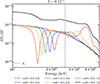 |
Fig. B.1. Same as Fig. 3, but for luminosity L = 0.1L*. |
| In the text | |
|
Fig. C.1. Illustration of the procedure used to measure the line parameters for a run with L = 0.6L*. Stot is the total spectrum in gray, SBB is the seed blackbody continuum in dashed black, Stot − SBB is the residual spectrum in red, and Cpoly is the sixth-order polynomial fit of the residual continuum spectrum, excluding the interval around the CRSF (pink shaded region). We measured the line width from the isolated absorption feature (Stot − SBB − Cpoly); green curve) as the FWHM (blue segment). Likewise, we estimated the centroid energy as the flux-weighted average energy within the region around the minimum where the absorption depth is larger than 90% of the maximum depth (red segment). |
| In the text | |
Current usage metrics show cumulative count of Article Views (full-text article views including HTML views, PDF and ePub downloads, according to the available data) and Abstracts Views on Vision4Press platform.
Data correspond to usage on the plateform after 2015. The current usage metrics is available 48-96 hours after online publication and is updated daily on week days.
Initial download of the metrics may take a while.