| Issue |
A&A
Volume 709, May 2026
|
|
|---|---|---|
| Article Number | L8 | |
| Number of page(s) | 9 | |
| Section | Letters to the Editor | |
| DOI | https://doi.org/10.1051/0004-6361/202659089 | |
| Published online | 06 May 2026 | |
Letter to the Editor
A break in planet occurrence near the pebble isolation mass should be observable by the Roman microlensing survey
1
Center for Star and Planet Formation, Globe Institute, Øster Voldgade 5, 1350 Copenhagen, Denmark
2
Space Telescope Science Institute, 3700 San Martin Drive, Baltimore, MD 21218, USA
★ Corresponding authors: This email address is being protected from spambots. You need JavaScript enabled to view it.
; This email address is being protected from spambots. You need JavaScript enabled to view it.
Received:
22
January
2026
Accepted:
30
March
2026
Abstract
Microlensing detections are uniquely well suited to probing the population of planets outside the water ice line, down to planetary masses comparable to the Earth’s. We performed 1D pebble-accretion population synthesis simulations to explore a sample of ice-line planets around stars with masses and metallicities similar to the target population of the Galactic Bulge Time-Domain Survey of the Nancy Grace Roman Space Telescope. We find that the planet distribution in the microlensing sensitivity space deviates from a log-uniform distribution in mass and orbital radius. When planetary core growth comes to a halt as planets reach the pebble isolation mass, Miso, the combined effects of planetary migration and runaway gas accretion create an occurrence break. Our simulations highlight that, between 1 and 50 AU, the fraction of stars that host isolation-mass planets (1–5 Miso) is lower by a factor of 20 compared to less massive planets (0.2–1 Miso). If this break in planetary occurrence rates around the pebble isolation mass is detected in future lensing surveys, it would further validate the core accretion paradigm for giant planet formation.
Key words: planets and satellites: detection / planets and satellites: formation / planets and satellites: general
© The Authors 2026
 Open Access article, published by EDP Sciences, under the terms of the Creative Commons Attribution License (https://creativecommons.org/licenses/by/4.0), which permits unrestricted use, distribution, and reproduction in any medium, provided the original work is properly cited.
This article is published in open access under the Subscribe to Open model. This email address is being protected from spambots. You need JavaScript enabled to view it. to support open access publication.
1. Introduction
Microlensing surveys are unique in their ability to detect sub-Earth-mass planets beyond the water ice line (Zhu & Dong 2021). The upcoming Galactic Bulge Time-Domain Survey by the Nancy Grace Roman Space Telescope (Roman) will be sensitive to 0.02 M⊕ planets at orbital distances of 4 AU, using the microlensing detection method, and is expected to yield around a thousand new lensing exoplanets (Penny et al. 2019). The microlensing detection technique is based on the detection of a magnification event (Gaudi 2012). This increase, or decrease, in the light curve of a background source star, typically at a distance of ≈8 kpc in the galactic bulge, is due to the gravitational perturbation of a foreground lens star, typically at a distance of ≈4 kpc. The presence of a planet around the lens star then creates small planetary caustics that induce variations in the single lens magnification event (Paczynski 1986). The typical host stars of lensing planets are M dwarfs, due to their higher occurrence in the galactic disc compared to solar-like stars (Chabrier 2005).
Previous work has argued that planet formation is efficient around M dwarf stars inside of the water ice line in the pebble accretion framework (Liu et al. 2020; Mulders et al. 2021; Chachan & Lee 2023). The exoplanet population synthesis model of Pan et al. (2025) finds that the super-Earth (SE) occurrence rate peaks around early M dwarfs (≈0.5 M⊙) and decreases towards late M dwarfs (0.1 − 0.2 M⊙) and solar-type stars (0.6 − 1 M⊙). In contrast, the occurrence rate of warm and cold giants monotonically increases with stellar mass. These theoretical findings appear to be consistent with observed links between occurrence rates and stellar masses (Mulders et al. 2015a; Hsu et al. 2020; Sabotta et al. 2021; Gillis et al. 2026). Building on these works, we expanded our previous exoplanet synthesis model (Danti et al. 2025) to investigate planet formation in the sensitivity domain of lensing surveys, around the ice line of a galactic stellar population.
2. Model
To perform the population synthesis simulations, we used a 1D pebble accretion model (Danti et al. 2025), with adjustment to account for stellar mass dependences (Appendix A). The planetary embryo’s seeds, taken from the top of the streaming instability distribution (Liu et al. 2020), grow by accreting pebbles (Ormel & Klahr 2010; Lambrechts & Johansen 2012) that are both drift- and fragmentation-limited in size (Brauer et al. 2008). The planetary embryos migrate through the disc in the type I migration regime (Paardekooper et al. 2010). Once the protoplanets reach isolation mass, they stop accreting solids (Lambrechts et al. 2014; see also Appendix A.3.1). Subsequently, the planets switch to type II migration (Kanagawa et al. 2018) and start accreting gas. The gas accretion phase is characterised by an initial slow Kelvin-Helmholtz contraction (Ikoma et al. 2000), followed by runaway gas accretion (Tanigawa & Tanaka 2016) that is limited by the accretion rate through the gap, which equals the gas accretion rate onto the central star (Lubow & D’Angelo 2006). The total amount of material available for solid accretion is given by a flux of pebbles set in the outer disc as a fraction, Z (which corresponds to the stellar dust-to-gas ratio), of the gas accretion rate onto the central star (Johansen et al. 2019). If multiple embryos are present (see Appendix B.3), the pebble flux is reduced by mutual pebble filtering (Guillot et al. 2014).
We used a disc model with a prescribed gas accretion rate, following Liu et al. (2020), and a temperature profile that can be entirely irradiated (Ida et al. 2016) or include moderate accretion heating (ϵel = 10−2; see Appendix A in Danti et al. 2025). The disc viscosity (αν) was fixed to 10−2 (Appelgren et al. 2023), while the turbulent stirring and fragmentation parameters were αz = αfrag = 10−4, representing a low-turbulence midplane as supported by recent observations of dust scale heights (Pinte et al. 2016) and fragmentation-limited particle sizes (Jiang et al. 2024). The inner edge of the disc was set to be the inner magnetospheric cavity (Liu et al. 2017).
3. Results
3.1. Dependence of the synthetic exoplanet population on the disc mass budget for typical lensing stars
An important uncertainty in our model is the poorly known scaling relation between stellar mass and the gas accretion rate onto the star,
 (1)
(1)
Here ṀH16 is the Hartmann et al. (2016) gas accretion rate observational fit anchored at M★ = 0.7 M⊙ (their Eq. (12)). The linear scaling (β = 1) and quadratic scaling (β = 2) represent, respectively, the weakest and steepest M★ dependences that encompass the observational spread (Alcalá et al. 2014; Manara et al. 2012; Venuti et al. 2014). We also explore a steeper-than-linear relation based on the observation of a large sample of sources in the Orion Nebula Cluster (Manara et al. 2012) in Appendix A.2. We simulated a set of 2000 single planets around a typical lensing star, M★ ≈ 0.2 M⊙ (Bochanski et al. 2010; Henry & Jao 2024), to explore the effects of the different gas accretion rate scalings with stellar mass, assuming either the β = 1 or β = 2 limit case (Eq. (1)).
For these synthetic populations, the stellar metallicities were sampled from Gaussian distributions that peaked at μ[Fe/H] = −0.02 with spread σ[Fe/H] = 0.22, following spectroscopic surveys of solar neighbour stars (Santos et al. 2005; Emsenhuber et al. 2021). The initial dust-to-gas ratio of the disc, Z, was then tied to the stellar metallicity through Z = 10[Fe/H]fdtg, ⊙, with the solar dust-to-gas ratio (fdtg, ⊙) set to 0.0149 (Lodders 2003); we assumed that the stellar metallicity distribution is independent of the stellar mass (Santos et al. 2003). The initial positions of the embryos were randomly drawn from a log-uniform distribution between 0.1 and 30 AU. Finally, the initial disc lifetime was randomly sampled from a normal distribution with a mean lifetime of μτ = 5 Myr and with a spread of στ = 0.5 Myr. The resulting synthetic populations are shown in Fig. 1, for a linear gas accretion scaling (top panel) and a quadratic one (bottom panel). The coloured boxes define the different types of planets, whose definitions can be found in Table B.1.
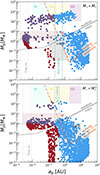 |
Fig. 1. Mass and semi-major axis of the synthetic populations of planets around 0.2 M⊙ stars, with our fiducial mass budget (Eq. (1) with β = 1; top) and a lower mass budget (Eq. (1) with β = 2; bottom). The colours represent icy embryos with initial and final positions outside the ice line (blue), mixed embryos that start outside and migrate to inside the ice line (purple), and rocky embryos with initial and final positions inside the ice line (red). The pebble isolation mass at the initial and final simulation time is marked by the dashed and solid grey line, respectively. The lensing sensitivity region, assuming the lens star is in the disc (4 kpc) and the source star is in the bulge (8 kpc), is marked with the dashed orange lines. The quadratic scaling of the accretion rate with stellar mass (bottom) hinders the formation of planets outside the ice line, as well as gas giants. |
The linear scaling of the gas accretion rate yields a population comprising ≈24% super-Earths and ≈10% gas giants, which is roughly consistent with the lower limit of the super-Earth occurrence rate,  , and the upper limit of the giant planet occurrence rate,
  , around M dwarfs (Sabotta et al. 2021). In contrast, the quadratic scaling with the accretion rate significantly hinders the growth of embryos, especially outside the ice line, resulting in discrepant occurrence fractions with respect to the observed exoplanet census.
For completeness, we also show in Appendix A.2 that the observationally motivated steeper-than-linear relation by Manara et al. (2012) similarly leads to small disc mass budgets in our model that under-predict the occurrence rate of super-Earths and gas giants. Given this, and the known large observational spread and uncertainties on stellar ages (Hartmann et al. 2016), we chose for simplicity a linear β = 1 scaling.
3.2. Planetary yields for a stellar lensing population
We now present our synthetic planet population drawn from N★ = 5000 stars sampling the initial mass function (IMF) distribution of Chabrier (2005), with stellar masses ranging from 0.01 to 5 M⊙, and assuming each star hosts a single planet. We calibrated the key parameters of the synthesis model such that we reproduced the observed super-Earth occurrence around FGK stars, P(SE) ≈ 30 − 50% (Zhu et al. 2018). The nominal model yields an occurrence of P(SE) ≈ 35% when assuming (i) a linear scaling of the gas accretion rate (Eq. (1); see Fig. 1, top panel), (ii) a particle fragmentation velocity of 10 m/s outside the ice line and 1 m/s inside the ice line, (iii) a moderate accretion-heated disc (see Appendix B.1 for the model calibration details and description). The left panel of Fig. 2 shows a break in occurrence above the pebble isolation mass (blue curves). This is a direct consequence of the combined effects of planet migration and runaway gas accretion, because planets that do make it beyond the isolation mass either migrate all the way to the inner disc or tend to grow into more massive gas giants. Therefore, the region above the pebble isolation around the ice line (≈1 AU) is depleted in planets.
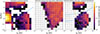 |
Fig. 2. Left panel: Synthetic exoplanet population, colour-coded by the number of planets per bin within the logarithmic semi-major axis and planet mass space, according to the nominal model for a sample of Nstar = 5000 stars with different masses (Sect. 3.2). For reference, we show the pebble isolation mass as a function of orbital radius, for a 0.2 M⊙ star, at the initial (dashed blue) and final simulation time (solid blue). Central panel: Total number of detected lensing planets per bin, assuming an underlying log-uniform distribution of 5000 planets in terms of semi-major axis and mass, with the lensing detection efficiency specified in Sect. 3.2. Annotated in each bin is the number of planets detected per bin, with the underlying number of planets in that bin in parentheses. The solid orange line shows the three-planet detection line for the Roman Space Telescope (Penny et al. 2019). Right panel: Total number of detected lensing planets per bin, using the synthetic population shown in the left panel. There is a dearth of planets with masses near the pebble isolation mass at the approximate location of the water ice line in the high-sensitivity region of lensing surveys. |
To provide a planetary yield from our synthetic population of planets, we first needed to estimate the detection sensitivity of a microlensing survey. The perturbation of the observed light curve due to the presence of a planet is strongest if the planet lies near the Einstein radius (at a projected separation s = ap/RE = 1, where ap is the planet’s semi-major axis and RE is the Einstein radius), with a decreasing efficiency at smaller (s < 1) and larger (s > 1) separations, and an increasing efficiency for larger planet-to-host star mass ratios (q = Mp/M★). In the case of a high-magnification event, this almost always results in a triangle-shaped detection efficiency in (q, s) space that, following Gould et al. (2010), can be parametrised as
 (2)
(2)
where η± are the left and right slopes of the triangle and qmin is the minimal detectable planetary mass ratio, corresponding to the bottom tip of the triangle, as illustrated in orange in Fig. 1. In our model we assumed 100% detection efficiency inside this triangle and 0% outside, which is roughly consistent with the detection efficiency triangles of high-magnification events (Gould et al. 2010) but slightly overestimates the detection efficiency in the tail of low-magnification events (Gould et al. 2010; Suzuki et al. 2016; see also Appendix C for the lensing sensitivity triangle description).
To model our lensing detection efficiency, we chose parameters that are broadly consistent with the Roman detection efficiency characterised in Penny et al. (2019). We parametrised the sensitivity triangle in the (q, s) space through Eq. (2), with qmin = 10−7, and two different slopes for the left and right side, η− = 0.25 and η+ = 0.85 (see the left panel of Fig. C.1). High-magnification events have a sensitivity that is nearly symmetrical in log s, implying η− = η+ (Gould et al. 2010; Choi et al. 2012), while more modest magnification events show higher sensitivities for planets with s > 1 and lower sensitivities for planets with s < 1 (Suzuki et al. 2016). This is because planets outside the Einstein ring (s > 1) cause perturbations in the higher-magnification major image created by the lens star, while planets inside the Einstein ring perturb the already lower-magnification minor image.
The central panel of Fig. 2 shows the total number of detected planets, assuming one planet per star and an underlying log-uniform distribution of planets in terms of semi-major axis and mass. This was obtained by multiplying the number of planets per mass-position bin by the detection efficiency in that specific bin. This figure shows that our simplified parametrisation qualitatively reproduces the reported detection efficiency of the Roman Space Telescope, assuming the same log-uniform planet distribution (Fig. 9 of Penny et al. 2019). This is also reflected in the decline of the detection efficiency (dark violet bins in the central panel of Fig. 2) that follows the so-called three-planet detection line predicted for Roman (light blue curve in Fig. 9 in Penny et al. 2019).
A planet distribution that is log-uniform in position and mass is not supported by our synthetic population (left panel of Fig. 2). Moreover, several observational studies have already shown, for example, a decreasing occurrence rate of gas giants at large orbital distances (Fulton et al. 2021) and gaps in the occurrence of inner disc planets with approximately 2 Earth radii (Fulton et al. 2017). Assuming our synthetic population as the underlying distribution (left panel Fig. 2), the right panel of Fig. 2 shows the expected planet yield in a Roman-like microlensing survey. Firstly, we note the presence of a population of detectable ice worlds, planets with masses between 1 and 10 M⊕ outside the water ice line, that have not yet been observed (Bitsch et al. 2015). Importantly, we recover in observational space the reduction in the number of detected planets above the pebble isolation mass, in the range [1 − 5] Miso, by a factor of 20 with respect to lower-mass planets in the range [0.2 − 1] Miso, for semi-major axes between 1 and 50 AU, and an increase in giant planet occurrence rates. We therefore argue that a lensing survey, such as the Galactic Bulge Time-Domain Survey of the Roman Space Telescope, should be able to detect this occurrence break. If correct, this would reduce the overall lensing yield of the Roman survey near this isolation break, compared to an assumed log-uniform mass and radius occurrence. At the same time, it would support the core accretion paradigm for gas giant formation as a two-step process consisting of the formation of solid migrating cores followed by a rapid epoch of gas accretion. If the break is not observed, then further studies on the gas accretion mechanisms that shape giant planet formation would need to be conducted.
4. Future work
A drop in the occurrence rate of planets above a critical core mass is a robust feature of population synthesis models, in both planetesimal-based (Ida & Lin 2004; Emsenhuber et al. 2021, 2025) and pebble-based (Bitsch et al. 2018; Liu et al. 2019) frameworks, even when using magnetohydrodynamic wind-driven, low-viscosity discs (Weder & Mordasini 2026). Observationally, some studies hint at the presence of such a depletion feature (Mayor et al. 2011; Bertaux & Ivanova 2022; Zang et al. 2025), while previous ground-based lensing surveys did not (Suzuki et al. 2018; Bennett et al. 2021). However, in a recent lensing study, Zang et al. (2025) show that there may be an occurrence break outside the water ice line. Clearly, a future larger lensing sample, such as the one to be provided by Roman, will be key to confirming or ruling out its existence.
Several aspects of this study should be explored in more detail to determine the robustness of our findings. Importantly, our results are sensitive to the disc model choice (see Sect. 3.1), which should be further explored, especially in the context of sub-solar stars (Arturo Rodriguez & Martin 2025). We used conventional migration prescriptions, but recent works highlight potential outward migration regimes for planets in the Earth-mass regime (Liu et al. 2015; Nielsen & Johansen 2025) and more massive gas giants (Sanchez et al. 2026). Moreover, our nominal model does not directly address planetary multiplicity, which is important for occurrence rate calculations. Although the role of mutual pebble filtering is minor (Appendix B.3), N-body studies show that the collisional growth of embryos can drive growth beyond the pebble isolation mass (Lambrechts et al. 2019; Sanchez et al. 2025). Ideally, these explorations would be conducted in a full population synthesis context (Burn et al. 2021; Pan et al. 2025; Chen et al. 2025) to further test key model assumptions and report theory-motivated planet yields for future lensing surveys.
Acknowledgments
We thank the anonymous referee for the helpful comments that improved the quality of this manuscript. C.D. thanks Lizxandra Flores-Rivera, Vera Sparrman and Adrien Houge for helpful discussion and Allison Youngblood for hosting the visit at NASA Goddard Space Flight Center. M.L. acknowledges the ERC starting grant 101041466 EXODOSS.
References
- Alcalá, J. M., Natta, A., Manara, C. F., et al. 2014, A&A, 561, A2 [NASA ADS] [CrossRef] [EDP Sciences] [Google Scholar]
- Appelgren, J., Lambrechts, M., & van der Marel, N. 2023, A&A, 673, A139 [NASA ADS] [CrossRef] [EDP Sciences] [Google Scholar]
- Armitage, P. J. 2010, Astrophysics of Planet Formation (Cambridge, UK: Cambridge University Press) [Google Scholar]
- Arturo Rodriguez, D. A., & Martin, R. G. 2025, MNRAS, 544, 3729 [Google Scholar]
- Batista, V., Dong, S., Gould, A., et al. 2009, A&A, 508, 467 [NASA ADS] [CrossRef] [EDP Sciences] [Google Scholar]
- Bennett, D. P., Ranc, C., & Fernandes, R. B. 2021, AJ, 162, 243 [NASA ADS] [CrossRef] [Google Scholar]
- Bertaux, J.-L., & Ivanova, A. 2022, MNRAS, 512, 5552 [NASA ADS] [CrossRef] [Google Scholar]
- Bitsch, B., Lambrechts, M., & Johansen, A. 2015, A&A, 582, A112 [NASA ADS] [CrossRef] [EDP Sciences] [Google Scholar]
- Bitsch, B., Morbidelli, A., Johansen, A., et al. 2018, A&A, 612, A30 [NASA ADS] [CrossRef] [EDP Sciences] [Google Scholar]
- Bochanski, J. J., Hawley, S. L., Covey, K. R., et al. 2010, AJ, 139, 2679 [NASA ADS] [CrossRef] [Google Scholar]
- Brauer, F., Dullemond, C. P., & Henning, T. 2008, A&A, 480, 859 [NASA ADS] [CrossRef] [EDP Sciences] [Google Scholar]
- Burn, R., Schlecker, M., Mordasini, C., et al. 2021, A&A, 656, A72 [NASA ADS] [CrossRef] [EDP Sciences] [Google Scholar]
- Chabrier, G. 2005, Astrophys. Space Sci. Lib., 327, 41 [NASA ADS] [CrossRef] [Google Scholar]
- Chachan, Y., & Lee, E. J. 2023, ApJ, 952, L20 [NASA ADS] [CrossRef] [Google Scholar]
- Chen, D.-C., Mordasini, C., Emsenhuber, A., et al. 2025, A&A, 701, A94 [NASA ADS] [CrossRef] [EDP Sciences] [Google Scholar]
- Choi, J.-Y., Shin, I.-G., Park, S.-Y., et al. 2012, ApJ, 751, 41 [Google Scholar]
- Danti, C., Lambrechts, M., & Lorek, S. 2025, A&A, 700, A132 [NASA ADS] [CrossRef] [EDP Sciences] [Google Scholar]
- Demircan, O., & Kahraman, G. 1991, Ap&SS, 181, 313 [Google Scholar]
- Emsenhuber, A., Mordasini, C., Burn, R., et al. 2021, A&A, 656, A69 [NASA ADS] [CrossRef] [EDP Sciences] [Google Scholar]
- Emsenhuber, A., Mordasini, C., Mayor, M., et al. 2025, A&A, 701, A64 [NASA ADS] [CrossRef] [EDP Sciences] [Google Scholar]
- Frank, J., King, A., & Raine, D. J. 2002, Accretion Power in Astrophysics: Third Edition (Cambridge, UK: Cambridge University Press) [Google Scholar]
- Fulton, B. J., Petigura, E. A., Howard, A. W., et al. 2017, AJ, 154, 109 [Google Scholar]
- Fulton, B. J., Rosenthal, L. J., Hirsch, L. A., et al. 2021, ApJS, 255, 14 [NASA ADS] [CrossRef] [Google Scholar]
- Gaudi, B. S. 2012, ARA&A, 50, 411 [Google Scholar]
- Gillis, E., Cloutier, R., & Pass, E. 2026, ArXiv e-prints [arXiv:2602.23364] [Google Scholar]
- Goldreich, P., & Tremaine, S. 1980, ApJ, 241, 425 [Google Scholar]
- Gould, A., Dong, S., Gaudi, B. S., et al. 2010, ApJ, 720, 1073 [NASA ADS] [CrossRef] [Google Scholar]
- Guillot, T., Ida, S., & Ormel, C. W. 2014, A&A, 572, A72 [NASA ADS] [CrossRef] [EDP Sciences] [Google Scholar]
- Hartmann, L., Herczeg, G., & Calvet, N. 2016, ARA&A, 54, 135 [Google Scholar]
- Henry, T. J., & Jao, W.-C. 2024, ARA&A, 62, 593 [Google Scholar]
- Hsu, D. C., Ford, E. B., & Terrien, R. 2020, MNRAS, 498, 2249 [Google Scholar]
- Ida, S., & Lin, D. N. C. 2004, ApJ, 604, 388 [Google Scholar]
- Ida, S., Guillot, T., & Morbidelli, A. 2016, A&A, 591, A72 [NASA ADS] [CrossRef] [EDP Sciences] [Google Scholar]
- Ikoma, M., Nakazawa, K., & Emori, H. 2000, ApJ, 537, 1013 [NASA ADS] [CrossRef] [Google Scholar]
- Jiang, H., Macías, E., Guerra-Alvarado, O. M., & Carrasco-González, C. 2024, A&A, 682, A32 [NASA ADS] [CrossRef] [EDP Sciences] [Google Scholar]
- Johansen, A., & Lambrechts, M. 2017, Ann. Rev. Earth Planet. Sci., 45, 359 [Google Scholar]
- Johansen, A., Ida, S., & Brasser, R. 2019, A&A, 622, A202 [NASA ADS] [CrossRef] [EDP Sciences] [Google Scholar]
- Johns-Krull, C. M. 2007, ApJ, 664, 975 [Google Scholar]
- Kanagawa, K. D., Tanaka, H., & Szuszkiewicz, E. 2018, ApJ, 861, 140 [Google Scholar]
- Lambrechts, M., & Johansen, A. 2012, A&A, 544, A32 [NASA ADS] [CrossRef] [EDP Sciences] [Google Scholar]
- Lambrechts, M., Johansen, A., & Morbidelli, A. 2014, A&A, 572, A35 [NASA ADS] [CrossRef] [EDP Sciences] [Google Scholar]
- Lambrechts, M., Morbidelli, A., Jacobson, S. A., et al. 2019, A&A, 627, A83 [NASA ADS] [CrossRef] [EDP Sciences] [Google Scholar]
- Lin, D. N. C., & Papaloizou, J. 1986, ApJ, 309, 846 [Google Scholar]
- Liu, B., Zhang, X., Lin, D. N. C., & Aarseth, S. J. 2015, ApJ, 798, 62 [Google Scholar]
- Liu, B., Ormel, C. W., & Lin, D. N. C. 2017, A&A, 601, A15 [NASA ADS] [CrossRef] [EDP Sciences] [Google Scholar]
- Liu, B., Lambrechts, M., Johansen, A., & Liu, F. 2019, A&A, 632, A7 [NASA ADS] [CrossRef] [EDP Sciences] [Google Scholar]
- Liu, B., Lambrechts, M., Johansen, A., Pascucci, I., & Henning, T. 2020, A&A, 638, A88 [EDP Sciences] [Google Scholar]
- Lodders, K. 2003, ApJ, 591, 1220 [Google Scholar]
- Lubow, S. H., & D’Angelo, G. 2006, ApJ, 641, 526 [Google Scholar]
- Manara, C. F., Robberto, M., Da Rio, N., et al. 2012, ApJ, 755, 154 [NASA ADS] [CrossRef] [Google Scholar]
- Manara, C. F., Rosotti, G., Testi, L., et al. 2016, A&A, 591, L3 [NASA ADS] [CrossRef] [EDP Sciences] [Google Scholar]
- Manara, C. F., Testi, L., Herczeg, G. J., et al. 2017, A&A, 604, A127 [NASA ADS] [CrossRef] [EDP Sciences] [Google Scholar]
- Mayor, M., Marmier, M., Lovis, C., et al. 2011, A&A, submitted [arXiv:1109.2497] [Google Scholar]
- Mulders, G. D., Pascucci, I., & Apai, D. 2015a, ApJ, 814, 130 [NASA ADS] [CrossRef] [Google Scholar]
- Mulders, G. D., Pascucci, I., & Apai, D. 2015b, ApJ, 798, 112 [Google Scholar]
- Mulders, G. D., Drążkowska, J., Marel, N. v. d., Ciesla, F. J., & Pascucci, I. 2021, ApJ, 920, L1 [NASA ADS] [CrossRef] [Google Scholar]
- Nielsen, J., & Johansen, A. 2025, A&A, 702, A90 [NASA ADS] [CrossRef] [EDP Sciences] [Google Scholar]
- Ormel, C. W., & Klahr, H. H. 2010, A&A, 520, A43 [NASA ADS] [CrossRef] [EDP Sciences] [Google Scholar]
- Paardekooper, S. J., Baruteau, C., Crida, A., & Kley, W. 2010, MNRAS, 401, 1950 [NASA ADS] [CrossRef] [Google Scholar]
- Paczynski, B. 1986, ApJ, 304, 1 [NASA ADS] [CrossRef] [Google Scholar]
- Pan, M., Liu, B., Jiang, L., et al. 2025, ApJ, 985, 7 [Google Scholar]
- Penny, M. T., Gaudi, B. S., Kerins, E., et al. 2019, ApJS, 241, 3 [CrossRef] [Google Scholar]
- Pinte, C., Dent, W. R. F., Ménard, F., et al. 2016, ApJ, 816, 25 [Google Scholar]
- Robin, A. C., Reylé, C., Derrière, S., & Picaud, S. 2003, A&A, 409, 523 [NASA ADS] [CrossRef] [EDP Sciences] [Google Scholar]
- Sabotta, S., Schlecker, M., Chaturvedi, P., et al. 2021, A&A, 653, A114 [NASA ADS] [CrossRef] [EDP Sciences] [Google Scholar]
- Sanchez, M., Paardekooper, S., van der Marel, N., Benítez-Llambay, P., & Mulders, G. D. 2025, A&A, 703, A169 [NASA ADS] [CrossRef] [EDP Sciences] [Google Scholar]
- Sanchez, M., van der Marel, N., Lambrechts, M., Paardekooper, S., & Miguel, Y. 2026, A&A, 705, A120 [NASA ADS] [CrossRef] [EDP Sciences] [Google Scholar]
- Santos, N. C., Israelian, G., Mayor, M., Rebolo, R., & Udry, S. 2003, A&A, 398, 363 [NASA ADS] [CrossRef] [EDP Sciences] [Google Scholar]
- Santos, N. C., Israelian, G., Mayor, M., et al. 2005, A&A, 437, 1127 [NASA ADS] [CrossRef] [EDP Sciences] [Google Scholar]
- Suzuki, D., Bennett, D. P., Sumi, T., et al. 2016, ApJ, 833, 145 [Google Scholar]
- Suzuki, D., Bennett, D. P., Ida, S., et al. 2018, ApJ, 869, L34 [NASA ADS] [CrossRef] [Google Scholar]
- Tanigawa, T., & Tanaka, H. 2016, ApJ, 823, 48 [NASA ADS] [CrossRef] [Google Scholar]
- Terry, S. K., Bachelet, E., Zohrabi, F., et al. 2026, AJ, 171, 212 [Google Scholar]
- Tychoniec, Ł., Manara, C. F., Rosotti, G. P., et al. 2020, A&A, 640, A19 [NASA ADS] [CrossRef] [EDP Sciences] [Google Scholar]
- van der Marel, N., & Mulders, G. D. 2021, AJ, 162, 28 [NASA ADS] [CrossRef] [Google Scholar]
- Venuti, L., Bouvier, J., Flaccomio, E., et al. 2014, A&A, 570, A82 [NASA ADS] [CrossRef] [EDP Sciences] [Google Scholar]
- Venuti, L., Stelzer, B., Alcalá, J. M., et al. 2019, A&A, 632, A46 [NASA ADS] [CrossRef] [EDP Sciences] [Google Scholar]
- Ward, W. R. 1997, Icarus, 126, 261 [Google Scholar]
- Weder, J., & Mordasini, C. 2026, A&A, 706, A335 [NASA ADS] [CrossRef] [EDP Sciences] [Google Scholar]
- Zang, W., Jung, Y. K., Yee, J. C., et al. 2025, Science, 388, 400 [Google Scholar]
- Zhu, W., & Dong, S. 2021, ARA&A, 59, 291 [NASA ADS] [CrossRef] [Google Scholar]
- Zhu, W., Petrovich, C., Wu, Y., Dong, S., & Xie, J. 2018, ApJ, 860, 101 [Google Scholar]
Appendix A: Stellar mass dependences
A.1. Stellar luminosity
We modelled the stellar mass dependence of the luminosity as a simple power law,
 (A.1)
(A.1)
as it is shown that young (< 10 Myr) stars have luminosities that scale like  before settling on a cubic relationship (Liu et al. 2020).
A.2. Stellar accretion rate
There have been different attempts to observationally constrain the gas accretion rate as a function of stellar mass. A recent spectroscopic surveys, based on observations of different star clusters, report a steeper-than-linear Ṁ★−M★ relation, with a 1.6-2.0 slope and 1-2 dex spread (e.g. Alcalá et al. 2014; Manara et al. 2017, 2016; Venuti et al. 2014, 2019; Hartmann et al. 2016). The spread in the power law dependence is likely the result of disc evolutionary processes and the initial condition scaling with stellar mass. Manara et al. (2012) provided a fitting formula for the gas accretion rate as a function of time and stellar mass based on observations of sources in the Orion Nebula Cluster:
 (A.2)
(A.2)
with M★ central host mass that ranges between 0.05 M⊙ and 2 M⊙ and t disc age. They point out that given the huge uncertainty on the disc age, this fit is invalid for t < 0.3 Myr.
Figure A.1 shows the same initial seed population around a 0.2 M⊙ star of Fig. 1 using the gas accretion scaling of Eq. A.2. This steeper-than-linear relation leads to a lower occurrence of both gas giants and super-Earths, though not as much as the quadratic relation (bottom panel of Fig. 1).
 |
Fig. A.1. Same as Fig. 1 but with the steeper-than-linear gas accretion rate of Eq. A.2 (Manara et al. 2012). |
A.3. Planetary embryos
We assumed that the planetary embryos were created through streaming instability within the first 105 years of the disc lifetime. We adopted the largest planetesimals formed by streaming instability as the planetary embryo, following Liu et al. (2020):
 (A.3)
(A.3)
Here f is a multiplicative factor that expresses how much the most massive planetesimals exceed the characteristic planetesimal mass of the measured size distribution, and γ is the dimensionless gravitational parameter,
 (A.4)
(A.4)
that measures the relative strength between the self-gravity of the disc and tidal shear. In our simulations, the discs are always non-self-gravitating (γ ≠ 1). Here we used f = 400, a = 0.5, b = 0, and C = 5 ⋅ 10−5 as in Liu et al. (2020).
A.3.1. Pebble isolation mass
Planetary embryos grow in the disc through pebble accretion (Ormel & Klahr 2010; Lambrechts & Johansen 2012) until they are massive enough to significantly perturb the gas in the disc. The threshold mass for which the gravitational perturbation due to the planet is able to create a pressure bump and halt the accretion of pebbles is called the pebble isolation mass. It can be expressed as
 (A.5)
(A.5)
where H/r is the gas disc aspect ratio (Johansen & Lambrechts 2017). In an irradiated disc (Ida et al. 2016), and for fragmentation-limited pebble sizes, the pebble isolation mass is almost independent of the stellar mass:
 (A.6)
(A.6)
Here we assumed the luminosity L★ scales with stellar mass as in Eq. A.1. This weak dependence no longer holds in the inner parts of protoplanetary discs, where time-dependent accretion heating can modify the gas scale height (see Appendix A in Danti et al. 2025). In this case, the pebble isolation mass is proportional to
 (A.7)
(A.7)
with θ = −11/20 in case of a linear scaling of the stellar accretion rate with stellar mass (Eq. 1, with β = 1) and θ = 23/20, for the limit case of a quadratic scaling (Eq. 1, with β = 2). Therefore, in the inner disc the pebble isolation mass is sensitive to the assumed accretion rate prescription (Liu et al. 2019), but this complication does not affect lensing planets located outside the ice line (Fig. 1).
A.3.2. Planet migration
The planetary embryos (Eq. A.3) grow through pebble accretion and migrate through the disc at the same time. As they are still embedded in the disc, the asymmetric torque due to Lindblad resonances and co-rotation leads to inwards type I migration (Goldreich & Tremaine 1980; Ward 1997). As they grow more massive, the embryos perturb the gas in the disc, creating a gap and reducing their migration rate, falling into the slower type II migration (Lin & Papaloizou 1986), that we modelled according to Kanagawa et al. (2018).
The inwards migration of the planet is halted at the inner edge of the disc, represented by the magnetospheric cavity as in Frank et al. (2002), Armitage (2010), and Liu et al. (2017):
 (A.8)
(A.8)
where B★ is the stellar magnetic field, R★ the stellar radius, M★ the stellar mass and ̇M★ the accretion rate on the central star (see Sect. 2). We set our nominal values to B★ = 1 kG, representative of a typical solar mass T-Tauri star (e.g. Johns-Krull 2007). To model the relation between star radius and mass, we adopted the empirical relation (Demircan & Kahraman 1991)
 (A.9)
(A.9)
Appendix B: Model calibration and variations
B.1. Fiducial model calibration
We calibrated our nominal model in order to roughly reproduce the occurrence rate of super-Earths around FGK stars, P(SE) ≈ 30 − 50% (Zhu et al. 2018). To find the best fit model, we simulated 5000 planets in a purely irradiated disc (left panel of Fig. B.1) and a moderately accretion-heated disc (right panel of Fig. B.1), using a linear gas accretion rate scaling (see Sect. 3.1 and Fig. 1). The initial positions of the planetary embryos were randomly drawn from a log-uniform distribution between 0.1 and 30 AU, and the initial masses were taken from the top of the streaming instability (Eq. A.3). The stellar masses were randomly sampled from the Chabrier (2005) IMF distribution, limited to the range 0.01 − 5 M⊙. The stellar metallicities were sampled from a Gaussian distribution that peaks at μ[Fe/H] = −0.02 with spread σ[Fe/H] = 0.22 (Emsenhuber et al. 2021). The initial dust-to-gas ratio of the disc, Z, was then calculated from the star metallicity as Z = 10[Fe/H]fdtg, ⊙, with fdtg, ⊙ = 0.0149 following Lodders (2003). The accreted pebbles are both fragmentation- and drift-limited in size (Brauer et al. 2008). The value of the fragmentation velocity changes from 10 m/s to 1 m/s when the pebbles cross the ice line, which is defined as the location in the disc where the temperature is T = 170 K. The disc viscosity is fixed at αν = 10−2 (Appelgren et al. 2023), while the turbulent stirring and fragmentation parameters are both fixed at αz = αfrag = 10−4, representing a low-turbulence midplane supported by recent dust scale heights observations (Pinte et al. 2016) and by observational estimates of fragmentation-limited particle sizes. We random sample disc lifetimes, τdisc, from a Gaussian distribution with mean μτ = 5 Myr and standard deviation στ = 0.5 Myr. This results in a solid disc mass distribution with median mass of Mdust, tot ≈ 500 M⊕ for a linear scaling of gas accretion rate with stellar mass (Eq. 1, β = 1) and Mdust, tot ≈ 240 M⊕ for super-linear scaling (Eq. A.2). We verified that this randomly sampled initial dust disc mass distribution is consistent with that inferred from observations of discs around young stars (Tychoniec et al. 2020) and population synthesis models of pebble disc evolution (Appelgren et al. 2023).
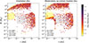 |
Fig. B.1. Left panel: Population synthesis of 5000 planets for an irradiated disc, with linear scaling of the gas accretion rate with stellar masse (Eq. 1, β = 1), randomly sampled Z, and disc lifetimes from Gaussian distributions (Appendix B.1), and M★ from the Chabrier (2005) IMF restricted to the range 0.01 − 5 M⊙. The colour-coding shows the disc lifetime. Right panel: Same as the left panel but for a moderately accretion-heated disc. The bottom left box shows the occurrence fraction of the different types of planets in both cases. We chose to use as a fiducial model the moderately accretion-heated disc (right panel) as the occurrence rate of super-Earths is broadly consistent with observations (Zhu et al. 2018). |
Figure B.1 shows the comparison between the population of planets for an irradiated disc (left) and for a moderately accretion-heated disc (right), colour-coded for disc lifetime. The occurrence rates of each type of planet in Table B.1 are listed in the bottom left corner. The moderately accretion-heated model provides a better fit to the observed super-Earth exoplanet population, therefore we chose this as the nominal disc model.
Planet type definitions.
B.2. Disc metallicity
To investigate how the initial disc metallicity affects the planets’ final semi-major axis and mass distribution, we performed a set of single planet simulations for a fixed M★ = 0.2 M⊙ star, using the nominal accretion-heated disc. The initial conditions of the simulations are the same as described in the model calibration of Sect. 2, with the exception of the fixed stellar mass and the fixed initial disc metallicity from Z = 0.010, 0.015, 0.020, 0.025, and 0.030. The three panels of Fig. B.2 show the final semi-major axes and masses of the planet populations for the three different gas accretion rates: linear dependence in the top panel (Eq. 1 with β = 1), steeper-than-linear for the central panel (Eq. A.2), and quadratic dependence for the bottom panel (Eq. 1 with β = 2). The colour-coding represents the fixed initial disc metallicity Z. Finally, the inset plots show the occurrence rates of super-Earths and giant planets (black and brown lines, respectively).
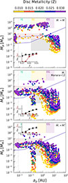 |
Fig. B.2. Semi-major axis and masses of a synthetic population of planets orbiting a 0.2 M⊙ star, colour-coded by initial disc metallicity. The three panels correspond to the three different gas accretion rates: Eq. 1 with β = 1 (top), Eq. A.2 (centre), and Eq. 1 with β = 2 (bottom). The dashed and solid purple lines represent the pebble isolation mass at the initial and final simulation time, respectively. The insets show the occurrence rate of super-Earths (black lines) and giant planets (brown lines) as a function of the initial disc metallicity. |
Simulations with higher disc metallicity show a clear increasing trend of giant planet occurrence, when assuming a linear gas accretion rate (top panel of Fig. B.2, brown line of the inset plot), as already supported by multiple theoretical (e.g. Pan et al. 2025) and observational studies (Mulders et al. 2015b; van der Marel & Mulders 2021). A steeper-than-linear gas accretion rate with stellar mass (central and bottom panels of Fig. B.2) leads to almost no gas giant formation as the mass budget and the pebble accretion efficiency are too low, regardless of the initial disc metallicity. The super-Earths occurrence rate shows a flat trend with increasing initial disc metallicity in case of the linear gas accretion rate (top panel of Fig. B.2, black line of the inset plot), while it increases for steeper-than-linear stellar mass dependences (central and bottom panel of Fig. B.2), with significant occurrence only in high metallicity discs with Z > 0.02. This is due to the fact that the solid mass budget is lower than in the linear case, therefore a higher disc metallicity provides the needed increase in mass for more efficient super-Earth formation. In the case of lower-mass planets (sub-Earths), a higher initial disc metallicity leads to slightly more massive planets.
B.3. Multiplicity: Four-planet population
We investigated the role of mutual filtering between embryos by running systems of four planetary embryos each, randomly sampled from a log-uniform distribution in semi-major axis between 0.1 and 30 AU, and using a fixed disc lifetime of 5 Myr. Figure B.3 shows example growth tracks of the planets in our four-planet system simulations, marked by a solid line when pebble filtering is included and by a dashed line when pebble filtering is not included. Each colour identifies a different randomly drawn system of four planets. The lensing sensitivity triangle is marked by the dashed orange lines.
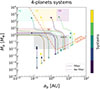 |
Fig. B.3. Growth tracks of five systems of four planets (in different colours). The solid (dashed) lines show the simulations where mutual pebble filtering is (is not) accounted for. |
We find that the occurrence rate of lensing planets is hardly affected by the multiplicity of the system. Mutual filtering is irrelevant in the lensing corner, at most leading to slightly lower masses in the inner disc (see the innermost teal planet in Fig. B.3).
Appendix C: The lensing sensitivity triangle
The microlensing sensitivity calculated through Eq. 2 results in a triangle-shaped detection efficiency in the (q, s) space, which has been observed to nicely reproduce most of the high magnification events (Gould et al. 2010). The tip of the sensitivity triangle, qmin, which depends on the specifics of the instrument and on the microlensing event, is parametrised as
 (C.1)
(C.1)
where ξ ≈ 1/50 is a parameter that depends on the quality of data, while Amax is the maximum magnification. Here, 1/Amax essentially probes how close the source comes to the central caustic of the system (Gould et al. 2010)
Parameterising the survey sensitivity with a triangle of 100% detection efficiency inside and 0% outside is a reasonable approximation for high-magnification events, which are nearly symmetrical in log s (Gould et al. 2010; Choi et al. 2012), but overestimates the detection efficiency in case of mid and low-magnification events, that show higher sensitivities outside the Einstein ring (s > 1) because the magnification is the result of the planetary perturbation of the major image which is brighter Suzuki et al. (2016). In case of a primary event with magnification A, the perturbation of the major image results in a magnification (A + 1)/2, while the perturbation of the minor image is (A − 1)/2, therefore, as A → 1, the only observable magnification events are the ones that perturb the major image (s > 1). The sensitivity for low magnification events also tends to be lower at exactly the Einstein separation, leading to a W-shaped rather than triangular-shaped detection efficiency (e.g. Suzuki et al. 2016). In principle, the planet detection efficiency is not only a function of (q, s) but also α, the angle of the source-lens trajectory relative to the planet-star axis, but the narrowness of the boundary region between 100% and 0% detection efficiency suggests it to be nearly independent of α (Batista et al. 2009; Gould et al. 2010), hence we do not parametrise it.
In order to estimate the number of detected planets from our underlying planet distribution, we mapped (Mp, ap) into the (q, s) space to check the detectability of the planet, making use of
 (C.2)
(C.2)
where ML is the lens (host) star mass and RE the Einstein radius:
 (C.3)
(C.3)
Here DL and DS are the lens and source star distances, whose nominal values, assuming they are a disc and bulge star respectively, are 4 and 8 kpc. The Einstein ring is defined as
 (C.4)
(C.4)
where DLS is the lens to source distance and c is the speed of light.
As we see from the above expressions, the (q, s)→(Mp, ap) mapping requires knowledge of the lens (host) star mass. When dealing with our synthetic population of planets, we know the star’s masses as we draw them from a given IMF distribution (for Fig. 2, based on the Chabrier 2005 IMF). Also, for real observed lensing exoplanets, the uncertainty on the stellar mass introduces an important uncertainty on the planet’s properties. Estimates of the host star mass are possible if the event is long enough to measure the effect of the annual microlensing parallax or if it is observed from two widely separated observers, which proves difficult for microlensing surveys, especially from the ground. High-resolution imaging provides an alternative method to estimate the host star’s mass by measuring the separation between source and host star and the host star’s colour and magnitude. The Roman Space Telescope will be able to make these measurements routinely for most of the events (Penny et al. 2019). It is indeed expected that Roman will be able to determine the lens star masses and distances with uncertainties of less than 20% for half of the events and over 40% for all of them (Terry et al. 2026).
The left panel of Fig. C.1 shows how we parametrised the lensing sensitivity in the (q, s) space throughout this paper, where we approximated a detectability of 100 % inside the sensitivity triangle and 0% outside. The parameters that define the triangle through Eq. 2 have values qmin = 10−7, η+ = 0.85 and η− = 0.25 to roughly match the Roman sensitivity. The central and right panels of Fig. C.1 show an example of the detectability of a sample of synthetic planets drawn from a log-uniform distribution in mass and semi-major axis (same as the central panel of Fig. 2), assuming two different underlying stellar IMFs. The central panel draws from the Robin et al. (2003) stellar IMF, while the right panel draws from the Chabrier (2005) IMF. The colour-coding represents the number of detected planets in each bin, which, in the underlying log-uniform synthetic planet distribution, are ≈ 50 × 103 planets per bin. For comparison, the coloured contours depict the Roman sensitivity detection lines from Penny et al. (2019), assuming one planet per star, with the 3-detection line marked in light blue. Given our 100% detectability inside and 0% outside the triangle, we tend to generally overestimate the detectability of planets, as shown from the comparison to the Roman sensitivity contours in the central and right panel of Fig. C.1. Nonetheless, the break of planet occurrence near the ice line (right panel of Fig. 2) would hold even with a more accurate sensitivity estimation, as it appears in a region where the sensitivity of microlensing from space is reasonably close to unity.
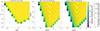 |
Fig. C.1. Left panel: Sensitivity in the (q, s) space for a log-uniform distribution of synthetic planets. Centre and right panels: Detected planets from a log-uniform distribution of synthetic planets in (Mp, ap), for two different star IMFs: the Robin et al. (2003) disc stars power law (centre) and the Chabrier (2005) IMF (right). The colour-coding indicates the total number of detected stars in each bin. The contours show the detection sensitivity lines of Roman from Penny et al. (2019), with the three-detection line in cyan, assuming one planet per star. |
The comparison between the central and right panel of Fig. C.1 also shows how the estimate of the mass of the lensing star affects our ability to detect a planet with a certain mass Mp orbiting at a certain distance ap. As the planetary caustics depend on the planet-to-star mass ratio, the same type of planet orbiting a different type of star might not be visible. The Chabrier (2005) stellar IMF from the right panel is peaked around 0.2 M⊙, while the central panel IMF (Robin et al. 2003) peaks around less massive stars. The lensing sensitivity in the right panel decreases more gradually for lower q and further away from the Einstein radius. This happens because for a fixed planet mass, Mp, orbiting at a fixed distance, ap, an increase in the mass of the host star, ML, implies a lower mass ratio, q, and a higher projected separation, s (Eq. 2), therefore effectively pushing the planet outside of the detection sensitivity triangle.
All Tables
All Figures
|
Fig. 1. Mass and semi-major axis of the synthetic populations of planets around 0.2 M⊙ stars, with our fiducial mass budget (Eq. (1) with β = 1; top) and a lower mass budget (Eq. (1) with β = 2; bottom). The colours represent icy embryos with initial and final positions outside the ice line (blue), mixed embryos that start outside and migrate to inside the ice line (purple), and rocky embryos with initial and final positions inside the ice line (red). The pebble isolation mass at the initial and final simulation time is marked by the dashed and solid grey line, respectively. The lensing sensitivity region, assuming the lens star is in the disc (4 kpc) and the source star is in the bulge (8 kpc), is marked with the dashed orange lines. The quadratic scaling of the accretion rate with stellar mass (bottom) hinders the formation of planets outside the ice line, as well as gas giants. |
| In the text | |
|
Fig. 2. Left panel: Synthetic exoplanet population, colour-coded by the number of planets per bin within the logarithmic semi-major axis and planet mass space, according to the nominal model for a sample of Nstar = 5000 stars with different masses (Sect. 3.2). For reference, we show the pebble isolation mass as a function of orbital radius, for a 0.2 M⊙ star, at the initial (dashed blue) and final simulation time (solid blue). Central panel: Total number of detected lensing planets per bin, assuming an underlying log-uniform distribution of 5000 planets in terms of semi-major axis and mass, with the lensing detection efficiency specified in Sect. 3.2. Annotated in each bin is the number of planets detected per bin, with the underlying number of planets in that bin in parentheses. The solid orange line shows the three-planet detection line for the Roman Space Telescope (Penny et al. 2019). Right panel: Total number of detected lensing planets per bin, using the synthetic population shown in the left panel. There is a dearth of planets with masses near the pebble isolation mass at the approximate location of the water ice line in the high-sensitivity region of lensing surveys. |
| In the text | |
|
Fig. A.1. Same as Fig. 1 but with the steeper-than-linear gas accretion rate of Eq. A.2 (Manara et al. 2012). |
| In the text | |
|
Fig. B.1. Left panel: Population synthesis of 5000 planets for an irradiated disc, with linear scaling of the gas accretion rate with stellar masse (Eq. 1, β = 1), randomly sampled Z, and disc lifetimes from Gaussian distributions (Appendix B.1), and M★ from the Chabrier (2005) IMF restricted to the range 0.01 − 5 M⊙. The colour-coding shows the disc lifetime. Right panel: Same as the left panel but for a moderately accretion-heated disc. The bottom left box shows the occurrence fraction of the different types of planets in both cases. We chose to use as a fiducial model the moderately accretion-heated disc (right panel) as the occurrence rate of super-Earths is broadly consistent with observations (Zhu et al. 2018). |
| In the text | |
|
Fig. B.2. Semi-major axis and masses of a synthetic population of planets orbiting a 0.2 M⊙ star, colour-coded by initial disc metallicity. The three panels correspond to the three different gas accretion rates: Eq. 1 with β = 1 (top), Eq. A.2 (centre), and Eq. 1 with β = 2 (bottom). The dashed and solid purple lines represent the pebble isolation mass at the initial and final simulation time, respectively. The insets show the occurrence rate of super-Earths (black lines) and giant planets (brown lines) as a function of the initial disc metallicity. |
| In the text | |
|
Fig. B.3. Growth tracks of five systems of four planets (in different colours). The solid (dashed) lines show the simulations where mutual pebble filtering is (is not) accounted for. |
| In the text | |
|
Fig. C.1. Left panel: Sensitivity in the (q, s) space for a log-uniform distribution of synthetic planets. Centre and right panels: Detected planets from a log-uniform distribution of synthetic planets in (Mp, ap), for two different star IMFs: the Robin et al. (2003) disc stars power law (centre) and the Chabrier (2005) IMF (right). The colour-coding indicates the total number of detected stars in each bin. The contours show the detection sensitivity lines of Roman from Penny et al. (2019), with the three-detection line in cyan, assuming one planet per star. |
| In the text | |
Current usage metrics show cumulative count of Article Views (full-text article views including HTML views, PDF and ePub downloads, according to the available data) and Abstracts Views on Vision4Press platform.
Data correspond to usage on the plateform after 2015. The current usage metrics is available 48-96 hours after online publication and is updated daily on week days.
Initial download of the metrics may take a while.