


| Issue |
A&A
Volume 709, May 2026
|
|
|---|---|---|
| Article Number | A233 | |
| Number of page(s) | 9 | |
| Section | Extragalactic astronomy | |
| DOI | https://doi.org/10.1051/0004-6361/202558642 | |
| Published online | 19 May 2026 | |
MUSE Analysis of Gas around Galaxies (MAGG)
VII. Emission line galaxies near strong blended Lyα absorption systems at z ≳ 3
1
Dipartimento di Fisica “G. Occhialini”, Università degli Studi di Milano-Bicocca, Piazza della Scienza 3, I-20126 Milano, Italy
2
INAF – Osservatorio Astronomico di Trieste, Via G. B. Tiepolo 11, I-34143 Trieste, Italy
3
INAF – Osservatorio Astronomico di Brera, Via Brera 28, I-21021 Milano, Italy
4
Aix Marseille Université, CNRS, CNES, LAM, Marseille, France
★ Corresponding author: This email address is being protected from spambots. You need JavaScript enabled to view it.
Received:
18
December
2025
Accepted:
9
April
2026
Abstract
We investigate the connection between strong, blended Lyα absorption systems (SBLAs) and ≈1000 Lyα-emitting galaxies (LAEs) at z ≳ 3 in 28 quasar fields from the MUSE Analysis of Gas around Galaxies (MAGG) survey. Selecting SBLAs as spectral regions with transmitted flux −0.05 < F < 0.25 over ≈ 138 km s−1 bins, we find a strong correlation with LAEs within a projected distance of R ≤ 300 kpc and line-of-sight velocity separation of |Δv| ≤ 300 km s−1. The association rate increases significantly with decreasing flux, a trend that persists also at smaller separations (R < 100 kpc). A two-dimensional cross-correlation analysis confirms significant clustering of LAEs around SBLAs, while no such clustering is seen for spectral regions with F > 0.25. The correlation appears to also depend on the width of the spectral window used to identify SBLAs, with a larger window yielding a stronger signal. Our analysis confirms that SBLAs serve as probes of the circumgalactic medium (CGM) at the interface between the Lyα forest and the optically thick Lyman limit systems. The significant dependence of the LAE-SBLA cross-correlation on the spectral binning used to select these absorbers motivates future tests of the current SBLA framework as a tracer of halos.
Key words: galaxies: halos / galaxies: high-redshift / intergalactic medium / quasars: absorption lines
© The Authors 2026
 Open Access article, published by EDP Sciences, under the terms of the Creative Commons Attribution License (https://creativecommons.org/licenses/by/4.0), which permits unrestricted use, distribution, and reproduction in any medium, provided the original work is properly cited.
This article is published in open access under the Subscribe to Open model. This email address is being protected from spambots. You need JavaScript enabled to view it. to support open access publication.
1. Introduction
The mapping of neutral hydrogen (H I) using absorption spectroscopy of bright background quasars has led to a rich taxonomy of absorption line systems (ALSs), including high column densities damped Lyα absorbers (DLAs; NHI ≥ 1020.3 cm−2, Wolfe et al. 2005); intermediate population of super Lyman limit systems (SLLSs also known as sub-DLAs; NHI ≥ 1019 cm−2, Péroux et al. 2002); optically thick Lyman limit systems (LLSs; NHI ≥ 1017.2 cm−2, Tytler 1982); and the optically thin Lyα forest (Lynds 1971). In addition to the empirical classification based on the observed column densities, the statistical properties of these various ALSs connect specific classes to identifiable cosmic structures. The DLAs are often associated with the densest portion of the circumgalactic medium (CGM), broadly defined as the gas that extends beyond the galaxy disks and is confined within a few virial radii, including the disk-halo interface and the outer H I disks of galaxies, especially at low redshifts (Wolfe et al. 2005; Fumagalli et al. 2011). The LLSs, with their partial ionization and inferred volume densities of 10−3−10−1 cm−3 (Fumagalli et al. 2016), are one of the best tracers of the z ≈ 3 CGM but can also probe dense regions of the intergalactic medium (IGM) at higher redshift (z ≳ 3.5), where the mean neutral fraction of the Universe becomes significant enough to form slabs of partially neutral gas even at modest overdensities (Fumagalli et al. 2013). Finally, the Lyα forest is the tracer of the gas filaments that make up the IGM (Rauch 1998).
However, nature does not make jumps, and the above scheme is bound to be incomplete or even inaccurate, especially at the transition points between classes. This is especially the case since the mapping between physical overdensities (i.e., volume densities compared to the mean cosmological density) and column density is not a tight one-to-one relation due to local fluctuations arising from gas clumpiness or variation in the ionization field (Rahmati et al. 2013). The nature of the transition region occupied by SLLSs and sub-DLAs has been actively debated (Khare et al. 2007). More recently, the transition between LLSs and the Lyα forest has been the subject of renewed attention. The gas at H I column densities of 1014−1016 cm−2 is highly relevant for its contribution to the mean opacity of the Universe (Prochaska et al. 2010). Moreover, due to the multiphase nature of the CGM, which extends over a very wide range of densities and thermal and ionization conditions (Tumlinson et al. 2017), the detailed contribution of halo gas in the transition region between LLSs and the Lyα forest is becoming a relevant question.
This transition region has been the focus of a series of articles on the so-called “strong, blended Lyα forest absorption systems” (SBLAs; Pieri et al. 2010, 2014; Pérez-Ràfols et al. 2023; Morrison et al. 2024). This class of absorbers is identified via low transmission pixels on a set velocity scale, which can arise whenever multiple strong Lyα lines are clustered in velocity. One of the approaches suggested to identify SBLAs is based on quasar spectra with a signal-to-noise ratio per pixel S/N > 3 over a 100-pixel boxcar from the Baryon Oscillation Spectroscopic Survey (BOSS). Absorbed pixels with transmitted flux F < 0.25, once rebinned by a factor of two in the Sloan Digital Sky Survey (SDSS) velocity scale of 138 km s−1, select the SBLAs. Specific transmission ranges further define subclasses of this population (e.g., −0.05 < F < 0.05 representing the FS0 class of the strongest systems; Pieri et al. 2014; Morrison et al. 2024). DLAs are masked and excluded from selection to avoid contamination. Due to their mixed nature, a combination of individual absorbers of different H I and metal content contributes to the SBLA population, which can, however, be studied with spectral stacking (Pieri et al. 2014). Modeling of the Lyman limit of the SBLA composite spectrum suggests column densities NHI < 1016 − 1016.5 cm−2 (Pieri et al. 2014). This limit can be refined further by considering the Lyman series lines, resulting in three different SBLAs samples with increasing column density as a function of decreasing transmitted flux thresholds, NHI ≈ 1015.11 cm−2, NHI ≈ 1015.64 cm−2, and NHI ≈ 1016.04 cm−2 (Morrison et al. 2024). Thus, SBLAs are mainly optically thin systems that represent a transition population between LLSs and the weaker Lyα forest.
The analysis of the metal content of SBLAs provides further insight into the physical origin of this population. The SBLAs are a heterogeneous class of metal absorbers composed of strong metal lines for ≈1/4 of their population, especially in a low-ionization phase (Morrison et al. 2024). Higher ionization gas appears to be more widespread within SBLAs. Detailed photoionization modeling of SBLA composite spectra, under the assumption of optically thin gas, reveals a multiphase medium composed of at least three distinct phases of density and temperature: a low-ionization phase with nH = 1 cm−3 and metallicity [X/H] = 0.8, an intermediate-ionization phase with nH = 10−3 cm−3 and metallicity [X/H]= − 0.8, and a high-ionization phase whose physical parameters are poorly constrained.
Additional insight into the astrophysical structures that give rise to SBLAs originates from a clustering analysis (Pérez-Ràfols et al. 2023; Morrison et al. 2024). The cross-correlation of SBLAs with the Lyα forest provides a bias of 2.329 ± 0.057, consistent with that of DLAs. Thus, SBLAs are likely to arise from dark-matter overdensities comparable to halos of masses ≈ 0.5−1 × 10¹² M⊙. This finding, together with evidence that SBLAs are a multiphase and enriched population, provides a strong link between this class of absorbers and the CGM of galaxies. Hence, SBLA and DLA systems probably trace different portions of the CGM of a similar population of galaxies (Pérez-Ràfols et al. 2023). This hypothesis can be verified explicitly by cross-correlating SBLAs with galaxy populations. By performing this experiment in quasar fields with surveys of Lyman break galaxies (LBGs), Pieri et al. (2014) found that SBLAs with F < 0.25 reside near an LBG on average 60 percent of the time. Therefore, SBLAs selected at F < 0.25 are ten times more likely to be associated with LBGs than spectral pixels with F > 0.75, and are five times more likely to be near LBGs than for a random distribution. Moreover, in a recent simulation work using TNG50, Muñoz Santos et al. (2025) show that SBLAs are highly efficient halo finders. In SDSS-like spectra, up to ≈80 percent of systems with low Lyα transmission (F < 0.05) reside within dark-matter halos and are associated with halos with masses of ≈1012 M⊙. By adopting a hierarchical approach, they refined the selection of SBLAs, with larger systems consuming smaller ones, and obtained a narrower halo mass distribution compared to the non-hierarchical framework. This is consistent with the observational constraints derived by clustering analysis, reinforcing the interpretation of SBLAs as robust tracers of the CGM around massive galaxies.
However, the statistics originating from the correlations of SBLAs and LBGs are significantly dependent on the completeness correction in the LBG surveys. Thanks to integral field spectrographs (IFSs) such as the Multi Unit Spectroscopic Explorer (MUSE) (Bacon et al. 2010) at the Very Large Telescope (VLT), dense and highly complete z ≳ 3 redshift surveys are available. This enables further testing of the hypothesis that SBLAs trace the CGM of fairly massive cosmic structures. In this paper, we rely on the “MUSE Analysis of Gas around Galaxies” (MAGG) survey to test the link between Lyα emitters (LAEs) and SBLAs in the redshift interval 2.5 < z < 4.5. MAGG is a moderate depth MUSE/IFS redshift survey of 28 quasar fields at z ≈ 3.5 − 4, for which high resolution and high S/N quasar spectroscopy are available (Lofthouse et al. 2020). At z > 3, the MAGG survey has already revealed tight correlations between LAEs and strong H I, C IV, and a fraction of Mg II absorption line systems (Lofthouse et al. 2023; Galbiati et al. 2023, 2024). However, the bulk of the ALSs arise not from the CGM of the LAEs, but from the large-scale gas filaments within which the galaxies are embedded. Moreover, MAGG uncovered a substantial dependence of the gas properties of LAEs on their galactic environment, with group galaxies embedded in more gas-rich regions (Lofthouse et al. 2023; Galbiati et al. 2023, 2024; see also Dutta et al. 2020, 2021).
With the complete and homogeneous sample of X-Shooter spectra for the 28 MAGG quasars (Galbiati et al. 2024) and a catalog of ≈1000 LAEs with well-characterized completeness (Galbiati et al. 2023), we directly investigate the link between SBLAs and moderate-mass Lyα-emitting galaxies. The purpose of this study is therefore to provide additional information on whether this class of absorbers arises from the CGM and which is the more likely population of parent halos. We structure this paper as follows. In Section 2, we present a brief overview of the available data. We describe the selection of SBLAs in the MAGG quasar spectra in Section 3. The results of the SBLA-LAE correlation are given in Section 4. A discussion of our findings and conclusions is provided in Section 5. Throughout, unless otherwise noted, we quote magnitudes in the AB system and distances in physical units. We adopt Ωm = 0.307 and H0 = 67.7 km s−1 Mpc−1 (Planck Collaboration I 2016).
2. Spectroscopic observations
2.1. Quasar absorption spectroscopy
The MAGG survey combines VLT/MUSE observations between 465 − 930 nm at resolution R ≈ 2000 − 3500 of 28 fields centered on z ≈ 3.2 − 4.5 quasars with high-resolution (R ≳ 30 000) and high or moderate signal-to-noise spectroscopy (S/N ≳ 10 per pixel) of the central quasars. The full dataset and detailed steps of the data reduction are described by Lofthouse et al. (2020). In this work, we make use of the VLT/X-shooter (Vernet et al. 2011) spectra of the MAGG quasars observed in the UVB (300 − 559.5 nm and R = 7450 with  slit) and VIS (559.5 − 1024 nm and R = 4350 with
  slit) arms. Archival spectroscopy from the data release XQ-100 survey is available for 13 of the 28 quasars (López et al. 2016) and on the ESO archive for two additional sightlines (J015741 − 010629 and J020944 + 051713). The X-Shooter observations of the remaining quasars (PID 0109.A−0559; PI M. Galbiati) are described in Galbiati et al. (2024). The details, such as wavelength coverage, the final S/N ratio, and spectral resolution, are listed in Table 2 in Lofthouse et al. (2020), and in Table 1 in Galbiati et al. (2024). All the information on the observations and data reduction of the archive spectra can be found in López et al. (2016), while Galbiati et al. (2024) detail the reduction of the newer observations.
As the selection of SBLAs relies on the relative flux transmission, we require an accurate placement of the quasar continuum. To model the quasar continuum and normalize the spectra, knots were manually selected in regions of the quasar continuum free of absorption and used for a cubic spline fit. The details of the continuum modeling and the associated validation tests are presented in Lofthouse et al. (2020) and Galbiati et al. (2024). In the present work, we further verified that the mean flux transmission in the Lyα forest is in agreement with the average values reported by Becker et al. (2013). We measured the average transmission within the quasar rest-frame wavelength range 1041 < λRF, QSO < 1185 Å in both the individual and stacked 3.0 ≲ zQSO ≲ 4.5 quasar spectra (see Fig. 1). We observe that the average transmission of the stacked spectra agrees with that of Becker et al. (2013) within 1σ and only find a marginal offset, on the order of ≈13 percent, in the individual ones. We verified that the results of this work do not change significantly if such a correction factor is applied to the spectra; hence, we regard the selection of SBLAs robust with respect to the continuum placement.
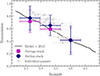 |
Fig. 1. Average transmitted flux in the rest-frame region 1041 Å < λRF,QSO < 1185 Å of the quasar spectra, as a function of the Lyα redshift, compared to the average cosmic value measured by Becker et al. (2013). Shown are the mean (purple) and median (violet) stacked spectra in three Lyα redshift intervals within 2.5 ≲ z ≲ 4.5. The uncertainties reproduce the standard deviation in each bin. In the background, there is the average transmission of individual spectra (in gray). |
2.2. Catalog of Lyα emitters
In the MAGG survey, Galbiati et al. (2023) identified 921 Lyα-emitting galaxies in the redshift range 2.8 < z < 6.6 (median z ≈ 3.91). For each galaxy, we measured its Lyα luminosity (median log[LLyα/(erg s−1)] ≈ 42.10) and projected distance from the central quasar of each field (median R ≈ 160 kpc). In particular, the fluxes are estimated using the curve of growth analysis in pseudo-narrow band images. The map of Schlafly & Finkbeiner (2011) and the extinction law of Fitzpatrick (1999) are used to correct them for the Milky Way extinction. We also derived an estimate of the redshift from their Lyα emission lines and took the red peak as a reference in the case of double-peaked line profiles. These galaxies are typically located at the low-mass end of the galaxies’ mass function at these redshifts, with M★ = 109 − 1010 M⊙, and are hosted in dark matter halos of Mh = 1010 − 1011.5 M⊙ (see, e.g., Ouchi et al. 2020; Herrero Alonso et al. 2023; Herrera et al. 2025).
We selected these galaxies following two key steps (see, Galbiati et al. 2023, for the details). First, we ran SEXTRACTOR (Bertin & Arnouts 1996) on the MUSE white-light image to identify the sources that emit bright rest-frame UV continuum. The output segmentation map was then used to extract the spectra. Using M. Fossati’s fork1 of MARZ (Hinton et al. 2016), we assigned a reliable spectroscopic redshift to 1200 sources. Second, we searched for Lyα-emitting galaxies. We subtracted all these continuum-detected sources from the MUSE datacubes and used the CUBEXTRACTOR package (Cantalupo et al. 2019) to identify emission lines of at least 27 connected voxels with signal-to-noise ratio S/N ≥ 3. In the final sample, we included all the sources detected at integrated signal-to-noise ratio ISN ≥ 7 and with line profiles that are not consistent with C IV, C III], or [O II] emitters (e.g., in case of double peaks) or other lower-redshift transitions.
3. Selection of SBLAs
In this work, we select SBLAs as Lyα forest systems with transmission −0.05 < F < 0.25 over regions of ≈ 138 km s−1 (see Pieri et al. 2014), arising from strong and blended Lyα absorption lines. Such systems have previously been studied in SDSS-III/BOSS (Pieri et al. 2014) and SDSS-IV/eBOSS spectra (Pérez-Ràfols et al. 2023; Morrison et al. 2024), for which the size of a spectral resolution element is full width at half maximum (FHWM) ≈ 138 km s−1 (approximately twice the standard SDSS spectral pixel). The original definition was calibrated at the BOSS resolution, with the adopted velocity window matching a single instrumental resolution element. This choice mitigates pixel-scale noise fluctuations while preventing multiple identifications within the same resolution element. Similarly, the adopted transmission range was empirically defined for BOSS-like noise properties, ensuring that saturated pixels affected by noise are not artificially excluded. This behavior is illustrated in the simulated spectra presented in Pieri et al. (2014). In order to enable a direct comparison with these previous works, we apply the same selection criteria to the continuum-normalized X-Shooter spectra. We then discuss how the higher spectral resolution of X-Shooter may influence the resulting SBLA sample. As a first step, since both UV-Blue (UVB) and Visible (VIS) arms have higher resolving power (see Section 2.1) than BOSS spectrographs (1650 ≲ R ≲ 2150), we convolve the X-Shooter spectra with a Gaussian filter to match the resolution of BOSS. We then re-sample the convolved spectra to a wavelength grid with constant log-spaced bins with a pixel size of 138 km s−1 by conserving the total flux (see, e.g., Carnall 2017). We chose this grid as it matches that of the BOSS spectra rebinned by a factor of ×2, as done by Pieri et al. (2014) to improve the S/N of the absorber selection. We then used the catalog of DLAs, with their respective column densities, detected in MAGG by Lofthouse et al. (2023) to mask these strong Lyα absorption systems. The same work also provides a catalog of LLSs, which we do not mask, but use to investigate their degree of overlap in the final sample of SBLAs and compare it with the predictions from Pieri et al. (2014).
We restricted our search of SBLAs to the region 1041 Å < λRF,QSO < 1185 Å in the rest-frame of the quasars as it is free from contamination of any high-order Lyman series line other than Lyα, and it is not significantly affected by continuum fitting noise by excluding Lyβ and O VI emission lines and the quasar proximity zone (see, also, Morrison et al. 2024). Finally, we selected SBLAs as systems with transmitted flux −0.05 < F < 0.25 over wavelength bins of 138 km s−1 (see Fig. 2 for an example). Finally, in defining the range of Lyα transmission used to select SBLAs, we note an important caveat. As shown in Fig. 1, the mean IGM transmission decreases by a factor of ≈2 from z = 3 to z = 4, which means that a fixed flux threshold for selecting SBLAs may include systems that satisfy the criteria due to stronger IGM absorption at higher redshift than due to their intrinsic properties. In future work, a redshift-dependent transmission threshold should be calibrated to address this limitation. A summary of the resulting samples is shown in Fig. 3, where we present the redshift distributions of the full LAE sample, the LAEs selected along the redshift path of the SBLAs, and the SBLA sample.
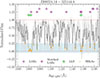 |
Fig. 2. Results of the search for SBLAs in the X-Shooter spectrum of the quasar J200324.14-325144.8. The original spectrum (light gray) has been continuum-normalized, convolved with a Gaussian filter to match the resolution of BOSS, and re-sampled into a wavelength grid with a constant bin size of 138 km s−1 (black). The pixels selected as SBLAs (orange) in the region 1041 Å < λRF,QSO < 1185 Å (that is, excluding the gray shaded regions) have a transmitted flux within the range −0.05 < F < 0.25 (blue shaded region). Known LLS are shown as green diamonds. We also show LAEs that are matched (filled purple stars) and not matched (empty purple stars) to at least one SBLA within R < 300 kpc and |Δv| ≤ 300 km s−1 in Section 4. |
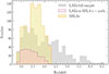 |
Fig. 3. Redshift distribution of the full LAE sample (gray), the subset of LAEs selected along the SBLA path (purple), and the complete SBLA sample (orange). |
4. The SBLA-LAE correlation
4.1. Fractions of SBLAs associated with LAEs
In Pieri et al. (2014), associations with galaxies are defined within a projected distance R ≤ 300 kpc and line-of-sight separation |Δv| ≤ 300 km s−1, and for consistency, we adopt the same definition. However, we note that the MUSE field of view extends for ≈250 kpc in radius, which implies that most of the LAEs detected are, in fact, considered when searching for associations. The region between ≈250 − 300 kpc is covered only by the four corners of the field of view, and hence it is more poorly sampled. We also note that the expected virial radius of LAEs with masses up to ≈1011 M⊙ (see, e.g., Herrero Alonso et al. 2023; Herrera et al. 2025) is ≈ 35 kpc at z ≈ 3, hence the linking length we adopted are likely probing regions that extend far beyond the CGM (the thresholds correspond to ≳8 times the virial radius, and ≈3 times the virial velocity, respectively). Fig. 2 offers an example of SBLA-LAE associations in a MAGG field.
We show in Fig. 4 (pink histogram in the left panel) and report in Table 1 the fraction of 138 km s−1 wide wavelength bins, as a function of their transmitted flux, that is found to be associated with at least one LAE within the limits above. The fractions of absorption systems identified as SBLAs (−0.05 < F < 0.25) connected to LAEs rise from ≈20 percent for wavelength bins with fluxes 0.15 < F < 0.25, to ≈25 percent for bins with 0.05 < F < 0.15 and reach ≈45 percent for bins with −0.05 < F < 0.05. Instead, only ≲10 percent of the wavelength bins with F ≳ 0.25 are associated with galaxies; that is, these bins are over three times less likely to be found near LAEs. Conversely, 211 LAEs are found in the redshift path of the wavelength bins, and ≈57 percent is associated with at least one −0.05 < F < 0.25 SBLA.
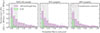 |
Fig. 4. Fraction of 138 km s−1 wavelength bins, as a function of their transmitted fluxes, that are associated with at least one LAE within a projected distance R ≤ 300 kpc and line-of-sight separation |Δv| ≤ 300 km s−1. The pink histograms show the results for all the absorption systems, while the green ones show the contribution to each flux interval of the wavelength bins that are also identified as LLSs. The gray shaded area highlights the wavelength bins with fluxes −0.05 < F < 0.25 that are identified as SBLAs. In the three panels, we show associations with the full sample of MAGG LAEs (left panel), and those above the 50 percent (middle panel) and 80 percent (right panel) completeness limit. Fractions computed with the respective completeness corrections are also shown (purple histogram). |
Statistics of LAEs and wavelength bins with F < 0.25 and Δvspec = 138 km s−1 associated with each other within |Δv| ≤ 300 km s−1 and R ≤ 300 kpc.
Next, we tested the robustness of our results against the completeness of the LAEs sample. We employed the selection function from Fossati et al. (2021) and Galbiati et al. (2023), which gives the completeness as a function of both the Lyα luminosity and the redshift of the galaxies (meaning our ability to recover LAEs in MUSE observations). To this end, we computed the fraction of LAEs associated with different wavelength bins considering only those above the 50 percent and 80 percent completeness limit, which corresponds to luminosities of log[LLyα/(erg s−1)] = 41.87 and log[LLyα/(erg s−1)] = 42 at z = 3.5, respectively. The results are displayed as pink histograms in the middle and right panels of Fig. 4. We then applied a correction by rescaling the number of LAEs found to be associated with SBLAs according to the completeness of the sample at the Lyα luminosity of the galaxies (purple histograms in Fig. 4). We observe that the completeness of the LAEs sample does not significantly impact the results. Indeed, the fraction of SBLAs with fluxes −0.05 < F < 0.05 (0.05 < F < 0.15) that are associated with galaxies corresponds to ≳30 percent (≳20 percent) even when the LAEs sample is required to be 50 percent complete.
To assess the contribution of SBLAs that arise from gas at smaller separations from LAEs, i.e., in the CGM on scales ≲3Rvir, we repeated the analysis above, but selected only associations within ≈ 100 kpc. As shown in Fig. 5, the trend observed in Fig. 4 persists also for associations with a smaller impact parameter. Wavelength bins with −0.05 < F < 0.05 are more often associated with galaxies than spectral regions at higher transmission. This indicates a tendency to find more absorbed bins in the CGM of galaxies, although the overall fraction of SBLAs associated with LAEs decreases by a factor of ≈2 compared to the analysis at R ≤ 300 kpc.
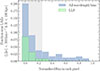 |
Fig. 5. Same as the left panel in Fig. 4, but for LAEs detected within 100 kpc of the quasar line of sight. |
Using the catalog of strong H I absorbers identified in the MAGG survey by Lofthouse et al. (2023), we next investigated the contribution of LLSs to the results we obtained. Indeed, while DLAs have already been masked, a fraction of wavelength bins with low transmitted flux identified as SBLAs can actually be strong H I absorbers, such as LLS. To quantify the degree of overlap, we derived the contribution of LLSs to the SBLAs-LAEs association by computing the fraction of wavelength bins connected to LAEs that are also LLSs, as a function of the transmitted flux (green histograms in Fig. 4). We found that of the 45 percent of wavelength bins with −0.05 < F < 0.05 associated with LAEs, ≈20 percent of them are also LLSs. As expected, such a contribution decreases steeply with increasing transmitted flux, down to ≲2 percent for bins with F > 0.05. As also noted before, this result does not vary significantly with the completeness of the LAEs sample, nor with the impact parameter used to establish the associations.
Overall, we estimate the contribution of LLSs to be on the order of ≈17.3 percent in wavelength bins with transmitted fluxes −0.05 < F < 0.25 that are identified as SBLAs. This small fraction confirms that systems at lower column density than LLSs drive the bulk of the observed associations, and hence we are not merely recovering the clustering of LAEs around optically-thick absorbers (Lofthouse et al. 2023). Conversely, all LLSs are SBLAs, as expected by the marked Lyα absorption core of these optically thick absorbers. Our analysis reaffirms the conclusion of previous authors that the incidence of LLSs in the SBLAs population is below 10 percent. Pieri et al. (2014) estimates that around ≈3.7 percent of their blended absorbers sample is optically thick, even when assuming that 100 percent of the LLSs are selected as SBLAs. Within MAGG, where we have a complete census of LLS, we confirm this result. Once we account for the correction in the incidence of LLSs discussed in Lofthouse et al. (2023) as a result of the MAGG preselection, we find that the contribution of LLSs to the sample of SBLAs is ≈4.8 percent.
4.2. The 2D cross-correlation functions
To investigate the degree to which the cross-match between SBLAs and LAEs depends on rebinning of the spectra, we reproduce the steps of Section 3 rebinning the X-Shooter spectra at their native resolution in pixels that have a width corresponding to half (that is, 69 km s−1, i.e. ≈1.7 times UVB X-shooter resolution) and twice (276 km s−1) the size of those defined by Pieri et al. (2014). We also explore how varying the limits in the projected and velocity space within which we connect the absorption systems to galaxies affects the SBLA-LAE association rate.
We compute the two-dimensional SBLA-LAE projected cross-correlation function (ξ) using the Davis & Peebles (1983) estimator2. This represents the excess probability of finding an LAE within line-of-sight separation Δvth and distance Rth from an SBLA, compared to the probability of finding an LAE within the same volume in a random place of the Universe. To reproduce the expectations for a sample of randomly distributed SBLAs and LAEs, we connected the absorbers identified in the spectrum of a given quasar with LAEs detected in a field randomly extracted among those centered on the other quasars (as done in previous MAGG papers, e.g., Galbiati et al. 2023). We then bootstrapped 1,000 times over the fields and took the median values of the resulting distribution. The cross-correlation functions that we obtained with this method are shown in Fig. 6.
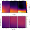 |
Fig. 6. Two-dimensional LAE-absorber cross-correlation functions, ξ. Upper panels: Cross-correlation functions for systems with −0.05 < F < 0.25. The linking velocity window, Δvth, and projected separation, ΔRth, vary along the vertical and horizontal axis, respectively. Each of the three panels shows the results for SBLAs identified in quasar spectra with a pixel size of Δvspec = 69 km s−1 (left panel), 138 km s−1 (middle panel), and 276 km s−1 (right panel). Line-of-sight separations Δvth < Δvspec are masked. Lower panels: Cross-correlation functions between LAEs and systems with F > 0.25. Note the different limits on the ξ color scale. |
In the upper panels, we computed the cross-correlation by searching for SBLAs (−0.05 < F < 0.25) in the quasar spectra rebinned in the three different pixel sizes introduced above. In the lower panel, we show the cross-correlations obtained by linking to LAEs the pixels with F > 0.25. To ensure a consistent comparison, the line-of-sight velocity separation in all panels is computed as a multiple of the spectral pixel size. Values at impact parameters ≳ 250 kpc should be treated with caution, as we are approaching the edge of the MUSE field of view and thus have a sparser sample.
Examining Fig. 6, we notice that LAEs are more likely to be found near SBLAs compared to random regions, with a clear preference to cluster towards low velocities and small impact parameters. Conversely, there is no obvious clustering of LAEs in spectral bins with F > 0.25, i.e., near non-SBLAs. The distribution of LAEs around these spectral bins is consistent at any separation with ξ ≈ 0, that is, with a random distribution. Thus, it is more likely that systems with F > 0.25 arise from IGM gas. Both the amplitude and the radial profile of the clustering of LAEs around SBLAs vary with the size of the spectral pixels. The excess of LAEs is larger around the SBLAs identified in spectra with increasing Δvspec and reaches its maximum around Δvspec = 276 km s−1. We explicitly tested that further increasing the spectral pixel size results in a roughly constant cross-correlation amplitude (with variations of ≲15%). Although the SBLA fraction at Δvspec = 276 km s−1 has dropped by ≈50% compared to that at 69 km s−1, this observed cross-correlation trend is driven by the survival of SBLAs made of smaller ones selected at lower Δvspec. In other words, at large spectral pixel sizes, the observed cross-correlation amplitude reflects the persistence of more extended structures rather than the appearance of new ones. Finally, we note that the scale on which we detect a significant LAE-SBLA correlation, R ≲ 150 kpc, extends beyond the typical virial radius expected for halos hosting LAEs (≈ 35 kpc). This implies that part of the signal may arise from the CGM of neighboring clustered galaxies rather than only the halo of an individual LAE itself.
4.3. The LAE luminosity function near SBLAs
A complementary approach to studying the projected correlation function to connect LAEs and SBLAs is to examine the LAE luminosity function in regions that host SBLAs. Once again, we consider SBLAs as a function of the size of the spectral pixels and statistically study how LAEs distribute in their surroundings as a function of the Lyα luminosity. Following the steps detailed in Fossati et al. (2021) and Galbiati et al. (2023), we computed the Lyα luminosity functions of LAEs identified within |Δv| ≤ 300 km s−1 and R ≤ 300 kpc around SBLAs and fitted them with a parametric Schechter (1976) function. The results are shown in Fig. 7 and reported in Table 2. These are compared with the luminosity functions of LAEs representative of the field from Galbiati et al. (2023), as well as those identified around strong H I absorbers (LLSs and DLAs, log(NHI/cm−2) ≳ 17) from Lofthouse et al. (2023).
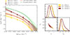 |
Fig. 7. Lyα luminosity functions of the LAEs associated with SBLAs within R ≤ 300 kpc and |Δv| ≤ 300 km s−1. Left panel: Lyα luminosity functions of the LAEs associated with SBLAs identified in the quasar spectra binned to Δvspec = 69, 138, 276 km s−1 (from light to dark colors). For comparison, we also show the luminosity function expected for LAEs in the field (red, Galbiati et al. 2023) and for those found around strong H I absorbers (green, Lofthouse et al. 2023). Right panel: Posterior distribution of the α and L★ free parameters obtained fitting the luminosities functions with a Schechter (1976). The contours mark the confidence intervals corresponding to 1σ and 2σ. |
Best-fit Schechter function parameters of the luminosity functions of LAEs associated with SBLAs identified in spectra with different Δvspec.
We find that the luminosity functions of LAEs around SBLAs have a shape similar to those derived in MAGG, indicating no notable excess of either bright or faint LAEs. The main differences appear in normalization, which traces the amplitude of the galaxy overdensity. This normalization increases with the spectral pixel size used to define SBLAs, suggesting that Δvspec plays a significant role in the interpretation of the nature of these absorption systems. In particular, SBLAs identified with Δvspec = 69 km s−1 show the lowest normalization, even lower than that of field LAEs. A possible scenario is that a significant fraction of these absorbers are pinpointing volumes that are not occupied by the LAEs detected in MAGG, a characteristic that could suggest a larger contribution from the IGM rather than the CGM at these velocity scales. This may also result from contamination of the SBLAs sample arising from noise fluctuations that can affect the purity of the selection for relatively high transmissions −0.05 < F < 0.25. Selecting stronger absorbers (e.g., −0.05 < F < 0.15 and −0.05 < F < 0.05) mitigates this effect and results in normalizations that are up to ≈0.25 dex higher, strongly suggesting that the contribution of the CGM gas can be significant at these fluxes even for small Δvspec. Finally, a combination of this effect and the contribution of gas located on scales larger than the typical CGM can also be considered a plausible interpretation. For Δvspec = 138 km s−1, the luminosity function closely matches that of field LAEs and is thus consistent with SBLAs tracing the CGM of the galaxies. Finally, the strongest overdensity is observed for Δvspec = 276 km s−1, where the normalization exceeds the field, but is still significantly lower compared to the largest overdensity of LAEs observed around stronger H I absorbers. These SBLAs may therefore trace regions populated by a larger number density of galaxies where it is more likely that a significant contribution to the observed absorption arises from overlapping halos. In such environments, the circumgalactic gas associated with neighboring systems can produce absorption components that are close to the velocity space. If not individually resolved, their superimposition may appear as a single broader absorption feature.
5. Discussion and conclusions
Analysis of the link between LAEs and spectral bins with varying transmission in MAGG fields shows that wavelength bins with F < 0.25, selected as SBLAs, are found more frequently near LAEs than those at F > 0.25. The correlation between SBLAs and galaxies also depends on the size of the spectral bin, being the strongest for Δvspec = 276 km s−1 and for small impact parameters, R ≲ 150 kpc. From these results, we conclude that SBLAs identify regions of high optical depth that differ from random IGM regions, are preferentially occupied by star-forming galaxies, and do not overlap significantly with LLSs.
The findings of our LAE analysis share similarities with those of studies conducted in the vicinity of LBGs. Pieri et al. (2014) studied associations with LBGs, finding that SBLAs with F < 0.25 reside near an LBG ≈60 percent of the time, in excess compared to a random distribution. Associations between LBGs and regions of enhanced absorption are also found in large spectroscopic surveys of galaxies in quasar fields. Rudie et al. (2012) investigated the correlation between H I absorbers in the range 1012 ≤ NH I/cm−2 ≤ 1021 and LBGs with z ≈ 2 − 3. Hydrogen absorbers with NH I/cm−2 ≳ 1014.5 cluster preferentially within ≈ 300 kpc and ≈ 300 km s−1 of galaxies, a trend that is not observed at a lower column density. These authors further estimate that circumgalactic gas can account for ≈50 percent of all systems with NH I/cm−2 ≳ 1015.5, a value in line with the inferred column density of SBLAs (Morrison et al. 2024). Similar conclusions are reached by Rakic et al. (2012), who examined the correlation between LBGs and H I optical depth in the same sample of LBGs studied by Rudie et al. (2012). Regions with elevated optical depth, τLyα > 0.1, are found closer to galaxies than random regions. Circumgalactic gas within ≈ 100−200 kpc contributes to absorption with optical depth τLyα ≳ 1, corresponding to column densities NH I/cm−2 ≳ 1014 and a transmitted flux similar to the one that defines SBLAs.
Although not strictly quantitative, this comparison underscores similarities between LBGs and our findings with LAEs: ≈40 − 60 percent of SBLAs are identifiable with circumgalactic gas within ≈ 300 kpc and ≈ 300 km s−1 of star-forming galaxies. Exploring stacked quasar spectra around z ≈ 3 − 4 LAEs, Muzahid et al. (2021) found that the H I optical depth is significantly higher within LOS separations of |Δv|≲ 500 km s−1 from the galaxies compared to random regions in the Universe (see, also, Matthee et al. 2024). In addition, they reported a peak at F < 0.05 in the flux distribution of pixels within ±100 km s−1 of the LAEs, in agreement with the excess of low-transmission absorbers we observe in Fig. 5.
However, LAEs and LBGs are only partially overlapping populations: the typical halo mass of LBGs is inferred around ≈1011.5 − 1012 M⊙ (Bielby et al. 2013; Rakic et al. 2013) and the mass of LAEs selected by typical IFS observations spans a luminosity-dependent range of Mh ≈ 1010 − 1011.5 M⊙ (Herrero Alonso et al. 2023). Recent theoretical work by Muñoz Santos et al. (2025) suggests a connection between the velocity scale over which SBLAs are found and the halo mass of the associated galaxies. According to the cross-correlations in Fig. 6, a stronger signal over velocity scales ≳ 250 km s−1 is to be expected for halos with Mh ≳ 1011 M⊙, with a peak at Mh ≈ 1011.5 M⊙. The LAEs in MAGG are bright enough (log[LLyα/(erg s−1)] ≳ 41.8; see Fig. 7) to enter the intermediate (⟨log(LLyα/(erg s−1)]⟩ = 41.64) and high-luminosity range (⟨log[LLyα/(erg s−1)]⟩ = 42.34) according to the definition in the clustering analysis by Herrero Alonso et al. (2023). The inferred mass is therefore around Mh ≈ 1011.2 M⊙, which is just a factor ≈2 smaller than the peak value predicted by Muñoz Santos et al. (2025). Given the wide distributions reported in their figure B.1, this small discrepancy does not imply a tension. Expanded samples should next explore the dependence of the LAE-SBLA association on luminosity as a test of the predicted halo mass range. We also note that observational selection effects limit the detection of LAEs to relatively luminous galaxies. As a result, our analysis likely traces only a subset of the full galaxy population associated with SBLAs, namely the brighter Lyα-emitting galaxies (with a 50% completeness limit corresponding to log[LLyα/(erg s−1)] ≈ 41.87; see Fossati et al. 2021; Galbiati et al. 2023) accessible to our survey. Other galaxies, including systems with weak or absent Lyα emission, may remain undetected. Therefore, the lack of a detected association for the remaining absorbers does not necessarily imply the absence of circumgalactic gas.
In conclusion, our analysis confirms that a significant fraction (≈40 percent) of SBLAs are associated with circumgalactic gas in LAEs, reaffirming that strong blended absorbers can pinpoint the CGM of high redshift galaxies at intermediate column densities in between the Lyα forest and the optically-thick LLSs (Rudie et al. 2012; Morrison et al. 2024). We also find that the LAE-SBLA cross-correlation is strongly sensitive to the spectral binning used to identify these absorbers, consistent with trends suggested by recent observational (Pérez-Ràfols et al. 2023; Morrison et al. 2024) and theoretical (Muñoz Santos et al. 2025) studies. Thus, the current framework appears to be effective in linking absorbers to halos and galaxies, although it has only been tested at z ≲ 3. However, further work is needed to quantify how the choice of selection parameters influences the SBLA-halo association and, in particular, there is room to test how optimizing the flux threshold as a function of both redshift and spectral binning would improve the selection and characterization of SBLAs, especially at z ≳ 3.
Acknowledgments
We thank the anonymous referee for carefully reading the paper and for providing useful suggestions that helped improve the manuscript. This paper uses data from the MAGG survey, based on observations collected at the European Organisation for Astronomical Research in the Southern Hemisphere under ESO programme IDs 197.A-0384, 065.O-0299, 067.A-0022, 068.A-0461, 068.A-0492, 068.A-0600, 068.B-0115, 069.A-0613, 071.A-0067, 071.A-0114, 073.A-0071, 073.A-0653, 073.B-0787, 074.A-0306, 075.A-0464, 077.A-0166, 080.A-0482, 083.A-0042, 091.A-0833, 092.A-0011, 093.A-0575, 094.A-0280, 094.A-0131, 094.A-0585, 095.A-0200, 096.A-0937, 097.A-0089, 099.A-0159, 166.A-0106, 189.A-0424, 0109.A-0559. This study is supported by the Italian Ministry for Research and University (MUR) under Grant ‘Progetto Dipartimenti di Eccellenza 2023-2027’ (BiCoQ). MG also acknowledges support by Progetto FARE 2020 Svelare i nodi massicci della CosmicWeb ID 2021-NAZ-0326/PER. This research used Astropy (http://www.astropy.org), a community-developed core Python package for Astronomy (Astropy Collaboration 2013, 2018, 2022), NumPy (Harris et al. 2020), SciPy (Virtanen et al. 2020), Matplotlib (Hunter 2007).
References
- Astropy Collaboration (Robitaille, T. P., et al.) 2013, A&A, 558, A33 [NASA ADS] [CrossRef] [EDP Sciences] [Google Scholar]
- Astropy Collaboration (Price-Whelan, A. M., et al.) 2018, AJ, 156, 123 [Google Scholar]
- Astropy Collaboration (Price-Whelan, A. M., et al.) 2022, ApJ, 935, 167 [NASA ADS] [CrossRef] [Google Scholar]
- Bacon, R., Accardo, M., Adjali, L., et al. 2010, in Ground-based and Airborne Instrumentation for Astronomy III, eds. I. S. McLean, S. K. Ramsay, & H. Takami, SPIE Conf. Ser., 7735, 773508 [Google Scholar]
- Becker, G. D., Hewett, P. C., Worseck, G., & Prochaska, J. X. 2013, MNRAS, 430, 2067 [Google Scholar]
- Bertin, E., & Arnouts, S. 1996, A&AS, 117, 393 [NASA ADS] [CrossRef] [EDP Sciences] [Google Scholar]
- Bielby, R., Hill, M. D., Shanks, T., et al. 2013, MNRAS, 430, 425 [CrossRef] [Google Scholar]
- Cantalupo, S., Pezzulli, G., Lilly, S. J., et al. 2019, MNRAS, 483, 5188 [Google Scholar]
- Carnall, A. C. 2017, arXiv e-prints [arXiv:1705.05165] [Google Scholar]
- Davis, M., & Peebles, P. J. E. 1983, ApJ, 267, 465 [Google Scholar]
- Dutta, R., Fumagalli, M., Fossati, M., et al. 2020, MNRAS, 499, 5022 [CrossRef] [Google Scholar]
- Dutta, R., Fumagalli, M., Fossati, M., et al. 2021, MNRAS, 508, 4573 [NASA ADS] [CrossRef] [Google Scholar]
- Fitzpatrick, E. L. 1999, PASP, 111, 63 [Google Scholar]
- Fossati, M., Fumagalli, M., Lofthouse, E. K., et al. 2021, MNRAS, 503, 3044 [NASA ADS] [CrossRef] [Google Scholar]
- Fumagalli, M., Prochaska, J. X., Kasen, D., et al. 2011, MNRAS, 418, 1796 [CrossRef] [Google Scholar]
- Fumagalli, M., O’Meara, J. M., Prochaska, J. X., & Worseck, G. 2013, ApJ, 775, 78 [Google Scholar]
- Fumagalli, M., O’Meara, J. M., & Prochaska, J. X. 2016, MNRAS, 455, 4100 [NASA ADS] [CrossRef] [Google Scholar]
- Galbiati, M., Fumagalli, M., Fossati, M., et al. 2023, MNRAS, 524, 3474 [NASA ADS] [CrossRef] [Google Scholar]
- Galbiati, M., Dutta, R., Fumagalli, M., Fossati, M., & Cantalupo, S. 2024, A&A, 690, A7 [NASA ADS] [CrossRef] [EDP Sciences] [Google Scholar]
- Harris, C. R., Millman, K. J., Van Der Walt, S. J., et al. 2020, Nature, 585, 357 [NASA ADS] [CrossRef] [Google Scholar]
- Herrera, D., Gawiser, E., Benda, B., et al. 2025, ApJ, 988, L57 [Google Scholar]
- Herrero Alonso, Y., Miyaji, T., Wisotzki, L., et al. 2023, A&A, 671, A5 [NASA ADS] [CrossRef] [EDP Sciences] [Google Scholar]
- Hinton, S. R., Davis, T. M., Lidman, C., Glazebrook, K., & Lewis, G. F. 2016, Astron. Comput., 15, 61 [Google Scholar]
- Hunter, J. D. 2007, Comput. Sci. Eng., 9, 90 [NASA ADS] [CrossRef] [Google Scholar]
- Khare, P., Kulkarni, V. P., Péroux, C., et al. 2007, A&A, 464, 487 [NASA ADS] [CrossRef] [EDP Sciences] [Google Scholar]
- Lofthouse, E. K., Fumagalli, M., Fossati, M., et al. 2020, MNRAS, 491, 2057 [NASA ADS] [CrossRef] [Google Scholar]
- Lofthouse, E. K., Fumagalli, M., Fossati, M., et al. 2023, MNRAS, 518, 305 [Google Scholar]
- López, S., D’Odorico, V., Ellison, S. L., et al. 2016, A&A, 594, A91 [NASA ADS] [CrossRef] [EDP Sciences] [Google Scholar]
- Lynds, R. 1971, ApJ, 164, L73 [NASA ADS] [CrossRef] [Google Scholar]
- Matthee, J., Golling, C., Mackenzie, R., et al. 2024, MNRAS, 529, 2794 [Google Scholar]
- Morrison, S., Som, D., Pieri, M. M., Pérez-Ràfols, I., & Blomqvist, M. 2024, MNRAS, 532, 32 [Google Scholar]
- Muñoz Santos, D., Pieri, M. M., Nelson, D., et al. 2025, arXiv e-prints [arXiv:2507.08940] [Google Scholar]
- Muzahid, S., Schaye, J., Cantalupo, S., et al. 2021, MNRAS, 508, 5612 [NASA ADS] [CrossRef] [Google Scholar]
- Ouchi, M., Ono, Y., & Shibuya, T. 2020, ARA&A, 58, 617 [Google Scholar]
- Pérez-Ràfols, I., Pieri, M. M., Blomqvist, M., et al. 2023, MNRAS, 524, 1464 [Google Scholar]
- Péroux, C., Dessauges-Zavadsky, M., Kim, T., McMahon, R. G., & D’Odorico, S. 2002, Ap&SS, 281, 543 [Google Scholar]
- Pieri, M. M., Frank, S., Weinberg, D. H., Mathur, S., & York, D. G. 2010, ApJ, 724, L69 [Google Scholar]
- Pieri, M. M., Mortonson, M. J., Frank, S., et al. 2014, MNRAS, 441, 1718 [Google Scholar]
- Planck Collaboration I. 2016, A&A, 594, A1 [NASA ADS] [CrossRef] [EDP Sciences] [Google Scholar]
- Prochaska, J. X., O’Meara, J. M., & Worseck, G. 2010, ApJ, 718, 392 [Google Scholar]
- Rahmati, A., Pawlik, A. H., Raičević, M., & Schaye, J. 2013, MNRAS, 430, 2427 [NASA ADS] [CrossRef] [Google Scholar]
- Rakic, O., Schaye, J., Steidel, C. C., & Rudie, G. C. 2012, ApJ, 751, 94 [NASA ADS] [CrossRef] [Google Scholar]
- Rakic, O., Schaye, J., Steidel, C. C., et al. 2013, MNRAS, 433, 3103 [Google Scholar]
- Rauch, M. 1998, ARA&A, 36, 267 [Google Scholar]
- Rudie, G. C., Steidel, C. C., Trainor, R. F., et al. 2012, ApJ, 750, 67 [NASA ADS] [CrossRef] [Google Scholar]
- Schechter, P. 1976, ApJ, 203, 297 [Google Scholar]
- Schlafly, E. F., & Finkbeiner, D. P. 2011, ApJ, 737, 103 [Google Scholar]
- Tumlinson, J., Peeples, M. S., & Werk, J. K. 2017, ARA&A, 55, 389 [Google Scholar]
- Tytler, D. 1982, Nature, 298, 427 [NASA ADS] [CrossRef] [Google Scholar]
- Vernet, J., Dekker, H., D’Odorico, S., et al. 2011, A&A, 536, A105 [NASA ADS] [CrossRef] [EDP Sciences] [Google Scholar]
- Virtanen, P., Gommers, R., Oliphant, T. E., et al. 2020, Nat. Methods, 17, 261 [Google Scholar]
- Wolfe, A. M., Gawiser, E., & Prochaska, J. X. 2005, ARA&A, 43, 861 [NASA ADS] [CrossRef] [Google Scholar]
In this formalism, the cross-correlation is defined as 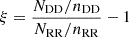 , where NDD, and NRR are the number of galaxy-absorber pairs identified in the data and in the random sample, respectively, within each separation interval, while nDD, and nRR account for the total number of pairs in the two samples.
All Tables
Statistics of LAEs and wavelength bins with F < 0.25 and Δvspec = 138 km s−1 associated with each other within |Δv| ≤ 300 km s−1 and R ≤ 300 kpc.
Best-fit Schechter function parameters of the luminosity functions of LAEs associated with SBLAs identified in spectra with different Δvspec.
All Figures
|
Fig. 1. Average transmitted flux in the rest-frame region 1041 Å < λRF,QSO < 1185 Å of the quasar spectra, as a function of the Lyα redshift, compared to the average cosmic value measured by Becker et al. (2013). Shown are the mean (purple) and median (violet) stacked spectra in three Lyα redshift intervals within 2.5 ≲ z ≲ 4.5. The uncertainties reproduce the standard deviation in each bin. In the background, there is the average transmission of individual spectra (in gray). |
| In the text | |
|
Fig. 2. Results of the search for SBLAs in the X-Shooter spectrum of the quasar J200324.14-325144.8. The original spectrum (light gray) has been continuum-normalized, convolved with a Gaussian filter to match the resolution of BOSS, and re-sampled into a wavelength grid with a constant bin size of 138 km s−1 (black). The pixels selected as SBLAs (orange) in the region 1041 Å < λRF,QSO < 1185 Å (that is, excluding the gray shaded regions) have a transmitted flux within the range −0.05 < F < 0.25 (blue shaded region). Known LLS are shown as green diamonds. We also show LAEs that are matched (filled purple stars) and not matched (empty purple stars) to at least one SBLA within R < 300 kpc and |Δv| ≤ 300 km s−1 in Section 4. |
| In the text | |
|
Fig. 3. Redshift distribution of the full LAE sample (gray), the subset of LAEs selected along the SBLA path (purple), and the complete SBLA sample (orange). |
| In the text | |
|
Fig. 4. Fraction of 138 km s−1 wavelength bins, as a function of their transmitted fluxes, that are associated with at least one LAE within a projected distance R ≤ 300 kpc and line-of-sight separation |Δv| ≤ 300 km s−1. The pink histograms show the results for all the absorption systems, while the green ones show the contribution to each flux interval of the wavelength bins that are also identified as LLSs. The gray shaded area highlights the wavelength bins with fluxes −0.05 < F < 0.25 that are identified as SBLAs. In the three panels, we show associations with the full sample of MAGG LAEs (left panel), and those above the 50 percent (middle panel) and 80 percent (right panel) completeness limit. Fractions computed with the respective completeness corrections are also shown (purple histogram). |
| In the text | |
|
Fig. 5. Same as the left panel in Fig. 4, but for LAEs detected within 100 kpc of the quasar line of sight. |
| In the text | |
|
Fig. 6. Two-dimensional LAE-absorber cross-correlation functions, ξ. Upper panels: Cross-correlation functions for systems with −0.05 < F < 0.25. The linking velocity window, Δvth, and projected separation, ΔRth, vary along the vertical and horizontal axis, respectively. Each of the three panels shows the results for SBLAs identified in quasar spectra with a pixel size of Δvspec = 69 km s−1 (left panel), 138 km s−1 (middle panel), and 276 km s−1 (right panel). Line-of-sight separations Δvth < Δvspec are masked. Lower panels: Cross-correlation functions between LAEs and systems with F > 0.25. Note the different limits on the ξ color scale. |
| In the text | |
|
Fig. 7. Lyα luminosity functions of the LAEs associated with SBLAs within R ≤ 300 kpc and |Δv| ≤ 300 km s−1. Left panel: Lyα luminosity functions of the LAEs associated with SBLAs identified in the quasar spectra binned to Δvspec = 69, 138, 276 km s−1 (from light to dark colors). For comparison, we also show the luminosity function expected for LAEs in the field (red, Galbiati et al. 2023) and for those found around strong H I absorbers (green, Lofthouse et al. 2023). Right panel: Posterior distribution of the α and L★ free parameters obtained fitting the luminosities functions with a Schechter (1976). The contours mark the confidence intervals corresponding to 1σ and 2σ. |
| In the text | |
Current usage metrics show cumulative count of Article Views (full-text article views including HTML views, PDF and ePub downloads, according to the available data) and Abstracts Views on Vision4Press platform.
Data correspond to usage on the plateform after 2015. The current usage metrics is available 48-96 hours after online publication and is updated daily on week days.
Initial download of the metrics may take a while.