


| Issue |
A&A
Volume 711, July 2026
|
|
|---|---|---|
| Article Number | A244 | |
| Number of page(s) | 14 | |
| Section | The Sun and the Heliosphere | |
| DOI | https://doi.org/10.1051/0004-6361/202558403 | |
| Published online | 17 July 2026 | |
Recurrent release of coronal density structures during the rising phase of solar cycle 25
1
INAF, Catania Astrophysical Observatory, Via S. Sofia 78, I-95123 Catania, Italy
2
INAF, Turin Astrophysical Observatory, Via Osservatorio 20, I-10025 Pino, Torinese (TO), Italy
3
Space Science Division, Naval Research Laboratory, Washington, DC 20375, USA
4
INAF, Institute of Space Astrophysics and Cosmic Physics of Milan, Via Alfonso Corti 12, I-20133 Milano, Italy
5
IUSS – Scuola Universitaria Superiore, Piazza della Vittoria, 15, I-27100 Pavia, Italy
6
INAF – Astronomical Observatory of Capodimonte, Salita Moiariello 16, I-80131 Napoli, Italy
7
University of Florence, Department of Physics and Astronomy, Via Giovanni Sansone 1, I-50019 Sesto, Fiorentino, Italy
8
National Research Council, Institute for Photonics and Nanotechnologies, Via Trasea 7, I-35131 Padova, Italy
9
Institute of Physics, University of Graz, Universitätsplatz 5, 8010 Graz, Austria
10
INAF, Astronomical Observatory of Trieste, Localitá Basovizza 302, I-34149 Trieste, Italy
11
INAF, Astrophysical Observatory of Arcetri, Largo Enrico Fermi 5, I-50125 Firenze, Italy
★ Corresponding author: This email address is being protected from spambots. You need JavaScript enabled to view it.
Received:
4
December
2025
Accepted:
7
June
2026
Abstract
Aims. We investigate the main physical characteristics and outward propagation in the solar corona of small-scale coronal transients detected during the rising phase of solar activity cycle 25. They were observed with the Metis coronagraph on Solar Orbiter when the spacecraft was at perihelion, 0.29 au, on October 12, 2022. We compare the results with the Metis observations obtained in February 2021, when Solar Orbiter was at 0.52 au, which revealed intermittent quasi-periodic small-scale structures propagating in a still relatively quiescent corona, between 3.10 and 5.70 R⊙.
Methods. The method we adopted is based on the construction of height-time maps of total brightness detected in the Metis white-light channel for three selected angular sectors of the solar corona. We carried out a spectral analysis of the temporal series of the total brightness obtained as a function of heliocentric distance and solar latitude by applying the Lomb-Scargle procedure.
Results. Propagating plasma density inhomogeneities are observed above the solar limb within the altitude range 1.76–3.10 R⊙, in fairly quiet coronal regions that correspond to segments of the warped streamer belt, which is highly inclined relative to the solar equator. This is expected in the ascending-maximum phase of the solar activity cycle. These structures are characterized by radial and transverse sizes of 30–75 ± 8 Mm (0.04–0.10 ± 0.01 R⊙) and 30–50 ± 8 Mm (0.04–0.07 ± 0.01 R⊙), respectively. Most of them are fast-evolving structures that rapidly change in shape, dimension, and brightness on a timescale even as short as the observation cadence. The enhanced density structures move into the ambient slow wind with a mean velocity of about 240 ± 70 km s−1. They are intermingled with downflows that mainly originate in the range of heliocentric distances 2.0–2.5 R⊙ and flow inward with speeds ranging over a wide interval, from about 35 ± 1 km s−1 to about 200 ± 15 km s−1. The coronal emission integrated over specific latitude intervals of 10° – 20° is characterized by a well-defined periodicity of 42 min. The observations suggest that any dynamical process causing the presence and release of the density structures coherently acts in specific areas according to some periodic clock.
Conclusions. The results show that propagating density structures are already present in the corona at 1.76 R⊙ (the internal occulter edge of the coronagraph). Their concentration in the range of heliocentric distance between 2.0 and 2.4 R⊙, that is, inside well-defined regions corresponding to streamer belt segments running almost parallel to the limb, is higher. Numerous dark structures moving inward are also present, mainly at the interface between open and closed magnetic lines at the streamer borders. The coronal plasma ejecta is likely released by processes of magnetic reconnection that are triggered in specific locations along the streamer borders in a period of 42 minutes. The driver of the quasi-periodic release of the density structures might be related to the photospheric convective motions and associated emergence of magnetic flux tubes, and also to the propagation of shocks at the boundary of the convection cells.
Key words: magnetohydrodynamics (MHD) / Sun: corona / solar wind
© The Authors 2026
 Open Access article, published by EDP Sciences, under the terms of the Creative Commons Attribution License (https://creativecommons.org/licenses/by/4.0), which permits unrestricted use, distribution, and reproduction in any medium, provided the original work is properly cited.
This article is published in open access under the Subscribe to Open model. This email address is being protected from spambots. You need JavaScript enabled to view it. to support open access publication.
1. Introduction
The continuous monitoring of the outer solar corona that was initiated with the dedicated set of instruments on board the Solar and Heliospheric Observatory (SOHO; Domingo et al. 1995) spacecraft launched at the end of 1995, was carried out and complemented with the coronagraphs of the Solar TErrestrial RElations Observatory (STEREO; Kaiser 2005) mission, launched in October 2006, and more recently, with the Multi Element Telescope for Imaging and Spectroscopy (Metis; Antonucci et al. 2020b; Fineschi et al. 2020) coronagraph of the Solar Orbiter (Müller et al. 2020) mission, launched in February 2020. This wealth of coronal observations provides a clear picture of the solar wind, which is the incessant outflow of solar plasma that shapes the heliosphere.
The spectroscopic measurements obtained with the SOHO Ultraviolet Coronagraph Spectrometer (UVCS; Kohl et al. 1995) allowed us to investigate the dynamics of the solar wind directly in the corona above 1.5 R⊙ for the first time by detecting the ultraviolet coronal emission in lines that in an expanding fluid are dimmed to an extent that depends on the outflow speed (Hyder & Lites 1970; Withbroe et al. 1982). The UVCS observations were performed throughout various phases of solar cycle 23 in coronal regions of open magnetic field lines characterized by different expansion factors that modulate the wind velocity, spanning from the core of coronal holes, the source of the fast wind, to the hole edges (see reviews by Antonucci 2006; Cranmer et al. 2017; Antonucci et al. 2020a, and references therein). In the simplest large-scale magnetic configuration of the solar corona, typical of the solar minimum, the equatorial streamer belt, and farther out, the coronal-heliospheric current sheet forming at the streamer cusp, are embedded in the slow wind. This result has been confirmed by observations (Romoli et al. 2021; Antonucci et al. 2023) of the Metis coronagraph on board Solar Orbiter.
Throughout almost three solar cycles, the white-light Large Angle and Spectrometric Coronagraphs (LASCO; Brueckner et al. 1995) on board SOHO have been continuously monitoring the transient events of coronal plasma release in a field of view within 2.0–30 R⊙. The events range from huge coronal mass ejections to the medium-size blobs that detach at the tip of coronal streamers, which were discovered by Sheeley et al. (1997) (see also reviews by Wang et al. 2000; Wang 2012). The LASCO investigations of the solar corona have recently been reviewed by Howard et al. (2023).
In the past two decades, the images provided by the two coronagraphs COR1 (Thompson et al. 2003) and COR2 (Howard et al. 2008) on board STEREO, extending from 1.5 to 15 R⊙, highlighted an even wider variety of coronal transients: smaller-scale quasi-periodic density structures, ejected with periodicities varying from minutes to several hours (see the review by Viall et al. 2021, and reference therein). The wide range of coronal transients, from the large coronal mass ejections to the small-scale plasmoids, poses questions about the extent of the contribution during the solar cycle of such transients to the solar wind in terms of mass and magnetic flux, of the identification of the processes that generate and propagate them, and of the origin itself of the meso-scale features observed in the heliosphere. These might in principle have either a solar origin or might be formed during the plasma propagation in the heliosphere (see, e.g., the review by Kepko et al. 2024).
The Metis coronagraph on Solar Orbiter resumed the study of the outflows of the solar wind and coronal transients early in solar cycle 25, during the quiescent phase of the Sun. This was achieved by observing the corona with an unprecedented spatial (down to ≃4000 km at minimum perihelion) and temporal resolution (down to 1 s for fixed-polarization sequences) over an altitude range from 1.7 to 9.0 R⊙ (Antonucci et al. 2020b) because the field of view (FoV) varies with the helio-distance along the spacecraft orbit and throughout the mission.
Early in the mission, on February 22, 2021, intermittent quasi-periodic small-scale structures propagating outward in a FoV within 3.1–5.7 R⊙ were detected in a latitude range from 15° N to 30° S. They embedded the almost equatorial streamer belt and its associated heliospheric current sheet. These structures, with radial and transverse dimensions of about 500 Mm (0.7 R⊙) and 40 Mm (0.06 R⊙), respectively, were released with a cadence of about 80 min and propagated outward at an average speed of 240 ± 40 km s−1 (Ventura et al. 2023, hereafter Paper I) in an ambient solar wind flowing at a speed of 175–230 km s−1 in the slow wind belt, as derived from the HI Lyα emission that undergoes Doppler dimming in an expanding atmosphere (Antonucci et al. 2023). Hence, they appeared to propagate more rapidly than the solar wind in the region surrounding the streamer belt. These results confirmed previous observations of transient density fluctuations detected in the solar corona (above 2.5 R⊙) with periodicities of 80–90 min (Viall & Vourlidas 2015) and in the heliosphere (e.g., Kepko et al. 2016; Di Matteo et al. 2019; Viall et al. 2021; Kepko et al. 2024). According to Paper I, the quasi-periodic density inhomogeneities detected by Metis in February 2021 are formed and released below or at the lower boundary of the FoV at 3.10 R⊙. This conclusion is supported by the results of Jones & Davila (2009), who explored the corona in the range 1.5–3.5 R⊙ with the STEREO-COR1 coronagraph, finding periodic density enhancements propagating at 240 km s−1, and by the results of Viall & Vourlidas (2015), who studied the corona in a region from 2.5 to 5 R⊙ with the STEREO-COR2 coronagraph. Coronal density transients with a periodicity of about 80 min were also detected in the inner corona in the range 1.5–2.5 R⊙ by studying Type IV radio emission (Pylaev et al. 2017).
The process of the release and ejection of coronal plasma can either be associated with the opening of closed magnetic flux or with interchange reconnection between open and closed magnetic field lines. These interpretations are related to the fact that in the simplest large-scale magnetic configuration of the solar corona at solar minimum, the latitudinal belt in which the small-scale density structures and the slow wind propagate corresponds to the latitudinal distribution of the network of separatrix and quasi-separatrix layers in corona, the so-called S-web (Antiochos et al. 2012), as discussed in Antonucci et al. (2023) and in Paper I. In some circumstances, the release and outflow of these small plasmoids are associated with the concomitant or subsequent formation of transient structures that collapse back toward the Sun. Inflows can appear as inward-moving density enhancements or depletions, as reported, for instance, by Sheeley & Wang (2007), Sanchez-Diaz et al. (2017) and Alzate et al. (2024). Following the interpretation proposed by Wang (2024), these inflows are triggered by the pinch-off of outward-expanding helmet-streamer loops. This occurs where the density in a loop is very low, so the inflows tend to be dark, although they may brighten as they sweep up ambient material during their collapse. No such features were detected in the observations of Metis in February 2021 (Paper I).
We here investigate the physical characteristics, height of formation, and early propagation of the small-scale coronal transients further on the basis of a sequence of white-light coronal images acquired with Metis during the close approach of Solar Orbiter to the Sun on October 12, 2022, when the spacecraft at perihelion was at 0.29 au.
Since February 2021, the global corona topology significantly changed from a configuration dominated by a quasi-equatorial streamer belt (Paper I) to a configuration characterized by a highly warped coronal heliospheric current sheet. Hence, the line of sight of the coronagraph, which during solar minimum lay roughly along the heliospheric current sheet, assumed an almost perpendicular direction relative to the heliospheric current sheet during the ascending phase of solar activity. This is the most favorable condition for observations of density structures flowing outward from the streamer belt and adjacent regions and of their spatial distribution (e.g., Sanchez-Diaz et al. 2017). Observing the corona with the STEREO instruments in the same phase of the preceding activity cycle 24, Sanchez-Diaz et al. (2017) discovered a quasi-periodic simultaneous release in a significant latitude range along the coronal streamers and the associated highly tilted heliospheric current sheet, with a periodicity of 19.5 hours. This was interpreted as due to intermittent magnetic reconnection occurring at about 4–5 R⊙.
We analyze the Metis observations in October 2022 to assess whether the intermittent emission of small-scale density structures, tracked in their outward motions in the slow wind surrounding the equatorial streamer belt during solar minimum (Paper I), persists with the same characteristics during higher-activity epochs, whether this emergence is intermittent and synchronous in a wide latitudinal range, as observed by Sanchez-Diaz et al. (2017), and at which coronal height these transients are presumably formed by magnetic reconnection processes.
The paper is organized as follows: in Sect. 2 we describe the observations and the data pre-processing procedure we applied in detail, and in Sect. 3 we describe the analysis method and the results we obtained. In Sect. 4 we discuss the results, and in Sect. 5 we draw some conclusions. Appendix A reports the analysis we conducted to ascertain the nature of the most significant periodicities we detected.
2. Observations and pre-processing of the data
On October 12, 2022, during one of the first close approaches of the Solar Orbiter spacecraft to the Sun, at a perihelion distance of 0.29 au (helio-latitude = –3.28° north relative to the solar equatorial plane, and Carrington longitude = 230.76°), the Metis coronagraph acquired data for about 10 hours at high spatial (≃4400 km) and temporal (2 min) resolution, which are well suited to studying the fine structure and dynamics of the solar atmosphere during the ascending phase of solar cycle 25. In this phase, the heliospheric current sheet was no longer quasi-equatorial as during solar activity minimum (Paper I), but assumed a highly warped configuration typical of the rise toward activity maximum. The top panel of Fig. 1 reports the evolution of the inclination angle of the heliospheric current sheet relative to the equatorial plane as a function of the Carrington rotation during the progression of solar cycle 25. It increased from a value of about 11° to about 74°. The bottom panel of Fig. 1 reports the solar sunspot number progression during solar cycle 25 to help locate the two different phases in which the observations in February 2021 and October 2022 were carried out.
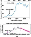 |
Fig. 1. Top panel: Inclination of the heliospheric current sheet computed in the potential-field source-surface approximation at Wilcox Solar Observatory during the progression of solar cycle 25, reported as a function of Carrington rotation number. Bottom panel: Solar cycle sunspot number progression for solar cycle 25 as a function of time (years) (source: NOAA/Space Weather Prediction Center website). The two different phases at which observations on February 22, 2021, and October 12, 2022, were carried out are highlighted by arrows in both panels. |
On October 12, 2022, white-light images of the solar corona in the wavelength band 580–640 nm were collected in a FoV from 1.76 R⊙ (the internal edge of the occulter) up to 3.10 R⊙. The uninterrupted observing sequence we analyzed started at 10:15:01 UT and ended at 20:16:44 UT, which resulted in a 10-hour dataset of 299 coronal brightness (B) images, equally spaced in time. The data were acquired with the total brightness Metis acquisition scheme (Antonucci et al. 2020b). This scheme provides high-cadence sequences of total-brightness (tB) images of the corona, which serve as a direct proxy for the plasma density. In this case, all the frames were acquired by switching the polarimeter acceptance angle by 90 degrees exactly halfway during the detector exposure time of 20 s. In order to improve the signal-to-noise ratio, six consecutive frames were averaged onboard (pixel by pixel), resulting in a single image delivered at a cadence of 121 s. Since the tB images are acquired with a binning of 2 × 2 pixels2, the size of the resulting images is 1024 × 1024 pixels2. At this distance of the spacecraft from the Sun, the spatial scale on the plane of the sky was ≃4400 km pixel−1, which corresponds to 0.006 R⊙ pixel−1. For comparison, the FoV of the observations carried out in February 2021 was in the range 3.1–5.7 R⊙ and the spatial resolution was ≃14 000 km pixel−1 (Table 1 summarizes the main observational characteristics of the observing runs of February 2021 and October 2022). The tB images were processed and calibrated to the mean solar disk brightness B⊙ following the procedure described in Romoli et al. (2021) and De Leo et al. (2023), as recently revised by Giordano et al. (2025).
Summary of the observational parameters and characteristics of the runs of February 22, 2021, and October 12, 2022.
A minimum background total brightness image was obtained by taking the minimum brightness in each pixel over the 299 acquired images, and then subtracted from each frame of the tB sequence. This procedure mainly removes the contributions from the F-corona through scattered photospheric light by dust grains, the instrumental scattered light, and the fraction of the K-corona globally produced by Thomson scattering by free electrons, which remains constant over the full observing run. In this way, the dynamic transient features of the K corona are highlighted (top panel of Fig. 2). In addition, to facilitate the identification and tracking of the density enhancements in the very active and highly structured solar corona of October 2022, a sequence of 298 running-difference tB images was obtained by subtracting the previous from the subsequent image (bottom panel of Fig. 2), following the procedure adopted in previous similar studies (e.g., Sheeley et al. 1997, 2009; Sanchez-Diaz et al. 2017). In the analysis performed in Paper I, this further processing step was not needed because of the relatively simple configuration of the corona and the low magnetic activity level at the epoch of the observations. These conditions allowed us to easily identify and characterize the density features in the first step of image processing, that is, to adopt the minimum background-subtracted sequence of images.
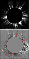 |
Fig. 2. Top panel: Metis tB image of the solar corona, captured on October 12, 2022, at 10:17:02 UT, after subtracting the minimum background image (field of view: 1.76–3.10 R⊙). Bottom panel: Running-difference image of the same frame as reported in the top panel. The three angular sectors are labeled A, B, and C. The associated movies of the full frames of the Metis observation sequences (background subtracted and running differences) are available online. |
3. Data analysis and results
In order to investigate the morphology and dynamics of the density enhancements detected in the solar corona, we analyzed the sequence of the running-difference tB images, focusing on the coronal sectors labeled A, B, and C in the bottom panel of Fig. 2.
The width of sectors A and B is about 60° and 40° in latitude and is centered at polar angles (measured counterclockwise from the north pole) PA = 320° and 120°, respectively. They were selected for analysis because they are both close in longitude to the tilted heliospheric current sheet, which lies relatively close to the plane of the sky, as shown in the two top panels of Fig. 3. The figure shows the Wilcox Solar Observatory (WSO) magnetic field computation results for Carrington rotation 2262 (more relevant for the east limb) and 2263 (closer in time to the October 12, 2022, observation and more relevant for the west limb). The bottom left panel of Fig. 3 shows the white-light LASCO C2 streamer map at r = 4.5 R⊙, constructed for the East limb observations. The bottom right panel reports the boundaries (separatrices) between open field regions at the source surface level r = 2.5 R⊙, derived by applying a potential-field source-surface (PFSS) extrapolation to the Global Oscillation Network Group (GONG; Harvey et al. 1996) map for CR 2263. In the synoptic map, Sectors A and B are located near longitudes 320° and 140°, respectively.
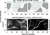 |
Fig. 3. Top panels: WSO magnetic field computations for Carrington rotations 2262 and 2263. The east and west limbs of the Sun are indicated by blue arrows. The dashed vertical line points out the Carrington longitude of Solar Orbiter with respect to the Earth, at the epoch of observations. Bottom left panel: LASCO C2 white-light coronal streamer structures at r = 4.5 R⊙ during CR 2263. Bottom right panel: Boundaries between open field regions at the source surface (r = 2.5 R⊙). The solid thick white line represents the source-surface neutral line (corresponding to the heliospheric current sheet), which separates holes of opposite polarity, and the thin gray lines mark the locations of pseudo-streamer plasma sheets, which separate holes with the same polarity. The values [90°, 0°, and –90°] of the latitudinal scale reported in the vertical axes match the polar angle values [360°, 270°, and 180°], respectively. |
The position of the heliospheric current sheet corresponds to the sites of two well-defined streamer structures, as resulting from the 3D MHD configuration obtained from the Predictive Science Inc. simulations, based on Helioseismic and Magnetic Imager (HMI; Schou et al. 2012; Scherrer et al. 2012) measurements on board the Solar Dynamics Observatory (SDO; Pesnell et al. 2012), and calculated considering the position of Solar Orbiter with respect to the Sun during the Metis observations of October 12, 2022 (see Fig. 4). This is the most favorable condition for the detection of density structures flowing outward from the Sun, as briefly mentioned in the Introduction.
 |
Fig. 4. Magnetic field lines traced on the plane of the sky on the basis of the 3D MHD model of the corona obtained from the Predictive Science Inc. simulations. The angular sectors A, B, and C are marked by thick white lines. |
Sector C, which ranges between the polar angle PA = 170° and 140°, was selected for comparison because its magnetic field configuration is fairly simple, with a neutral line almost parallel to the equator and without clear evidence of outflowing density features during the entire observational period.
Regions with highly complex and unstable magnetic configurations were neglected in the analysis because they are sources of energetic and explosive events that occurred during the observational run, therefore disrupting the ambient magnetic configuration and the morphology and dynamics of the regions (e.g., Romano et al. 2025, for the structure observed close to the north pole).
In regions A and B, a great number of features brighter-denser than the mean background coronal plasma is present (e.g., Fig. 5, concerning sector A). These structures appear to move outward from the Sun and rapidly evolve on a timescale even as short as the observation cadence. Some of the brightest features change morphology and brightness and some of them disappear, and in the meantime, new brightness enhancements appear. This highly dynamic behavior is typical of the phases of the solar cycle approaching or at solar maximum, as reported in several previous works (see e.g., Sanchez-Diaz et al. 2017; DeForest et al. 2018).
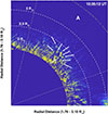 |
Fig. 5. Running-difference tB image of October 12, 2022, at 10:35:12 UT, corresponding to the northwest quadrant of the solar disk, where some of the brightest-densest features are indicated by white arrows. The two dashed radial white lines draw the angular borders of sector A. The white dashed arcs indicate heliocentric distances of 2.0, 2.5, and 3.0 R⊙. |
The radial and transverse sizes of the density features in sector A projected on the plane of the sky vary in the range from 45 to 65 ± 8 Mm (0.06–0.09 ± 0.01 R⊙) and 40–50 ± 8 Mm (0.06–0.07 ± 0.01 R⊙), respectively. These dimensions were determined by adopting the image segmentation and edge recognition procedures in MATLAB R2024a environment1 for a limited sample of the smallest and largest density structures in each frame and each selected sector. These procedures allowed us to interactively locate the pixels bounding each density feature we considered, to draw a region of interest (ROI), and to evaluate its size on the basis of the corresponding pixel spatial dimension. The uncertainty on the sizes of each feature was evaluated conservatively as twice the pixel resolution, that is, 0.012 R⊙ (8 Mm). The measured radial and transverse sizes in sector B range from about 30 to 75 ± 8 Mm (0.04–0.11 ± 0.01 R⊙) and 35 to 50 ± 8 Mm (0.05–0.07 ± 0.01 R⊙), respectively.
Compared with the same characteristics as the density structures observed on February 2021, whose radial and transverse dimensions are up to 500 Mm (0.70 R⊙) and 40 Mm (0.06 R⊙), respectively, they appear to be smaller. This agrees with the solar cycle modulation found by Alzate & Di Matteo (2025), who detected smaller structures during solar maximum.
For each coronal sector, we analyzed the Metis tB intensity along each of the 220 pixels in the radial direction, located at increasingly higher heliocentric distance in the range 1.76–3.10 R⊙, and at polar angles PA separated by 2°. The procedure was repeated for each of the 298 running-difference images of the observational sequence. The resulting time series of the tB intensity as a function of heliocentric distance in each radial direction were standardized, normalizing the data to zero mean and unit standard deviation in order to transform all values to a comparable scale.
In Fig. 6 the height-time maps of tB intensity are reported for each sector as a function of the observation time and heliocentric distance for some of the most representative radial directions we examined, in which the features are most evident and easily traceable. Each panel of Fig. 6 refers to different polar angles PA in one of the sectors A, B, and C, as reported at the top of each panel. They appear to be very different from the height-time maps obtained for the observations on February 22, 2021 (see Fig. 2 and Fig. 5 of Paper I), where few and isolated diagonal traces highlight persistent and well-defined bright features propagating outward. Conversely, in the present height-time maps, many diagonal traces, sometimes fragmented and discontinuous, underline fast-evolving brighter-denser structures, flowing in the FoV of the coronagraph in sectors A and B (see the left and middle panels of Fig. 6), due to the more complex and dynamically evolving magnetic configuration observed as the solar cycle progresses.
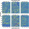 |
Fig. 6. Maps of the total brightness tB intensity as a function of time and heliocentric distance for sectors A (left panels), B (middle panels), and C (right panels) for some of the most representative radial directions considered in the analysis. Each time series of the total brightness tB is normalized to zero mean and unit standard deviation. The sector label is reported at the top of each corresponding panel, as well as the radial direction, expressed in terms of the polar angle (PA) value, measured counterclockwise from the north pole. The white and red arrows indicate outflowing and inflowing structures, respectively. The color gradient from blue to yellow progresses from low to high values of the total brightness. Yellow represents brighter structures. |
In sector A (left panels of Fig. 6) brighter-denser inhomogeneities flow outward at a polar angle PA = 316° and 346° (some of the brightest are indicated by white arrows) at an average speed of 240 ± 70 km s−1, as evaluated for a limited sample of more persistent and less-fragmented tracks with a clear and measurable slope. The corresponding uncertainty is the standard error of the mean. In the top left panel, a bright structure (indicated by a red arrow), appearing at 2.1 R⊙, flows inward, reaching the lower limit of the FoV at a speed of 200 ± 15 km s−1. In this case and in what follows, the speed reported for inflows is not an average value, but a value referring to individual tracks. The corresponding uncertainties were computed on the basis of the errors in the radial distance traveled, ΔH, (for which we assumed twice the pixel dimension, 0.012 R⊙) and the uncertainty on the corresponding time ΔT, for which we adopted (in a very conservative way) the cadence between frames in the sequence, that is, 121 sec. In the bottom left panel, density depletion inflows (see, e.g., Sheeley & Wang 2007; Wang & Hess 2018; Alzate et al. 2024) are observed as diagonal dark traces. The most evident trace, indicated by a red arrow, appears at about 2.4 R⊙ and moves inward at 90 ± 4 km s−1 down to 2.0 R⊙, where it fades away. It is interesting to note that the polar angle PA = 346° corresponds to the tip of the well-defined northwest streamer that is mapped in Fig. 4.
As in sector A, in the two panels relative to sector B (middle panels of Fig. 6 at polar angles PA= 106° and 110°), diagonal traces of many outflowing brighter-denser structures flowing at an average speed of 240 ± 70 km s−1 are evident. Inflowing depletions are observed at different heliocentric distances in the range from 2.4 to 3.0 R⊙. The dark traces indicate speeds ranging in a very wide interval from 100 ± 9 km s−1 down to 35 ± 1 km s−1. Some of them, especially those in the middle-bottom panel of Fig. 6 at PA = 110°, show a final deceleration, as revealed by the upward curve of the tracks, before they fade away. This agrees with the hypothesis mentioned above that inflows are triggered when streamer loops pinch off (Wang 2024). According to this hypothesis, the collapsing loop cusps first accelerate in response to the magnetic tension and then decelerate as they approach their final equilibrium position. The polar angle PA = 110° corresponds to the site at the borders of the southeast streamer, evident in the 3D MHD model of the coronal magnetic field (Fig. 4). Conversely, the panels referring to sector C (right panels of Fig. 6) reflect quite different magnetic activity conditions. Sporadic outflowing density enhancements and inflows are visible at the two latitudes reported in the figure.
The second step of our analysis consisted of the search for any potential periodicities characterizing the release of the density features observed in sectors A and B (sector C was also investigated for comparison), following what was found in Paper I. A spectral analysis of each time series was performed pixel-by-pixel along the radial directions, 2° apart, inside each sector in the entire FoV of the coronagraph. We adopted the Lomb-Scargle algorithm (Scargle 1982) for unequally spaced data due to the presence of gaps in the final processed observational sequence, which were introduced by the removal of a limited number of corrupted images that were due to debris passing in front of the telescope aperture during the observations.
Figure 7 shows, as an example, the power spectra obtained for PA = 316° and 346° (sector A), 106° and 110° (sector B) and 158° and 152° (sector C) at three different heliocentric distances (1.80, 2.40, and 3.0 R⊙) along each radial direction. The PAs reported are the same as in Fig. 6. All power spectra, regardless of the sector and the radial direction we examined, show significant power peaks (higher than at least the 95% confidence level) at different frequencies within a band extending from about 2.4 to 3.6 mHz. These fluctuations are present in all the sectors we examined, regardless of their magnetic configuration, level of activity, and density enhancements detected in the previous step of the analysis.
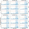 |
Fig. 7. Lomb-Scargle periodograms, each of them normalized to its maximum power, for sectors A (left panels), B (middle panels), and C (right panels) for the same radial directions as considered in Fig. 6. The sector labels are reported at the top of each corresponding panel, as well as the radial direction, expressed in polar angle (PA) value. The corresponding heliocentric distances of the periodograms (1.8, 2.4, and 3.0 R⊙) are shown at the right side of each panel. The horizontal lines report confidence levels of 95% (in yellow) and 99% (in red). The light blue shaded area in each panel highlights the frequency band 2.4–3.6 mHz, where a strong concentration of power, higher than at least the 95% confidence level, is persistently present at different frequencies. |
The results we obtained agree with the work recently published by Andretta et al. (2025), based on observations carried out on October 8, 2022, very close in time to the observations presented here. They suggested that density fluctuations with a period of about 5 minutes (3.3 mHz) are ubiquitously present in the corona from 1.76 R⊙ to 3.10 R⊙, that is, in the entire radial FoV of the coronagraph and in a wide range of latitudes.
To improve the signal-to-noise ratio and reveal any possible recurrence in the release of the enhanced density features hidden by the predominant periodicities in the frequency band 2.4–3.6 mHz, we divided each sector into smaller subsectors, 5°, 10°, and 20° wide. Specifically, sector A, 60° wide, was divided into 12, 6, and 3 subsectors, sector B, 40° wide, was divided into 8, 4, and 2 subsectors, and sector C, 30° wide, was divided into 6 and 3 subsectors. Table 2 presents the subsectors we identified, each labeled with a unique name. For each subsector, the table provides the corresponding angular extent, measured in terms of the PA boundaries.
Angular range of the subsectors of sectors A, B, and C.
The procedure was iteratively applied to all the images of the temporal sequence. Ultimately, we obtained 220 (the number of pixels along the radial distance) time series of tB intensity in each subsector; for each series, we computed the Lomb-Scargle periodogram.
Fig. 8 shows a synoptic view of the periodicities found at 1.8 R⊙ for each subsector considered, provided they have a confidence level greater than or equal to 95%. First of all, we note that the periodicities present in the frequency band 2.4–3.6 mHz in the periodograms reported in Fig. 7 fall below the minimum confidence threshold fixed at 95% probably due to the averaging effect over the latitude of a signal that is not spatially coherent. As appears to be evident in Fig. 8, two periodicities, at 13 min and 42 min, satisfy the condition fixed on the confidence level in specific subsectors (see Table 2 for the correspondence between the custom names and angular range). The 13 min periodicity is present in subsectors A10, A11, A12 (5° wide), A18, A19 (10° wide), and A21 (20° wide) of sector A (see the top panel of Fig. 8), and also in all the subsectors of sector B (see middle panel) and C (see bottom panel). The 42 min periodicity is present in subsectors A7, A8 (5° wide), A16 (10° wide), and A20 (20° wide) of sector A, where this periodicity alone has a confidence level of at least of 95%. All periodograms referring to the subsectors of sector A outside this area show no significant peaks above the established minimum confidence threshold. It is worth highlighting that all the subsectors of sector A reported above are located inside an angular region within the PA range [320°–310°], where as a consequence we can argue that the signal of the 42 min periodicity is presumably confined. The 42 min periodicity is also present in subsectors B4, B6, B7, B8 (5° wide), B10, B11, B12 (10° wide), and B14 (20° wide) of sector B, where the 13 min periodicity is also present. Outside this region (i.e., in the PA range [140°–120°]), the 13 min periodicity is the only peak in all the periodograms with a power above at least the minimum confidence threshold. For the same reason as explained for sector A, we can conclude that in sector B, the 42 min periodicity is presumably confined approximately in the PA range [120°–100°]. In none of the subsectors of sector C is the 42 min periodicity present.
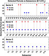 |
Fig. 8. Synoptic view of the results of the spectral analysis performed for each subsector of sectors A (top panel), B (middle panel), and C (bottom panel) at 1.8 R⊙. The subsectors are labeled according to Table 2, and the reported periodicities are those with a confidence level of at least 95%. As indicated in each panel, the blue and red bullets refer to the 13 min and 42 min periodicities, respectively. |
Fig. 9 shows, as an example, the periodograms of subsectors A16 of sector A, B14 of sector B, and C8 of sector C (see Table 2), all computed at 1.8 R⊙. The subsectors we selected were chosen to show the power spectra where the signal has its maximum power. The periodogram of subsector A16 (see Table 2) of sector A (see Fig. 9, top panel) is dominated, well above the 99% confidence level, by a peak corresponding to the periodicity of 42 min, while the periodicity of about 13 min is well below the 95% confidence level and barely visible. The periodogram of subsector B14 (see Table 2) of sector B (see Fig. 9, middle panel) shows two peaks above the 99% confidence level, corresponding to periodicities of 42 min and 13 min. The periodogram reported in the bottom panel of Fig. 9 for subsector C8 (see Table 2) of sector C is dominated by a peak corresponding to the 13 min periodicity well above the 99% confidence level, and no other peaks are distinguishable above the noise. It is a very representative example of the periodograms obtained for all subsectors of sector C.
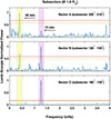 |
Fig. 9. Lomb-Scargle periodograms, each of them normalized to its maximum power, for subsectors of sectors A (top panel), B (middle panel), and C (bottom panel), computed at a radial distance of 1.8 R⊙. The latitudinal range of each subsector is indicated in each panel. The peaks at 42 min and 13 min are indicated by arrows and highlighted by a light yellow and a light magenta shaded area, respectively. The 95% and 99% confidence levels are reported as solid yellow and red lines, respectively. |
The persistence of the 13 min periodicity with a power about five times the 99% confidence level in all the periodograms of the subsectors of sector C, relatively quiet and with only sporadic evidence of outflowing density features, raises some doubts about its origin. In Appendix A.1 we describe the analysis in detail that we carried out to investigate the possibility that it is a spurious component caused by instrumental effects. The investigation was mainly based on a test carried out on the Metis ground reference model. The results we obtained allow us to conclude that the 13 min periodicity is a spurious modulation of instrumental origin.
Before we proceeded, we filtered out the original time series by removing this periodicity from all subsectors where it was present. The amplitudes and phases are those resulting from the least-squares fit provided by the Lomb-Scargle procedure. Then, we again computed the Lomb-Scargle periodograms for each subsector as a function of the radial distance. Figure 10 reports the periodograms of the filtered-out time series obtained for four different radial distances 1.8, 2.0, 2.2, and 2.4 R⊙ in the same regions as reported in Fig. 9. The most prominent power in the subsectors (indicated at the top of each panel) of sectors A (left panels) and B (middle panels) peaks at about 0.40 mHz (42 min) and remains significant from the inner limit of the FoV up to 2.2 R⊙, with a power higher than or equal to the 99% confidence level. At 2.4 R⊙ the corresponding signal weakens, fading into the noise. In the periodogram of sector C (right panels), the filtering-out procedure leaves only noisy spectra at all the radial distances we considered.
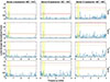 |
Fig. 10. Lomb-Scargle periodograms, each of them normalized to its maximum power, for subsectors of sector A (left panels), B (middle panels), and C (right panels) after the filtering-out of the instrumental periodicity of 13 min, computed at radial distances of 1.8, 2.0, 2.2, and 2.4 R⊙ as reported at the right side of each panel. The peaks at 42 min are highlighted by a light yellow shaded area. The 95% and 99% confidence levels are reported as solid yellow and red lines, respectively. |
In order to ascertain the nature of the 42 min periodicity and to be able to rule out the possibility that it is an artifact caused by instrumental effects or data-sampling irregularities, we carried out a further investigation. We refer to Appendix A.2 for a detailed description of the analysis we conducted. The results obtained fully agree, converge to exclude an instrumental origin of the 42 min periodicity, and support its solar nature.
It is now essential to examine the cause of this periodicity in particular areas of the corona and to explore any potential correspondence with specific magnetic structures, such as streamers and pseudo-streamers, along with their substructures, including boundaries, cusps, and stalks, which may play a role in the release of the observed density features. Fig. 11 shows the tB coronal emission in the two northwest and southeast quadrants of the solar corona on October 12, 2022, as detected by Metis at 10:35:12 UT. The two latitudinal ranges [320°–310°] (subsector A16 of sector A, left panel) and [120°–100°] (subsector B14 of sector B, right panel), corresponding to the regions where the 42 min periodicity was detected with a higher level of significance, are indicated. The correspondence between the subsectors and the outflowing density features is clear: the highest concentration of them is just within the specific regions of interest. Then, we can relate the 42 min periodicity to the release of the density structures that flow out of the solar corona, according to some mechanism that controls their ejection. Furthemore, in Fig. 4, the two subsectors of interest can be correlated to the borders of the two well-defined streamers in sectors A and B, characterizing the magnetic configuration in the epoch of the observation and corresponding to the position of the heliospheric current sheet.
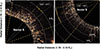 |
Fig. 11. Running-difference tB image of October 12, 2022, at 10:35:12 UT (the same as in Fig. 5) corresponding to the northwest (left panel) and southeast (right panel) quadrants of the solar disk. The two solid dashed radial yellow lines draw the angular borders of sectors A and B, and the dashed white arcs indicate heliocentric distances of 2.0, 2.5, and 3.0 R⊙ in both panels. Subsector A16 ([320° − 310°] of sector A and subsector B14 ([120°–100°] of sector B are also reported in each panel. |
4. Discussion
During the 10-hour observation of the Metis coronagraph on October 12, 2022, when Solar Orbiter was transiting at perihelion at 0.29 au, the solar corona was quite structured, with rapidly evolving regions and sources of energetic and explosive events, such as the eruption of the polar crown prominence at the northeast limb studied by Romano et al. (2025). In addition, the coronal plasma at a heliocentric distance of about 3 R⊙ was characterized by a fully developed turbulence resulting from the evolution of a diffuse background of density fluctuations, as shown by the investigation of Telloni et al. (2024), based on the same set of data.
Notwithstanding the complexity of the coronal magnetic field, two sections of the streamer belt, about 60° and 40° wide in latitude, running almost parallel to and near the southeast and northwest solar limbs, were intercepted along the line of sight of the Metis coronagraph in relatively quiet coronal regions. The high tilt of the two streamer belt segments, observed to be almost aligned with the limb, is due to the presence of a warped belt, caused by the quadrupolar component of the global magnetic field characterizing the ascending phase of the solar cycle. These quiet coronal regions were explored in the heliocentric distance range from 1.76 to 3.10 R⊙ at high temporal (2 min) and spatial (4 400 km pixel−1) resolution, by analyzing the white-light total brightness, which is considered a direct proxy for the plasma density.
Many and frequent small-scale density features with radial size ranging from 30 to 75 ± 8 Mm (0.04–0.10 ± 0.01 R⊙) were observed to propagate outward at a speed of about 240 ±70 km s−1 on average (Fig. 6) in two selected sectors named A and B. The outflowing coronal transients appeared to be numerous, at least up to 2.4 R⊙, with a higher concentration in the range 2.0–2.4 R⊙ (see Fig. 6). Farther out, the majority of these structures progressively faded. The outflows were intermingled with downflows, clearly identifiable as dark lanes in Fig. 6, which were observed to mainly originate in the range of heliocentric distances 2.1–3.0 R⊙ at the interface between open and closed magnetic field lines at the borders of the streamers, up to regions close to the streamer cusp. The outflows throughout sectors A and B and inflows close to the borders of the two streamer segments might be interpreted in terms of frequent reconnection events between open and closed field lines occurring in the inner-medium corona, in analogy with the considerations of Wang & Hess (2018) for the top region of well-developed helmet streamers, and in the case of inflows, of probable pinch-off of the streamer loops. The density structures observed in the 3-hour interval of the Metis solar minimum observation in February 2021 (Paper I) were elongated in the radial direction (about 500 Mm, 0.7 R⊙ radial size and 40 Mm, 0.06 R⊙ transverse size) and crossed the full field of view with a speed of 240 km s−1, which is on the same order as that observed for the density transients detected in the present work. In both cases, the speed of the transients exceeded the outflow speed of the ambient solar wind, determined by previous Metis observations during the solar minimum of cycle 24 (Romoli et al. 2021; Antonucci et al. 2023).
At a given helio-latitude, the frequency analysis of the temporal evolution of the coronal total brightness tB observed on October 12, 2022, does not highlight any significant periodicity in the occurrence of the outflowing small-scale density structures. It instead reveals density fluctuations in the frequency range 2.4–3.6 mHz throughout the corona. These fluctuations are present in all the sectors we examined, regardless of their magnetic configuration, level of activity, and density enhancements. This lack of recurrence apparently differs from the behavior of the transients detected at the solar minimum in February 2021, characterized by a clear periodicity of about 80 min (Paper I). In the latter case, however, the streamer belt was almost equatorial, so that the line of sight ran parallel to the almost equatorial streamer belt (and associated heliospheric current sheet), which was observed edge-on. Thus, at that time, the Metis coronagraph acquired the emission, integrated along the line of sight, of propagating structures that might have originated at a given latitude, but at different longitudes.
This possibility is supported by the fact that when we integrated the coronal emission over relatively narrow subsectors and analyzed it as a function of the radial distance, a well-defined periodicity was retrieved in specific regions, while the signal inside the frequency band 2.4–3.6 mHz fell below the minimum confidence threshold fixed at 95%, or even faded into the noise, probably due to the averaging effect over the latitude of a signal that is not spatially coherent. Observed in the inner corona and along a tilted streamer belt, the density enhancements recur with a period of 42 min, which is much shorter than the 80 min periodicity observed in the medium-outer corona at heights above 3 R⊙ during solar minimum (Paper I). Periodicities below 80 min were already reported by DeForest et al. (2018) during a phase of high solar activity in 2014. In this case, coronal density features detected above 5 R⊙ were released at a cadence of 20 min during a STEREO-COR2 observational campaign performed with a temporal resolution of 5 min. A pattern of intermittent magnetic reconnection, similar to the results obtained in this study, was observed just above helmet streamers, along a highly tilted neutral sheet during solar maximum of cycle 24, when quasi-periodic bursts of activity with simultaneous release of coronal blobs at all latitudes were detected by Sanchez-Diaz et al. (2017). In this case, the typical radial size of the coronal transients was much larger, 12 R⊙ on average, and was released with a cadence of 19.5 h. In a shorter observing interval lasting 10 hours, the high temporal and spatial resolution observations of the Metis coronagraph suggest a similar recurrent magnetic reconnection process involving a specific latitude range of the tilted streamer belt. This process, however, acts on a much smaller scale, resulting in the release into the ambient solar wind of small-scale plasmoids at a much higher frequency. In addition, coronal blobs such as those observed by Sanchez-Diaz et al. (2017) are typically emitted at the apex of streamers, for instance, either by streamer loop pinch-off to form a flux rope (Wang 2012; Wang & Hess 2018), or by reconnection triggered via a tearing mode at the heliospheric current sheet forming at the tip of streamers (Réville et al. 2020).
As observed in the maps of Fig. 6, the density structures were more frequently observed between 2.0 and 2.4 R⊙. However, the coronal region in which these structures could have been observed extends to 1.76 R⊙. Therefore, they might be released even below this height. The differentiation in plasmoids detected in the lower layers of the corona, from below 1.76 R⊙ up to about 2 R⊙, and the more numerous plasmoids detected at 2.0–2.4 R⊙ is based on the analysis performed at high spatial resolution in latitude. When the analysis was performed considering the coronal emission integrated over the latitude range of specific subsectors, the periodicity of 42 min in the release of plasmoids was clearly observed up to about 2.4 R⊙ at least. Under the hypothesis that we detected two different classes of plasmoids that originate in the range 1.76–2.0 R⊙ and between 2.0 and 2.4 R⊙, the height distribution of the periodic transients observed with Metis shows some similarities with the results obtained by Alzate et al. (2024). On the basis of the Extreme Ultraviolet Imager (EUI; Rochus et al. 2020) on board Solar Orbiter and the COR1 and COR2 coronagraphs of the STEREO mission, these authors identified two classes of density structures released in the inner-medium corona, the slow transients formed at about 1.6 R⊙ (thus propagating in the region covered by the Metis FoV) and flowing around the streamer boundaries, and faster structures, predominantly originating at about 3 R⊙ and often propagating within the streamer boundaries. However, these observations were made in a solar minimum phase, and the plasma release occurred at a cadence 98–128 min, with an initial speed of 16–88 km s−1, and acceleration at higher heliocentric distances up to about 200 km s−1 at 7.5 R⊙.
The enhanced density structures observed with Metis at lower heights originate in a region where the streamer magnetic field lines are predominantly closed, and the heliospheric current sheet between open lines of opposite polarities is not yet formed. In this case, the Metis density features might be produced by interchange reconnection at pseudo-streamer cusp located below ∼1.6–1.7 R⊙. In the bottom right panel of Fig. 3, the presence of pseudo-streamers in the magnetic configuration corresponding to the CR 2263 is indicated by the gray lines, branching off the solid thick white lines marking the heliospheric current sheet and separating coronal holes with the same polarity. Pseudo-streamers are very common near solar maximum because during this phase of the solar cycle, many small fragmentary coronal holes with the same polarity located near each other, as well as large holes with irregular shapes, characterize the solar magnetic configuration. This is shown in Fig. 12, which displays the map of open field regions derived by the GONG photospheric magnetic field for CR 2263. We note that the most affected longitudes are ∼150° in the south and 320°–360° in the north, approximately corresponding to the overlying sectors A and B.
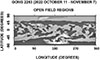 |
Fig. 12. GONG map of open field regions at the Sun’s surface derived for CR 2263. The values [90°, 45°, 0°, -45°, and -90°] of the latitudinal scale reported in the vertical axis match the polar angle values [360°, 315°, 270°, 225°, and 180°], respectively. The background polarities are indicated in dark gray when they are negative and light gray when they are positive. |
On the other hand, the reconnection that causes the structures that form higher up at 2.0–2.4 R⊙ are expected to take place closer to the heliospheric current sheet as the result of interchange reconnection at the helmet streamer cusps, and it might be related to processes characterizing the streamer cusp itself. We also note that in the streamers of sectors A and B, one of the boundaries is better observed since it lies closer to the plane of the sky because of the high tilt of the streamer structures. Hence, this supports the interpretation that relates the 42 min modulation of the plasma structures flowing in the lower coronal layers to plasma-release processes in regions close to or at the streamer boundaries.
The most relevant result we obtained is that the magnetic reconnection processes that cause the small-scale plasmoid release are activated in areas encompassing 10°–20° wide subsectors, corresponding to a spatial scale of about 0.2–0.3 R⊙, where density structures are ejected according to some periodic clock. That is, the response of the corona appears periodic in time and locally coherent, but not uniform over the entire sectors.
Based on the preferential occurrence of plasma-release processes at the streamer boundaries as well as close to the streamer cusps, we formulate the hypothesis that the energy release and consequent ejection of density structures is modulated by convection patterns on the solar surface. However, the observed recurrence time cannot be directly associated with the typical timescales of solar surface convective motions: supergranulation, mesogranulation, or granulation, on the order of 1 day, about 2 hours, and in the range of about 6–16 min, respectively. Moreover, the scale of the area involved in the periodic release of density structures exceeds the supergranular dimensions by one order of magnitude. On the other hand, we cannot exclude that some of the supergranulation features might be related to the periodic release of the small-scale coronal transients. The size of the transient density structures, 30-75 Mm (0.04–0.10 R⊙), is compatible with the supergranulation scale, within 20–55 Mm (0.03–0.08 R⊙). In addition, supergranular boundaries are known to be the site of intense magnetic flux tubes, which are magnetic field lines that are swept up by the motions in the cells toward the cell boundaries. Magnetic elements of mixed polarities, with lifetimes of about 30 min, can also be present within a supergranular cell. It is interesting to note that supersonic flows have been observed at the boundaries between granules and supergranules and are expected to produce shocks (Bellot Rubio 2009). Supergranular junctions can also be the site of vortices: when two merging flux tubes are trapped inside a vortex, at the centers of the flux tubes, the magnetic field is intensified in a 30 min time interval (Chian et al. 2023). The emergence of intense magnetic flux tubes likely creates the conditions for the interchange reconnection of open and closed field lines in the inner coronal layers of the streamer belt. Shocks, and possibly vortices, at the supergranular boundaries might play an important role in triggering the interchange reconnection process with release of periodic density enhancements into the ambient solar wind, as observed during the ascending phase of solar activity.
5. Conclusions
During the 10-hour observations performed in the heliocentric distance range 1.76–3.10 R⊙ of the solar corona, small-scale density structures (30–75 Mm, 0.04–0.10 R⊙, in size) were released along segments with a length of about 0.2–0.3 R⊙ of the warped streamer belt. This is characteristic of the ascending phase of the solar cycle. They propagated outward in the corona at about 240 km s−1 on average. They were well observed in their outward propagation above the limb and appeared to be more numerous from 2.0 R⊙ out to 2.4 R⊙.
Metis density features located farther from the heliospheric current sheet might be produced by reconnection at pseudo-streamer cusps located at lower heights, whereas the density features located close to the heliospheric current sheet might be the result of interchange magnetic reconnection at the helmet streamer cusps at greater heights. The high tilt of the streamer belt relative to the solar equatorial plane allowed us to conclude that these density features are ejected according to a periodic trigger, acting in a latitudinal range of about 10°–20°. That is, the response of the corona is periodic in time as well as coherent in space over specific narrow areas, considering that the periodicity of 42 min was obtained only by integrating the coronal emission over a 10°–20° range of latitudes and in correspondence of specific regions, where the density structures are mainly concentrated.
The ejection of the small coronal transients, which are predominantly released in the low corona, can reasonably be ascribed to a process of magnetic reconnection caused by the interchange of open and closed magnetic field lines that is triggered in specific locations along the streamer with a 42 min periodicity. Although the considerations we presented in the discussion section cannot be considered as conclusive, the suggestion is plausible that the driver of the quasi-periodic release of density structures in the solar corona and solar wind is related to the convective motions on the solar surface and to the emergence of flux tubes, as well as to the propagation of shocks at the boundaries of the convection cells.
Data availability
Movies associated with Figs. 2 are available at https://www.aanda.org
Acknowledgments
Solar Orbiter is a space mission of international collaboration between ESA and NASA, operated by ESA. Metis has been built and is operated with funding from the Italian Space Agency (ASI), under contracts to the National Institute of Astrophysics (INAF) and industrial partners. Metis has been built with hardware contributions from Germany (Bundesministerium für Wirtschaft und Energie through DLR), from the Czech Republic (PRODEX) and from ESA.
References
- Alzate, N., & Di Matteo, S. 2025, ArXiv e-prints [arXiv:2509.12009] [Google Scholar]
- Alzate, N., Di Matteo, S., Morgan, H., Viall, N., & Vourlidas, A. 2024, ApJ, 973, 130 [Google Scholar]
- Andretta, V., Abbo, L., Jerse, G., et al. 2025, A&A, 701, A199 [NASA ADS] [CrossRef] [EDP Sciences] [Google Scholar]
- Antiochos, S. K., Linker, J. A., Lionello, R., et al. 2012, Space Sci. Rev., 172, 169 [Google Scholar]
- Antonucci, E. 2006, Space Sci. Rev., 124, 35 [Google Scholar]
- Antonucci, E., Harra, L., Susino, R., & Telloni, D. 2020a, Space Sci. Rev., 216, 117 [CrossRef] [Google Scholar]
- Antonucci, E., Romoli, M., Andretta, V., et al. 2020b, A&A, 642, A10 [NASA ADS] [CrossRef] [EDP Sciences] [Google Scholar]
- Antonucci, E., Downs, C., Capuano, G. E., et al. 2023, Phys. Plasmas, 30, 022905 [Google Scholar]
- Bellot Rubio, L. R. 2009, ApJ, 700, 284 [NASA ADS] [CrossRef] [Google Scholar]
- Brueckner, G. E., Howard, R. A., Koomen, M. J., et al. 1995, Sol. Phys., 162, 357 [NASA ADS] [CrossRef] [Google Scholar]
- Chian, A. C. L., Rempel, E. L., Silva, S. S. A., Bellot Rubio, L., & Gošić, M. 2023, MNRAS, 518, 4930 [Google Scholar]
- Cranmer, S. R., Gibson, S. E., & Riley, P. 2017, Space Sci. Rev., 212, 1345 [Google Scholar]
- De Leo, Y., Burtovoi, A., Teriaca, L., et al. 2023, A&A, 676, A45 [NASA ADS] [CrossRef] [EDP Sciences] [Google Scholar]
- DeForest, C. E., Howard, R. A., Velli, M., Viall, N., & Vourlidas, A. 2018, ApJ, 862, 18 [Google Scholar]
- Di Matteo, S., Viall, N. M., Kepko, L., et al. 2019, JGRA, 124, 837 [Google Scholar]
- Domingo, V., Fleck, B., & Poland, A. I. 1995, Sol. Phys., 162, 1 [Google Scholar]
- Fineschi, S., Naletto, G., Romoli, M., et al. 2020, Exp. Astron., 49, 239 [Google Scholar]
- Giordano, S., Spadaro, D., Susino, R., et al. 2025, A&A, 701, A56 [NASA ADS] [CrossRef] [EDP Sciences] [Google Scholar]
- Harvey, J. W., Hill, F., Hubbard, R. P., et al. 1996, Science, 272, 1284 [Google Scholar]
- Howard, R. A., Moses, J. D., Vourlidas, A., et al. 2008, Space Sci. Rev., 136, 67 [NASA ADS] [CrossRef] [Google Scholar]
- Howard, R. A., Vourlidas, A., & Stenborg, G. 2023, Front. Astron. Space Sci., 10, 1264226 [NASA ADS] [CrossRef] [Google Scholar]
- Hyder, C. L., & Lites, B. W. 1970, Sol. Phys., 14, 147 [Google Scholar]
- Jones, S. I., & Davila, J. M. 2009, ApJ, 701, 1906 [NASA ADS] [CrossRef] [Google Scholar]
- Kaiser, M. L. 2005, Adv. Space Res., 36, 1483 [NASA ADS] [CrossRef] [Google Scholar]
- Kepko, L., Viall, N. M., Antiochos, S. K., et al. 2016, Geophys. Res. Lett., 43, 4089 [NASA ADS] [CrossRef] [Google Scholar]
- Kepko, L., Viall, N. M., & DiMatteo, S. 2024, J. Geophys. Res. (Space Phys.), 129, e2023JA031403 [NASA ADS] [CrossRef] [Google Scholar]
- Kohl, J. L., Esser, R., Gardner, L. D., et al. 1995, Sol. Phys., 162, 313 [Google Scholar]
- Müller, D., St. Cyr, O. C., Zouganelis, I., et al. 2020, A&A, 642, A1 [Google Scholar]
- Pesnell, W. D., Thompson, B. J., & Chamberlin, P. C. 2012, Sol. Phys., 275, 3 [Google Scholar]
- Pylaev, O. S., Zaqarashvili, T. V., Brazhenko, A. I., et al. 2017, A&A, 601, A42 [NASA ADS] [CrossRef] [EDP Sciences] [Google Scholar]
- Réville, V., Velli, M., Rouillard, A. P., et al. 2020, ApJ, 895, L20 [Google Scholar]
- Rochus, P., Auchère, F., Berghmans, D., et al. 2020, A&A, 642, A8 [NASA ADS] [CrossRef] [EDP Sciences] [Google Scholar]
- Romano, P., Wyper, P., Andretta, V., et al. 2025, ApJ, 982, 142 [Google Scholar]
- Romoli, M., Antonucci, E., Andretta, V., et al. 2021, A&A, 656, A32 [NASA ADS] [CrossRef] [EDP Sciences] [Google Scholar]
- Sanchez-Diaz, E., Rouillard, A. P., Davies, J. A., et al. 2017, ApJ, 851, 32 [Google Scholar]
- Scargle, J. D. 1982, ApJ, 263, 835 [Google Scholar]
- Scherrer, P. H., Schou, J., Bush, R. I., et al. 2012, Sol. Phys., 275, 207 [Google Scholar]
- Schou, J., Scherrer, P. H., Bush, R. I., et al. 2012, Sol. Phys., 275, 229 [Google Scholar]
- Sheeley, N. R., Jr, & Wang, Y. M. 2007, ApJ, 655, 1142 [NASA ADS] [CrossRef] [Google Scholar]
- Sheeley, N. R., Wang, Y. M., Hawley, S. H., et al. 1997, ApJ, 484, 472 [Google Scholar]
- Sheeley, N. R. J., Lee, D. D. H., Casto, K. P., Wang, Y. M., & Rich, N. B. 2009, ApJ, 694, 1471 [NASA ADS] [CrossRef] [Google Scholar]
- Telloni, D., Sorriso-Valvo, L., Zank, G. P., et al. 2024, ApJ, 973, L48 [Google Scholar]
- Thompson, W. T., Davila, J. M., Fisher, R. R., et al. 2003, SPIE Conf. Ser., 4853, 1 [Google Scholar]
- Uslenghi, M., Andretta, V., Teriaca, L., et al. 2024, SPIE Conf. Ser., 13103, 1310324 [Google Scholar]
- Ventura, R., Antonucci, E., Downs, C., et al. 2023, A&A, 675, A170 [NASA ADS] [CrossRef] [EDP Sciences] [Google Scholar]
- Viall, N. M., & Vourlidas, A. 2015, ApJ, 807, 176 [Google Scholar]
- Viall, N. M., DeForest, C. E., & Kepko, L. 2021, Front. Astron. Space Sci., 8, 139 [NASA ADS] [CrossRef] [Google Scholar]
- Wang, Y. M. 2012, Space Sci. Rev., 172, 123 [NASA ADS] [CrossRef] [Google Scholar]
- Wang, Y. M. 2024, Sol. Phys., 299, 54 [NASA ADS] [CrossRef] [Google Scholar]
- Wang, Y. M., & Hess, P. 2018, ApJ, 859, 135 [NASA ADS] [CrossRef] [Google Scholar]
- Wang, Y. M., Sheeley, N. R., Socker, D. G., Howard, R. A., & Rich, N. B. 2000, J. Geophys. Res., 105, 25133 [NASA ADS] [CrossRef] [Google Scholar]
- Withbroe, G. L., Kohl, J. L., Weiser, H., & Munro, R. H. 1982, Space Sci. Rev., 33, 17 [Google Scholar]
Appendix A: Origin of the 13-min and 42-min periodicities
A.1. The 13-min periodicity
In order to ascertain the nature of the 13-min periodicity found in the periodograms of many of the subsectors of Sector A and B, and in all the subsectors of Sector C (see as an example Fig. 9), we carried out a test based on the Metis Ground Reference Model, which is a hardware replica of the Metis instrument, used as a test bench to replicate the performance of the detectors and characterize electronic noise affecting the entire sensor (including the dark areas), such as specific periodic signal modulations observed in the flight signal intensity. We acquired a set of 299 dark images with the same exposure time (Detector Integration Time, DIT, 20 sec), the number of frames averaged, pixel-by-pixel, in order to obtain the final images (Number of Detector Integrations, NDIT, 6) and cadence (121 sec) parameters as in the onflight Metis sequence here analyzed, in a box of size 499 x 2018 pixels2, located in the top part of the detector (full detector size 2048x 2048 pixels2). Spectral analysis of the time series obtained by averaging the signal within the box at each time instance was carried out by applying the Lomb-Scargle procedure. The periodogram obtained is reported in Fig. A.1, where the 13-min periodicity is the only peak clearly evident above the noise. Then, we can conclude that a spurious periodicity of instrumental origin contributes to the 13-min periodicity. Previous studies on the instrumental effects of the Solar Orbiter/Metis detectors, electronics and acquisition modes have been performed by Uslenghi et al. (2024) and Andretta et al. (2025), who found that different instrumental frequencies are generated by different triplets of DIT, NDIT and cadence values of the observations. Changing the acquisition parameters resulted in frequency variations, or even absence of spurious frequencies, suggesting a correlation with the timing control exerted by the Metis Processing and Power Unit (MPPU) on the detector.
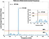 |
Fig. A.1. Lomb-Scargle periodogram resulting from the Reference Model test. The vertical black line indicates the frequency value 0.4 mHz, corresponding a period of 42 min. The inset shows the periodogram in a zoomed-in x scale in the range (0 - 1 mHz). |
A.2. The 42-min periodicity
The origin of the 42-min periodicity found in the periodograms of two specific regions inside the Sector A and Sector B has been also, accurately investigated. Since a limited number of corrupted images have been removed from the temporal sequence, as specified in Section 3.1, we computed the spectral window of the temporal sampling searching for any artifacts and/or aliasing effects that could be induced in the frequency domain by the presence of gaps in the data. Figure A.2 and its inset with a zoomed-in x-scale, show the results. The spectral window presents a simple uniform behaviour with low-amplitude sidelobes, rapidly decreasing as moving away from the main lobe, and is free from spurious peaks generated by the gaps present in the temporal sampling. Moreover, reconsidering the result of the Metis Reference Model analysis conducted for the 13-min periodicity we note that the periodogram of the temporal series (see Fig. A.1 ) does not show any other significant peak (in particular in the frequency range corresponding to the 42-min periodicity) apart from the very strong one at 13 min. The periodicities of the thermal system have also been examined, as they could in principle produce signal variations, but they are not compatible with this period. All the results obtained confirm that the 42-min periodicity is neither instrumental in origin nor an artifact resulting from data gaps.
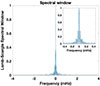 |
Fig. A.2. Spectral window of the unequally spaced data set analyzed. The inset shows the spectral window with a zoomed-in x-scale |
All Tables
Summary of the observational parameters and characteristics of the runs of February 22, 2021, and October 12, 2022.
All Figures
|
Fig. 1. Top panel: Inclination of the heliospheric current sheet computed in the potential-field source-surface approximation at Wilcox Solar Observatory during the progression of solar cycle 25, reported as a function of Carrington rotation number. Bottom panel: Solar cycle sunspot number progression for solar cycle 25 as a function of time (years) (source: NOAA/Space Weather Prediction Center website). The two different phases at which observations on February 22, 2021, and October 12, 2022, were carried out are highlighted by arrows in both panels. |
| In the text | |
|
Fig. 2. Top panel: Metis tB image of the solar corona, captured on October 12, 2022, at 10:17:02 UT, after subtracting the minimum background image (field of view: 1.76–3.10 R⊙). Bottom panel: Running-difference image of the same frame as reported in the top panel. The three angular sectors are labeled A, B, and C. The associated movies of the full frames of the Metis observation sequences (background subtracted and running differences) are available online. |
| In the text | |
|
Fig. 3. Top panels: WSO magnetic field computations for Carrington rotations 2262 and 2263. The east and west limbs of the Sun are indicated by blue arrows. The dashed vertical line points out the Carrington longitude of Solar Orbiter with respect to the Earth, at the epoch of observations. Bottom left panel: LASCO C2 white-light coronal streamer structures at r = 4.5 R⊙ during CR 2263. Bottom right panel: Boundaries between open field regions at the source surface (r = 2.5 R⊙). The solid thick white line represents the source-surface neutral line (corresponding to the heliospheric current sheet), which separates holes of opposite polarity, and the thin gray lines mark the locations of pseudo-streamer plasma sheets, which separate holes with the same polarity. The values [90°, 0°, and –90°] of the latitudinal scale reported in the vertical axes match the polar angle values [360°, 270°, and 180°], respectively. |
| In the text | |
|
Fig. 4. Magnetic field lines traced on the plane of the sky on the basis of the 3D MHD model of the corona obtained from the Predictive Science Inc. simulations. The angular sectors A, B, and C are marked by thick white lines. |
| In the text | |
|
Fig. 5. Running-difference tB image of October 12, 2022, at 10:35:12 UT, corresponding to the northwest quadrant of the solar disk, where some of the brightest-densest features are indicated by white arrows. The two dashed radial white lines draw the angular borders of sector A. The white dashed arcs indicate heliocentric distances of 2.0, 2.5, and 3.0 R⊙. |
| In the text | |
|
Fig. 6. Maps of the total brightness tB intensity as a function of time and heliocentric distance for sectors A (left panels), B (middle panels), and C (right panels) for some of the most representative radial directions considered in the analysis. Each time series of the total brightness tB is normalized to zero mean and unit standard deviation. The sector label is reported at the top of each corresponding panel, as well as the radial direction, expressed in terms of the polar angle (PA) value, measured counterclockwise from the north pole. The white and red arrows indicate outflowing and inflowing structures, respectively. The color gradient from blue to yellow progresses from low to high values of the total brightness. Yellow represents brighter structures. |
| In the text | |
|
Fig. 7. Lomb-Scargle periodograms, each of them normalized to its maximum power, for sectors A (left panels), B (middle panels), and C (right panels) for the same radial directions as considered in Fig. 6. The sector labels are reported at the top of each corresponding panel, as well as the radial direction, expressed in polar angle (PA) value. The corresponding heliocentric distances of the periodograms (1.8, 2.4, and 3.0 R⊙) are shown at the right side of each panel. The horizontal lines report confidence levels of 95% (in yellow) and 99% (in red). The light blue shaded area in each panel highlights the frequency band 2.4–3.6 mHz, where a strong concentration of power, higher than at least the 95% confidence level, is persistently present at different frequencies. |
| In the text | |
|
Fig. 8. Synoptic view of the results of the spectral analysis performed for each subsector of sectors A (top panel), B (middle panel), and C (bottom panel) at 1.8 R⊙. The subsectors are labeled according to Table 2, and the reported periodicities are those with a confidence level of at least 95%. As indicated in each panel, the blue and red bullets refer to the 13 min and 42 min periodicities, respectively. |
| In the text | |
|
Fig. 9. Lomb-Scargle periodograms, each of them normalized to its maximum power, for subsectors of sectors A (top panel), B (middle panel), and C (bottom panel), computed at a radial distance of 1.8 R⊙. The latitudinal range of each subsector is indicated in each panel. The peaks at 42 min and 13 min are indicated by arrows and highlighted by a light yellow and a light magenta shaded area, respectively. The 95% and 99% confidence levels are reported as solid yellow and red lines, respectively. |
| In the text | |
|
Fig. 10. Lomb-Scargle periodograms, each of them normalized to its maximum power, for subsectors of sector A (left panels), B (middle panels), and C (right panels) after the filtering-out of the instrumental periodicity of 13 min, computed at radial distances of 1.8, 2.0, 2.2, and 2.4 R⊙ as reported at the right side of each panel. The peaks at 42 min are highlighted by a light yellow shaded area. The 95% and 99% confidence levels are reported as solid yellow and red lines, respectively. |
| In the text | |
|
Fig. 11. Running-difference tB image of October 12, 2022, at 10:35:12 UT (the same as in Fig. 5) corresponding to the northwest (left panel) and southeast (right panel) quadrants of the solar disk. The two solid dashed radial yellow lines draw the angular borders of sectors A and B, and the dashed white arcs indicate heliocentric distances of 2.0, 2.5, and 3.0 R⊙ in both panels. Subsector A16 ([320° − 310°] of sector A and subsector B14 ([120°–100°] of sector B are also reported in each panel. |
| In the text | |
|
Fig. 12. GONG map of open field regions at the Sun’s surface derived for CR 2263. The values [90°, 45°, 0°, -45°, and -90°] of the latitudinal scale reported in the vertical axis match the polar angle values [360°, 315°, 270°, 225°, and 180°], respectively. The background polarities are indicated in dark gray when they are negative and light gray when they are positive. |
| In the text | |
|
Fig. A.1. Lomb-Scargle periodogram resulting from the Reference Model test. The vertical black line indicates the frequency value 0.4 mHz, corresponding a period of 42 min. The inset shows the periodogram in a zoomed-in x scale in the range (0 - 1 mHz). |
| In the text | |
|
Fig. A.2. Spectral window of the unequally spaced data set analyzed. The inset shows the spectral window with a zoomed-in x-scale |
| In the text | |
Current usage metrics show cumulative count of Article Views (full-text article views including HTML views, PDF and ePub downloads, according to the available data) and Abstracts Views on Vision4Press platform.
Data correspond to usage on the plateform after 2015. The current usage metrics is available 48-96 hours after online publication and is updated daily on week days.
Initial download of the metrics may take a while.