© The Authors 2026

1. Introduction

Lyman-break galaxies (LBGs; Steidel et al. 1996) are young, actively star-forming galaxies at z > 1.5. Their rest-frame spectra exhibit a sharp flux decrement blueward of the Lyman-α transition at 1216 Å, extending down to the Lyman limit at 912 Å, due to absorption by neutral hydrogen in both the intergalactic medium (IGM) and within the galaxies themselves. These spectral features enable the identification of LBGs at 2.5 < z < 3.5 through the u-dropout technique, which selects objects with a pronounced flux deficit in the u band (3300−4000 Å) relative to the flux measured in the g or r band (Ruhlmann-Kleider et al. 2024; Payerne et al. 2025). At higher redshifts, analogous dropout techniques can be used (e.g., g or r dropouts; Malkan et al. 2017; Ono et al. 2018; Harikane et al. 2022).

Lyman-break galaxies have long been central to studies of galaxy formation and evolution at high redshift (Steidel et al. 1996, 1999; Giavalisco et al. 2004; Reddy et al. 2008; Hildebrandt et al. 2009; Harikane et al. 2023). More recently, dropout-selected galaxies have also emerged as powerful cosmological probes (see review by Wilson & White 2019). They serve as (i) highly biased tracers of large-scale structure in the high-redshift, matter-dominated Universe (Foucaud et al. 2003; Miyatake et al. 2022; Ruhlmann-Kleider et al. 2024; Ye et al. 2025), and (ii) distant background light sources for probing the intergalactic medium through Lyman-α forest absorption in their spectra (Herrera-Alcantar et al. 2025).

Dense samples of LBGs at z > 2.5 are particularly valuable for cosmology, as their clustering measurements allow to constraint on the growth of structures at high-redshift (Wilson & White 2019; Miyatake et al. 2022) and to study the evolution of dark energy via their Baryon Acoustic Oscillations (BAO) features (Sailer et al. 2021) at higher redshift than current spectroscopic surveys. LBGs also enable stringent tests of inflation models via the scale-dependent bias effect arising from local-type primordial non-Gaussianity (PNG, Schmittfull & Seljak 2018; Chaussidon et al. 2025), as well as investigations of the sum of neutrino masses (Yu et al. 2023).

Such samples are expected to be provided by current and forthcoming wide-field, multi band imaging surveys with u-band coverage (Payerne et al. 2025; Crenshaw et al. 2025), including the ongoing Ultraviolet Near Infrared Optical Northern Survey (UNIONS; Chambers et al. 2016; Ibata et al. 2017; Miyazaki et al. 2018; Gwyn et al. 2025), the Vera C. Rubin Observatory’s Legacy Survey of Space and Time (LSST; LSST Science Collaboration 2009), and the Chinese Space Station Telescope (CSST, CSST Collaboration 2026). Next-generation spectroscopic programs such as DESI-II, the next phase of the Dark Energy Spectroscopic Instrument (Schlegel et al. 2022), the Wide-field Spectroscopic Telescope (WST, Mainieri et al. 2024) and the Spectroscopic Stage-5 Experiment (Spec-S5, Besuner et al. 2025) will leverage these dense LBG samples to test the robustness of our standard cosmological model and explore its numerous extensions.

Inflation remains the leading paradigm for the early Universe, and local PNG–quantified by the parameter $f_{\mathrm{NL}}^{\mathrm{loc}}$–offers a key test of inflationary models. The state-of-the-art single-field inflation model predicts a very small amplitude for local PNG in the primordial gravitational field ($f_{\mathrm{NL}}^{\mathrm{loc}}\sim \mathcal{O}(\sim {10}^{-2})$. While the CMB has already provided strong constraints in favor of single-field inflation (with $f_{\mathrm{NL}}^{\mathrm{loc}}=-0.9\pm 5$, Planck Collaboration IX 2020), classes of multi-field inflation models predict a potentially observable level of PNG, typically $f_{\mathrm{NL}}^{\mathrm{loc}}\sim \mathcal{O}(1)$. This makes large-scale structure surveys the most promising avenue for future progress, as further improvements from CMB observations are fundamentally limited by cosmic variance.

Local Primordial non-Gaussianities imprint a distinctive scale dependence on the large-scale linear bias of cosmological tracers (Dalal et al. 2008; Slosar et al. 2008), such as galaxies and quasars. This feature has been widely used to constrain $f_{\mathrm{NL}}^{\mathrm{loc}}$, either through the three-dimensional power spectrum of tracers (Rezaie et al. 2024; Cagliari et al. 2024; Chaussidon et al. 2025) or via angular power spectra and cross correlations with CMB lensing (Krolewski et al. 2024; Fabbian et al. 2026; Chiarenza et al. 2025). The tightest current limit, $f_{\mathrm{NL}}^{\mathrm{loc}}=-3.6_{-9.1}^{+9.0}$, was obtained by Chaussidon et al. (2025) from DESI quasar (0.8 < z < 3.1) and luminous red galaxy (0.6 < z < 1.1) large-scale power spectrum measurements. In this context, high-redshift LBGs are expected to deliver independent and competitive constraints on $f_{\mathrm{NL}}^{\mathrm{loc}}$ thanks to their higher number densities compared to DESI quasars (Payerne et al. 2025; Crenshaw et al. 2025) and their redshift distribution spanning 2.5 < z < 3.5 (d’Assignies et al. 2023).

The paper is organized as follows: In Section 2, we introduce the formalism for the LBG angular power spectrum, the cross-angular power spectrum between the LBG population and the CMB lensing potential, and their link to local PNGs. In Section 3, we present the different datasets that we used throughout this study to conduct PNG forecasts. In Section 4, we detail the different modeling choices we made through this work to characterize the LBG samples. In Section 5, we describe the forecasting methodology employed throughout this work, based on posterior estimation via Markov chain Monte Carlo (MCMC) using fiducial data vectors. In Section 6, we present the different forecasts on the parameter $f_{\mathrm{NL}}^{\mathrm{loc}}$, exploring modeling choices and propagation of photometric redshift distribution uncertainties, using either an idealized LBG sample obtained by a Random Forest approach on UNIONS-like data, or an LBG sample obtained from early UNIONS data. We conclude in Section 7.

2. Formalism for the angular power spectrum

Under the Limber approximation (Limber 1953), the correlation function of two fields X, Y is dominated by small angular scales only (i.e., high multipoles) and the kernel varies slowly along the line of sight. The angular power spectrum simplifies to

$$\begin{array}{c}\hfill C_{\ell }^{\mathit{XY}}\approx {\int }_0^{{\chi }_{\mathrm{H}}}\frac{\mathrm{d}\chi }{{\chi }^2}{q}_X(\chi )q_Y(\chi )P(k=\frac{\ell +1/2}{\chi },z(\chi )),\end{array}$$(1)

where q_x are the kernels associated to X and Y, χ is the comoving distance, and P is the matter power spectrum. From this, we discuss the auto-correlation angular power spectrum of the LBG population, and its cross-correlation with CMB lensing maps.

2.1. Galaxy density field and clustering

The kernel corresponding to the intrinsic galaxy clustering contribution is

$$\begin{array}{c}\hfill q_{\mathrm{g}}^{\mathrm{int}}(\chi )=b(z)n(z)\frac{\mathrm{d}z}{\mathrm{d}\chi },\end{array}$$(2)

where b(z) denotes the large-scale linear galaxy bias, and n(z) the (normalized) galaxy redshift distribution. In our analysis, we restrict the fit of $f_{\mathrm{NL}}^{\mathrm{loc}}$ to ℓ < 300, which impacts the range of comoving scales that can be probed by the LBG sample. For sources at z ≃ 1.5 − 3 (corresponding to the typical redshift values used in this work), it is set to k ∼ ℓ/χ(z)≲0.05 − 0.075 h Mpc⁻¹ (see Appendix B). At these scales and associated redshifts, the matter density field lies well within the linear regime: nonlinear clustering only becomes relevant at k ≳ 0.12 − 1.0 h Mpc⁻¹ at these redshifts (Takahashi et al. 2012). Furthermore, galaxy bias is expected to remain scale-independent down to k ∼ 0.1 − 0.2 h Mpc⁻¹ (Desjacques et al. 2018). Finally, as the minimum angular momentum in this analysis is set to be ℓ = 5, such as the LBG angular clustering in this work is typically probing k ∈ [𝒪(10⁻³)−0.075] h Mpc⁻¹. The redshift distributions used in this work (see Figure 1) exhibit some outliers at z < 0.5, which probe smaller scales where the linear regime breaks down. We still employ the linear matter power spectrum and a linear bias model, as these low-redshift outliers constitute only a small fraction of the sample. A detailed exploration of nonlinear bias parameterizations is left for future work.

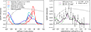Fig. 1. Left: Photometric redshift distributions of the photometric LBG samples UNIONSlike_RF in red (the convolution of the UNIONSlike_RF distribution with the DESI spectroscopic efficiency is shown in dashed and dotted lines, they have not been normalized to show the impact at z ∼ 2.5). The distribution of the samples UNIONSlike_RF_u180s, and LSSTY4like_RF_u2x180s are shown in blue and dashed cyan lines. Right: Photometric redshift distributions of the UNIONS LBG samples UNIONS_colorcut and UNIONS_PZcut in the XMM field. The sample selected with the hybrid method à-la SOM is shown for illustration. We also show the quantity nb (the product between the large-scale bias and the normalized redshift distribution) resulting from our clustering-redshift calibration methods.

Moreover, lensing magnification alters the observed galaxy number density by deflecting light from intervening structures. Depending on the survey flux limit and the slope of the luminosity function, this effect can lead to either an apparent enhancement or suppression of number counts. The associated kernel is given by

$$\begin{array}{c}\hfill q_{\mathrm{g}}^{\mathrm{mag}}(\chi )=(5s-2)\frac{3{\mathrm{\Omega }}_{\mathrm{m}}{H}_0^2}{2}\frac{\chi }{a(\chi )}{\int }_{\chi }^{{\chi }_{\mathrm{H}}}d\chi \prime n(z(\chi \prime ))\frac{\chi \prime -\chi }{\chi \prime }·\end{array}$$(3)

The above equation considers the leading-order magnification term¹, where s(m_lim, z) = dlog₁₀N(< m_lim, z)/dm (see Eq. (38) in Challinor & Lewis 2011) denotes the magnification bias² (Euclid Collaboration: Lepori et al. 2022; Elvin-Poole et al. 2023). We emphasize that it is a zeroth-order approximation of the magnification bias since color cuts may distort the effective selection at the limit magnitude m_lim. For the latter, we will consider the r band to compute the limiting magnitude of the sample. Although s(m_lim, z) shows some redshift dependence for the LBG samples used in this work (see Appendix C), we adopt a single value for the magnification bias, s(m_lim), defined as the average over redshift. This choice is motivated by the large uncertainties associated with the inferred redshift-dependent estimates for some samples. Moreover, redshift-space distortions (RSD) arise from the peculiar velocities of galaxies along the line of sight, which modify their observed redshifts and induce anisotropies in the observed clustering. The RSD kernel is given by

$$\begin{array}{c}\hfill q_{\mathrm{g}}^{\mathrm{RSD}}(\chi )=-H(z)n(z)\frac{\mathrm{d}lnD(a)}{\mathrm{d}lna}j{″}_{\ell }(k\chi ),\end{array}$$(4)

where D(a) is the linear growth factor and j_ℓ(x) is the ℓ-spherical Bessel function. From this, the observed angular power spectrum of the galaxy density field is given by

$$\begin{array}{c}\hfill C_{\ell }^{gg,\mathrm{obs}}=\sum _{\mathit{ij}}{C}_{\ell }^{q_i{q}_j}+\frac{1}{{\overline{n}}_{\mathrm{gal}}},\end{array}$$(5)

where $q_i\in \{q_{\mathrm{g}}^{\mathrm{int}},q_{\mathrm{g}}^{\mathrm{RSD}},q_{\mathrm{g}}^{\mathrm{mag}}\}$, and ${\overline{n}}_{\mathrm{gal}}$ is the surface density of the galaxy sample in steradians.

2.2. CMB Lensing and Cross-Correlation with LSS

The temperature anisotropies and polarization patterns of the CMB are gravitationally lensed by the intervening large-scale structure between the surface of last scattering and the observer. This lensing potential remaps the primary CMB anisotropies and induces B-mode polarization, as well as characteristic non-Gaussian features in the observed CMB maps (Lewis & Challinor 2006). The associated convergence field $\kappa (\widehat{\mathbf{n}})=-\frac{1}{2}{\mathrm{\nabla }}^2\varphi (\widehat{\mathbf{n}})$ can then be reconstructed from high-resolution CMB temperature and polarization maps using quadratic estimators (Okamoto & Hu 2003). The lensing convergence has a projection kernel given by

$$\begin{array}{c}\hfill q_{\kappa }(\chi )=\frac{3H_0^2{\mathrm{\Omega }}_{\mathrm{m}}}{2c^2}\frac{\chi }{a(\chi )}\left(\frac{{\chi }_{\ast }-\chi }{{\chi }_{\ast }}\right),\end{array}$$(6)

where χ_* is the comoving distance to the surface of last scattering, a(χ) is the scale factor, H₀ is the Hubble constant, and Ω_m is the matter density parameter today. This kernel peaks at redshift z ∼ 2, which makes CMB lensing especially sensitive to the high-redshift Universe.

The reconstructed CMB lensing convergence power spectrum includes both signal and noise contributions, and is given by C_ℓ^κκ, obs = C_ℓ^κκ + N_ℓ^κ where C_ℓ^κκ is the theoretical lensing auto-spectrum, and N_ℓ^κ is the lensing reconstruction noise, which depends on the specifications of the CMB experiment (e.g., angular resolution, instrumental noise, etc.). In this work, we adopt the noise spectrum of the CMB lensing maps derived from the Planck PR4 temperature and polarization data (Carron et al. 2022).

The CMB lensing signal can also be cross-correlated with the distribution of galaxies or other tracers of large-scale structure. Such cross-correlations provide a powerful probe of the large-scale matter distribution and the galaxy bias, and are sensitive to primordial non-Gaussianity, $f_{\mathrm{NL}}^{\mathrm{loc}}$, via scale-dependent effects. The observed cross-angular power spectrum between the CMB lensing field and a galaxy field is given by the sum of C_ℓ^κq_i, where the sum runs over the relevant galaxy kernel contributions q_i (i.e., intrinsic clustering, magnification, and redshift-space distortions).

2.3. PNG: impact of $f_{\mathrm{NL}}^{\mathrm{loc}}$ on galaxy field

Multifield inflation models can generate a small level of local PNG, parametrized by $f_{\mathrm{NL}}^{\mathrm{loc}}$, which modifies the statistics of the initial gravitational potential. By modifying the height of rare density peaks, the parameter $f_{\mathrm{NL}}^{\mathrm{loc}}$ alters the response of halo abundance to long-wavelength background modes, thereby affecting the large-scale halo bias (Dalal et al. 2008; Slosar et al. 2008; Desjacques & Seljak 2010). The tracer bias acquires an additional scale-dependent correction b → b + Δb in Eq. (2), with

$$\begin{array}{c}\hfill \mathrm{\Delta }b(z,k)=b_{\mathrm{\Phi }}{f}_{\mathrm{NL}}^{\mathrm{loc}}\frac{3{\mathrm{\Omega }}_{\mathrm{m}}{H}_0^2}{2k^{2}T(k)D(z)},\end{array}$$(7)

where T(k) is the matter power spectrum transfer function and D(z) is the linear growth factor. The bias b_Φ can be related to the linear tracer bias through the relation

$$\begin{array}{c}\hfill b_{\mathrm{\Phi }}=2(b(z)-p_{\mathrm{\Phi }}){\delta }_c,\end{array}$$(8)

where p_Φ = 1 is adopted for the universal mass function. While this relation is by far the most widely adopted in the literature, there is no compelling reason to expect it to hold for realistic tracers of large-scale structure. For instance, p_Φ = 1.6 yields a better description of b_Φ for objects whose host halos had recently undergone a major merger, such as quasar’s host halos (Slosar et al. 2008). In addition, p_Φ ∈ [0.4, 0.7] was found to describe accurately stellar mass-selected galaxies (Barreira et al. 2020). It is therefore generally accepted that p_Φ ≠ 1 must be taken into account depending on the tracer under consideration. Even if the lensing-related quantities are in principle subject to corrections from primordial non-Gaussianity (Jeong et al. 2011; Anbajagane et al. 2024), we neglect the impact of $f_{\mathrm{NL}}^{\mathrm{loc}}$ on the CMB lensing potential since the effects of $f_{\mathrm{NL}}^{\mathrm{loc}}$ are strongly suppressed by projection effects. Thus, in this work, we rely on the large-scale dependent bias effect described in Eq. (7) to constrain $f_{\mathrm{NL}}^{\mathrm{loc}}$.

3. Datasets

In this work, we perform a forecast study for an LBG sample that can be generated from the UNIONS data. The UNIONS is build upon a collaboration between the Hawaiian observatories: the Canada-France-Hawaii Telescope (CFHT, Mauna Kea), the Panoramic Survey Telescope and Rapid Response System (Pan-STARRS, Maui), and the Subaru Telescope (Mauna Kea). It is currently providing ugriz imaging over 5000 deg² of the northern sky. The CFHT Canada-France Imaging Survey (CFHT/CFIS) targets the u and r bands with the Megacam imager, delivering image quality competitive with all other current large ground-based facilities. CFHT/CFIS will reach a depth of r ≃ 25 over 5000 deg² and u ≃ 24.6 over 9000 deg². Meanwhile, Pan-STARRS provides the i-band, and the Wide Imaging with Subaru Hyper Suprime-Cam of the Euclid Sky (WISHES) supplies the z-band. The 5σ depth of the data, measured within a 2-arcsecond diameter aperture (Gwyn et al. 2025), is [u, g, r, i, z]=[24.45, 25.25, 24.95, 24.55, 24.05]. Multiband catalogs over the UNIONS footprint have been obtained using the GAaP (Gaussian Aperture and PSF; Kuijken 2008; Kuijken et al. 2015, 2019) method, which will be made publicly available upon release of the UNIONS data set. The covered surface areas are, for {ugr, ugri, ugriz}={4760, 4630, 3730} deg² (Gwyn et al. 2025). Besides the main UNIONS footprint, multiband ugr catalogs are available on the two deep fields XMM-LSS and COSMOS. We will consider using these deep fields in the next section.

In the following sections, we present the various LBG selections applied to UNIONS-like and UNIONS imaging. For each case, we derive the corresponding sample characteristics, namely the redshift distribution and the lensing magnification bias.

3.1. UNIONS-like LBG sample from a Random Forest approach by degrading deep catalogs

In this section, we present the selection of high-redshift LBGs on UNIONS-like imaging, obtained on the COSMOS field.

3.1.1. Photometric LBG sample:

We first introduce the LBG sample that was derived in Payerne et al. (2025), labeled as UNIONSlike_RF, obtained by applying a Random Forest selection to UNIONS-like photometry, i.e., by degrading CLAUDS³u and HSC⁴-PDR3 griz broadband imaging on the COSMOS field. For this dataset, we get deep 5σ point source depth [u, g, r, i, z]=[27.7, 27.4, 27.1, 26.9, 26.3]. The combination of CLAUDS and HSC-SSP data over COSMOS (and other small deep fields such as XMM-LSS) is detailed in Desprez et al. (2023). In Payerne et al. (2025), the COSMOS CLAUDS+HSC catalog has been degraded to UNIONS depth (called UNIONS-like, with respective depth, at the time of this work ugriz = [24.6, 25.5, 25.5, 24.2, 24.4], see Appendix E.2 for more details on this method) to train a Random Forest for selecting r < 24.3 UNIONS-like LBGs in the redshift range z ∈ [2.5, 3.5]. The LePhare (6 bands) photometric redshift distribution of this sample is shown in red full lines in the left panel of Figure 1, corresponding to a surface density of ∼1100 photometric LBGs per deg². The magnification bias factor for this sample is found to be s(r_lim = 24.3) = 0.43. As mentioned in Payerne et al. (2025), the artificial degradation procedure to mimic shallower depths is valid for point-source magnitude rescaling (which may be different for some galaxy populations), simplified noise models (decreasing the photon count only) thus neglects several sources of systematic uncertainty inherent to each photometric pipelines; it should therefore be regarded as an optimistic approximation of shallower imaging conditions. In addition, the Random Forest model is trained on relatively small datasets (the COSMOS and XMM-LSS fields are of a few square degrees), which may limit its ability to capture rare populations and increase sensitivity to statistical fluctuations due to large-scale survey systematics (depth coverage, etc.) and sample variance.

3.1.2. DESI-II LBG sample:

This work is also the occasion to explore DESI-II scenarios, whose high-redshift target selection strategy is still under discussion. Spectroscopic redshift follow-ups will allow us to (1) remove low redshift contaminants and (2) reduce the uncertainty on the sample redshift distribution. Considering all z > 2 objects in the distribution in Figure 1 (left panel), the number density goes from 1100 to 880 LBGs per square degree. Moreover, the current DESI spectroscopic redshift reconstruction method⁵ has an internal efficiency, which degrades the efficiency of the recovered LBG spectroscopic sample at z ∼ 2.2. Considering the redshift efficiency in Figure 11 of Payerne et al. (2025) or in Fig. 18 of Ruhlmann-Kleider et al. (2024) (resp. for 2-hour and 4-hour exposure) multiplying the corresponding redshift distribution, we get the corrected number densities 500 and 590 LBGs per square degrees. The corresponding 2-hour and 4-hour exposure high-redshift distributions are shown in the left panel of Figure 1.

3.1.3. Alternative LBG selection:

We explore two alternative UNIONS-like LBG selections on the COSMOS field; Individual CLAUDSu-band images of 180-second exposures on COSMOS have been coadded and have undergone forced photometry using HSC g-band. Two u-band catalogs were obtained, corresponding to 180-second and 2 × 180-second exposures (see Appendix E.1). For reference, the default deep CLAUDSu-band catalog uses 600-second exposures. Two other selections, namely UNIONSlike_RF_u180s and LSSTY4like_RF_u2x180s where obtained by training a RF algorithm to select a sample of 1100 deg⁻² galaxies with r < 24.5 in the range z ∈ [2.5, 3.5], where, for each galaxy sample, s(r_lim = 24.5) = 0.21 and 0.46, respectively. The corresponding photometric redshift distributions are represented in the left panel of Fig. 1. These selections, as for the one in Payerne et al. (2025), were tested on the COSMOS field and show different selection efficiencies.

3.2. LBG sample using UNIONS GAaP catalogs

In this section, we make use of the early GAaP UNIONS data to test different high-redshift LBG selections.

3.2.1. LBG color-color selection

We use the early UNIONS GAaP photometric data available in the UNIONS collaboration, to test a color–color box selection of high-redshift r < 24.2 LBGs referred to as [COSMOS: TMG u dropout] in Ruhlmann-Kleider et al. (2024) (see their Table 1). For 22 < r < 24.2, the u-dropout color selection is defined as

$$\begin{array}{cc}& (\mathrm{i})u-g>0.3,\hfill \end{array}$$(9)

$$\begin{array}{cc}& (\mathrm{ii})-0.5<g-r<1,\hfill \end{array}$$(10)

$$\begin{array}{cc}& (\mathrm{iii})[u-g>2.2\times (g-r)+0.32]\hfill \end{array}$$(11)

$$\begin{array}{cc}& \cup [u-g>0.9\cap u-g>1.6\times (g-r)+0.75].\hfill \end{array}$$(12)

This sample is referred to as UNIONS_colorcut and yields a photometric LBG angular density of 1400 deg⁻² and a magnification bias s(r_lim = 24.2) = 0.25. To assess the redshift distribution of these photometrically selected u-dropout LBGs, we match geometrically the selected UNIONS-LBGs to deep photometric redshift catalogs provided by CLAUDS+HSC imaging on XMM (XMM benefits from UNIONS multiband imaging). The corresponding photometric redshift distribution is displayed in the right panel of Figure 1. In our previous Payerne et al. (2025) idealistic dataset, the resulting redshift distribution n(z) is relatively narrow, peaking sharply at z ∼ 3. In comparison to the color-box selection, which peaks at z ∼ 1.5 with a broader shape, the difference reflects (i) the slight optimistic ugrz magnitude depth used in Payerne et al. (2025) for the degradation procedure (ii) the use of a Random Forest approach (iii) the simplified and noise-free nature of the simulated conditions in Payerne et al. (2025), where measurement uncertainties, selection effects, and intrinsic galaxy diversity are minimized. The broadening of the UNIONS distribution can be attributed to observational noise in UNIONS data, all of which introduces scatter and extends the distribution away from the main peak. As a result, the realistic dataset provides a more accurate representation of the complexity encountered in real observations.

As for the idealistic Payerne et al. (2025), an alternative is to use a Random Forest classifier to select LBGs within a specific redshift range using UNIONS imaging. However, the limited overlap between UNIONS and CLAUDS+HSC on XMM restricts the available training data (the overlap is about 2 deg²). Instead, we construct a hybrid selection by splitting the matches into two separate samples. For the first subsample, we precompute the mean LePhare photometric redshift in a multidimensional grid of UNIONS colors (u − g, g − r, r − i) and r magnitude. A UNIONS galaxy in the second subsample is considered as part of the LBG sample if the mean redshift in its associated grid cell satisfies ⟨z⟩> 1.7. This grid-based approach is conceptually similar to Self-Organizing Maps (SOMs, Zhang et al. 2025; Roster et al. 2026), and poorly mimics the cut-free approach of Random Forests. From this, we obtain a representative redshift distribution based on a reference sample. Our method uses a fixed, axis-aligned grid, while SOMs construct an adaptive, data-driven grid that captures complex structures in color space. This hybrid SOM-like selection tests the relevance of the color-box cuts compared to a data-driven cut-free method, which is represented in green in the right panel of Figure 1. We observe that the distribution fairly matches the color-color box selection.

To check the consistency of the u-dropout selection described above, we apply an alternative selection based on the BPZ photometric redshifts (Benítez 2011) of UNIONS detections, requiring Z_ML > 1.7 in the catalog. This selection is referred to as UNIONS_PZcut, and represented in purple in the right panel of Figure 1. This validation on XMM of the color-box selection enables us to apply this selection to a wider UNIONS portion of the sky, and assess the corresponding redshift distribution through clustering-redshift methods.

3.2.2. Measuring the redshift distribution of u-dropout LBGs

Matching LBG targets with deep CLAUDS+HSC photometric catalogs is useful to assess the underlying photometric redshift distribution; however, this approach remains limited by the accuracy of the deep photometric catalogs and by the relatively low statistical significance of the inferred distribution (usually done on fields of a few square degrees). A second method relies on spectroscopic data, as high-precision spectroscopic measurements can help calibrate the less accurate photometric redshifts. For available spectroscopic subsamples of photometric datasets, direct calibration is possible (see, e.g., Lima et al. 2008; Hildebrandt et al. 2021). Such direct calibration is challenging for LBGs, however, since obtaining a representative spectroscopic sample for any specific photometric selection is difficult in practice (Ruhlmann-Kleider et al. 2024; Payerne et al. 2025).

In this work, we use the clustering-redshifts method (Ménard et al. 2013; Schmidt et al. 2013; d’Assignies et al. 2025b) to evaluate the redshift distribution of an arbitrary photometrically-selected dataset based on the spatial cross-correlation with a reference population, the latter with spectroscopic redshift available. The overlap of UNIONS data we use in this work with DESI spectroscopic observations publicly available (DR1, Ross et al. 2025) is approximately 1300 deg². The region of overlap suffers from a low completeness of DESI data (Dec > 30 deg), which limits the method’s constraining power. DESI data also includes randoms. We evaluate the measurements for the different DESI tracers separately (BGS, LRG, ELG, and QSO), and then recombine them, as the tracers’ masks differ from one to another. The DESI data are then used to measure the product of the redshift distribution with galaxy bias b_LBG(z) n_LBG(z) with the so-called clustering-redshifts methods (using the pipeline developed in d’Assignies et al. 2025b), over the redshift range 0 < z < 3.4. Contrary to the majority of the previous clustering-redshift calibration methods, we do not aim to break the degeneracy between bias and redshift distribution, as the observables we consider directly depend on their product. The uncertainty σ(b_LBG(z) n_LBG(z)) can then be used directly for the Bayesian inference, and we marginalize over both bias and distribution during the same step.

For clustering-redshift calibration, we binned the spectroscopic data in redshift bins z_j ± Δz/2, and measure the cross correlations between each spectroscopic bin s_j and the UNIONS LBG bin, as functions of perpendicular separations r_p: w_sj LBG(r_p). To maximize the signal-to-noise ratio and simplify covariance estimates, we usually reduce the data vectors to scalars given by

$$\begin{array}{c}\hfill {\overline{w}}_{{\mathrm{s}}_j\mathrm{LBG}}={\int }_{r_{\mathrm{p},\min }}^{r_{\mathrm{p},\max }}W(r_{\mathrm{p}})w_{{\mathrm{s}}_j\mathrm{LBG}}(r_{\mathrm{p}})\mathrm{d}{r}_{\mathrm{p}},\end{array}$$(13)

with W(r_p)∝r_p^γ a normalized weighting functions. We use the scale range 1.5 − 5.5 Mpc and the weighting γ = −1, which is an excellent tradeoff between boosting the signal-to-noise ratio coming from small scales, limiting biasing due to nonlinearity (d’Assignies et al. 2025b), and fiber collisions (see Choppin de Janvry et al. 2025; d’Assignies et al. 2025a). These scalars can be used to constrain b_LBG(z) n_LBG(z) as

$$\begin{array}{c}\hfill b_{\mathrm{LBG}}(z_j)n_{\mathrm{LBG}}(z_j)=\frac{{\overline{w}}_{{\mathrm{s}}_j\mathrm{LBG}}}{b_{\mathrm{r}}(z_j){\overline{w}}_{\mathrm{m}}(z_j)},\end{array}$$(14)

where ${\overline{w}}_{\mathrm{m}}$ is a theoretical function estimated with Halofit (Takahashi et al. 2012). The spectroscopic galaxy biases b_s(z_j) are measured from the auto-correlations of the spectroscopic bins, for larger scales (to limit the effect of fiber collision). The data vectors are measured with Treecorr (Jarvis 2015) and LS estimators (Landy & Szalay 1993). Moreover, the correlations of $\overline{w}$ between different redshifts z_j can be neglected (d’Assignies et al. 2025a). Thus, we estimate the covariance matrix using a standard Jackknife estimate, and set all the off-diagonal coefficients to 0. We combined the measurements from different tracers localized at the same redshift, using an inverse weighting scheme, neglecting cross-correlations (Choppin de Janvry et al. 2025). The joint product of the LBG bias and the LBG redshift distribution in Eq. (14) is shown in Figure 1 (right panel) with the corresponding error bars. For the latter, we work in a minimal scenario, where the bias and the redshift distribution cannot be disentangled. This is possible by dealing with accurate photometric redshifts. We can compute an effective bias of the sample by integrating b_LBGn_LBG, we get b_eff = 1.5 ± 0.2, where the error is estimated from random samples of b_LBG n_LBG.

We will use clustering-redshift estimates of b_LBGn_LBG for a subset of the forecasts, propagating the associated uncertainties, arising from imperfect knowledge of the galaxy bias and redshift distribution, to illustrate a data-driven forecast scenario. Owing to the limited sky overlap, these estimates carry relatively large uncertainties.

4. Modeling of LBG properties

We first detail how to parametrize uncertainties associated with our LBG sample, i.e., the large-scale bias, the outlier fraction, and the redshift distribution uncertainty, as well as accounting for clustering-redshift-derived distribution in the $f_{\mathrm{NL}}^{\mathrm{loc}}$ prediction.

4.1. Modeling of the LBG large-scale linear bias

For the galaxy large-scale bias, we follow (Wilson & White 2019)

$$\begin{array}{c}\hfill b_{\mathrm{W}19}(z,m)=A(m)(1+z)+B(m){(1+z)}^2,\end{array}$$(15)

with A(m) = − 0.98 (m − 25)+0.11 and B(m) = 0.12 (m − 25)+0.17. Here, m is the apparent magnitude, to be considered to be the limiting magnitude m_lim of the LBG sample (d’Assignies et al. 2023). For u-dropout (resp. g-dropout and r-dropout) LBGs, the limiting magnitude corresponds to the r band (resp. i and z band). This prescription successfully reproduces the large-scale bias measurements for various dropout selections and limiting magnitudes from the CARS⁶ (Hildebrandt et al. 2009) and GOLDRUSH⁷ (Ono et al. 2018) surveys. For the UNIONSlike_RF, UNIONSlike_RF_u180s, UNIONSlike_RF_u2x180s and UNIONS_colorcut samples, we use m_lim = 24.3, 24.5, 24.5 and 24.2, respectively⁸. We introduce a global rescaling amplitude b₀, so that the LBG bias is modeled as

$$\begin{array}{c}\hfill b(z)=b_0\times b_{\mathrm{W}19}(z,m_{\lim }).\end{array}$$(16)

4.2. Fraction of LBG outlier and their galaxy bias

In this section, we expect our LBG samples to be contaminated by a fraction f_out of outliers, from which we can define a proper large-scale linear bias. We use a two-population model for a given sample with given total n(z), with some outliers at redshift z < z_mid with given redshift distribution n_out(z), outlier fraction f_out and bias b_out(z), along with a high-redshift sample at z > z_mid, with redshift distribution n_highz(z) and bias b_highz(z), such as

$$\begin{array}{c}\hfill n(z)=f_{\mathrm{out}}{n}_{\mathrm{out}}(z)+(1-f_{\mathrm{out}})n_{\mathrm{high}z}(z).\end{array}$$(17)

The values taken for f_out are discussed later in Section 6.1.4. We adopt the two-population bias model (Mergulhão et al. 2022)

$$\begin{array}{c}\hfill b(z)=b_0\times [b_1(z)+b_2(z)],\end{array}$$(18)

where

$$\begin{array}{c}\hfill (b_1,b_2)=(\frac{f_{\mathrm{out}}{n}_{\mathrm{out}}(z)b_{\mathrm{out}}(z)}{n(z)},\frac{(1-f_{\mathrm{out}})n_{\mathrm{high}z}(z)b_{\mathrm{high}z}(z)}{n(z)}).\end{array}$$(19)

Moreover, we also use the model

$$\begin{array}{c}\hfill b(z)=b_1(z)+b_0\times b_2(z),\end{array}$$(20)

where this time, b₀ is connected only to the high-redshift portion of the sample, contrary to Eq. (18). As a result, only the high-redshift LBG bias is treated as unknown, and the uncertainty on $f_{\mathrm{NL}}^{\mathrm{loc}}$ is expected to be smaller than in the previous case, since the low-redshift outlier bias is fixed.

4.3. LBG redshift distribution uncertainty

Cosmological inference from the angular clustering of photometrically selected u-dropout LBGs relies on an accurate determination of their redshift distribution, n(z) (Choi et al. 2016; Petri et al. 2026). Calibrated n(z) has error bars that translate the uncertainty in calibrating the redshift distribution of LBGs. We consider a very simple toy example where the LBG sample has a n(z) with error bar σ(z). To propagate the uncertainty of the n(z) on the cosmological fits, we consider random samples ${\widehat{n}}_k\sim \mathcal{N}(n(z),\sigma (z))$, where σ(z) is taken to be αn(z), i.e., a fraction of the total n(z). We consider α = 0.2 (i.e., 20% error on the recovered redshift distribution). We explore another n(z)-sampling technique, inspired from the shift-and-stretch standard method in the literature (Myles et al. 2021; d’Assignies et al. 2025b; Giannini et al. 2025), where we shift the high-redshift part of the Payerne et al. (2025)n(z) (left panel of Figure 1), i.e., z > 1 part around its mean z = 2.8 by a factor Δz ∼ 𝒩(0, 0.1), and stretch it by a factor 1 + α ∼ 𝒩(1, 0.1).

4.4. Accounting for all with Cz estimates

The clustering-redshift method estimates the product ⟨b_LBGn_LBG⟩(z), directly accounting for outliers. This inherent degeneracy between b(z) and n(z) cannot be disentangled without highly precise UNIONS photometric redshifts, making it practically impossible to separate the two terms n(z) and b(z). For standard galaxy clustering analysis, this is indeed advantageous, as marginalizing over clustering redshift uncertainties accounts for both the redshift evolution of the distribution and bias, as the degeneracy between b and n is also in the intrinsic kernel, cf. Eq. (2). As we are considering an additional term from non-Gaussianity, we slightly modify the kernel in Eq. (7) with

$$\begin{array}{c}\hfill b_{\mathrm{LBG}}{n}_{\mathrm{LBG}}(z)[1+2{\delta }_c(1-\frac{p}{b_{\mathrm{eff}}})f_{\mathrm{NL}}^{\mathrm{loc}}\frac{3{\mathrm{\Omega }}_{\mathrm{m}}{H}_0^2}{2k^{2}T(k)D(z)}],\end{array}$$(21)

where b_eff = 1.5, as computed previously. That way, $f_{\mathrm{NL}}^{\mathrm{loc}}$ is to be the only free parameter of the fit, as redshift uncertainty on bias and distribution, and outlier fraction are accounted for in the nb term. However, we are neglecting the impact of the redshift evolution on the galaxy bias in the second term. Let’s note that the form of the second term is, on its own, not exact, as we are also assuming a specific (and redshift invariant) model for b_ϕ.

We further explore a more sophisticated bias modeling, adopting the prescription of Wilson & White (2019) used throughout this work. In this case, b₀ is no longer a free parameter but is instead fixed by the normalization constraint

$$\begin{array}{c}\hfill {\overline{b}}_0={\int }_0^{+\infty }\mathrm{d}z\prime \frac{b_{\mathrm{LBG}}{n}_{\mathrm{LBG}}(z\prime )}{b_{\mathrm{W}19}(z\prime )}=0.63.\end{array}$$(22)

From this, we replace b_eff in Eq. (21) by ${\overline{b}}_0{b}_{W19}(z)$, incorporating redshift dependence in LBG bias.

5. Forecasting methodology

In our forecast analysis, we consider two free parameters: (i) $f_{\mathrm{NL}}^{\mathrm{loc}}$, with a fiducial value of 0, and (ii) a galaxy bias-related parameter b₀ (see below), rescaled to 1 as its fiducial value. To forecast constraints on $f_{\mathrm{NL}}^{\mathrm{loc}}$, we consider the observed dataset as a theoretical prediction for the clustering amplitudes of the LBG population and the CMB lensing potential, along with the corresponding theoretical covariances. In other words, the data we use in the forecasts are the binned theoretical predictions ${\{C_b^{gg,\mathrm{obs}},C_b^{\kappa g,\mathrm{obs}}\}}_{(b_0,f_{\mathrm{NL}}^{\mathrm{loc}})=(1,0)}$ where C_b^XY = B_bℓ C_ℓ^XY, B_bℓ is the binning matrix. We adopt a binning scheme inspired by Krolewski et al. (2024), with ℓ_min = 5 (this lower limit is also imposed by the UNIONS sky coverage), ℓ_max = 300 (safely describing galaxy clustering statistics as linear and redshift-only bias dependent), and Δℓ = 5, resulting in 60 bins. In the above equation, C_ℓ^XY is the unbinned full-sky angular power spectrum in multipole ℓ bins. Using the theoretical full-sky prediction is appropriate because it eliminates the variance of the estimator, resulting in a posterior distribution centered on the input values. However, this approach is a simplification, as it does not account for potential systematic biases in the signal estimation pipeline, which must be corrected in the analysis (e.g., via radial integral constraints).

The covariance of the binned de-coupled angular power spectrum is given by

$$\begin{array}{c}\hfill \mathrm{Cov}({\widehat{C}}_b^{\mathit{XY}},{\widehat{C}}_{b^{\prime }}^{\mathit{ZW}})=B_{b\ell }\mathrm{Cov}({\widehat{C}}_{\ell }^{\mathit{XY}},{\widehat{C}}_{{\ell }^{\prime }}^{\mathit{ZW}})B_{b^{\prime }{\ell }^{\prime }},\end{array}$$(23)

where B_bℓ is the binning matrix, and the covariance of the unbinned spectra is (Brown et al. 2005)

$$\begin{array}{c}\hfill \mathrm{Cov}({\widehat{C}}_{\ell }^{\mathit{XY}},{\widehat{C}}_{{\ell }^{\prime }}^{\mathit{ZW}})=\frac{C_{\ell }^{\mathit{XZ}}{C}_{\ell }^{\mathit{YW}}+C_{\ell }^{\mathit{XW}}{C}_{\ell }^{\mathit{YZ}}}{2\ell +1}{\mathcal{M}}_{\ell {\ell }^{\prime }}^{-1},\end{array}$$(24)

where ℳ_ℓℓ′⁻¹ is the mixing-mode matrix which accounts for partial sky coverage (Alonso et al. 2019). Not included in our mock validation pipeline are non-Gaussian contributions to the covariance, such as the super-sample covariance (SSC), which is currently considered to be the dominant non-Gaussian contribution. SSC arises from the non-linear modulation of local observables by long-wavelength density fluctuations.

For our inference, we then adopt the theoretical data vector (i.e., the input prediction for the angular power spectrum), which is satisfactorily recovered by the mocks, along with the theoretical covariance that includes the full mode-coupling matrix. We also include a free galaxy bias-related parameter, b₀, with a default value of 1, used to rescale certain LBG bias dependencies (discussed below). For the measured LBG angular power spectrum, the cross-angular power spectrum between the LBG density and the CMB lensing, and for the combination of the two, the likelihoods (respectively, ℒ_gg, ℒ_κg, ℒ_gg + κg) are assumed to follow a multivariate Gaussian distribution with theoretical covariances computed at the fiducial values $(f_{\mathrm{NL}}^{\mathrm{loc}},b_0)=(0,1)$, which is accurate for approximating the likelihood of angular power spectra, which follows a Gamma distribution (Carron 2013).

We then draw samples from the parameter posterior distribution using Bayes’ theorem:

$$\begin{array}{c}\hfill \mathcal{P}(\theta |\mathrm{data})=\frac{{\mathcal{L}}_{\mathrm{tot}}(\mathrm{data}|\theta )\pi (\theta )}{{\mathcal{L}}_{\mathrm{tot}}(\mathrm{data})},\end{array}$$(25)

where ℒ_tot corresponds to ℒ_gg, ℒ_κg, or ℒ_gg + κg. We use the emcee package (Foreman-Mackey et al. 2013) with flat priors on $f_{\mathrm{NL}}^{\mathrm{loc}}$ (between −500 and 500) and b₀ (between 0 and 5). To accelerate the likelihood evaluation, we adopt the template method presented in Fabbian et al. (2026); Since our goal is to infer the LBG linear bias and the PNG parameter $f_{\mathrm{NL}}^{\mathrm{loc}}$, most contributions to the angular power spectra arise from pre-factors $(b_0,f_{\mathrm{NL}}^{\mathrm{loc}})$ multiplying terms that are independent of bias and PNG. This is always the case for $f_{\mathrm{NL}}^{\mathrm{loc}}$, and for b₀ when it simply rescales the overall bias of the considered population. We precompute the angular power spectra for a fiducial cosmology with $f_{\mathrm{NL}}^{\mathrm{loc}}=0$ and with b₀ = 1, allowing only b₀ and $f_{\mathrm{NL}}^{\mathrm{loc}}$ to vary in the MCMC. This approach reduces the computation time of each likelihood evaluation to a few milliseconds and posterior estimations in seconds. The recovered uncertainties on $f_{\mathrm{NL}}^{\mathrm{loc}}$ and b₀ are taken to be the standard deviations of the recovered posterior distributions.

When accounting for redshift distributions in the inference, a continuous model that can be readily marginalized over is often unavailable. On the other hand, generating realizations of n(z) is usually straightforward (see Sections 4.3 and 4.4). This is typically the situation described in Bernstein et al. (2025), except that we are dealing with only one bin at a time and our likelihood can be evaluated within milliseconds. Hence, we can directly compute the likelihood for every discrete realization n_k and effectively marginalize over them by stacking:

$$\begin{array}{c}\hfill \mathcal{L}(x|y)\approx \frac{1}{N_{\mathrm{real}}}\sum _k\mathcal{L}(x|y,n_k),\end{array}$$(26)

where N_real is the number of realizations, all assumed to have equal probability, independent of y.

6. Results on $f_{\mathrm{NL}}^{\mathrm{loc}}$ precision

6.1. From UNIONS-like LBG samples

The constraining power on $f_{\mathrm{NL}}^{\mathrm{loc}}$ from galaxy two-point statistics arises primarily from the largest clustering scales (i.e., the lowest multipoles ℓ). The gain in $f_{\mathrm{NL}}^{\mathrm{loc}}$ precision enabled by the increased LBG density from UNIONS is only realized if the relevant scales of C_ℓ^gg are in the shot-noise-dominated regime. In the cosmic-variance–dominated regime, where $C_{\ell }^{\mathit{gg}}\gg 1/\overline{n}$ or equivalently $C_{\ell }^{\mathit{gg}}\overline{n}\gg 1$, the improvement from a higher number density saturates. For C_ℓ^κg, the cosmic-variance–dominated regime requires both $C_{\ell }^{\mathit{gg}}\gg 1/\overline{n}$ and C_ℓ^κκ ≫ N_ℓ^κκ. In the lower plot of Figure 2, we show the quantities $C_{\ell }^{\mathit{gg}}\overline{n}$ and C_ℓ^κκ/N_ℓ^κκ. To define the cosmic-variance–dominated regime, we adopt the criteria $C_{\ell }^{\mathit{gg}}\overline{n}>10$ and C_ℓ^κκ/N_ℓ^κκ > 10. We find that the LBG auto-spectrum is cosmic-variance dominated up to ℓ ≲ 200, implying that increasing the tracer density does not improve the signal-to-noise ratio on these scales. At smaller scales, however, a higher tracer density can still provide additional information on the tracer bias, rather than directly on the $f_{\mathrm{NL}}^{\mathrm{loc}}$ response, thereby helping to break the degeneracy between b₀ and $f_{\mathrm{NL}}^{\mathrm{loc}}$.

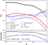Fig. 2. Top panel shows the angular power spectra Cℓgg, Cℓκg, and Cℓκκ (solid lines) for the baseline sample. The cosmological-only contribution is shown as dashed lines, while the noise contribution is shown as dotted lines. Bottom panel shows the signal-to-noise ratio, defined as the ratio of the cosmological-only term to the noise, for Cℓgg and Cℓκκ.

We first consider an idealized framework, with no outliers, no uncertainty, and with the redshift distribution set in Payerne et al. (2025) to evaluate the precision on $f_{\mathrm{NL}}^{\mathrm{loc}}$ and b₀ from a combination of the auto- and cross-spectra, C_ℓ^gg and C_ℓ^gκ, respectively. We obtain $\sigma (f_{\mathrm{NL}}^{\mathrm{loc}})=7$ from C_ℓ^gg alone. From C_ℓ^κg alone, the constraints are $\sigma (f_{\mathrm{NL}}^{\mathrm{loc}})=34$. The joint constraints (i.e., combining C_ℓ^gg and C_ℓ^κg) are very similar to those from C_ℓ^gg alone, reflecting the relatively larger uncertainties from the C_ℓ^κg-only case. The corresponding posterior distributions for the C_ℓ^κg-only and C_ℓ^gg-only analyses are shown in the left panel of Figure 3. Although we do not adopt a tomographic approach by splitting the LBG sample into different redshift bins (see, e.g., Fabbian et al. 2026; Chiarenza et al. 2025), we mention that this method – when tomographic redshift distribution are sufficient constrained – can help separate potential systematic effects affecting only a fraction of the sample by providing improved constraints on the galaxy bias in each redshift bin. In Appendix D, we find that splitting the LBG redshift distribution into three bins between z = 1.5 and z = 3.5 with roughly equal numbers of objects (around 300 deg⁻²) still results in a cosmic-variance dominated regime on the scales considered (with respect to the galaxy surface density), while significantly degrading the signal-to-noise of the cross-spectrum in each bin compared to a single-bin approach.

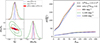Fig. 3. Left: Posterior distribution of the parameters $f_{\mathrm{NL}}^{\mathrm{loc}}$ and the large-scale linear bias (expressed in terms of relative error). Right: Forecasted error on $f_{\mathrm{NL}}^{\mathrm{loc}}$ as a function of the lower multipole cut ℓmin. Solid lines show constraints using only $C_{\ell }^{\kappa g}(\ell >{\ell }_{\min })$, while dashed lines correspond to the combination of $C_{\ell }^{\kappa g}$ and $C_{\ell }^{\mathit{gg}}(\ell >{\ell }_{\min })$. Different colors indicate different LBG number densities: 800, 1100, and 2000 LBGs per deg2.

While CMB lensing reconstruction from temperature data can be contaminated by extragalactic foregrounds such as the Cosmic Infrared Background and the thermal Sunyaev-Zel’dovich effect, a polarization-only CMB lensing map–despite its higher noise–can also be used to measure $f_{\mathrm{NL}}^{\mathrm{loc}}$ (Chiarenza et al. 2025). On the considered fitting scales, the Planck PR4 Polarization-only CMB lensing noise spectrum is 7 to 12 times larger than the Temperature+Polarization one. With Polarization-only noise, we get $\sigma (f_{\mathrm{NL}}^{\mathrm{loc}})=94$ (roughly $\sqrt{10}$ times larger than with Temperature+Polarization), with a 20% precision on the bias.

Table A.1 lists the forecasted precision on $f_{\mathrm{NL}}^{\mathrm{loc}}$ and b₀ for the various analysis cases we explore in this work. We also indicate to what percentage the $f_{\mathrm{NL}}^{\mathrm{loc}}$ constraints compare to the baseline constraints with the UNIONS-like RF LBG sample, which yields $\sigma (f_{\mathrm{NL}}^{\mathrm{loc}})=34$. We will now move to forecasts considering different modeling choices, treatment of uncertainties and systematics, cf. Section 4.

6.1.1. Impact of the angular momentum fitting range to mitigate imaging systematics

Imaging systematics, such as survey depth inhomogeneities and Galactic dust, can induce spurious density fluctuations in the tracer sample, generating artificial clustering signals. These effects are particularly problematic on the large scales most relevant for $f_{\mathrm{NL}}^{\mathrm{loc}}$ measurements, where they can lead to significant biases. A common mitigation strategy is to model the tracer density variations as linear functions of imaging properties and then reweigh the tracers, thereby suppressing spurious fluctuations while preserving the cosmological signal (Chaussidon et al. 2022; Krolewski et al. 2024). In the context of $f_{\mathrm{NL}}^{\mathrm{loc}}$ inference from the tracer angular power spectrum, however, removing such systematic contributions from the auto-spectrum C_ℓ^gg remains challenging. For this reason, angular power spectrum–based analyses often rely primarily on the cross-spectrum with CMB lensing, C_ℓ^κg, since the large-scale modes of C_ℓ^gg are the most contaminated. It is therefore important to explore the constraining power of the LBG angular distribution when used exclusively in cross-correlation with the CMB lensing potential.

In the right panel of Figure 3, we show the precision on $f_{\mathrm{NL}}^{\mathrm{loc}}$ obtained from C_ℓ^κg only, with fitting ranges ℓ ∈ [ℓ_min, 300] and 5 < ℓ_min < 200. As expected, the constraints rapidly degrade with increasing ℓ_min, since the sensitivity to $f_{\mathrm{NL}}^{\mathrm{loc}}$ resides on the largest clustering scales. In parallel, we show the constraints from a joint analysis of C_ℓ^κg and C_ℓ^gg, where the auto-spectrum is progressively truncated to ℓ ∈ [ℓ_min, 300], under the assumption that the clustering signal of C_ℓ^gg can be reliably recovered only for ℓ > ℓ_min. We find that as ℓ_min increases, the precision on $f_{\mathrm{NL}}^{\mathrm{loc}}$ approaches the C_ℓ^κg-only result. The corresponding posterior distribution for ℓ_min = 200 is shown in the left panel of Figure 3. While essentially no constraining power remains on $f_{\mathrm{NL}}^{\mathrm{loc}}$ in this case, the precision on the bias parameter b₀ is significantly improved. This indicates that relying on the small-scale clustering of the LBG population primarily constrains b₀, rather than $f_{\mathrm{NL}}^{\mathrm{loc}}$, since these scales are insensitive to primordial non-Gaussianity but probe the large-scale linear bias more efficiently. So far, we have discussed the constraining power on $f_{\mathrm{NL}}^{\mathrm{loc}}$ from the joint analysis of the LBG auto-power spectrum and the cross-correlation between LBGs and the CMB lensing map. In the next section, we instead focus on assessing the precision on $f_{\mathrm{NL}}^{\mathrm{loc}}$ using the cross-correlation alone, adopting a more conservative approach regarding the treatment of imaging systematics.

6.1.2. Impact of the b_Φ(b) parametrization

The sensitivity of the angular power spectrum to $f_{\mathrm{NL}}^{\mathrm{loc}}$ is entirely degenerate with the parameter b_Φ, through the combination $b_{\mathrm{\Phi }}{f}_{\mathrm{NL}}^{\mathrm{loc}}$ in Eq. (7). In the previous section, we assumed the universality of the halo mass function, which allows a partial disentanglement of $f_{\mathrm{NL}}^{\mathrm{loc}}$ from the LBG bias via the b_Φ(b) relation in Eq. (8). For most real tracers of large-scale structure, however, this universality does not hold, and the relation must account for a parameter p_Φ that encodes the tracer’s merger history (Slosar et al. 2008), with p_Φ = 1 corresponding to the universal case. The parameter p_Φ remains poorly constrained across tracer populations, and broad marginalization over it can degrade $f_{\mathrm{NL}}^{\mathrm{loc}}$ estimates (Barreira 2020). In the absence of reliable priors on p_Φ, only the combination $b_{\mathrm{\Phi }}{f}_{\mathrm{NL}}^{\mathrm{loc}}$ can be constrained, although any nonzero detection of this product would still indicate the presence of local primordial non-Gaussianity. Besides the fiducial value p_Φ = 1, we consider several alternative values from 0.1 to 2. Using the bias prescription in Eq. (15) we get $\sigma (f_{\mathrm{NL}}^{\mathrm{loc}})=\{25,31,43,62\}$ for p_Φ = {0.2, 0.5, 1.5, 2}. We see that the accuracy on $f_{\mathrm{NL}}^{\mathrm{loc}}$ can improve if the parameter p is lower than unity–an aspect that can be further investigated using cosmological simulations.

6.1.3. Impact of the LBG linear bias

An essential ingredient in the modeling of $f_{\mathrm{NL}}^{\mathrm{loc}}$ is the tracer bias and its redshift dependence. In our baseline forecast setup, we adopt the prescription of Eq. (15), following Wilson & White (2019). This parametrization, however, is subject to modeling uncertainties, as current observational constraints on the LBG bias remain statistically limited (Ye et al. 2025; Ruhlmann-Kleider et al. 2024) and are highly sensitive to the adopted selection criteria.

As a simple test of modeling uncertainties, we can adopt a single effective bias parameter for the full redshift range, rather than a fully redshift-dependent prescription (see, e.g., Doux et al. 2018; Ye et al. 2025; Ruhlmann-Kleider et al. 2024). However, to account for the presence of interlopers described with other biases, we use a two-population model (Mergulhão et al. 2022), which allows the data to self-consistently capture contamination while keeping the model minimal, with only a few free parameters: the outlier fraction f_out, and the outlier bias b_out and the high-redshift bias b_highz as presented in Eq. (18). For the baseline UNIONS-like RF sample, we choose the z < 1 (resp. z > 1) part of the n(z) to represent the outliers (resp. high-redshift LBGs) in our sample. The fraction of outliers is taken to be the integral of the LBG photometric sample redshift distribution below z = 1, and yields f_out = 0.33.

We fix the low-redshift bias to b_out = {0.5, 0.8, 1} and the high-redshift bias to b_highz = {2.5, 3, 3.5}. Additionally, we consider b_highz(z) = b_W19(z) from Eq. (15), giving an average high-redshift bias of ⟨b_W19(z) | z > 1⟩ = 4.20. The forecasted precision on $f_{\mathrm{NL}}^{\mathrm{loc}}$ for the different {b_out, b_highz} choices is shown in full-lines in Figure 4. We see that, at fixed b_out, the constraints improve as b_highz increases. Conversely, at fixed b_highz, larger b_out values lead to weaker constraints. Adopting the two-population model with b_out = ⟨b_W19(z)|z < 1⟩ = 1.02 and b_highz = ⟨b_W19(z)|z > 1⟩ = 4.20 results in $\sigma (f_{\mathrm{NL}}^{\mathrm{loc}})\simeq 35$, slightly larger than the baseline using the Wilson & White (2019) prescription for the full-redshift range bias. We also consider the two-population bias model in Eq. (20), where b₀ (the free parameter in the MCMC) is only connected to the high-redshift part of the sample, contrary to Eq. (18). The results are shown in dashed lines in Figure 4, where constraining b₀ solely for the high-redshift population leads to slightly tighter $f_{\mathrm{NL}}^{\mathrm{loc}}$ constraints. We observe that the two-population model provides greater flexibility in modeling galaxy bias.

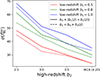Fig. 4. Forecasted error on $f_{\mathrm{NL}}^{\mathrm{loc}}$ as a function of the high-redshift bias prescription ${\overline{b}}_2(z)$. Solid lines correspond to a full rescaling of the galaxy bias by b0 in Eq. (18). In contrast, dashed lines correspond to rescaling only the high-redshift population bias by b0 in Eq. (20).

6.1.4. Impact of the outlier fraction

We model the Payerne et al. (2025) redshift distribution as in Eq. (17), depending on the outlier fraction at z < 1, (cf. Section 6.1.4). This modeling allows us to account for the effect of low-redshift outliers and to assess how $f_{\mathrm{NL}}^{\mathrm{loc}}$ constraints are impacted when the sample is more or less contaminated. We vary f_out following Mill et al. (2025), considering the values {0, 0.1, 0.2, 0.3, 0.4, 0.5} while keeping the total LBG number density fixed. Maintaining the same number density ensures that the Random Forest required density budget is unchanged, but with varying efficiency in selecting high-redshift LBGs. For f_out = 0 (no contamination), we obtain the tightest constraint, $\sigma (f_{\mathrm{NL}}^{\mathrm{loc}})=16$. As f_out increases from 0.1 to 0.5, the precision degrades approximately linearly, with $\sigma (f_{\mathrm{NL}}^{\mathrm{loc}})$ increasing to $\sigma (f_{\mathrm{NL}}^{\mathrm{loc}})=120$.

For the two alternative Random Forest selections based on UNIONS-like and LSSTY4-like photometry yielding 1100 LBG per square degrees, namely UNIONSlike_RF_u180s and LSSTY4like_RF_u2x180s (presented in Section 3), we obtain $\sigma (f_{\mathrm{NL}}^{\mathrm{loc}})=36$ and $\sigma (f_{\mathrm{NL}}^{\mathrm{loc}})=28$, respectively. Still in the context of modifying the outlier fraction, we can assess the precision on $f_{\mathrm{NL}}^{\mathrm{loc}}$ for a DESI-II-like sample, i.e., when the outliers can be removed by spectroscopic redshift confirmation. Considering the z > 2 part of the sample only (and modifying the LBG density accordingly, i.e., 800 LBG per square degree) we get that $\sigma (f_{\mathrm{NL}}^{\mathrm{loc}})=15$. When accounting for the DESI spectroscopic redshift efficiency for 2-hour exposure (resp. 4-hour), we get $\sigma (f_{\mathrm{NL}}^{\mathrm{loc}})=22$ (resp. $\sigma (f_{\mathrm{NL}}^{\mathrm{loc}})=20$). We observe that a higher precision on $f_{\mathrm{NL}}^{\mathrm{loc}}$ can be achieved by removing outliers, which motivates enhanced sample selection from photometric datasets, and their spectroscopic follow-up, even if the current DESI spectroscopic redshift efficiency removes most of the z < 2 targets.

6.1.5. Impact of the redshift distribution uncertainty

Here we explore the impact of the n(z) uncertainty on the PNG constraints, with two models described in Section 4.3. For the first, we consider random samples ${\widehat{n}}_k\sim \mathcal{N}(n(z),\sigma (z))$, where σ(z) is taken to be 0.2 n(z). In the second, we generate samples ${\widehat{n}}_k$, with the so-called shift-and-stretch method: we shift the high-redshift part of the n(z) by a random factor Δz ∼ 𝒩(0, 0.1), and stretch it by a random factor 1 + α ∼ 𝒩(1, 0.1). To derive the error on $f_{\mathrm{NL}}^{\mathrm{loc}}$ accounting for the uncertainty on the n(z), we stack the chains once converged and compute the mean and variance from the stacked chains (as explained in Eq. (26)).

For the first model, considering fitting C_ℓ^κg-only, the standard deviation STD of $f_{\mathrm{NL}}^{\mathrm{loc}}$ and b₀ best-fits over the 50 MCMCs are STD$(f_{\mathrm{NL}}^{\mathrm{loc}})=6$ and STD(b₀) = 0.01, respectively. Marginal error on $f_{\mathrm{NL}}^{\mathrm{loc}}$ and b₀ are obtained after stacking the chains, and we get $\sigma (f_{\mathrm{NL}}^{\mathrm{loc}})\approx 35$, that we retrieve if we consider the approximation $\sigma (f_{\mathrm{NL}}^{\mathrm{loc}})=\sqrt{{\sigma }_{\mathrm{fid}}^2(f_{\mathrm{NL}}^{\mathrm{loc}})+{\mathrm{STD}}^2(f_{\mathrm{NL}}^{\mathrm{loc}})}$, and σ(b₀)≈0.08 similar to the fiducial fit, the effect of $f_{\mathrm{NL}}^{\mathrm{loc}}$ precision is really small.

Using shift and stretch, we find similar results, namely that the dispersion of $f_{\mathrm{NL}}^{\mathrm{loc}}$ over the 50 MCMCs is roughly STD$(f_{\mathrm{NL}}^{\mathrm{loc}})=6$, leading to very few differences on the $f_{\mathrm{NL}}^{\mathrm{loc}}$ precision when stacking chains and taking the marginal dispersion, i.e., $\sigma (f_{\mathrm{NL}}^{\mathrm{loc}})=35$. From this simple exercise, we tested the robustness of $f_{\mathrm{NL}}^{\mathrm{loc}}$ constraints when accounting for the galaxy sample redshift uncertainty. We find that the effect is rather small for a well-calibrated n(z).

6.2. From early UNIONS LBG samples

In this section, we go beyond our idealistic LBG samples obtained in Payerne et al. (2025) to explore how $f_{\mathrm{NL}}^{\mathrm{loc}}$ forecasts can be conducted using LBG selection on the early UNIONS multiband data. We first discuss the selection we use on the GAaP multiband catalog, and then we discuss the methodology to infer the LBG redshift distribution.

6.2.1. CLAUDS+HSC-calibrated n(z)

From the CLAUDS+HSC-calibrated redshift distribution presented in Figure 1 (right panel) and the lensing magnification bias for this sample, we forecast a precision of $\sigma (f_{\mathrm{NL}}^{\mathrm{loc}})=20$ when adopting the Wilson et al. (2017) bias model. This result is slightly better than that of the baseline photometric sample from Payerne et al. (2025), which contains a more significant fraction of low-redshift outliers. In contrast, the UNIONS selection includes a higher number of galaxies in the redshift range 1.5 < z < 2, where the CMB lensing kernel peaks. Additionally, the UNIONS sample benefits from a higher galaxy density (increasing from 1100 to 1400 deg⁻²), a lower magnification bias, and a higher mean bias, corresponding to a deeper r-band limit magnitude (24.2 vs. 24.3). The usable area for the forecast is also extended to the full UNIONS footprint, since the selection relies solely on ugr magnitudes. After convolving the redshift distribution with the DESI redshift reconstruction efficiency for 2-hour (resp. 4-hour) spectroscopic exposures–and adjusting for the corresponding number densities–we obtain $\sigma (f_{\mathrm{NL}}^{\mathrm{loc}})=24$ (resp. $\sigma (f_{\mathrm{NL}}^{\mathrm{loc}})=23$), assuming only the UNIONS North Galactic Cap (NGC) footprint that DESI-II could realistically survey. The significant reduction in LBG number density for the DESI-II spectroscopic follow-up with 2-hours and 4-hours exposure time (down to 140 and 170 deg⁻²) arises from the higher proportion of UNIONS-LBGs that lie below z < 2 in the UNIONS selection compared to the selection in Payerne et al. (2025) peaking at z ≈ 3 (down to 500 and 590 deg⁻² from 1100 deg⁻² initially).

6.2.2. From clustering-redshifts with DESI DR1 data

In this section, we evaluate the degradation of the PNG constraints, using the clustering-redshift estimates of the LBG large-scale bias and redshift distribution (see Section 4.4). First, we fix bn to the measured b_LBGn_LBG with clustering redshifts, with corresponding b_eff = 1.5, leaving $f_{\mathrm{NL}}^{\mathrm{loc}}$ to be the only free parameter of the fit. For this setup, we obtain a fiducial uncertainty of $\sigma (f_{\mathrm{NL}}^{\mathrm{loc}})=57$ (without accounting for uncertainties in the clustering-redshift b(z)n(z) distribution), as the lower effective bias naturally reduces the constraining power. Then, we use the redshift-dependent bias model in Eq. (15), with a fixed rescaling factor ${\overline{b}}_0$ in Eq. (22). From this model, we obtain $\sigma (f_{\mathrm{NL}}^{\mathrm{loc}})=55$, quite similar to the late results obtained neglecting the bias redshift evolution through b_eff. From these results (still not accounting for the clustering-redshift uncertainties), we see that the previous result $\sigma (f_{\mathrm{NL}}^{\mathrm{loc}})=20$ assumes a high-bias, high-purity sample that is not currently supported by the clustering-redshift measurement.

To assess the impact of the uncertainty of the clustering-redshifts distribution, we generate random realizations $\widehat{\mathit{bn}}(z)\sim \mathcal{N}(b_{\mathrm{LBG}}{n}_{\mathrm{LBG}}(z),{\sigma }_{\mathrm{CZ}}(z))$, and ensure that $\widehat{\mathit{bn}}(z)$ remains positive. For each realization, we compute an effective bias ${\widehat{b}}_{\mathrm{eff}}$ as the redshift-integrated value of $\widehat{\mathit{bn}}(z)$. The fiducial data vector is obtained using the reference b_LBGn_LBG(z) and b_eff in Eq. (21), and 50 MCMC realizations are performed, accounting for the sampled $\widehat{\mathit{bn}}(z)$ and ${\widehat{b}}_{\mathrm{eff}}$ as input for the C_ℓ^κg modeling.

From this, the marginal uncertainty reaches $\sigma (f_{\mathrm{NL}}^{\mathrm{loc}})=134$ when stacking all converged chains. This corresponds to roughly a factor-of-two increase compared to the idealized case, reflecting a reduction in the forecasting power of the cross-correlation power spectrum. Importantly, this degradation is driven not by the dispersion in n(z) itself, but by the effective bias b_eff, which is closely linked to the constraining power on $f_{\mathrm{NL}}^{\mathrm{loc}}$–higher bias naturally leads to a better signal-to-noise ratio. Repeating the analysis with the error bars of the inferred clustering-redshift distribution reduced by a factor of $\sqrt{3}$–corresponding to the expected improvement in clustering-redshift precision with upcoming DESI DR3 data–reduces the uncertainty to $\sigma (f_{\mathrm{NL}}^{\mathrm{loc}})\approx 105$, highlighting the strong potential for improved clustering-redshift calibration with next-generation spectroscopic data.

Then we use the redshift-dependent bias model in Eq. (15), and we propagate uncertainties on the clustering-redshift distribution via $\widehat{\mathit{bn}}(z)\sim \mathcal{N}(b_{\mathrm{LBG}}{n}_{\mathrm{LBG}}(z),{\sigma }_{\mathrm{CZ}}(z))$ and ${\widehat{b}}_0$ to be the redshift integral of each $\widehat{\mathit{bn}}(z)/b_{\mathrm{W}19}(z)$. From this model, we obtain $\sigma (f_{\mathrm{NL}}^{\mathrm{loc}})=147$ when including DESI DR1 uncertainties, and $\sigma (f_{\mathrm{NL}}^{\mathrm{loc}})=120$ when assuming DESI DR3 performance. We can see that the more sophisticated model is not associated with an increase in the uncertainty in the fixed case, and creates a 15% degradation accounting for uncertainties. Thus, reducing the uncertainties associated with the clustering redshift measurements is the main limitation of this method.

This framework offers a promising avenue for combining clustering-redshift information with realistic bias modeling, representing an important step toward fully data-driven constraints on primordial non-Gaussianity. Even though current uncertainties remain significant and are the major contribution to the uncertainty on $f_{\mathrm{NL}}^{\mathrm{loc}}$, this exploratory analysis demonstrates the feasibility of applying clustering-redshift methods to LBG samples over such a wide redshift range, by combining the analysis of multiple DESI tracers.

Table A.1 lists the forecasted precision on $f_{\mathrm{NL}}^{\mathrm{loc}}$ and b₀ for the various analysis cases we explore in Sect. 6.2. To help isolate the gains due to sample properties versus simple volume expansion from the ugriz (Section 6.1) and ugr footprint (Section 6.2), we also rescaled the constraints in the summary table by the square root of the ratio between the footprints (a factor of 1.13).

7. Summary and conclusions

In this work, we investigated how effectively UNIONS-selected LBGs can constrain local primordial non-Gaussianities, quantified by the parameter $f_{\mathrm{NL}}^{\mathrm{loc}}$. When measured from large-scale structure, $f_{\mathrm{NL}}^{\mathrm{loc}}$ is intrinsically degenerate with the galaxy bias, represented here by b₀, and both parameters are jointly fitted throughout this study.

Using an idealized LBG sample from Payerne et al. (2025) identified from broadband ugriz bands using a Random Forest algorithm, peaking at z = 2 and with a surface density of 1100 deg⁻², we found that the scales most relevant for $f_{\mathrm{NL}}^{\mathrm{loc}}$ measurement (ℓ = 5 − 200) are dominated by cosmic variance. Consequently, expanding the survey area–and therefore increasing the number of available modes–directly enhances the precision on $f_{\mathrm{NL}}^{\mathrm{loc}}$ derived from the LBG angular power spectrum. In contrast, the cross-correlation between the LBG distribution and the Planck CMB lensing map remains limited by the noise of the latter. For our fiducial model, we obtained $\sigma (f_{\mathrm{NL}}^{\mathrm{loc}})=34$, with a 9% uncertainty in the recovered galaxy bias, assuming the universality relation b_ϕ = 2δ_c(b − p) with p_Φ = 1. However, the accuracy could be improved if the parameter p is lower than unity–an aspect that can be further investigated using cosmological simulations. By introducing a more complex, two-population bias model, we found that it degraded the precision to $\sigma (f_{\mathrm{NL}}^{\mathrm{loc}})=44$. We also examined the impact of photometric outliers on $f_{\mathrm{NL}}^{\mathrm{loc}}$ constraints. Tests using more realistic UNIONS-like datasets, from coadded U-band exposure on COSMOS, confirmed the strong role of outliers in degrading $f_{\mathrm{NL}}^{\mathrm{loc}}$ constraints. Considering UNIONS as an option for DESI-II target selection naturally removes outliers below z = 2.2 through spectroscopic confirmation, yielding a precision of $\sigma (f_{\mathrm{NL}}^{\mathrm{loc}})=22$, accounting for DESI redshift efficiency. This clearly demonstrated that reducing the fraction of outliers – even at the cost of a lower LBG density – significantly enhances the accuracy of $f_{\mathrm{NL}}^{\mathrm{loc}}$ measurements. We further assessed the robustness of our forecasts to uncertainties in the underlying redshift distribution n(z). Randomizing n(z) at the 20% level or applying a shift-and-stretch modification impacted $\sigma (f_{\mathrm{NL}}^{\mathrm{loc}})$ by less than 1%, confirming the stability of our results against such variations.

Finally, leveraging early UNIONS data, we tested LBG selection on real observations. The LBG sample obtained on XMM was matched to the deep photometric catalog from CLAUDS+HSC to assess their n(z), from which we found $\sigma (f_{\mathrm{NL}}^{\mathrm{loc}})=20$ with the Wilson & White (2019) bias model, leveraging the wider UNIONS footprint (the UNIONS selection relies only on ugr, not ugriz as in Payerne et al. 2025), a larger linear bias (due to the lower magnitude limit) and a broader coverage of the CMB lensing kernel. In the context of DESI-II, spectroscopic follow-up would allow us to reach the high-redshift end of the distribution with no uncertainties on the redshift distribution, providing $\sigma (f_{\mathrm{NL}}^{\mathrm{loc}})=24$. We then used the clustering-redshift technique (Ménard et al. 2013; d’Assignies et al. 2025b) to assess the redshift distribution of the UNIONS photometrically selected LBGs by cross-correlating them with DESI DR1 tracers over the wide range 0 < z < 3.5. We found good agreement with the CLAUDS+HSC calibrated distribution, demonstrating the application of clustering redshifts to such an extensive redshift interval for LBGs. However, when accounting for uncertainties in the clustering-redshift b(z)n(z) distribution, the constraint broadens to $\sigma (f_{\mathrm{NL}}^{\mathrm{loc}})=134$, yet is expected to improve significantly to $\sigma (f_{\mathrm{NL}}^{\mathrm{loc}})=105$ with DESI DR3 data. Overall, these exploratory results highlight the promise of the clustering-redshift method as an independent method to validate the recovered photometric redshift distribution up to z > 2, without relying on deep photometric catalog or spectroscopic follow-ups.

Acknowledgments

The authors thank the anonymous reviewer for their insightful comments and suggestions. We thank David Alonso for his help in using the Core Cosmology Library (CCL, Chisari et al. 2019) and NaMaster (Alonso et al. 2019). C. P. and C. Y. acknowledge support from grant ANR-22-CE31-0009 for the HZ-3D-MAP project and from grant ANR-22-CE92-0037 for the DESI-Lya project. W. d’A. acknowledges support from the MICINN projects PID2019-111317GB-C32, PID2022-141079NB-C32, as well as predoctoral program AGAUR-FI ajuts (2024 FI-1 00692) Joan Oró. IFAE is partially funded by the CERCA program of the Generalitat de Catalunya.

References

Appendix A: Summary of $f_{\mathrm{NL}}^{\mathrm{loc}}$ forecasts

We present in Table A.1 a summary of the different forecast results on $f_{\mathrm{NL}}^{\mathrm{loc}}$ and b₀ (when considered, only the fractional error is reported in this table) that we conducted in this paper. Results are sorted by paper sections.

Appendix B: Scales probed by the LBG redshift distributions

In this appendix, we examine the comoving scales probed by the various LBG samples used in this work. The default angular multipole range is ℓ ∈ [5, 300], which we convert to comoving wavenumbers via $k(z)=\frac{\ell +1/2}{\chi (z)}$, where χ(z) is the comoving distance at redshift z. Fixing the minimum and maximum values of ℓ restricts the k-range to the region between the two blue lines shown in Figure B.1. We now examine the k − z regions spanned by the UNIONS-like RF selection from Payerne et al. (2025) (left panel of Figure 1). We draw redshift samples according to n(z)² (in red), corresponding to the LBG redshift distribution kernel, which peaks at z ∼ 3. The high-redshift tail probes scales k ≲ 0.05 h Mpc⁻¹, while the largest accessible scales are limited by the survey size at z = 3 with ℓ = 5, corresponding to k ≳ 10⁻³ h Mpc⁻¹. The RF UNIONS-like distribution also includes low-redshift outliers (z < 0.5), which primarily probe non-linear scales located above the blue dashed line in Figure B.1. We define the maximum wavenumber k_max(z) for which the linear matter power spectrum remains valid as k_max(z) = max{k | Δ²(k,z) < 0.2}, with

$$\begin{array}{c}\hfill {\mathrm{\Delta }}^2(k,z)=\frac{k^{3}P(k,z)}{2{\pi }^2},\end{array}$$(B.1)

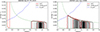Fig. B.1. Wavelength k − z plane. The region between the two green lines corresponds to all possible scales probed by the LBG samples. The area above the dashed blue line indicates non-linear scales. Left: The red (black) distribution shows the 1-2σ weighted k − z map following n(z)2 (n(z)Wκ(z), respectively) of the RF UNIONS-like selection from Payerne et al. (2025). Right: Same as the left plot, but for the UNIONS color-cut LBG selection.

where P(k, z) is the linear matter power spectrum evaluated at scale factor a = 1/(1 + z). The mode sensitivity when cross-correlating with CMB lensing – by drawing redshift samples according to n(z)W_κ(z) – represented in black in the left panel of Figure B.1, significantly reduces the importance of z < 0.5 objects, such as all scales probed are highly linear. For the UNIONS color-cut distribution, which probes somewhat smaller redshifts (right panel of Figure B.1), the minimum scale accessed by the high-redshift portion of the distribution (LBG redshift kernel only) is smaller than for the UNIONS-like RF selection, with k ≲ 0.075 h Mpc⁻¹. Overall, for the high-redshift portion of the LBG distributions considered in this work, the typical comoving wavenumber range is k ∈ [10⁻³, 0.075] h Mpc⁻¹. The low-redshift outliers probe smaller scales, but they constitute a much smaller fraction of the sample. When cross-correlating with CMB lensing, the scales probed are roughly the same, with a slightly higher sensitivity to high redshifts.

Appendix C: Magnification bias

In Figure C.1, we show the calculation of the magnification bias

$$\begin{array}{c}\hfill s(m_{\lim })=\frac{d{log}_{10}N(<m_{\lim },z)}{\mathit{dm}},\end{array}$$(C.1)

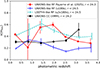Fig. C.1. Magnification bias in several redshift intervals for the different LBG samples we use in this work.

for different redshift intervals (the redshift intervals are obtained using LePhare photometric redshifts on COSMOS and XMM). For the different samples, we see some redshift variation over the redshift range. We adopt a conservative approach by using the mean value over the redshift range 0 < z < 4.

Appendix D: Investigating tomographic LBG samples

In this appendix, we consider the UNIONS-like RF sample presented in Section 3, with a surface density of 1100 deg⁻² over the full redshift range 0 < z < 4. For the tomographic approach, we split the sample into three redshift bins with edges at z = 1.5, 2.6, 2.9, and 3.5, such that the corresponding number density in each bin is approximately 300 deg⁻². Figure D.1 (top panel) shows the per-ℓ quantity C_ℓ^gg × n_gal for the three tomographic bins, as well as for a single bin that includes all LBGs contained in the three bins. On scales 10 < ℓ < 300, the LBG-only angular power spectrum remains cosmic-variance dominated. The bottom panel shows the signal-to-noise ratio of the C_ℓ^κg signal for the three bins and the single bin approach, demonstrating that it is significantly degraded when adopting a tomographic approach.

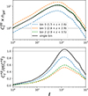Fig. D.1. Top: Ratio of the predicted angular power spectrum of the LBG population, split into three tomographic redshift bins (together with the single-bin prediction), to the corresponding galaxy shot noise. Bottom: Corresponding signal-to-noise ratio of the angular cross-correlation power spectrum between the LBG tomographic samples and CMB lensing.

Appendix E: Degrading deep photometric datasets

E.1. CLAUDS U-band forced photometry using HSC g-band detection position

The resulting U-band PSF depth distribution, obtained by performing forced photometry in the g-band on the U-band CLAUDS images (with exposure times of t_exp = 180 s and t_exp = 2 × 180 s, respectively), is shown in Figure E.1, together with two additional runs of 3 × 180 s and 600 s (the default t_exp of for the released CLAUDS catalog available at https://www.clauds.net), respectively. From the plot, the higher t_exp, the higher the mean U-band PSF depth we get. For t_exp = 180 s and t_exp = 2 × 180 s, we get a mean PSF depth of 24.6 and 25. Let us note that this enables us to have UNIONS-like data in the U-band, not in the other bands (griz). This is explained in the next section.

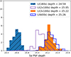Fig. E.1. 5σ PSF depth for U-band data, obtained by forced photometry at the HSC g-band detection position. The different histograms are obtained by considering different texp for the CLAUDS U-band images.

E.2. Artificially degrading a deeper photometric dataset to shallower depths

For the other bands (griz), we follow the method presented in Payerne et al. (2025). The shallow magnitude m_shallow is obtained from the deep magnitude m_deep (from the HSC catalog) by adding noise in flux space corresponding to a shallower limiting depth. The deep flux is first computed as

$$\begin{array}{c}\hfill f_{\mathrm{deep}}={10}^{-0.4(m_{\mathrm{deep}}-22.5)}.\end{array}$$(E.1)

The shallow flux is obtained by adding a Gaussian random deviate,

$$\begin{array}{c}\hfill f_{\mathrm{shallow}}\sim \mathcal{N}(f_{\mathrm{deep}},{\sigma }_{f,\mathrm{add}}^2).\end{array}$$(E.2)

where an additional flux uncertainty σ_f,add is introduced,

$$\begin{array}{c}\hfill {\sigma }_{f,\mathrm{add}}=f_{\mathrm{deep}}\frac{{\sigma }_{m,\mathrm{add}}}{2.5/ln10}.\end{array}$$(E.3)

The corresponding shallow magnitude is

$$\begin{array}{c}\hfill m_{\mathrm{shallow}}=22.5-2.5{log}_{10}\left(f_{\mathrm{shallow}}\right).\end{array}$$(E.4)

The additional magnitude uncertainty σ_m,add is defined such that the total magnitude error matches that expected at the shallower depth,

$$\begin{array}{c}\hfill {\sigma }_{m,\mathrm{add}}=\sqrt{{\sigma }_m^2(m_{\mathrm{deep}},m_{\mathrm{shallow}\mathrm{depth}})-{\sigma }_m^2(m_{\mathrm{deep}},m_{\mathrm{deep}\mathrm{depth}})},\end{array}$$(E.5)

with

$$\begin{array}{c}\hfill {\sigma }_m(m,\mathrm{depth})=\frac{2.5}{ln10}\frac{1}{N_{\sigma }}{10}^{0.4(m-\mathrm{depth})},\end{array}$$(E.6)

where N_σ = 5. An illustration of this procedure is shown in Figure E.2 for the degradation of HSC magnitudes measured in the r band. The deep r-band magnitude distribution, shown in blue, corresponds to a 5σ depth of r = 26.6. After applying the artificial degradation, the resulting shallow magnitude distribution is shown in magenta and corresponds to a simulated 5σ depth of r = 25.5. Reaching a shallower depth also implies a reduced number of detected objects. To explore how detection efficiency modifies the histograms, we model this effect by applying a random selection of sources based on their probability of detection in the shallower survey. Assuming Gaussian flux uncertainties and a detection threshold of N_σ = 3, the detection probability for an object of magnitude m is given by

$$\begin{array}{c}\hfill P_{\det }(m_{\mathrm{deep}})=\frac{1}{2}[1-\mathrm{erf}\left(\frac{N_{\sigma }{\sigma }_f-f_{\mathrm{deep}}}{\sqrt{2}{\sigma }_f}\right)],\end{array}$$(E.7)

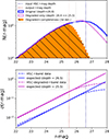Fig. E.2. Top: Histogram of r-band magnitudes before (blue) and after (magenta) applying the artificial degradation procedure. The orange histogram shows the magnitude distribution after applying the detection efficiency of the shallower survey. Bottom: r-band magnitude uncertainty as a function of magnitude before (blue) and after (magenta) applying the artificial degradation procedure.

where σ_f = f(m_{shallow depth})/5. The resulting magnitude distribution after applying this completeness selection is shown in orange in Figure E.2 (upper panel), and exhibits the same turnover at the limiting depth as the deep sample. For the r-band cut we use in this work (of about 24.2 to 24.5), we are not sensitive to this photometric detection efficiency effect. Finally, the bottom plot show the magnitude error σ_m,deep and σ_m,shallow given by

$$\begin{array}{c}\hfill {\sigma }_{m,\mathrm{shallow}}=\sqrt{{\sigma }_{m,\mathrm{deep}}^2+{\sigma }_{m,\mathrm{add}}^2}\end{array}$$(E.8)

with respect to magnitude for the deep and shallow r-band catalog, matching their expected value in Eq. (E.6). We note that a more sophisticated error model exists to describe the turnover of the magnitude error at the magnitude depth (see Figure E.2, lower panel), as explained in Section 3.2.4 of Hildebrandt et al. (2010), used in Wilson & White (2019) for degradation.

All Tables

All Figures

Fig. 1. Left: Photometric redshift distributions of the photometric LBG samples UNIONSlike_RF in red (the convolution of the UNIONSlike_RF distribution with the DESI spectroscopic efficiency is shown in dashed and dotted lines, they have not been normalized to show the impact at z ∼ 2.5). The distribution of the samples UNIONSlike_RF_u180s, and LSSTY4like_RF_u2x180s are shown in blue and dashed cyan lines. Right: Photometric redshift distributions of the UNIONS LBG samples UNIONS_colorcut and UNIONS_PZcut in the XMM field. The sample selected with the hybrid method à-la SOM is shown for illustration. We also show the quantity nb (the product between the large-scale bias and the normalized redshift distribution) resulting from our clustering-redshift calibration methods.

In the text

	Fig. 2. Top panel shows the angular power spectra Cℓgg, Cℓκg, and Cℓκκ (solid lines) for the baseline sample. The cosmological-only contribution is shown as dashed lines, while the noise contribution is shown as dotted lines. Bottom panel shows the signal-to-noise ratio, defined as the ratio of the cosmological-only term to the noise, for Cℓgg and Cℓκκ.
In the text

Fig. 3. Left: Posterior distribution of the parameters $f_{\mathrm{NL}}^{\mathrm{loc}}$ and the large-scale linear bias (expressed in terms of relative error). Right: Forecasted error on $f_{\mathrm{NL}}^{\mathrm{loc}}$ as a function of the lower multipole cut ℓmin. Solid lines show constraints using only $C_{\ell }^{\kappa g}(\ell >{\ell }_{\min })$, while dashed lines correspond to the combination of $C_{\ell }^{\kappa g}$ and $C_{\ell }^{\mathit{gg}}(\ell >{\ell }_{\min })$. Different colors indicate different LBG number densities: 800, 1100, and 2000 LBGs per deg2.

In the text

	Fig. 4. Forecasted error on $f_{\mathrm{NL}}^{\mathrm{loc}}$ as a function of the high-redshift bias prescription ${\overline{b}}_2(z)$. Solid lines correspond to a full rescaling of the galaxy bias by b0 in Eq. (18). In contrast, dashed lines correspond to rescaling only the high-redshift population bias by b0 in Eq. (20).
In the text

Fig. B.1. Wavelength k − z plane. The region between the two green lines corresponds to all possible scales probed by the LBG samples. The area above the dashed blue line indicates non-linear scales. Left: The red (black) distribution shows the 1-2σ weighted k − z map following n(z)2 (n(z)Wκ(z), respectively) of the RF UNIONS-like selection from Payerne et al. (2025). Right: Same as the left plot, but for the UNIONS color-cut LBG selection.

In the text

	Fig. C.1. Magnification bias in several redshift intervals for the different LBG samples we use in this work.
In the text

	Fig. D.1. Top: Ratio of the predicted angular power spectrum of the LBG population, split into three tomographic redshift bins (together with the single-bin prediction), to the corresponding galaxy shot noise. Bottom: Corresponding signal-to-noise ratio of the angular cross-correlation power spectrum between the LBG tomographic samples and CMB lensing.
In the text

	Fig. E.1. 5σ PSF depth for U-band data, obtained by forced photometry at the HSC g-band detection position. The different histograms are obtained by considering different texp for the CLAUDS U-band images.
In the text

	Fig. E.2. Top: Histogram of r-band magnitudes before (blue) and after (magenta) applying the artificial degradation procedure. The orange histogram shows the magnitude distribution after applying the detection efficiency of the shallower survey. Bottom: r-band magnitude uncertainty as a function of magnitude before (blue) and after (magenta) applying the artificial degradation procedure.
In the text

References

- Aihara, H., AlSayyad, Y., Ando, M., et al. 2022, PASJ, 74, 247 [NASA ADS] [CrossRef] [Google Scholar]
- Alonso, D., Sanchez, J., Slosar, A., & LSST Dark Energy Science Collaboration 2019, MNRAS, 484, 4127 [NASA ADS] [CrossRef] [Google Scholar]
- Anbajagane, D., Chang, C., Lee, H., & Gatti, M. 2024, JCAP, 2024, 062 [Google Scholar]
- Barreira, A. 2020, JCAP, 2020, 031 [CrossRef] [Google Scholar]
- Barreira, A., Cabass, G., Schmidt, F., Pillepich, A., & Nelson, D. 2020, JCAP, 2020, 013 [NASA ADS] [CrossRef] [Google Scholar]
- Benítez, N. 2011, Astrophysics Source Code Library [record ascl:1108.011] [Google Scholar]
- Bernstein, G., Assignies Doumerg, W., Troxel, M. A., et al. 2025, ArXiv e-prints [arXiv:2506.00758] [Google Scholar]
- Besuner, R., Dey, A., Drlica-Wagner, A., et al. 2025, ArXiv e-prints [arXiv:2503.07923] [Google Scholar]
- Brown, M. L., Castro, P. G., & Taylor, A. N. 2005, MNRAS, 360, 1262 [NASA ADS] [CrossRef] [Google Scholar]
- Busca, N., & Balland, C. 2018, ArXiv e-prints [arXiv:1808.09955] [Google Scholar]
- Cagliari, M. S., Castorina, E., Bonici, M., & Bianchi, D. 2024, JCAP, 2024, 036 [Google Scholar]
- Carron, J. 2013, A&A, 551, A88 [NASA ADS] [CrossRef] [EDP Sciences] [Google Scholar]
- Carron, J., Mirmelstein, M., & Lewis, A. 2022, JCAP, 2022, 039 [CrossRef] [Google Scholar]
- Challinor, A., & Lewis, A. 2011, Phys. Rev. D, 84, 043516 [NASA ADS] [CrossRef] [Google Scholar]
- Chambers, K. C., Magnier, E. A., Metcalfe, N., et al. 2016, ArXiv e-prints [arXiv:1612.05560] [Google Scholar]
- Chaussidon, E., Yèche, C., Palanque-Delabrouille, N., et al. 2022, MNRAS, 509, 3904 [Google Scholar]
- Chaussidon, E., Yèche, C., de Mattia, A., et al. 2025, JCAP, 2025, 029 [Google Scholar]
- Chiarenza, S., Krolewski, A., Bonici, M., et al. 2025, ArXiv e-prints [arXiv:2512.17865] [Google Scholar]
- Chisari, N. E., Alonso, D., Krause, E., et al. 2019, ApJS, 242, 2 [Google Scholar]
- Choi, A., Heymans, C., Blake, C., et al. 2016, MNRAS, 463, 3737 [Google Scholar]
- Choppin de Janvry, J., Gontcho, S. G. A., Seljak, U., et al. 2025, ArXiv e-prints [arXiv:2511.18133] [Google Scholar]
- Crenshaw, J. F., Leistedt, B., Graham, M. L., et al. 2025, ApJS, 281, 54 [Google Scholar]
- CSST Collaboration (Gong, Y., et al.) 2026, Sci. China Phys. Mech. Astron., 69, 239501 [Google Scholar]
- Dalal, N., Doré, O., Huterer, D., & Shirokov, A. 2008, Phys. Rev. D, 77, 123514 [CrossRef] [Google Scholar]
- d’Assignies, D. W., Zhao, C., Yu, J., & Kneib, J. P. 2023, MNRAS, 521, 3648 [Google Scholar]
- d’Assignies, W., Bernstein, G. M., Yin, B., et al. 2025a, ArXiv e-prints [arXiv:2510.23565] [Google Scholar]
- d’Assignies, W., Manera, M., Padilla, C., et al. 2025b, A&A, 702, A155 [Google Scholar]
- Desjacques, V., & Seljak, U. 2010, Class. Quant. Grav., 27, 124011 [Google Scholar]
- Desjacques, V., Jeong, D., & Schmidt, F. 2018, Phys. Rep., 733, 1 [Google Scholar]
- Desprez, G., Picouet, V., Moutard, T., et al. 2023, A&A, 670, A82 [NASA ADS] [CrossRef] [EDP Sciences] [Google Scholar]
- Doux, C., Penna-Lima, M., Vitenti, S. D. P., et al. 2018, MNRAS, 480, 5386 [Google Scholar]
- Elvin-Poole, J., MacCrann, N., Everett, S., et al. 2023, MNRAS, 523, 3649 [NASA ADS] [CrossRef] [Google Scholar]
- Euclid Collaboration (Lepori, F., et al.) 2022, A&A, 662, A93 [NASA ADS] [CrossRef] [EDP Sciences] [Google Scholar]
- Fabbian, G., Alonso, D., Storey-Fisher, K., & Cornish, T. 2026, JCAP, 2026, 056 [Google Scholar]
- Foreman-Mackey, D., Hogg, D. W., Lang, D., & Goodman, J. 2013, PASP, 125, 306 [Google Scholar]
- Foucaud, S., McCracken, H. J., Le Fèvre, O., et al. 2003, A&A, 409, 835 [Google Scholar]
- Giannini, G., Alarcon, A., d’Assignies, W., et al. 2025, ArXiv e-prints [arXiv:2509.07964] [Google Scholar]
- Giavalisco, M., Dickinson, M., Ferguson, H. C., et al. 2004, ApJ, 600, L103 [NASA ADS] [CrossRef] [Google Scholar]
- Guy, J., Bailey, S., Kremin, A., et al. 2023, AJ, 165, 144 [NASA ADS] [CrossRef] [Google Scholar]
- Gwyn, S., McConnachie, A. W., Cuillandre, J.-C., et al. 2025, AJ, 170, 324 [Google Scholar]
- Harikane, Y., Ono, Y., Ouchi, M., et al. 2022, ApJS, 259, 20 [NASA ADS] [CrossRef] [Google Scholar]
- Harikane, Y., Ouchi, M., Oguri, M., et al. 2023, ApJS, 265, 5 [NASA ADS] [CrossRef] [Google Scholar]
- Herrera-Alcantar, H. K., Armengaud, E., Yèche, C., et al. 2025, JCAP, 2025, 053 [Google Scholar]
- Hildebrandt, H., Pielorz, J., Erben, T., et al. 2009, A&A, 498, 725 [NASA ADS] [CrossRef] [EDP Sciences] [Google Scholar]
- Hildebrandt, H., Arnouts, S., Capak, P., et al. 2010, A&A, 523, A31 [NASA ADS] [CrossRef] [EDP Sciences] [Google Scholar]
- Hildebrandt, H., van den Busch, J. L., Wright, A. H., et al. 2021, A&A, 647, A124 [EDP Sciences] [Google Scholar]
- Ibata, R. A., McConnachie, A., Cuillandre, J.-C., et al. 2017, ApJ, 848, 128 [Google Scholar]
- Jarvis, M. 2015, Astrophysics Source Code Library [record ascl:1508.007] [Google Scholar]
- Jeong, D., Schmidt, F., & Sefusatti, E. 2011, Phys. Rev. D, 83, 123005 [Google Scholar]
- Krolewski, A., Percival, W. J., Ferraro, S., et al. 2024, JCAP, 2024, 021 [Google Scholar]
- Kuijken, K. 2008, A&A, 482, 1053 [NASA ADS] [CrossRef] [EDP Sciences] [Google Scholar]
- Kuijken, K., Heymans, C., Hildebrandt, H., et al. 2015, MNRAS, 454, 3500 [Google Scholar]
- Kuijken, K., Heymans, C., Dvornik, A., et al. 2019, A&A, 625, A2 [NASA ADS] [CrossRef] [EDP Sciences] [Google Scholar]
- Landy, S. D., & Szalay, A. S. 1993, ApJ, 412, 64 [Google Scholar]
- Lewis, A., & Challinor, A. 2006, Phys. Rep., 429, 1 [Google Scholar]
- Lima, M., Cunha, C. E., Oyaizu, H., et al. 2008, MNRAS, 390, 118 [Google Scholar]
- Limber, D. N. 1953, ApJ, 117, 134 [NASA ADS] [CrossRef] [Google Scholar]
- LSST Science Collaboration (Abell, P. A., et al.) 2009, ArXiv e-prints [arXiv:0912.0201] [Google Scholar]
- Mainieri, V., Anderson, R. I., Brinchmann, J., et al. 2024, ArXiv e-prints [arXiv:2403.05398] [Google Scholar]
- Malkan, M. A., Cohen, D. P., Maruyama, M., et al. 2017, ApJ, 850, 5 [NASA ADS] [CrossRef] [Google Scholar]
- Ménard, B., Scranton, R., Schmidt, S., et al. 2013, ArXiv e-prints [arXiv:1303.4722] [Google Scholar]
- Mergulhão, T., Rubira, H., Voivodic, R., & Abramo, L. R. 2022, JCAP, 2022, 021 [Google Scholar]
- Mill, C. M., Leonard, C. D., Rau, M. M., Uhlemann, C., & Joudaki, S. 2025, JCAP, 2025, 037 [Google Scholar]
- Miyatake, H., Harikane, Y., Ouchi, M., et al. 2022, Phys. Rev. Lett., 129, 061301 [NASA ADS] [CrossRef] [Google Scholar]
- Miyazaki, S., Komiyama, Y., Kawanomoto, S., et al. 2018, PASJ, 70, S1 [NASA ADS] [Google Scholar]
- Myles, J., Alarcon, A., Amon, A., et al. 2021, MNRAS, 505, 4249 [NASA ADS] [CrossRef] [Google Scholar]
- Okamoto, T., & Hu, W. 2003, Phys. Rev. D, 67, 083002 [NASA ADS] [CrossRef] [Google Scholar]
- Ono, Y., Ouchi, M., Harikane, Y., et al. 2018, PASP, 70, S10 [Google Scholar]
- Payerne, C., d’Assignies Doumerg, W., Yèche, C., et al. 2025, JCAP, 2025, 031 [Google Scholar]
- Petri, F., Leistedt, B., Mortlock, D. J., et al. 2026, MNRAS, 545, staf2115 [Google Scholar]
- Planck Collaboration IX. 2020, A&A, 641, A9 [Google Scholar]
- Reddy, N. A., Steidel, C. C., Pettini, M., et al. 2008, ApJS, 175, 48 [CrossRef] [Google Scholar]
- Rezaie, M., Ross, A. J., Seo, H.-J., et al. 2024, MNRAS, 532, 1902 [NASA ADS] [CrossRef] [Google Scholar]
- Ross, A. J., Aguilar, J., Ahlen, S., et al. 2025, JCAP, 2025, 125 [Google Scholar]
- Roster, W., Wright, A. H., Hildebrandt, H., et al. 2026, A&A, 707, A277 [Google Scholar]
- Ruhlmann-Kleider, V., Yèche, C., Magneville, C., et al. 2024, JCAP, 2024, 059 [Google Scholar]
- Sailer, N., Castorina, E., Ferraro, S., & White, M. 2021, JCAP, 2021, 049 [CrossRef] [Google Scholar]
- Sawicki, M., Arnouts, S., Huang, J., et al. 2019, MNRAS, 489, 5202 [NASA ADS] [Google Scholar]
- Schlegel, D. J., Ferraro, S., Aldering, G., et al. 2022, ArXiv e-prints [arXiv:2209.03585] [Google Scholar]
- Schmidt, S. J., Ménard, B., Scranton, R., Morrison, C., & McBride, C. K. 2013, MNRAS, 431, 3307 [Google Scholar]
- Schmittfull, M., & Seljak, U. 2018, Phys. Rev. D, 97, 123540 [NASA ADS] [CrossRef] [Google Scholar]
- Slosar, A., Hirata, C., Seljak, U., Ho, S., & Padmanabhan, N. 2008, JCAP, 2008, 031 [CrossRef] [Google Scholar]
- Steidel, C. C., Giavalisco, M., Pettini, M., Dickinson, M., & Adelberger, K. L. 1996, ApJ, 462, L17 [Google Scholar]
- Steidel, C. C., Adelberger, K. L., Giavalisco, M., Dickinson, M., & Pettini, M. 1999, ApJ, 519, 1 [NASA ADS] [CrossRef] [Google Scholar]
- Takahashi, R., Sato, M., Nishimichi, T., Taruya, A., & Oguri, M. 2012, ApJ, 761, 152 [Google Scholar]
- Wilson, M. J., & White, M. 2019, JCAP, 2019, 015 [Google Scholar]
- Wilson, M. J., Peacock, J. A., Taylor, A. N., & de la Torre, S. 2017, MNRAS, 464, 3121 [Google Scholar]
- Ye, I., Bull, P., Bowler, R. A. A., et al. 2025, MNRAS, 543, 3196 [Google Scholar]
- Yu, B., Knight, R. Z., Sherwin, B. D., et al. 2023, Phys. Rev. D, 107, 123522 [Google Scholar]
- Zhang, Y. H., Zuntz, J., Moskowitz, I., et al. 2025, MNRAS, submitted [arXiv:2508.20903] [Google Scholar]
Such as the fractional perturbation  , where κ is the projected matter density field along the line of sight, and
is the intrinsic clustering fractional perturbation.
i.e., the logarithmic slope of the cumulative number counts at the survey detection limit, where N(< m) is the number of objects brighter than magnitude m, and mlim is the survey flux limit.
Canada-France-Hawaii Telescope Large Area U-band Deep Survey, Sawicki et al. (2019).
Hyper Suprime-Camera, Aihara et al. (2022).
First, a convolutional neural network (CNN) derived from QuasarNET (Busca & Balland 2018) is applied to each DESI spectrum. A more precise LBG redshift is then obtained using the RedRock (RR) software (Guy et al. 2023) that uses the CNN output redshift as a prior and refines its measurement.
CFHTLS-Archive-Research Survey.
Great Optically Luminous Dropout Research Using Subaru HSC.
With typical bias bW19(z = 2.5, mlim = 24.2) = 4, bW19(z = 2.5, mlim = 24.3) = 3.8 and bW19(z = 2.5, mlim = 24.5) = 3.4.
Appendix A: Summary of  forecasts