


| Issue |
A&A
Volume 709, May 2026
|
|
|---|---|---|
| Article Number | A211 | |
| Number of page(s) | 16 | |
| Section | The Sun and the Heliosphere | |
| DOI | https://doi.org/10.1051/0004-6361/202558324 | |
| Published online | 19 May 2026 | |
Formation and rising phase of a flux rope through data-constrained simulations
1
Département d’Astrophysique/AIM, CEA/IRFU, CNRS/INSU, Univ. Paris-Saclay & Univ. de Paris, 91191 Gif-sur-Yvette, France
2
Statkraft AS, Lysaker, Norway
3
Institute of Theoretical Astrophysics, University of Oslo, P.O. Box 1029 Blindern, N-0315 Oslo, Norway
4
Rosseland Centre for Solar Physics, University of Oslo, P.O. Box 1029 Blindern, N-0315 Oslo, Norway
5
Department of Physics, University of Helsinki, P.O. Box 64, FI-00014, Helsinki, Finland
6
LIRA, Observatoire de Paris, Université PSL, Sorbonne Université, Paris Ciét, CY Cergy Paris Université, CNRS, 92190 Meudon, France
7
Instituto de Astrofisica de Canarias, E-38205 La Laguna, Tenerife, Spain
8
Departamento de Astrofisica, Universidad de La Laguna, E-38206 La Laguna, Tenerife, Spain
9
Heliophysics Science Division, NASA Goddard Space Flight Center, Greenbelt, MD 20771, USA
10
Department of Physics and Astronomy, George Mason University, Fairfax, VA 22030, USA
11
European Space Agency, ESTEC, Noordwijk, The Netherlands
12
Université Paris-Saclay, CNRS, Institut d’Astrophysique Spatiale, 91405 Orsay, France
★ Corresponding author: This email address is being protected from spambots. You need JavaScript enabled to view it.
Received:
30
November
2025
Accepted:
17
March
2026
Abstract
Context. Advances in data-constrained and data-driven simulations have shed light on the initiation of solar eruptions. These models incorporate observed photospheric magnetic fields. However, because we lack information about the magnetic field in the rest of the solar atmosphere, models rely on extrapolations that, in most cases, neglect the Lorentz force. Nevertheless, this force is present in the lower atmosphere and may play a key role in destabilising the equilibrium configuration and triggering eruptions.
Aims. This study seeks to understand and reproduce solar eruption SOL2014-12-18T21:41, which occurred in active region NOAA 12241 and was preceded by an M6.9 flare. We also investigate the effect of relaxing the initial force-free assumption.
Methods. The resistive and compressible magnetohydrodynamic simulation was initiated using a non-force-free magnetic field extrapolated from a photospheric vector magnetogram taken minutes before the flare. The simulation included a stratified atmosphere and non-ideal effects such as thermal conduction and radiative cooling.
Results. A flux rope forms and rises in the simulation and carries dense material away from the lower solar atmosphere. Its formation results from the non-zero Lorentz force acting on the initial sheared arcade, without assuming pre-existing flux ropes or photospheric driving motions. The flux rope is then deflected towards regions of low magnetic pressure, escaping from the domain at 350 km s−1 with approximately constant acceleration.
Conclusions. A robust numerical framework for modelling flaring active regions was applied to the eruption of NOAA AR 12241 as a case study, assuming a realistic non-force-free magnetic field near the flare onset. It exemplifies how an initial imbalance in the Lorentz force can successfully trigger a flux rope formation that later escapes from the simulation domain. It also enables comparison with real observations through the addition of a stratified atmosphere spanning from the photosphere to the corona.
Key words: magnetohydrodynamics (MHD) / Sun: atmosphere / Sun: flares / Sun: magnetic fields
© The Authors 2026
 Open Access article, published by EDP Sciences, under the terms of the Creative Commons Attribution License (https://creativecommons.org/licenses/by/4.0), which permits unrestricted use, distribution, and reproduction in any medium, provided the original work is properly cited.
This article is published in open access under the Subscribe to Open model. This email address is being protected from spambots. You need JavaScript enabled to view it. to support open access publication.
1. Introduction
Solar eruptions are one of the most frequently studied dynamical events in the solar atmosphere. These explosive events are usually associated with flares, coronal mass ejections (CMEs), and energetic particles. During flares, magnetic energies between 1028 and 1031 erg are released and converted into kinetic, thermal, and non-thermal energies (Shibata & Magara 2011; Fletcher et al. 2011; Benz 2017). As a consequence, they can lead to extreme-ultraviolet and X-ray radiation, particle acceleration, and material ejection (CMEs), all of which can dramatically affect space weather.
There are two main initiation categories of eruptions (Jiang 2024): one category is based on the ideal magnetohydrodynamic (MHD hereafter) instability of a pre-existing magnetic flux rope (Titov & Démoulin 1999; Titov et al. 2018), and the other category is based on reconnection of sheared field lines with or without a flux rope. Within the first category, two of the MHD instabilities are commonly considered: the kink instability (Hood & Priest 1979; Török et al. 2004; Ji et al. 2003), and the torus instability (Kliem & Török 2006). In their simplest form, these instabilities are triggered when the magnetic configuration exceeds a threshold, namely, of the total number of magnetic windings between the line-tied ends for the kink instability (Hood & Priest 1979), or the decay index with height of the external strapping magnetic field for the torus instability (Kliem & Török 2006). Regarding the second category, the reconnection-based models include, roughly speaking, the tether-cutting (Moore et al. 2001) and the breakout model (Antiochos et al. 1999). An example of the tether-cutting mechanism is the standard flare model (e.g. Carmichael 1964; Sturrock & Coppi 1965; Hirayama 1974; Kopp & Pneuman 1976; Janvier et al. 2014), in which there is a pre-existing magnetic flux rope.
Numerical simulations usually involve a combination of these ideal and reconnection processes together with triggering mechanisms at photospheric or chromospheric levels, such as shearing motions (Lynch et al. 2008; Pariat et al. 2010; Wyper et al. 2017; Joshi et al. 2024a), flux cancellation (Amari et al. 2003; Linker et al. 2003; Aulanier et al. 2010; Zuccarello et al. 2015), and flux emergence (Leake et al. 2010, 2014, 2022; MacTaggart & Haynes 2014).
In real events, the process is even more complex, and eruptions may not obey these idealised theoretical mechanisms. It remains unclear how solar eruptions are initiated, especially because we lack direct observational information about the magnetic field strength and orientation in the corona. In order to better understand the mechanisms that cause solar eruptions, data-based models constrained by photospheric observations have therefore been shown to be an appropriate path (we refer to the review papers of Inoue 2016; Jiang et al. 2022, for such data-based simulations). We can distinguish between data-constrained simulations in which the initial conditions are derived from observational data at the solar surface at a single time and data-driven simulations that use time-dependent boundary conditions derived from observational time series.
Data-constrained simulations focus on the eruption process and are generally initialised with close to unstable magnetic configurations extrapolated from vector magnetograms at a moment shortly before eruption onset. For example, using non-linear force-free extrapolations (NLFFF hereafter), several authors (Jiang et al. 2013; Amari et al. 2014; Yamasaki et al. 2022; Zhong et al. 2023) showed that in data-constrained simulations of active regions, eruptions are triggered by a torus instability, and that magnetic reconnection allows the full development of the instability by removing part of the line-tied connections. Another approach is to start from an initially stable magnetic configuration and trigger the eruption through photospheric motions, such as shearing and convergence (Inoue et al. 2018; Török et al. 2018), or flux emergence (Fan 2011, 2022; Muhamad et al. 2017; Inoue et al. 2025).
On the other hand, the bottom boundary conditions in fully data-driven MHD simulations are specified by the observables in the photosphere in a time-dependent way, covering from several hours to several days of the pre-eruption phase (Jiang et al. 2016; Wang et al. 2023; Chen et al. 2023; Guo et al. 2023). Since it is computationally expensive to simulate the long-term pre-eruption phase in full MHD, another option is to use the data-driven magnetofrictional technique (Cheung & DeRosa 2012; Gibb et al. 2014; Pomoell et al. 2019; Price et al. 2019, 2020; Kilpua et al. 2021) to simulate the process ahead of the eruption, and apply the full MHD modelling only to the eruption itself (Afanasyev et al. 2023; Daei et al. 2023; Guo et al. 2024). However, choosing an appropriate time step for switching from magnetofriction to MHD is non-trivial as the properties of the erupting system significantly depend on the chosen simulation frame for this transfer (Wagner et al. 2024b).
In all the data-driven or data-constrained simulations mentioned above, the coronal fields are numerically extrapolated from the photospheric magnetic distribution based on a force-free assumption, that is, no Lorentz force is exerted (Wheatland & Gilchrist 2013; Wiegelmann & Sakurai 2021). This is based on the hypothesis that the coronal magnetic fields evolve continuously driven by motions at the photosphere in a quasi-static way. Although simulations based on NLFFF extrapolations are capable of reproducing realistic dynamics, the magnetic field in the photosphere is generally not perfectly force-free (e.g. Schuck et al. 2022). Moreover, the force-free approximation is based on the assumption of negligible plasma-β, but this is only true in the transition region and low corona (Gary 2001). Since the extrapolations for the aforementioned models take their bottom boundary in the photospheric magnetic field below the chromosphere, where β ≥ 1, a non-force-free extrapolation approach should generally be more realistic.
Thus, we consider a non-force-free field (NFFF hereafter) extrapolation, prescribing the magnetic field at the photosphere with a vector magnetogram close to the onset of the flare. As the name suggests, this technique allows us to have a non-zero Lorentz force, which is a crucial point because during solar eruptions, the coronal magnetic field is far from equilibrium. The NFFF extrapolation relies on self-organised double-curl Beltrami fields (Bhattacharyya et al. 2007) satisfying the minimum dissipation rate principle (Bhattacharyya & Janaki 2004; Bhattacharyya et al. 2007; Hu & Dasgupta 2008). Comparison with the widely used NLFFF Agarwal et al. (2022) has shown that the amount of free magnetic energy found in an active region simulation initialised with NFFF extrapolation is higher than in a simulation using NLFFF extrapolation (2.5 times higher). In addition, NFFF is slightly better correlated with the measured photospheric field because for the force-free extrapolation, a pre-processing technique is often used on the data to remove the Lorentz force and obtain a suitable boundary condition (Wiegelmann et al. 2006; Jiang & Feng 2014). Furthermore, for the NFFF, the Lorentz force at the photosphere is non-zero, but generally decays sharply with height, making it approximately force-free in the corona (Agarwal et al. 2022), as expected for the Sun. Prasad et al. (2017) showed that the inherent non-zero Lorentz force from NFFF extrapolations can trigger an eruption and successfully reproduce the coronal dynamics that trigger solar flares (Prasad et al. 2018; Kumar et al. 2022; Kumar et al. 2025), coronal jets (Nayak et al. 2019; Joshi et al. 2024b), and coronal dimmings (Prasad et al. 2020).
Considering the NFFF extrapolation together with a gravitationally stratified atmosphere, ranging from the photosphere to the corona, we have developed a fully resistive and compressible MHD numerical framework to study solar eruptions in active regions, including optically thin radiative cooling and thermal conduction. As a case study, we considered the eruption from NOAA AR 12241 on December 18, 2014. This event was previously modelled by Prasad et al. (2023) using an incompressible regime and an isothermal corona. They found that a flux rope formed due to the initial converging Lorentz force, which drove tether-cutting reconnection below the rope and led to its slow expansion. In the present study, we also find that a flux rope self-consistently develops and rises, carrying chromospheric material. In addition, the flux rope in our model does not stop to expand, but is instead expelled from the simulation box in a second phase after a first slow rise. With the aid of an algorithm that identifies and tracks this structure (see Wagner et al. 2024a,c, and references therein), we study the dynamics of the magnetic flux rope and determine its kinematic properties, finding a great similarity with observations.
The paper is organised as follows: in Sect. 2 we introduce the observations of the active region, followed by a summary of the MHD simulation results. In Sect. 3 we then describe the initial stage of the simulation, including the compression and formation of the flux rope, and in Sect. 4 we focus on the evolution, including a force analysis of the rising phase. Finally, we outline a discussion in Sect. 5 to compare our results with those of other models and summarise the main outcomes of our study. The entire numerical framework, together with the initial conditions and details of the flux rope identification and tracking algorithm, is presented in the appendix (Appendices A and B). A brief analysis on magnetic reconnection at the early stage of the simulation is included in Appendix C. Complementary material to Section 4 is added in Appendix D, including the evolution of all the forces involved in the rising phase.
2. Modelling overview of active region NOAA 12241
In this section, we introduce the eruptive event under study together with the active region in which the eruption takes place. We briefly describe the extrapolation method we applied to determine the magnetic field in the solar atmosphere, which we use later as initial conditions of our compressible MHD numerical framework. We also present the dynamics achieved in the simulation and summarise and highlight the main outcomes to provide a global picture before we proceed to a more detailed description in Sects. 3 and 4.
2.1. Eruptive event
We considered observations of NOAA AR 12241 on December 18, 2014, at 21:24 UT, shown in Fig. 1. Panel a in the figure displays the full-disk image of the Sun in 171 Å taken by the Atmospheric Imaging Assembly (AIA, Lemen et al. 2012) on board the Solar Dynamic Observatory (SDO, Pesnell et al. 2012). The active region is highlighted with a blue rectangle and a closer view is shown in panel b. The accompanying photospheric line-of-sight (LOS) magnetic field is exhibited in panel c, taken by the Helioseismic Magnetic Imager (HMI, Schou et al. 2012), also on board SDO. The numerical domain used in this work is delimitated by a red rectangle. Since the eruption headed southward, we chose an extended domain in this direction alone to maximise the numerical efficiency. This event was previously observationally analysed in detail by Joshi et al. (2017). They described it as a three-ribbon flare with a two-stage eruption. The first stage consists of the formation and rise of a flux rope above the polarity inversion line due to the tether-cutting reconnection process, displaying the characteristic two-ribbon flare phenomenology according to the standard model. The second part comprises reconnection of the overlapping arcade containing the magnetic flux rope at a higher three-dimensional (3D) null-point, resulting in a quasi-circular ribbon shape. The flare produced by this active region was of class M6.9 on the Geostationary Operational Environmental Satellite (GOES) X-ray scale. It started at ∼21:41 UT and peaked at ∼21:58 UT, and the decay phase continued until ∼02:00 UT on December 19, 2014.
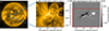 |
Fig. 1. Active region NOAA 12241. a) Full-disk image in 171 Å observed by SDO/AIA on December 18, 2014, at 21:24 UT. The blue rectangle indicates the active region under study. b) Zoom-in of the active region in 171 Å. c) LOS magnetogram taken by SDO/HMI. The red rectangle indicates the horizontal domain for the numerical simulation. |
2.2. Modelling the dynamics of NOAA AR 12241
To model the magnetic field of the active region, we used an NFFF extrapolation as initial condition. Briefly, this method is based on the principle of minimum energy dissipation rate, in which the magnetic field has to satisfy the double-curl Beltrami equation (see Bhattacharyya et al. 2007). Then, the magnetic field B can be written as B = B1 + B2 + B3, where  correspond to two linear force-free fields, and B3 with α3 = 0 corresponds to a potential field (Hu & Dasgupta 2008). The parameters α1, 2 were normalised by the horizontal grid size and chosen to minimise the value of the difference between the computed and measured transverse magnetic field vectors at the bottom boundary. For this active region, the values were α1 = 0.0105 and α2 = −0.0105. The units of α are pixel inverse, with a pixel size of 1 arcsec. For more details about the model, we refer to Hu et al. (2010) and references therein. The code for calculating an NFFF extrapolation for active or quiet regions is available online1. The linear combination of two linear force-free fields and one potential field causes the total field to be non-force-free (hence the name non-force-free field extrapolation). As we mentioned in Sect. 1, force-free extrapolation generally requires an external driver (e.g. photospheric flows or flux emergence) to trigger the eruption. In an NFFF extrapolation, the initial state is imbalanced, and this inherent force can drive an eruption (see Prasad et al. 2017, 2023). Previous experiments considering the same active region using earlier magnetograms, not shown in this paper for the sake of conciseness, indicated that such an initial imbalance state can also lead to a quiet relaxation of the system, without necessarily leading to an eruptive event.
In the case we present here, the NFFF initial condition induced the self-consistent development of a flux rope that subsequently rose and left the computational domain. This result was obtained by inserting the NFFF into a plane-parallel stratified atmosphere structured like the atmosphere of the Sun. It included a dense and cold lower layer similar to a chromosphere, a narrow transition region, and an extended and hot corona (for more details of the initial conditions, see Fig. A.1 and Fig. A.2 from Appendix A.3). The compressible MHD equations were then solved with the code PLUTO2 (Mignone et al. 2007) to study the evolution following this initial imbalance, including thermal conduction and radiative cooling. We defer a detailed description of the MHD modelling to Appendix A. More precisely, we describe the MHD equations we used in Appendix A.1, the numerical grid in Appendix A.2, the initial conditions in Appendix A.3, and the boundary conditions in Appendix A.4. We next describe the two stages of the dynamical evolution we obtained with our model.
2.2.1. Flux rope formation and mass loading
A summary of the evolution of the simulation is shown in Fig. 2. The top panels display the initial stage, and the bottom panels present the evolution of the rising structure. Initially, the plane-parallel atmosphere was in hydrostatic equilibrium, but the non-force-free magnetic field was imbalanced. Panel a shows at t = 0 s the magnetic field lines of an arcade (magenta lines) that are going to evolve into the eruptive flux rope and the non-zero Lorentz force (green to yellow iso-surfaces). Strong Lorentz force concentrations are found especially in the lower atmosphere (highlighted by the yellow patches), near the arcade footpoints. Thus, the out-of-equilibrium magnetic field destabilises the atmosphere, inducing motions and subsequent compression and heating of the plasma in the upper part of the transition region. This is shown in a small region highlighted by the grey square in panel b. The horizontal component of the Lorentz force (blue and red arrows) rapidly (t = 0.23 s) induces a flow that compresses the upper part of the transition region (around z = 2.5 Mm), close to the highlighted magnetic arcade. This compression causes a local increase in the temperature by a factor of 8 (yellow volumes at 4 × 10⁶ K in panel b). Thermal conduction then takes over, heating the top of the transition region from above, and eventually leading to evaporation. This evaporation fills up the magenta arcade with denser material, setting up the mass loading.
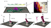 |
Fig. 2. Initialisation and evolution of the eruption at a glance. In all the panels, a magnetogram, with white to black levels, is present in the background to make the link with observations in Fig. 1. The colour map is saturated between −400 and 400 G for visualisation purposes. a) Initial magnetic configuration and Lorentz force at t = 0 s. The pink lines represent the magnetic arcade that was later on transformed into the erupting flux rope. The green to yellow colour map indicates a volumetric representation of the magnitude of the Lorentz force; yellow (green) is more (less) intense. b) Zoom-in at t = 0.23 s of the region defined by the grey rectangle in panel a. The horizontal components of the Lorentz force are shown with arrows in blue (negative) and red (positive), drawn at a height z = 2.2 Mm. Temperature iso-surfaces of 2 × 10⁶ K (red) to 4 × 10⁶ (yellow) are also displayed. c) Rising phase for t = 6.87 min, t = 9.92 min, and 12.59 min. The coloured lines represent the magnetic field lines corresponding to the flux rope. The colour of the field lines represents the vertical speed vz in pink. The two lines in the xy-plane indicate the cuts where the tracking (T line in light turquoise) of the flux rope and the compression (C line in dark turquoise) analysis were performed. |
After evaporation is initiated, reconnection between opposite legs of the arcade starts to take place (see Fig. C.1 from Appendix C for a quantitative description). This reconnection increases the twist of the arcade, leading to the formation of the flux rope.
2.2.2. Rise and escape of the flux rope
Later on in the simulation (see Fig. 2c), the flux rope expands and rises. As the flux rope rises, it carries up dense and hot material. This is shown in Fig. 3, where panel a exhibits the density and panel b the temperature in a yz-plane at x = 5 Mm for t = 12.59 min. This plane corresponds to the T line (light turquoise) from Fig. 2c and intersects the flux rope transversely near its the apex. The plasma is denser and hotter (in yellow) than in the surrounding corona, and it is delimited by ellipse-shaped field lines of the magnetic field projected onto the plane (white streamlines representing the magnetic field lines on that plane).
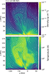 |
Fig. 3. Thermodynamical variables in the rising phase. a) Density and b) temperature at x = 5 Mm (corresponding to line T in Fig. 2c) for t = 12.59 min. Yellow denotes higher density and temperature, and blue shows lower values. The solid white lines represent the streamlines of the projected magnetic field vector on the plane. A movie showing the temperature in this cutting plane together with 3D visualisation of the flux rope field lines is available in the online version. |
Around t = 6 min, the interplay between the vertical gas pressure gradient and the Lorentz force gives a positive net contribution, and as a consequence, the fast rising motion is more evident (see Fig. 4) This figure shows in blue dots the z-coordinate of the apex of the flux rope identified in the same cutting plane as in Fig. 3, together with a quadratic fit (solid orange line). The apex is tracked until it leaves the domain at t = 16 min with a speed of about 350 km s−1. The identification and the tracking of the flux rope are explained in detail in Sect. 4.1. The legends with the arrows display the vertical speed of the flux rope apex vz, ap at x = 5 Mm obtained from the derivative of the fitting curve at a few selected times. As a consequence of the quadratic height profile, we obtained a vertical constant acceleration of 424 m s−2, which is 1.5 higher than the gravity at the solar surface.
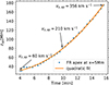 |
Fig. 4. Kinematic properties of the flux rope apex. We show the vertical coordinate of the flux rope apex at x = 5 Mm (blue dots) and quadratic fit (solid orange line). The values of the vertical velocity are added at different times. Before t = 4 min, the flux rope is not sufficiently well formed to infer the apex height. |
2.2.3. Energetics
To better understand the dynamics observed in our simulation, we complemented the previous simplified analysis with the overall evolution of the energy content in our simulation box, which is shown in Fig. 5. The total energy (solid black line) remains roughly constant, meaning that the losses (or gains) through the boundaries are small compared to the total energy content in the simulation box. The total magnetic energy (solid blue line) is similar to the total energy, showing that most of the energy in the domain is due to the magnetic field. From the calculation of the potential field (following the method proposed by Alissandrakis 1981), we estimated the magnetic energy associated with it and the free magnetic energy (dashed blue line) as Emag, free = Emag, tot − Emag, pot. We note that Emag, pot is almost constant in time because the magnetogram does not evolve (it slowly diminishes over the course of the simulation due to diffusion at the bottom boundary). This decrease in the potential energy is very small and does not affect the evolution of the free magnetic energy. The free magnetic energy originated from the NFFF extrapolation initially had a value of ∼3 × 1032 erg and then diminished because of ohmic dissipation, reaching a minimum at t = 2.6 min (second dotted vertical line). This decrease corresponds to an increase in the internal energy (solid green line) and a sudden increase in kinetic energy (solid orange line) to t = 0.40 min (first dotted line). After t = 2.6 min, the free magnetic energy slowly increased up to t = 16.3 min (third vertical dotted line) as the plasma motions caused the increase in the magnetic strength of the arcades. This rise is compensated for with a decrease in kinetic energy, mostly due to the work of the magnetic tension, and, to a lesser extent, because of other high-speed mass leaving the domain on the sides or through the top boundary. However, after t = 10 min, there is a slight increase in kinetic energy to t = 16.3 min. This is likely caused by the accelerated flux rope that ascends until it leaves the domain at t = 16.3 min. After this time, the free magnetic and kinetic energies both drop smoothly because of magnetic relaxation and the departure of the magnetic flux rope from the simulation box. In the next sections, we explain the different phenomena involved in the formation of the flux rope (Sect. 3) and its rising phase (Sect. 4) in more detail.
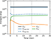 |
Fig. 5. Evolution of energies averaged in the entire computational domain. The total energy is shown as the solid black line, the total magnetic energy is shown as the solid blue line, the free magnetic energy is shown as the dashed blue line, and the kinetic and internal energies are shown as solid orange and green lines, respectively. The vertical dotted lines indicate different stages. |
3. Flux rope formation and plasma evaporation
In this section, we describe the initial stage of the simulation, which is crucial in the triggering of the eruption. Since the dynamics is very fast at the beginning, we ran the simulation using high temporal cadence outputs, every 0.11 s, to study the evolution of all the variables and the physical processes involved.
3.1. Role of the initial Lorentz force
Because the extrapolation is non-force-free, the initial Lorentz force is out of equilibrium (J × B ≠ 0). In particular, its horizontal components along the x- and y-axis point in opposite converging directions near the onset of the eruption, around x = −15 Mm, y = −7 Mm, in the vicinity of the polarity inversion line. This imbalance in the Lorentz force triggers a converging flow that causes compression of the plasma in the upper part of the transition region in a fraction of seconds. This is shown in Fig. 6, where panel a displays one of the horizontal components of the Lorentz force (J × B)y in a plane corresponding to x = −15.14 Mm (turquoise line C in Fig. 2 panel c) in a small region of the computational domain. The direction of the force is shown by the negative (blue) and positive (red) values.
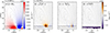 |
Fig. 6. Lorentz force and energy source terms for the plane x = −15 Mm (see its photospheric trace C in Fig. 2). a) Lorentz force on the y-axis at t = 0 s (positive values are shown in red, and negative values are shown in blue), b) compression, c) advection, and d) radiative cooling at t = 0.23 s (positive values are indicated in dark orange, and negative values are shown in purple). The upper limit of the transition region is denoted with the solid black line. |
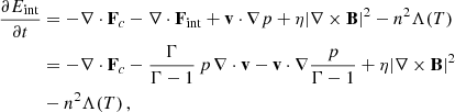
Panel b of Fig. 6 shows the compression term at t = 0.23 s for the same plane defined by line C. This term was obtained from the combination of the flux of the internal energy and the work of the pressure gradient from the internal energy equation and is proportional to ∇ ⋅ v (see Eq. (A.9)). The purple colour corresponds to negative contribution and orange to positive values. Panels c and d exhibit the contribution of the internal energy advection term and the radiative cooling, respectively, for the same time and plane. Γ = 5/3 is the ratio of specific heats, and p/(Γ − 1) corresponds to the internal energy, while n is the density number and Λ is the radiative loss function defined in Sect. A.1 by Eq. (A.8). The grey lines in the background of all panels correspond to the integral lines of the field components contained in the plane x = −15.14 Mm. The solid horizontal black lines denote the upper limit of the transition region, that is, the beginning of the corona. To calculate it, we searched for the minimum of the second derivative of the temperature with respect to height for each value of y.
Panel b shows that the localised compression between z = 1.5 Mm and z = 4.5 Mm and around y = −7.5 Mm is in the same location in which (J × B)y converges. Panel c illustrates that the advection term contributes with both positive and negative effects, although with smaller amounts. Moreover, the advection term is mostly important on the right side of the flux rope. Finally, panel d indicates that radiative cooling mostly removes energy from the system below the transition region as expected.
As a consequence of the initial compression due to converging flows triggered by the initial distribution of the Lorentz force, the density and temperature locally increase with time. To illustrate this effect in more detail, we present in Fig. 7b the temperature profile as a function of the distance for a single field line that is part of the flux rope, at different times. The times are represented by different line styles. The chosen field line has undergone marginal slippage during the times we analysed at this early stage. To verify this, we computed the squashing factor (not shown here for brevity) in the bottom plane where the field lines are rooted. For the positions of the left footpoint, we obtained values of |log(Q)| ∼ 1, and for the right footpoint, we obtained |log(Q)| ∼ 2. These values are lower than |log(Qmax)| ∼ 6 for this plane, suggesting that there is no strong field line slippage along the field line in this time interval for these locations. The displacements of the field line footpoints are negligible. Next, to highlight the process in the transition region, the field line was divided into two parts, one part from the left footpoint to the apex (top panel), and the other part from the right footpoint to the apex (bottom panel). The increase in temperature over time at either side of the apex of the field line is very noticeable, from 5 × 10⁵ K to 5 × 10⁷ K, especially in the lower corona, where the compression occurs. The x and y coordinates of this field line at the different times are shown in panel a, together with Bz at z = 0.05 Mm in the background. The method we used to identify and track the flux rope is explained in Sect. 4.1.
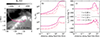 |
Fig. 7. Evolution of thermodynamical variables along a magnetic field line. a) We show the plane-of-sky coordinates of a magnetic field line, represented with dotted (t = 0 s), dashed (t = 0.23 s), dash-dotted (t = 1.14 s), and solid lines (t = 13.74 s), from light to dark pink. In the background, Bz at z = 0.05 Mm and t = 0 s is shown in greyscale, with negative values in black and positive values in white. b) Temperature. c) Vertical velocity along the field line from the left footpoint to the apex (top panels) and from the right footpoint to the apex (bottom panels). The variables are plotted for the same instants in time as in panel a. |
3.2. Thermal conduction and evaporation
Immediately after the compression begins, the temperature increases, as previously described, and a downflow occurs at either side of the region that is heated. Because of the temperature rise at the apex, the thermal conduction flux grows in time along the magnetic field lines, heating the plasma at the bottom of the transition region. As a consequence, some hot material starts to move upwards from the transition region, that is, it evaporates. In Fig. 7c we present the vertical velocity vz along the field line for the same time steps as described in panels a and b. The field line is also divided into two parts to show the evaporation above the transition region in more detail. At t = 0.23 s (dashed line), a flux moves downwards (top panel) near the location where the plasma is heated (see the corresponding peak in temperature in panel b, around 2 and 3 Mm.
After the plasma has been heated, around t = 1.14 s (dash-dotted line), a flux ascends from the transition region to the corona, and from t = 13.74 s onwards, this upflow remains and increases on one side of the field line (left footpoint). This upflow loads the whole flux rope with mass during these initial stages of the simulation.
4. Flux rope rise and deflection
As evaporation and reconnection persist in the lower part of the flux rope, the magnetic field lines belonging to it are loaded with mass while they continue to expand and twist. At about t = 4 min, the flux rope is well defined and starts to rise slowly, driven by a net upward force that is a combination of the Lorentz force and the gas pressure gradient. As the structure moves upwards, it is deflected south-east, in the same direction as in observations, towards a region of low magnetic pressure. In this section, we describe the dynamical analysis of the forces acting on the flux rope in the rising phase.
4.1. Flux rope identification
To identify and track the flux rope in time, we used GUITAR (Graphical User Interface for Tracking and Identifying flux Ropes3, Wagner et al. 2024a,c). The method uses combinations of mathematical morphology algorithms, such as erosion and dilatation, to extract the magnetic flux rope throughout a time series. More details about the method are given in Appendix B. A flux rope is a group of helical field lines that collectively winds around a common axis (Liu 2020). The winding number 𝒯g (see Eq. 12 in Berger & Prior 2006) quantifies the number of turns made around the flux rope axis for each field line. For 3D magnetic configurations, one of the difficulties for calculating 𝒯g is to find the flux rope axis. An easier quantity to compute is the twist number, which is defined by
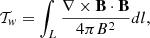
where ∇ × B is the current density, dl is the elementary length along the field line, and L is the total length of the studied field line. 𝒯w supplies the number of turns that two infinitesimally adjacent field lines make around each other (Berger & Prior 2006). 𝒯w is an approximation of 𝒯g. More precisely, 𝒯w approaches 𝒯g in the vicinity of the axis of a nearly cylindrically symmetric flux tube (Liu et al. 2016). To determine the location of the flux rope axis, assumptions are necessary and often involve the computation of 𝒯w, where the axis is assumed to be located at a local extrema of 𝒯w (Liu et al. 2016; Price et al. 2024). In contrast, 𝒯w can be computed straightforwardly for any field line, and for the case of thin flux ropes, the errors are rather small (for more details see Liu et al. 2016; Liu 2020).
We applied GUITAR to 𝒯w calculated along the field lines that go through a 2D plane located at x = 5 Mm (cut T in Fig. 2), shown in Fig. 8. This figure displays the evolution of 𝒯w for a) t = 7.63 min, b) t = 8.78 min, and c) t = 9.92 min in green (negative) to pink (positive) colour map. The grey circles correspond to the location of the flux rope extracted with GUITAR. The flux rope is associated with a highly coherent twisted structure that remains connected to the photosphere during the entire rising phase until it leaves the domain. As the flux rope moves upwards, a current layer of opposite twist number (𝒯w < 0) develops at its boundary.
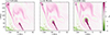 |
Fig. 8. Twist 𝒯w at x = 5 Mm (cut T in Fig. 2) for a) t = 7.63 min, b) t = 8.78 min, and c) t = 9.92 min. Pink indicates positive values of twist related to a current density parallel to the magnetic field for the corresponding field line, and green denotes the anti-parallel orientation. The grey circles represent the points belonging to the flux rope extracted with GUITAR. |
The chosen plane transversely cuts the flux rope through the apex. Since the magnetic structure is deflected while it ascends, the apex location is shifted. Therefore, the transverse plane containing the apex changes as well. Nevertheless, the x-coordinate of the apex of the flux rope remains near the chosen plane during most of the rising phase. We extracted the points that correspond to the flux rope in this plane, and from these points, we traced the magnetic field lines down to the photosphere. These seeds were used to trace the early evolution of the flux rope, as shown for instance in Fig. 7, and for the following analysis of forces and deflection, we used the seeds extracted with GUITAR at x = 5 Mm.
4.2. Force balance and rising phase
In this section, we analyse the forces involved in the upwards motion of the flux rope. In the top panels of Fig. 9, we consider the net vertical force, which includes the Lorentz force, the gas pressure gradient, advection, and gravity (all the terms included in the momentum Eq. (A.2)) at z = 24 Mm, which corresponds to the height at which the forces reach their maximum value. The colour scale is shown on the right side from blue (negative) to red (positive) colour (white corresponds to zero). The panels are taken at a) t = 4.5 min, b) t = 4.96 min, c) t = 6.11 min, d) t = 7.63 min, and e) t = 8.78 min. The grey contours depict values of the vertical component of the magnetic field Bz at the photosphere (dashed line for −400 G and solid for 400 G). The green contours represent different values of vertical speed. The magenta lines show the field lines belonging to the flux rope, darker segments of these lines are above z = 24 Mm.
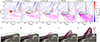 |
Fig. 9. Top panels: Evolution of the net vertical force (positive values are plotted in red, and negative values are shown in blue) at z = 24 Mm for a) t = 4.5 min, b) t = 4.96 min, c) t = 6.11 min, d) t = 7.63 min, and e) t = 8.78 min. The magenta lines correspond to field lines computed within the flux rope. The grey contours indicate positive (solid) and negative (dashed) values of Bz at z = 0.05 Mm, and the green contours exhibit different values of vz between 218 (dark green) and 436 km s−1 (light green). Bottom panels: Flux rope magnetic field lines in 3D coloured by vz for the same times as in the top panels. The semi-transparent grey plane corresponds to z = 24 Mm and contains the same vz contours as the top panels. |
The rising motion is clearly visible in the 3D field lines of Fig. 9, panels h to j, where the height of the flux rope and the vertical speed increase notably, in contrast to panels f to h, where the height of the flux rope remains practically constant and the vertical speed increases gradually.
Panels a to c of Fig. 9 show a portion of plasma moving upwards and south-west (y decreases and x increases), indicated by the displacement and enhancement of the net vertical force. The positive value of this net vertical force mostly comes from the advection term (see Fig. D.1, fourth row). This net force was computed with an Eulerian viewpoint, and then, the local acceleration of the plasma at a fixed spatial position is mainly due to the transfer (advection) of the plasma from lower layers. As expected, the location of the strong vertical velocity (green contours) follows the same evolution. The net force then decreases, as shown from the evolution in panels b to c.
Following this upward expansion, the fast rising motion of the flux rope is triggered, indicated in panels c to e by the contours of higher vz and once again, the enhancement of the net vertical force towards the south-east. At this stage, the increase in the net force is due to the positive total contribution of the gas pressure gradient and the Lorentz force (see Fig. D.1, third row). The rising motion is accompanied by a deviation of the x apex coordinate of the flux rope, which we call deflection. Before t = 5 min, the apex moves south-west, and then it moves south-east. The deflection is described in detail in the next section.
4.3. Deflection
During the rising motion, the flux rope is chanelled into regions of low magnetic magnetic pressure, causing a deflection of the eruption. This can be observed in Fig. 10, where we show the magnetic pressure for z = 60 Mm, where blue corresponds to lower values and yellow to high values. The different panels represent different times, being a) t = 7.63 min, b) 8.78 min, and c) t = 9.92 min. We also display magnetic field lines representing different parts of the erupting flux rope in magenta, where the brighter parts in it indicate that they are above the horizontal cutting plane (z = 60 Mm). We also include plasma β = p/pm contours, with p corresponding to the gas pressure and pm = B2/8π the magnetic pressure. The regions in which β = 10 (yellow contours) correspond to the flux rope. As the flux rope ascends, magnetic reconnection occurs at the leading edge and right flank of the structure, which strongly decreases the magnetic pressure and increases the plasma pressure, hence, increasing the values of β. This is a consequence of the evolution of the initial NFFF, since initially, there are no regions with β = 10 at this height (see Fig. A.1, panel b), and it is a highly dynamic feature since the speed of the flux rope is super-Alfvénic at this stage (as also visible in the strong contribution of advection to the evolution of the flux rope in Appendix D).
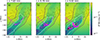 |
Fig. 10. Evolution of the magnetic pressure at z = 60 Mm for (a) t = 7.63 min, (b) 8.78 min, and (c) t = 9.92 min. The background colour shows the variation in B2/8π in a blue-to-yellow colour map, with blue being the lowest and yellow the highest value. The different field lines displayed in magenta correspond to the apex and to the left and right flanks of the flux rope. The contours show different values of β of 0.1 (indigo), 1 (white), and 10 (yellow). |
Figure 10 shows that as the simulation evolves, the field lines representing the flux rope are deflected towards a region with low magnetic pressure in the x − y plane, denoted by dark blue colours, and crossing the cutting plane where β > 1. We also verified the behaviour of the gas pressure for this height (not shown here) and confirm that the gas pressure increases, but in a manner not as localised as the decrease in the magnetic pressure. This suggests that the deflection is affected by the decrease in the magnetic pressure, which agrees with previous observational studies (Gui et al. 2011; Liewer et al. 2015; Sieyra et al. 2020).
5. Discussion and conclusions
We performed a resistive full-MHD simulation of the flaring active region NOAA 12241, considering an initial situation composed of a magnetic field obtained from an NFFF extrapolation together with a plane-parallel atmosphere ranging from the photosphere to the corona. The extrapolation was based on a vector magnetogram taken by SDO/HMI a few minutes before the onset of the flare. In this simulation, a flux rope formed due to the converging Lorentz force acting on the initial sheared arcade, carrying dense material from the photosphere. In the initial stage, this converging force produced compression and locally heated the plasma above the transition region. This also resulted in the evaporation of plasma that filled the flux rope with dense material. Plasma evaporation driven by compression and thermal conduction was demonstrated by Donné et al. (2026) in 2.5D simulations.
As the flux rope rises, as a result of a net upwards force, it is deflected towards regions of low magnetic pressure. This agrees with the SDO/AIA observations of this event and with previous observational studies of other deflected eruptive events (Gui et al. 2011; Liewer et al. 2015; Sieyra et al. 2020). Finally, the flux rope left the domain after 16 minutes since initialisation of the simulation, with a vertical speed of approximately 350 km s−1. To identify the flux rope and characterise its dynamics, we used GUITAR (Wagner et al. 2024a,c), which is an algorithm designed for identifying and tracking magnetic structures using the twist as a proxy.
Compared with other force-free models that minimise the total magnetic energy and assume β ≈ 0, the NFFF extrapolation follows an alternative approach by minimising the total energy dissipation rate, which considers more generalised momentum balance equations supporting a finite plasma pressure (see discussion in Hu et al. 2008, 2010). As a result, the magnetic field obtained from this type of extrapolation presents a non-vanishing Lorentz force in the low atmosphere. On one hand, this allowed us to simulate the dynamics of the plasma near the onset of the eruption, having converging and shearing forces from the very beginning. This reduced the computational time of the energy build-up and the need of triggering the eruption through the external photospheric driving. On the other hand, since the initial components of the Lorentz force originate from the extrapolation itself, we had no control of the intensity and direction of the shearing and converging motions. Another limitation is that the parameters αi that define the NFFF magnetic field (B = B1 + B2 + B3, where ∇ × Bi = αiBi with i ∈ (1, 2, 3)) are constrained by the size of the horizontal grid (used to normalised αi) since αmax = 2π/N, where N is the number of grid points, and the assumption of periodic boundary conditions on the sides (because the calculation of the force free fields includes Fourier transforms). Nevertheless, Bhattacharyya et al. (2007) demonstrated that arcade structures can be modelled as relaxed states using the minimum dissipation rate principle, a hypothesis that we assumed for NFFF extrapolations. Moreover, several recent studies used an MHD simulation initiated with the NFFF that successfully explained various transient events in active regions, such as flares, coronal jets, and coronal dimmings (Prasad et al. 2018, 2020, 2023; Nayak et al. 2019).
In terms of kinematics, Fig. 4 shows that the vertical speed for the apex of the flux rope agrees with the fast phase speed of the observed flux rope shown in Fig. 7b from Joshi et al. (2017) (taking into account that the observed speed is a projected value on the plane of sky). The slow phase in our model lasted until ∼6 min. Since the model was initiated very close in time to the onset of the flare with an imbalanced magnetic field, the initial compression and twist build-up of the flux rope occurred faster than in observations (∼18 min). After the slow phase was completed, around 6 min, the erupting flux rope exhibited a ballistic propagation with a constant acceleration of 424 m s−2 (1.5 higher than solar gravity). We can consider that this is the start of the fast or accelerated phase. However, as also stated by Jiang (2024), it is difficult to precisely determine the beginning of the eruption phase. In non-ideal models from the literature, the acceleration of the eruptive flux rope is related to magnetic reconnection, which causes impulsive acceleration. Inoue et al. (2025) showed how a small flux emergence reconnected with the ambient field. By comparing simulations, one simulation obtained from an evolved data-driven model and the other simulation obtained from a data-constrained model including flux emergence, both initialised with NLFFF extrapolations and plasma β = 0, the authors obtained that in the initial stage, both simulations were dynamically similar. However, just after the triggering of the acceleration phase, the vertical velocities started to diverge, with the data-constrained simulation showing higher acceleration than the data-driven simulation.
Another point to consider is the atmospheric profile that was chosen here, and how it affects the dynamics, density, and temperature of the flux rope. To address this point, we performed another simulation with the same magnetic field, but with a smoother and higher transition region (still using a plane-parallel stratified initial condition). The simulation was not shown here for the sake of conciseness, but it showed qualitatively the same behaviour as the simulation presented in this work. Still, some differences are notable when considering this wider transition region. First, the dynamics are slightly altered, and the eruption is delayed for more than 6 minutes. Similar results were shown by Rice & Prior (2025) with 2.5 MHD simulations considering different temperature profiles. In this other simulation, the rising phase starts later than in the simulation presented in this work, because heavier material takes more time to be lifted up, and hence, the flux rope leaves the domain later with a lower speed of 250 km s−1. Second, concerning the thermodynamical structure of the flux rope, changing the profile of the transition region modifies the density and temperature of the flux rope. We found for the higher transition region that the flux rope is almost twice as dense and cold than the atmosphere profile analysed in this work, and this affects the emission. Therefore, when observational features are to be reproduced, it is of the upmost importance to consider a realistic atmosphere. In a forthcoming paper, we aim to quantitatively explore the synthetic emission obtained from the simulations, which was not included here because the focus of the paper was to present the model and describe the dynamics.
Finally, our compressible full-MHD simulation results are comparable with the outcomes from the incompressible and isothermal simulation of Prasad et al. (2023) (see the discussion in Introduction) in the fact that the eruption is triggered by the converging Lorentz force in the lower atmosphere exerted on a sheared arcade that later develops into a flux rope. However, the authors pointed out that in their simulations, the rising motion of the flux rope ceased towards the end, whereas in our case, the flux rope left the domain at a constant acceleration. We also note that gravity can slow the escaping flux rope down, but in this case, it acts too slowly to affect its speed. The two simulations started from the same initial extrapolation, which strikingly shows that our use of fully compressible MHD affects the predicted characteristics of the escaping flux rope.
As future prospects, we intend to include flux emergence in our simulation framework (as for example in Inoue et al. 2025; Moreno-Insertis et al. 2025). We are also working towards estimating non-thermal emissions from the inclusion of test-particles in the simulation.
Data availability
Movie associated with Fig. 3 is available at https://www.aanda.org
Acknowledgments
We sincerely thank the referee for the constructive feedback, which has improved the clarity and quality of this manuscript. This work has been supported by the French Agence Nationale de la Recherche (ANR) project STORMGENESIS #ANR-22-CE31-0013-01, the European Research Council through the Synergy Grant number 810218 (“The Whole Sun”, ERC-2018-SyG), the Centre National d’Etudes Spatiales (CNES) Solar Orbiter project, the Institut National des Sciences de l’Univers (INSU) via the Action Thématique Soleil-Terre (ATST), and Programme for Supercomputing, and by computing HPC and storage resources by GENCI thanks to the grants 2023-A0140410133, 2024-A0160410133 and 2025-A0180410133. AW acknowledges the Finnish Centre of Excellence in Research of Sustainable Space (Research Council of Finland grant numbers 352850). AW also acknowledges the Space Weather Awareness Training Network (SWATNet) which has received funding from the European Union’s Horizon 2020 research and innovation programme under the Marie Skłodowska-Curie Innovative Training Networks, Grant Agreement No 955620. RJ acknowledges research support from the Research Council of Norway, project number 325491, through its Centres of Excellence scheme, project number 262622.
References
- Afanasyev, A. N., Fan, Y., Kazachenko, M. D., & Cheung, M. C. M. 2023, ApJ, 952, 136 [Google Scholar]
- Agarwal, S., Bhattacharyya, R., & Wiegelmann, T. 2022, Sol. Phys., 297, 91 [Google Scholar]
- Alissandrakis, C. E. 1981, A&A, 100, 197 [NASA ADS] [Google Scholar]
- Amari, T., Luciani, J. F., Aly, J. J., Mikic, Z., & Linker, J. 2003, ApJ, 595, 1231 [Google Scholar]
- Amari, T., Canou, A., & Aly, J.-J. 2014, Nature, 514, 465 [NASA ADS] [CrossRef] [Google Scholar]
- Antiochos, S. K., DeVore, C. R., & Klimchuk, J. A. 1999, ApJ, 510, 485 [Google Scholar]
- Athay, R. G. 1986, ApJ, 308, 975 [Google Scholar]
- Aulanier, G., Démoulin, P., & Grappin, R. 2005, A&A, 430, 1067 [NASA ADS] [CrossRef] [EDP Sciences] [Google Scholar]
- Aulanier, G., Török, T., Démoulin, P., & DeLuca, E. E. 2010, ApJ, 708, 314 [Google Scholar]
- Benz, A. O. 2017, Liv. Rev. Sol. Phys., 14, 2 [Google Scholar]
- Berger, M. A., & Prior, C. 2006, J. Phys. Math. Gener., 39, 8321 [Google Scholar]
- Bhattacharyya, R., & Janaki, M. S. 2004, Phys. Plasmas, 11, 5615 [NASA ADS] [CrossRef] [Google Scholar]
- Bhattacharyya, R., Janaki, M. S., Dasgupta, B., & Zank, G. P. 2007, Sol. Phys., 240, 63 [NASA ADS] [CrossRef] [Google Scholar]
- Carmichael, H. 1964, in NASA Special Publication, ed. W. N. Hess, 50, 451 [NASA ADS] [Google Scholar]
- Chen, F., Cheung, M. C. M., Rempel, M., & Chintzoglou, G. 2023, ApJ, 949, 118 [NASA ADS] [CrossRef] [Google Scholar]
- Cheung, M. C. M., & DeRosa, M. L. 2012, ApJ, 757, 147 [NASA ADS] [CrossRef] [Google Scholar]
- Daei, F., Pomoell, J., Price, D. J., et al. 2023, A&A, 676, A141 [NASA ADS] [CrossRef] [EDP Sciences] [Google Scholar]
- Donné, D., Zhou, Y., Cremades, H., & Keppens, R. 2026, A&A, 707, A375 [NASA ADS] [CrossRef] [EDP Sciences] [Google Scholar]
- Fan, Y. 2011, ApJ, 740, 68 [Google Scholar]
- Fan, Y. 2022, ApJ, 941, 61 [Google Scholar]
- Fletcher, L., Dennis, B. R., Hudson, H. S., et al. 2011, Space Sci. Rev., 159, 19 [Google Scholar]
- Gardiner, T. A., & Stone, J. M. 2005, J. Comput. Phys., 205, 509 [NASA ADS] [CrossRef] [Google Scholar]
- Gary, G. A. 2001, Sol. Phys., 203, 71 [Google Scholar]
- Gibb, G. P. S., Mackay, D. H., Green, L. M., & Meyer, K. A. 2014, ApJ, 782, 71 [NASA ADS] [CrossRef] [Google Scholar]
- Gui, B., Shen, C., Wang, Y., et al. 2011, Sol. Phys., 271, 111 [NASA ADS] [CrossRef] [Google Scholar]
- Guo, J. H., Ni, Y. W., Zhong, Z., et al. 2023, ApJS, 266, 3 [NASA ADS] [CrossRef] [Google Scholar]
- Guo, J. H., Ni, Y. W., Guo, Y., et al. 2024, ApJ, 961, 140 [NASA ADS] [CrossRef] [Google Scholar]
- Hirayama, T. 1974, Sol. Phys., 34, 323 [Google Scholar]
- Hood, A. W., & Priest, E. R. 1979, Sol. Phys., 64, 303 [NASA ADS] [CrossRef] [Google Scholar]
- Hu, Q., & Dasgupta, B. 2008, Sol. Phys., 247, 87 [Google Scholar]
- Hu, Q., Dasgupta, B., Choudhary, D. P., & Büchner, J. 2008, ApJ, 679, 848 [Google Scholar]
- Hu, Q., Dasgupta, B., Derosa, M. L., Büchner, J., & Gary, G. A. 2010, J. Atmosph. Sol.-Terr. Phys., 72, 219 [Google Scholar]
- Inoue, S. 2016, Prog. Earth Planet. Sci., 3, 19 [CrossRef] [Google Scholar]
- Inoue, S., Kusano, K., Büchner, J., & Skála, J. 2018, Nat. Commun., 9, 174 [NASA ADS] [CrossRef] [Google Scholar]
- Inoue, S., Miyoshi, T., Hayashi, K., et al. 2025, ApJ, 988, L36 [Google Scholar]
- Janvier, M., Aulanier, G., Bommier, V., et al. 2014, ApJ, 788, 60 [Google Scholar]
- Ji, H., Wang, H., Schmahl, E. J., Moon, Y.-J., & Jiang, Y. 2003, ApJ, 595, L135 [NASA ADS] [CrossRef] [Google Scholar]
- Jiang, C. 2024, Sci. China Earth Sci., 67, 3765 [Google Scholar]
- Jiang, C., & Feng, X. 2014, Sol. Phys., 289, 63 [NASA ADS] [CrossRef] [Google Scholar]
- Jiang, C., Feng, X., Wu, S. T., & Hu, Q. 2013, ApJ, 771, L30 [Google Scholar]
- Jiang, C., Wu, S. T., Feng, X., & Hu, Q. 2016, Nat. Commun., 7, 11522 [NASA ADS] [CrossRef] [Google Scholar]
- Jiang, C., Feng, X., Guo, Y., & Hu, Q. 2022, The Innovation, 3, 100236 [NASA ADS] [CrossRef] [Google Scholar]
- Joshi, N. C., Sterling, A. C., Moore, R. L., Magara, T., & Moon, Y.-J. 2017, ApJ, 845, 26 [NASA ADS] [CrossRef] [Google Scholar]
- Joshi, R., Aulanier, G., Radcliffe, A., et al. 2024a, A&A, 687, A172 [NASA ADS] [CrossRef] [EDP Sciences] [Google Scholar]
- Joshi, R., Rouppe van der Voort, L., Schmieder, B., et al. 2024b, A&A, 691, A198 [NASA ADS] [CrossRef] [EDP Sciences] [Google Scholar]
- Kilpua, E. K. J., Pomoell, J., Price, D., Sarkar, R., & Asvestari, E. 2021, Front. Astron. Space Sci., 8, 35 [NASA ADS] [CrossRef] [Google Scholar]
- Kliem, B., & Török, T. 2006, Phys. Rev. Lett., 96, 255002 [Google Scholar]
- Kopp, R. A., & Pneuman, G. W. 1976, Sol. Phys., 50, 85 [Google Scholar]
- Kumar, S., Prasad, A., Sarkar, R., & Bhattacharyya, R. 2022, Front. Astron. Space Sci., 9, 1039061 [NASA ADS] [CrossRef] [Google Scholar]
- Kumar, S., Kumar, P., Sadashiv, S., et al. 2025, Sol. Phys., 300, 22 [Google Scholar]
- Leake, J. E., Linton, M. G., & Antiochos, S. K. 2010, ApJ, 722, 550 [Google Scholar]
- Leake, J. E., Linton, M. G., & Antiochos, S. K. 2014, ApJ, 787, 46 [NASA ADS] [CrossRef] [Google Scholar]
- Leake, J. E., Linton, M. G., & Antiochos, S. K. 2022, ApJ, 934, 10 [CrossRef] [Google Scholar]
- Lemen, J. R., Title, A. M., Akin, D. J., et al. 2012, Sol. Phys., 275, 17 [Google Scholar]
- Liewer, P., Panasenco, O., Vourlidas, A., & Colaninno, R. 2015, Sol. Phys., 290, 3343 [Google Scholar]
- Linker, J. A., Mikić, Z., Lionello, R., et al. 2003, Phys. Plasmas, 10, 1971 [Google Scholar]
- Liu, R. 2020, RAA, 20, 165 [Google Scholar]
- Liu, R., Kliem, B., Titov, V. S., et al. 2016, ApJ, 818, 148 [Google Scholar]
- Londrillo, P., & del Zanna, L. 2004, J. Comput. Phys., 195, 17 [NASA ADS] [CrossRef] [Google Scholar]
- Lynch, B. J., Antiochos, S. K., DeVore, C. R., Luhmann, J. G., & Zurbuchen, T. H. 2008, ApJ, 683, 1192 [NASA ADS] [CrossRef] [Google Scholar]
- MacTaggart, D., & Haynes, A. L. 2014, MNRAS, 438, 1500 [Google Scholar]
- Mignone, A., Bodo, G., Massaglia, S., et al. 2007, ApJS, 170, 228 [Google Scholar]
- Moore, R. L., Sterling, A. C., Hudson, H. S., & Lemen, J. R. 2001, ApJ, 552, 833 [Google Scholar]
- Moreno-Insertis, F., Hansteen, V. H., & Nóbrega-Siverio, D. 2025, ApJ, 995, 137 [Google Scholar]
- Muhamad, J., Kusano, K., Inoue, S., & Shiota, D. 2017, ApJ, 842, 86 [Google Scholar]
- Nayak, S. S., Bhattacharyya, R., Prasad, A., et al. 2019, ApJ, 875, 10 [Google Scholar]
- Pariat, E., Antiochos, S. K., & DeVore, C. R. 2010, ApJ, 714, 1762 [NASA ADS] [CrossRef] [Google Scholar]
- Pesnell, W. D., Thompson, B. J., & Chamberlin, P. C. 2012, Sol. Phys., 275, 3 [Google Scholar]
- Pomoell, J., Lumme, E., & Kilpua, E. 2019, Sol. Phys., 294, 41 [NASA ADS] [CrossRef] [Google Scholar]
- Prasad, A., Bhattacharyya, R., & Kumar, S. 2017, ApJ, 840, 37 [NASA ADS] [CrossRef] [Google Scholar]
- Prasad, A., Bhattacharyya, R., Hu, Q., Kumar, S., & Nayak, S. S. 2018, ApJ, 860, 96 [NASA ADS] [CrossRef] [Google Scholar]
- Prasad, A., Dissauer, K., Hu, Q., et al. 2020, ApJ, 903, 129 [Google Scholar]
- Prasad, A., Kumar, S., Sterling, A. C., et al. 2023, A&A, 677, A43 [NASA ADS] [CrossRef] [EDP Sciences] [Google Scholar]
- Price, D. J., Pomoell, J., Lumme, E., & Kilpua, E. K. J. 2019, A&A, 628, A114 [NASA ADS] [CrossRef] [EDP Sciences] [Google Scholar]
- Price, D. J., Pomoell, J., & Kilpua, E. K. J. 2020, A&A, 644, A28 [NASA ADS] [CrossRef] [EDP Sciences] [Google Scholar]
- Price, D. J., Pomoell, J., & Kilpua, E. K. J. 2024, A&A, 686, A197 [NASA ADS] [CrossRef] [EDP Sciences] [Google Scholar]
- Réville, V., Velli, M., Panasenco, O., et al. 2020, ApJS, 246, 24 [Google Scholar]
- Réville, V., Jasinski, J. M., Velli, M., et al. 2024, ApJ, 976, 65 [CrossRef] [Google Scholar]
- Rice, O., & Prior, C. 2025, ApJ, 981, 86 [Google Scholar]
- Schou, J., Scherrer, P. H., Bush, R. I., et al. 2012, Sol. Phys., 275, 229 [Google Scholar]
- Schuck, P. W., Linton, M. G., Knizhnik, K. J., & Leake, J. E. 2022, ApJ, 936, 94 [Google Scholar]
- Scott, R. B., Pontin, D. I., & Hornig, G. 2017, ApJ, 848, 117 [NASA ADS] [CrossRef] [Google Scholar]
- Shibata, K., & Magara, T. 2011, Liv. Rev. Sol. Phys., 8, 6 [Google Scholar]
- Sieyra, M. V., Cécere, M., Cremades, H., et al. 2020, Sol. Phys., 295, 126 [NASA ADS] [CrossRef] [Google Scholar]
- Sturrock, P. A., & Coppi, B. 1965, AJ, 70, 331 [Google Scholar]
- Tassev, S., & Savcheva, A. 2017, ApJ, 840, 89 [NASA ADS] [CrossRef] [Google Scholar]
- Titov, V. S., & Démoulin, P. 1999, A&A, 351, 707 [NASA ADS] [Google Scholar]
- Titov, V. S., Downs, C., Mikić, Z., et al. 2018, ApJ, 852, L21 [NASA ADS] [CrossRef] [Google Scholar]
- Török, T., Kliem, B., & Titov, V. S. 2004, A&A, 413, L27 [NASA ADS] [CrossRef] [EDP Sciences] [Google Scholar]
- Török, T., Downs, C., Linker, J. A., et al. 2018, ApJ, 856, 75 [Google Scholar]
- Valori, G., Démoulin, P., Pariat, E., & Masson, S. 2013, A&A, 553, A38 [NASA ADS] [CrossRef] [EDP Sciences] [Google Scholar]
- Wagner, A., Bourgeois, S., Kilpua, E. K. J., et al. 2024a, A&A, 683, A39 [NASA ADS] [CrossRef] [EDP Sciences] [Google Scholar]
- Wagner, A., Price, D. J., Bourgeois, S., et al. 2024b, A&A, 692, A74 [NASA ADS] [CrossRef] [EDP Sciences] [Google Scholar]
- Wagner, A., Price, D. J., Bourgeois, S., et al. 2024c, Front. Astron. Space Sci., 11, 1383072 [NASA ADS] [CrossRef] [Google Scholar]
- Wang, X., Jiang, C., & Feng, X. 2023, ApJ, 942, L41 [Google Scholar]
- Wheatland, M. S., & Gilchrist, S. A. 2013, J. Phys. Conf. Ser., 440, 012037 [Google Scholar]
- Wiegelmann, T., & Sakurai, T. 2021, Liv. Rev. Sol. Phys., 18, 1 [NASA ADS] [CrossRef] [Google Scholar]
- Wiegelmann, T., Inhester, B., & Sakurai, T. 2006, Sol. Phys., 233, 215 [Google Scholar]
- Wyper, P. F., Antiochos, S. K., & DeVore, C. R. 2017, Nature, 544, 452 [Google Scholar]
- Yamasaki, D., Inoue, S., Bamba, Y., Lee, J., & Wang, H. 2022, ApJ, 940, 119 [NASA ADS] [CrossRef] [Google Scholar]
- Zhong, Z., Guo, Y., Wiegelmann, T., Ding, M. D., & Chen, Y. 2023, ApJ, 947, L2 [Google Scholar]
- Zuccarello, F. P., Aulanier, G., & Gilchrist, S. A. 2015, ApJ, 814, 126 [Google Scholar]
Appendix A: Numerical setup
For the numerical framework developed in this work we use the PLUTO code (Mignone et al. 2007) which is a modular freely-distributed software that solves mixed hyperbolic/parabolic systems of partial differential equations (conservation laws) targeting high Mach number flows in astrophysical plasma dynamics. In the following sections we describe the technical details, such as the numerical schemes, the solved equations, the initial and boundary conditions.
A.1. MHD equations
The adimensional compressible resistive MHD equations solved by PLUTO are:
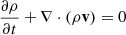 (A.1)
(A.1)
![Mathematical equation: $$ \begin{aligned} \frac{\partial \rho \mathbf v }{\partial t}&+ \nabla \cdot [\rho \mathbf v \mathbf v - \mathbf B B + \mathrm{I} (p + \frac{\mathbf{B ^2}}{2})] = \rho \mathbf g \end{aligned} $$](/articles/aa/full_html/2026/05/aa58324-25/aa58324-25-eq4.gif) (A.2)
(A.2)
 (A.3)
(A.3)
![Mathematical equation: $$ \begin{aligned} \frac{\partial E_t}{\partial t}&+ \nabla \cdot [(E_t + p_t) \mathbf v - \mathbf B (\mathbf v \cdot \mathbf B ) + \eta (\nabla \times \mathbf B ) \times \mathbf B ] \nonumber \\ &= \rho \mathbf v \cdot \mathbf g - \nabla \cdot \mathbf F_c - n^2 \Lambda (T) \, , \end{aligned} $$](/articles/aa/full_html/2026/05/aa58324-25/aa58324-25-eq6.gif) (A.4)
(A.4)
where ρ is the plasma density, p is the gas pressure, v and B are the velocity and magnetic fields. Et = ρv2/2 + ρe + B2/2 is the total energy density and pt = p + B2/2 the total pressure (gas pressure and magnetic pressure), e is the internal energy per unit mass. In these units, a factor  is included in the definition of the magnetic field B. The parameters η = 1 × 1011 cm2 s−1 and g = −G M⊙/R⊙2 ez = −27394 ez cm s−2 are the magnetic diffusivity and gravity at the solar surface, respectively. Both quantities are uniform and constant for the entire domain and the duration of the simulation.
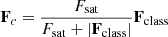
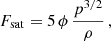
In Eq. (A.4), Fc is the thermal conduction flux, which varies between the classical (Spitzer-Härm) and saturated thermal conduction regimes Fclass and Fsat, respectively, and is given by:
 (A.5)
(A.5)
 (A.6)
(A.6)
 (A.7)
(A.7)
where b = B/B is a unitary vector parallel to the magnetic field, κ∥ = 5.6 × 10⁻⁷T5/2 erg s−1 K−1 cm−1, ϕ = 0.3. In our study, we only consider thermal conduction along the magnetic field. T corresponds to the plasma temperature and is given in Kelvin (K).
In Eq. (A.4), we also have the cooling term that depends on n, the density number, and Λ, the radiative loss function (Athay 1986) in the following form:
![Mathematical equation: $$ \begin{aligned} \Lambda = 10^{-22}&\{\ 0.4 \exp [-30 (\log T-4.6)^2] \\ &+ 4 \exp [-20(\log T-4.9)^2] \nonumber \\&+ 4.5\exp [-16(\log T-5.35)^2]\nonumber \\&+ 2\exp [-4(\log T-6.1)^2]\} \, , \end{aligned} $$](/articles/aa/full_html/2026/05/aa58324-25/aa58324-25-eq11.gif) (A.8)
(A.8)
where T is in K and Λ is in erg s−1. This formulation was used successfully in a global stellar wind model by Réville et al. (2020). It is not considered very precise at low temperature (typically below 104), but correctly reproduces the overall trend of the cooling rate as a function of temperature. It was used here for the sake of simplicity. More precise parametrisations, in particular for the chromosphere, will be used in future works (e.g. using CHIANTI, see Réville et al. 2024).
From Eq. (A.4), we can derive an equation for the evolution of the internal energy Eint = ρe = p/(Γ − 1), where Γ is the ratio of the specific heats cp/cv, as follows:
 (A.9)
(A.9)
where Fint = (p + Eint)v is the enthalpy flux. The second and third terms on the right-hand side correspond to the compression and advection components analysed in Sect. 3.1.
We solved the system of Eq. (A.1)–(A.4) in 3D cartesian coordinates using a 2nd order Runge-Kutta for advancing the solution in time, the Harten, Lax, Van Leer (HLL) approximate Riemann Solver and linear reconstruction. To preserve ∇ ⋅ B = 0, we consider the constrained transport method (Londrillo & del Zanna 2004; Gardiner & Stone 2005), where two sets of magnetic fields (face-centred and cell-centred) are used to calculate the electric field. We close the system using the perfect gas law with constant specific heat as an equation of state.
A.2. Grid
The computational domain spans ∓138 Mm in x with a total of 884 cells, from −124 to 62 Mm in y with 554 cells and from 0 to 186 Mm in the vertical direction z with 1024 cells. The grid spacing is uniform in x with a resolution of Δx = 312 km. In y and z directions the grid is mixed, having a uniform and stretched spacing. The horizontal y-coordinate is uniform, with Δymin = 312 km, in the area where the magnetic field is strong, in the range y = ∓62 Mm, comprising 398 cells. In the stretched part Δy increases to Δymax = 496 km in the region where the magnetic field is weak, from −62 to −124 Mm with 156 cells. For the vertical coordinate z, the spacing is uniform with Δzmin = 104 km in the lower atmosphere and beyond the transition region, from 0 to 10 Mm, comprising 96 cells, and is stretched in the corona, spanning from 10 Mm to 186 Mm with 928 cells resulting in Δzmax = 312 km. The stretched grid in PLUTO is defined as r (1 − rN)/(1 − r) = (xR − xL)/(Δx), where r is the stretching ratio, N is the number of points in the stretched grid, Δx is the uniform grid resolution and xL and xR are the leftmost and rightmost points of the stretched grid.
A.3. Initial conditions
We initialised the simulation using a plane-parallel stratified atmosphere together with a NFFF magnetic field extrapolation. For the magnetic field we applied a divergence cleaning method described by Valori et al. (2013), in which we correct the initial magnetic field B as 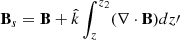 . This ensures ∇ ⋅ Bs = 0 to machine accuracy. Note that this correction only changes Bz, leaving the vertical component of the current density (∇×B)z unchanged.
Regarding the thermodynamical variables, we chose the density as a combination of two exponential functions:
![Mathematical equation: $$ \rho = \rho _1\exp \left[\frac{-(z - z_{ch})}{z_{c1}}\right] + \rho _2\exp \left[\frac{-(z - z_{ch})}{z_{c2}}\right] \, . $$](/articles/aa/full_html/2026/05/aa58324-25/aa58324-25-eq14.gif)
The values chosen for this simulation were ρ1 = 4 × 10⁻¹⁰ g cm−3, ρ2 = 1.67 × 10⁻¹³ g cm−3, zch = 0.075 Mm, zc1 = 0.25 Mm and zc2 = 30 Mm. This gave density values ranging from 3 × 10⁻¹⁶ to 3 × 10⁻¹⁰ g cm−3, and from 3 × 10⁻² to 300 dyn cm−2 for the gas pressure.
From the hydrostatic equilibrium equation we obtained the profile for the gas pressure. The temperature T is defined with the thermal equation of state p = kB ρ T/mu μ, where kB is the Boltzmann constant, mu is the atomic mass unit and μ the mean molecular weight. We assumed that the plasma is fully ionised (μ = 0.5). We obtained that the temperature varies from 4 × 10³ to 5 × 10⁵ K. Fig. A.1 summarises different initial variables as a function of height. Panel a) displays the temperature (red solid line) and the density (green solid line). Panel b) displays the gas pressure (blue) together with the horizontal average of the plasma β (black). The light-grey area around < β> H spans from the minimum value of plasma-β (bottom limit) to the maximum value (upper limit) at each height. The amplitude of these values shows the non-uniformity of this parameter, especially below the transition region (located at z ≈ 1 − 2 Mm), being < β> H < 1 above 7 Mm and entirely lower than one above 70 Mm. The large values of β below the corona (z < 3 Mm) correspond to small localised regions in the quiet Sun, in opposite directions where the eruption will develop. Panel c) exhibits the variation of the horizontal average of the Lorentz force norm with height (black) together with the gas pressure gradient in the vertical direction (blue) and the gravity force (dashed yellow). The vertical dashed grey lines in all the panels show the limit where we used a uniform grid (to the left of this line) and a stretched grid (to the right) in z.
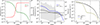 |
Fig. A.1. Vertical initial profiles. a) Density (ρ, green solid line) and temperature (T, red solid line) as function of height. b) Gas pressure (p, blue solid line) and horizontal average of plasma β (< β> H, black solid line). The grey area covers the minimum and the maximum values of β for each height. The horizontal grey line indicates β = 1. c) Initial forces: horizontal average of the vertical Lorentz force (< LFz> H, black solid line), gas pressure gradient ((∇p)z, blue solid line) and gravity (ρg, dashed yellow line). The vertical dashed grey line indicates the division between uniform and stretched grid in z. |
Figure A.2 shows the initial magnetic field obtained from the NFFF extrapolation. Panel a) shows the vertical component Bz at the z = 0.05 Mm and the dashed-red line delimits the region where the grid is uniform in y (above the red line) and stretched (below it). Note that the active region is not centred with the y-coordinate of the simulation box. The reason of this choice is that, from observations, the eruption is ejected towards the south (negative y in our simulation box), thus we only extended the domain in this direction to maximise numerical efficiency. Panel b) shows the magnitude of the magnetic field in grey scale in two perpendicular planes at around y = −7 Mm and x = −15 Mm and panel c) shows a 3D view of the magnetic field (thin magenta lines) together with the field lines that will form the flux rope (thick magenta lines).
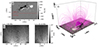 |
Fig. A.2. Initial magnetic field. a) Initial Bz at z = 0.05 Mm in grey scale, positive (negative) values are in white (black). The dashed red line indicates the division between the uniform and stretched grid in y. b) Cuts on vertical planes at y = −7.63 Mm (left) and x = −15.14 Mm (right). The magnitude of the magnetic field is shown in grey scale and the black lines correspond the streamlines of the projected magnetic field vector on each plane. c) 3D visualisation of B (thin magenta lines), with the flux rope field lines highlighted (thick magenta lines). |
A.4. Boundary conditions
For the bottom boundary, we used the line-tied conditions expressed by Aulanier et al. (2005), in which all the components of the velocity are set to zero for the entire duration of the simulation, meaning that vxi, j, KBEG = vyi, j, KBEG = vzi, j, KBEG = 0, where KBEG corresponds to the first index of the physical domain in the vertical coordinate z, i = IBEG, ..., IEND and j = JBEG, ..., JEND corresponds to the horizontal coordinates x and y, respectively. For the ghost cells we defined symmetry for ρ and antisymmetry for vz that proved to be efficient at enforcing line-tying (e.g. Aulanier et al. 2005) as:


where k = 1, 2. The third index on the left hand side spans the two ghost cells and the one in the right hand side extends over the physical domain. For all the remaining variables, we defined second derivative centred at KBEG to be zero (linear extrapolation), resulting in:

where f = {p, vx, vy, Bx, By, Bz}.
For the side boundaries, we set zero-gradient conditions for ρ, p and v, fixing to zero the normal component of velocity in case it goes inwards, to avoid having inflows. For the magnetic field, we considered linear extrapolation with centred derivative at IBEG and IEND for the planes yz as follows:


where i = 1, 2. For the xz planes, we used:


where j = 1, 2. The asymmetry in this condition is due to the end boundary in the y-direction is still close to the centre of the active region, as it was not extended as much as in the other y-direction in order to minimise the numerical cost of the simulations. When using a linear extrapolation for the magnetic field there, we found that spurious inflows could form and affect this part of the simulation domain (while not affecting the eruption under study here itself, as it happens on the other side of the active region). Still, to avoid these spurious boundary effects we found that using a zero-gradient boundary condition on this side of the box prevented the simulation from exhibiting any discernible effect from this lateral boundary. We kept these conditions for the magnetic field on the sides until the shock caused by the initial instability has left the domain, which is around t = 4.20 min. After that time, we used the zero-gradient for B for all the side boundaries.
For the top boundary, we applied zero-gradient for ρ, p, vx, vy and vz, setting vz = 0 if it is pointing inward. For Bx, By and Bz we applied linear extrapolation.
Appendix B: GUITAR
GUITAR is a graphical user interface designed to extract flux rope field line source points from 2D flux rope proxy maps (Wagner et al. 2024c). Commonly-used thresholds like the twist number 𝒯w or the winding number 𝒯g can serve as proxy for the location of magnetic flux ropes (see e.g. the appendix in Liu et al. 2016, for an extensive discussion on these twist metrics). However, often this is not a sufficient criterion as multiple twisted structures in simulation data may be present. To improve the results of a thresholding procedure, GUITAR incorporates mathematical morphology algorithms namely dilatation and erosion. These are built upon comparing image elements with a pre-defined shape with variable size called the structuring element (SE).
We applied these algorithms to thresholded 𝒯w maps. More precisely, we used a binary formalism of them. Let X be a binary image. The selected region, called C, corresponds to values 1 within X (which are not necessarily connected), and SE is the structuring element with centre point s. Then the dilation of X (X ⊕ SE) is the union of all points x ∈ X that the SE can reach, with SE centred at any point c ∈ C. Thus, the dilation operation adds values 1 at the edges of C, depending on the shape and size of SE. On the other hand, the erosion of X (X ⊖ SE), is the union of all centre points s of the SE for which SE is fully contained in C. Thus, the erosion operation removes values 1 at the edges of C, depending on the shape and size of SE. Note these algorithms are (in most cases) not inverse to each other and combining them in particular ways results in very useful new procedures.
Most notably, for the applications in GUITAR, the opening algorithm corresponds to the dilation of an erosion: (X ⊖ SE) ⊕ SE. It is typically used to remove noise or unwanted (sub-)features. This is particularly useful for post-processing the thresholding of 𝒯w (or other flux rope proxy) maps. A circle is selected for SE in the case of GUITAR, to avoid the flux rope cross section to contain sharp edges in regions where processing is applied. Once the user is satisfied with the results, the desired feature can be tracked through time. Lastly, the source points can be saved either via uniform or random sampling within the extracted binary shapes. Finally, it should be noted that GUITAR is also designed to customise and save plots and animations, export intermediate steps during the processing and do a basic 2D analysis of the time series of the extracted binary shapes, for example, the flux rope cross-section (Wagner et al. 2024c).
Appendix C: Magnetic reconnection
To inspect the presence of magnetic reconnection in the simulation, we computed the squashing factor Q, which measures the deformation of the field line mapping between two surfaces. The regions where the gradients in the mapping are large are referred as quasi-separatrix layers (QSLs), and are a continuous extension of separators and separatrix surfaces. These QSLs are potential sites for the formation of strong electric currents and, therefore, possible regions where magnetic reconnection can occur. For the calculations of Q we used the package K-QSL4 which follows the method described in Scott et al. (2017) and Tassev & Savcheva (2017). The results of sign(Bz)log(Q) for a cutting plane at x = 5 Mm and at different times are shown in Fig. C.1. High values of Q are denoted in orange (for Bz > 0) and dark purple (for Bz < 0). The field lines corresponding to the flux rope are displayed in magenta. The black ellipses highlight the regions where the flux rope field lines cross through areas of high Q, suggesting that these field lines are reconnecting. The times considered in this figure correspond to a stage before the triggering of the rising phase (t = 1.91 min), at the beginning and during it (t = 3.43 min and t = 4.96), and for a later time where there is a clear increase of the vertical velocity of the flux rope (t = 6.11 min, see panel c) from Fig. 9 as a reference).
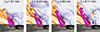 |
Fig. C.1. Early evolution of the squashing factor Q. The panels display sign(Bz)log(Q) for a cutting plane at x = 5 Mm in purple (negative Bz) to orange (positive Bz) colours for t = 1.91 min, t = 3.43 min, t = 4.96 min, and t = 6.11 min. The magenta lines correspond to the flux rope field lines. The black ellipses indicate regions of intersection of the field lines with high Q values areas. |
Appendix D: Force Analysis
To complement the analysis discussed in Sect. 4, in Fig. D.1 we show the forces that contribute to the net force displayed in Fig. 9. We excluded gravity in the figure because it is almost negligible compared to the other forces. These forces correspond to each term of the divergence operator (whose signs are as if they were on the right hand side of the equation) and the source term of Eq. (A.2). The columns indicate the simulation time (which is the same as in Fig. 9) and the rows represent the different forces in the vertical direction z in blue (negative) to red (positive values). Panels a) to e) show the vertical component of the Lorentz force (LFz), f) to j) exhibit the negative vertical component of the gas pressure gradient (−(∇p)z), the net contribution between these two (LFz − (∇p)z) is shown in panels k) to o) and in panels p) to t) the contribution of the advection term (−(v ⋅ ∇)vz).
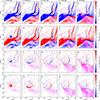 |
Fig. D.1. Evolution of the vertical forces (positive values are in red and negative values in blue) at z = 24 Mm for t = 4.5 min, t = 4.96 min, t = 6.11 min, t = 7.63 min and t = 8.78 min. Panels a) to e) show the vertical component of the Lorentz force, f) to j) display the negative gas pressure gradient, k) to o) exhibit the net contribution of the Lorentz force and gas pressure gradient and panels p) to t) the advective component of the force. The magenta lines represent flux rope magnetic field lines, the darker (lighter) segments of the lines are above (below) the cutting plane. Grey contours indicate positive (solid) and negative (dashed) values of Bz at z = 0.05 Mm and the green contours exhibit different values of vz between 218 (dark green) and 436 km s−1 (light green). |
The contribution of the Lorentz force is always negative in the region where we have higher vz (green contour), which is near the region where the magnetic field lines are emerging the cutting plane, except for t = 4.50 min. The opposite happens with the pressure gradient force −(∇p)z, where we find positive contribution in the high speed regions. These two forces mostly cancel each other as shown in panels k) to to o). In the region of higher vertical velocity (within and nearby the dark green contour), the net contribution is first negative (panels k) and l)), then positive (panels n) and o)). This indicates that the contribution of the gas pressure gradient is slightly larger than that of the Lorentz force.
Regarding the advection, panels p) to t), its contribution to the source term of Eq. (A.2) is positive for the gradual expansion phase, from t = 4.50 to t = 4.96 min, and negative for the rising phase, from t = 6.11 to t = 8.78 min. Since the total force is positive (within and nearby the dark green contour), as shown in Fig. 9, the Eulerian increase of velocity is first mainly due to the convective transport from below, and then to the pressure gradient force.
All Figures
|
Fig. 1. Active region NOAA 12241. a) Full-disk image in 171 Å observed by SDO/AIA on December 18, 2014, at 21:24 UT. The blue rectangle indicates the active region under study. b) Zoom-in of the active region in 171 Å. c) LOS magnetogram taken by SDO/HMI. The red rectangle indicates the horizontal domain for the numerical simulation. |
| In the text | |
|
Fig. 2. Initialisation and evolution of the eruption at a glance. In all the panels, a magnetogram, with white to black levels, is present in the background to make the link with observations in Fig. 1. The colour map is saturated between −400 and 400 G for visualisation purposes. a) Initial magnetic configuration and Lorentz force at t = 0 s. The pink lines represent the magnetic arcade that was later on transformed into the erupting flux rope. The green to yellow colour map indicates a volumetric representation of the magnitude of the Lorentz force; yellow (green) is more (less) intense. b) Zoom-in at t = 0.23 s of the region defined by the grey rectangle in panel a. The horizontal components of the Lorentz force are shown with arrows in blue (negative) and red (positive), drawn at a height z = 2.2 Mm. Temperature iso-surfaces of 2 × 10⁶ K (red) to 4 × 10⁶ (yellow) are also displayed. c) Rising phase for t = 6.87 min, t = 9.92 min, and 12.59 min. The coloured lines represent the magnetic field lines corresponding to the flux rope. The colour of the field lines represents the vertical speed vz in pink. The two lines in the xy-plane indicate the cuts where the tracking (T line in light turquoise) of the flux rope and the compression (C line in dark turquoise) analysis were performed. |
| In the text | |
|
Fig. 3. Thermodynamical variables in the rising phase. a) Density and b) temperature at x = 5 Mm (corresponding to line T in Fig. 2c) for t = 12.59 min. Yellow denotes higher density and temperature, and blue shows lower values. The solid white lines represent the streamlines of the projected magnetic field vector on the plane. A movie showing the temperature in this cutting plane together with 3D visualisation of the flux rope field lines is available in the online version. |
| In the text | |
|
Fig. 4. Kinematic properties of the flux rope apex. We show the vertical coordinate of the flux rope apex at x = 5 Mm (blue dots) and quadratic fit (solid orange line). The values of the vertical velocity are added at different times. Before t = 4 min, the flux rope is not sufficiently well formed to infer the apex height. |
| In the text | |
|
Fig. 5. Evolution of energies averaged in the entire computational domain. The total energy is shown as the solid black line, the total magnetic energy is shown as the solid blue line, the free magnetic energy is shown as the dashed blue line, and the kinetic and internal energies are shown as solid orange and green lines, respectively. The vertical dotted lines indicate different stages. |
| In the text | |
|
Fig. 6. Lorentz force and energy source terms for the plane x = −15 Mm (see its photospheric trace C in Fig. 2). a) Lorentz force on the y-axis at t = 0 s (positive values are shown in red, and negative values are shown in blue), b) compression, c) advection, and d) radiative cooling at t = 0.23 s (positive values are indicated in dark orange, and negative values are shown in purple). The upper limit of the transition region is denoted with the solid black line. |
| In the text | |
|
Fig. 7. Evolution of thermodynamical variables along a magnetic field line. a) We show the plane-of-sky coordinates of a magnetic field line, represented with dotted (t = 0 s), dashed (t = 0.23 s), dash-dotted (t = 1.14 s), and solid lines (t = 13.74 s), from light to dark pink. In the background, Bz at z = 0.05 Mm and t = 0 s is shown in greyscale, with negative values in black and positive values in white. b) Temperature. c) Vertical velocity along the field line from the left footpoint to the apex (top panels) and from the right footpoint to the apex (bottom panels). The variables are plotted for the same instants in time as in panel a. |
| In the text | |
|
Fig. 8. Twist 𝒯w at x = 5 Mm (cut T in Fig. 2) for a) t = 7.63 min, b) t = 8.78 min, and c) t = 9.92 min. Pink indicates positive values of twist related to a current density parallel to the magnetic field for the corresponding field line, and green denotes the anti-parallel orientation. The grey circles represent the points belonging to the flux rope extracted with GUITAR. |
| In the text | |
|
Fig. 9. Top panels: Evolution of the net vertical force (positive values are plotted in red, and negative values are shown in blue) at z = 24 Mm for a) t = 4.5 min, b) t = 4.96 min, c) t = 6.11 min, d) t = 7.63 min, and e) t = 8.78 min. The magenta lines correspond to field lines computed within the flux rope. The grey contours indicate positive (solid) and negative (dashed) values of Bz at z = 0.05 Mm, and the green contours exhibit different values of vz between 218 (dark green) and 436 km s−1 (light green). Bottom panels: Flux rope magnetic field lines in 3D coloured by vz for the same times as in the top panels. The semi-transparent grey plane corresponds to z = 24 Mm and contains the same vz contours as the top panels. |
| In the text | |
|
Fig. 10. Evolution of the magnetic pressure at z = 60 Mm for (a) t = 7.63 min, (b) 8.78 min, and (c) t = 9.92 min. The background colour shows the variation in B2/8π in a blue-to-yellow colour map, with blue being the lowest and yellow the highest value. The different field lines displayed in magenta correspond to the apex and to the left and right flanks of the flux rope. The contours show different values of β of 0.1 (indigo), 1 (white), and 10 (yellow). |
| In the text | |
|
Fig. A.1. Vertical initial profiles. a) Density (ρ, green solid line) and temperature (T, red solid line) as function of height. b) Gas pressure (p, blue solid line) and horizontal average of plasma β (< β> H, black solid line). The grey area covers the minimum and the maximum values of β for each height. The horizontal grey line indicates β = 1. c) Initial forces: horizontal average of the vertical Lorentz force (< LFz> H, black solid line), gas pressure gradient ((∇p)z, blue solid line) and gravity (ρg, dashed yellow line). The vertical dashed grey line indicates the division between uniform and stretched grid in z. |
| In the text | |
|
Fig. A.2. Initial magnetic field. a) Initial Bz at z = 0.05 Mm in grey scale, positive (negative) values are in white (black). The dashed red line indicates the division between the uniform and stretched grid in y. b) Cuts on vertical planes at y = −7.63 Mm (left) and x = −15.14 Mm (right). The magnitude of the magnetic field is shown in grey scale and the black lines correspond the streamlines of the projected magnetic field vector on each plane. c) 3D visualisation of B (thin magenta lines), with the flux rope field lines highlighted (thick magenta lines). |
| In the text | |
|
Fig. C.1. Early evolution of the squashing factor Q. The panels display sign(Bz)log(Q) for a cutting plane at x = 5 Mm in purple (negative Bz) to orange (positive Bz) colours for t = 1.91 min, t = 3.43 min, t = 4.96 min, and t = 6.11 min. The magenta lines correspond to the flux rope field lines. The black ellipses indicate regions of intersection of the field lines with high Q values areas. |
| In the text | |
|
Fig. D.1. Evolution of the vertical forces (positive values are in red and negative values in blue) at z = 24 Mm for t = 4.5 min, t = 4.96 min, t = 6.11 min, t = 7.63 min and t = 8.78 min. Panels a) to e) show the vertical component of the Lorentz force, f) to j) display the negative gas pressure gradient, k) to o) exhibit the net contribution of the Lorentz force and gas pressure gradient and panels p) to t) the advective component of the force. The magenta lines represent flux rope magnetic field lines, the darker (lighter) segments of the lines are above (below) the cutting plane. Grey contours indicate positive (solid) and negative (dashed) values of Bz at z = 0.05 Mm and the green contours exhibit different values of vz between 218 (dark green) and 436 km s−1 (light green). |
| In the text | |
Current usage metrics show cumulative count of Article Views (full-text article views including HTML views, PDF and ePub downloads, according to the available data) and Abstracts Views on Vision4Press platform.
Data correspond to usage on the plateform after 2015. The current usage metrics is available 48-96 hours after online publication and is updated daily on week days.
Initial download of the metrics may take a while.