


| Issue |
A&A
Volume 709, May 2026
|
|
|---|---|---|
| Article Number | A257 | |
| Number of page(s) | 17 | |
| Section | Interstellar and circumstellar matter | |
| DOI | https://doi.org/10.1051/0004-6361/202556500 | |
| Published online | 27 May 2026 | |
A complete X-ray view of supernova remnant W28 with the Einstein Probe: Spatial distribution of parameters, and the origin of the thermal-composite morphology
1
School of Astronomy and Space Science, Nanjing University,
Nanjing
210023,
China
2
Key Laboratory of Modern Astronomy and Astrophysics, Nanjing University, Ministry of Education,
Nanjing
210023,
China
3
Department of Astronomy, Tsinghua University,
Beijing
100084,
China
4
State Key Laboratory of Particle Astrophysics, Institute of High Energy Physics, Chinese Academy of Sciences,
Beijing
100049,
China
5
Department of Astronomy, Xiamen University,
Xiamen,
Fujian
361005,
China
6
National Astronomical Observatories, Chinese Academy of Sciences,
Beijing
100012,
China
★ Corresponding author: This email address is being protected from spambots. You need JavaScript enabled to view it.
Received:
18
July
2025
Accepted:
17
March
2026
Abstract
The question about what causes a supernova remnant (SNR) to be a thermal composite rather than have a typical shell-like morphology remains unsolved, as does what causes the plasma inside it to recombine. With the 13-ks observation of the Following-up X-ray Telescope on board the Einstein Probe, we give an overall X-ray picture of W28, one of the prototypical thermal composite SNRs. The observation revealed a shell-like structure west of W28 in radio, optical, and X-ray images. This may revise the known extent of the SNR to 72′ × 45′. A spectral analysis explicitly maps the special relation in which the plasma experiences recombination in the interior of the remnant, spatially coincident with Hα emissions, while in other regions, the plasma is dominated by ionization. We found that W28 is generally isobaric from its center to the newly discovered shell, and it is even isothermal with a temperature of ∼0.6-0.7 keV in the center before the plasma cools. Saturated thermal conduction and cloud evaporation may cool down the plasma within ∼3 kyr, which is the estimated recombination timescale. We revised the SNR dynamical age to ∼8 kyr, which is much younger than previous estimates. The complex structure and complex ionization state distribution may suggest that centrally filled and shell-like morphologies coexist in W28. This state may depend on the environment in which the SNR evolves.
Key words: plasmas / ISM: supernova remnants / X-rays: ISM
© The Authors 2026
 Open Access article, published by EDP Sciences, under the terms of the Creative Commons Attribution License (https://creativecommons.org/licenses/by/4.0), which permits unrestricted use, distribution, and reproduction in any medium, provided the original work is properly cited.
This article is published in open access under the Subscribe to Open model. This email address is being protected from spambots. You need JavaScript enabled to view it. to support open access publication.
1 Introduction
Supernova remnants (SNRs) are important extended objects that are mainly shaped by the interaction between supernova (SN) shocks and ambient gas, including the interstellar medium (ISM) in the environment and circumstellar medium (CSM) created by the stellar winds of the progenitor. The rapid shock of the SN can effectively compress, heat, and finally sweep the gas into a thin bright shell, which is the canonical morphology of SNRs and is well expected by self-similar models such as the Sedov-Taylor solution (Sedov 1959; Taylor 1950) and the Chevalier self-similar model (Chevalier 1982). The shock can also effectively accelerate particles to GeVs or even tens of TeVs, leading to synchrotron emissions from radio to X-rays on the shell. In addition to the shocked gas, neutron stars created in core-collapse SNe can also prominently contribute to the total luminosity of the SNR, with nonthermal emissions of their relativistic electron/positron plasma, or rather the pulsar wind nebula (PWN). The most representative example of PWN-dominated SNR (or filled center or plerion) is the Crab nebula. Composite SNRs are also expected when the shell and PWN are both observable. Examples include G11.2-0.3, G292+1.8, and Kes 75.
In addition to the three morphologies mentioned above (shell-like, plerion, and composite), one new classification of SNR, thermal-composite (or mixed-morphology) SNRs, was later discovered based on the development of X-ray astronomy. An archetype of these SNRs is W28 (SNR G6.4–0.1) at a distance of ∼ 1.9 kpc (Velázquez et al. 2002). It is characterized by a centrally filled X-ray and shell-like radio morphology (Rho & Petre 1998). Additionally, OH masers (Frail et al. 1994; Claussen et al. 1997; Hoffman et al. 2005), molecular clouds (Arikawa et al. 1999; Velázquez et al. 2002; Reach et al. 2005; Mazumdar et al. 2022), and GeV-TeV γ-ray emissions probably with a hadronic origin (Rowell et al. 2000; Aharonian et al. 2008; Abdo et al. 2010; Li & Chen 2010; Cui et al. 2018) are associated with W28, with a proposed age of ∼33-42 kyr (Rho & Borkowski 2002; Velázquez et al. 2002; Li & Chen 2010). X-ray observations toward the SNR center revealed that the electron temperature (measured from the bremsstrahlung continuum) is lower than the ionization temperature (reflected by the ionization state of heavy elements), meaning that the recombining process of ions dominates ionization (Sawada & Koyama 2012). This overionized or recombining nonequilibrium ionization (NEI) may suggest the plasma has experienced a cooling process from a high temperature (Itoh & Masai 1989; Kawasaki et al. 2005; Yamaguchi et al. 2009; Pannuti et al. 2017; Okon et al. 2018; Himono et al. 2023) or other mechanisms such as photoionization (Ono et al. 2019).
Some theoretical models were proposed to explain the unique morphology of thermal-composite SNRs. For very mature SNRs experiencing radiative loss, the cool shell would be invisible in X-rays due to absorption (Rho & Petre 1998). Other scenarios generally require a high-density environment with density gradients, including evaporation of cloudlets engulfed by the shock (White & Long 1991), thermal conduction in the interior hot gas (Cox et al. 1999; Shelton et al. 1999), shocks reflected from a cavity wall (Chen et al. 2008), and a projection effect of an asymmetric shell of shocked CSM (Shimizu et al. 2012). For a comparison, the Sedov-Taylor solution assumes the evolution in a uniform medium.
However, a complex environment with a density gradient may suggest different dynamical evolutions in different directions. In this case, a classification of SNRs might be expected as the transition between the shell-like and the thermal-composite, some part of which evolves in the normal ISM, while the other part interacts with dense clouds. On the other hand, thermalcomposite SNRs are commonly medium-age objects, but their early-stage evolution is not yet clear. In particular, a great number of nearby X-ray-bright SNRs with large angular sizes (≳1°) have a thermal-composite X-ray morphology (Ferrand & Safi-Harb 2012), such as HB 3 (Lazendic & Slane 2006), HB 9 (Sezer et al. 2019), HB 21 (Lazendic & Slane 2006), W63 (Mavromatakis et al. 2004), and G65.3+5.7 (Shelton et al. 2004).
To understand the centrally filled X-ray morphology of thermal composite SNRs, we need to map the properties of the shocked hot gas via a spatially resolved X-ray analysis of an entire SNR. However, current X-ray observation missions like Chandra (Weisskopf et al. 2002), XMM-Newton (Jansen et al. 2001), and Suzaku (Mitsuda et al. 2007) are limited by their small field of view (17′-30′). It is time-consuming to mosaic SNRs with a large angular size, and multiple-pointing observations make handling the spatially varying response and instrumental effect a great challenge. For W28, for instance, previous studies (Rho & Borkowski 2002; Kawasaki et al. 2005; Sawada & Koyama 2012; Zhou et al. 2014; Nakamura et al. 2014; Pannuti et al. 2017; Okon et al. 2018; Himono et al. 2023) mainly focused on the W28 center, on clump D (previously called southwestern shell; Rho & Borkowski 2002), and on the NE shell (see the labels in Fig. 1). Our new study covers the vicinity of these bright structures, which enabled us to search for a possible further extension of this remnant.
We present the first spatially resolved spectral analysis of the entire W28 based on the Follow-up X-ray Telescope (FXT; Chen et al. 2020, 2025), which is one of the two science instruments on board the Einstein Probe (EP; also named “Tianguan”; Yuan et al. 2022), which launched on January 9, 2024, in Xichang, China. The FXT consists of two co-aligned Wolter-I modules, FXTA and FXTB. With a large field of 1° × 1°, a total effective area of ∼600 cm2 at 1 keV, and a low instrumental background at a level of ∼4 × 10⁻³ counts s−1 cm−2 keV−1 in 0.3-10 keV (Zhang et al. 2022), FXT has the powerful capability of observing very diffuse X-ray sources such as SNRs, superbubbles, the Galactic ridge, and galaxy clusters. Despite its short exposure, FXT provides a brand-new view of this famous SNR. Long-exposure XMM-Newton data were used as supplementary and verification in our study.
This paper is organized as follows: we present the process of EP-FXT and XMM-Newton data in Sect. 2. The morphology and spectroscopy analysis are shown in Sects. 3.1 and 3.2. Then, we discuss our results in Sect. 4 and summarize this paper in Sect. 5.
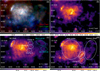 |
Fig. 1 Energy-coded X-ray image of the W28 complex with FXT (a), consisting of bands in 0.4-0.7 keV (red), 0.7-1.1 keV (green), and 1.12.3 keV (blue). The single-band images of each energy band are shown in panels (b), (c), and (d). The images are in units of count s−1 cm−2 and in a square-root color scale to enhance weak emissions. All the images are vignetting-corrected and adaptively smoothed. The structures mentioned in this paper are marked in panels (c) and (d). The cyan regions correspond to optical and/or radio SNR candidates (Stupar & Parker 2011; Stupar et al. 2018). |
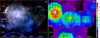 |
Fig. 2 (a) Same as Fig. 1a but based on XMM-Newton data. The arc-like patterns of the stray light from GX 5-1 are visible in the south, marked between dashed white lines. (b) Effective exposure time of XMM-Newton in units of ks scaled as MOS2 with the Medium filter, which shares a similar effective area with one FXT module. |
2 Data reduction
2.1 EP-FXT
W28 was proposed to verify the imaging spectroscopy ability of FXT in the performance verification (PV) phase from April to May 2024. The observational program consists of two individual pointing observations in Full-Frame mode with the Thin filter (for detailed technical information of FXT, see the instrument webpage1 and the user guide2), and the total coverage sky area is 1.5° × 1°. The detailed information is listed in Appendix A.
The FXT observations are reprocessed by the Follow-up X-ray Telescope Data Analysis Software (FXTDAS3) with the standard reprocessing threads including scripts fxtcoord, fxtpical, fxtparticleidentify, fxtcoord, fxtbadpix, fxthotpix, fxtgrade, and fxtgtigen. In these processes, the bad events from bad, hot, and flickering pixels, cosmic rays, and bad time intervals are removed. Energy- and coordinate-calibrated events are then reconstructed (for details, see Chi et al., in prep.). Only events flagged with status=0 and pattern≤12 were used for analysis. The event lists of two observations were reprojected and combined.
Images of selected energy bands were extracted with the FTOOLS (Blackburn 1995) script ftcopy from the reprojected event file. The task fxtexpogen creates exposure maps for vignetting correction and masking pixels with RAWY<20 to avoid the shadow of the frame storage area. The exposure maps were combined regarding the effective area of FXTA and FXTB, and the vignetting-corrected image was adaptively smoothed with the dmimgadapt script in the Chandra Interactive Analysis of Observations (CIAO, version 4.16; Fruscione et al. 2006) package. The vignetting-corrected and adaptively smoothed images of W28 are shown in Fig. 1.
The spectra of the regions defined by polygons were extracted with Xselect and then grouped with grppha to guarantee a minimum signal-to-noise ratio of 3 per bin. The response files were generated with fxtarfgen and fxtrmfgen. XSPEC (version 12.14.a; Arnaud 1996) based on AtomDB (version 3.0.9; Foster et al. 2012) was used for the spectral fitting.
2.2 XMM-Newton
We also retrieved archival XMM-Newton data of W28. Compared to FXT, XMM-Newton has a slightly higher angular resolution and a higher throughout, especially in the W28 NE shell. The region of interest in our study consists of 13 different pointings with a total exposure of ∼186 ks for an overall but not uniform coverage (see Appendix A and Fig. 2), most of which belong to large programs such as the XMM-Newton Galactic Plane Survey (Hands et al. 2004). This made the background estimation and response weighting for the spectral analysis difficult. Hence, we mainly used XMM-Newton for imaging here and used the NE shell of W28, which has the deepest XMM-Newton exposure, as a spectral calibrator to verify the performance of FXT (see Appendix B for details).
The XMM-Newton data were processed and analyzed with the XMM-Newton Science Analysis Software (SAS version 20.0; Gabriel et al. 2004) and the XMM-Newton Extended Source Analysis Software (ESAS) package with the latest calibration files. The MOS (Turner et al. 2001) and pn (Strüder et al. 2001) observations were calibrated with emchain and epchain, and then filtered the high-level background with mos-filter and pn-filter, respectively. We realized that XMM-Newton observation 0886110701, whose nominal point is in the southwest of W28, was coincidentally applied on the same day as the FXT observations. With a long exposure of ∼20 ks, it can also play the role of a flare monitor for FXT, which shows a low smooth sky background count-rate level.
Imaging and spectral extraction were based on threads mos-spectra and pn-spectra. The instrumental background or quiescent particle background (QPB) images and spectra were modeled by mos_back and pn_back. The images were then mosaicked via merge_comp_xmm and then adaptively smoothed by adapt_merge.
 |
Fig. 3 Tricolor image of W28 in the radio (red, 1.3 GHz continuum), Hα (green), and X-ray (blue, 0.4-2.3 keV) bands. A square root color scale is used to highlight faint diffuse emissions in the radio and X-ray images. The white polygon regions are used for spectral extraction and analysis, and the dashed cyan regions correspond to the sky background. The yellow contours correspond to the MWISP CO intensity in the –20-10 km s−1 (Tu et al. 2024). The optical nebulae southeast and northeast of W28 are the Lagoon Nebula Messier 8 and the Trifid Nebula Messier 20, respectively. |
2.3 Optical and radio data
Optical and radio data were used to reveal the multiwavelength morphology of W28. We retrieved narrowband Hα images of the AAO/UKST SuperCOSMOS Hα survey with an angular resolution of ∼1" (Parker et al. 2005). To underline the morphology of Hα-emitting gas from the starlight continuum, the R-band images were used to make an Hα∕R ratio map. In the radio, the SARAO MeerKAT 1.3 GHz Galactic Plane Survey (Goedhart et al. 2024) that covers areas of |b| ≤ 1.5° provides complete coverage of W28 along with its environment with an angular resolution of ∼8″.
3 Results
3.1 Morphology
Figures 1 and 2 show the X-ray morphology of W28. The centrally filled plasma with a radius of ∼15′ (or W28 center hereafter, defined in Fig. 1) dominates X-ray emissions of the entire SNR, which is the canonical feature of thermal-composite SNRs. The X-ray luminosity peaks in the center, and there are no evident asymmetric structures such as jets or bars. Two clumpy structures (Clumps D & E; southwestern shell in Rho & Borkowski 2002) are enhanced above 1.1 keV in the southwest. The northern structure, clump D, appears to be brighter in the hard X-ray band. Either a strong foreground absorption or a high temperature may account for this feature.
Previous studies (Long et al. 1991; Zhou et al. 2014; Nakamura et al. 2014; Pannuti et al. 2017; Okon et al. 2018; Himono et al. 2023) focused on the center, the northeastern shell, and the brighter clump in the southwest. However, FXT reveals a much more extended X-ray morphology than before. Two shell-like X-ray structures (collectively named “western shell” hereafter) are evident west of the W28 center, whose extension is comparable to the diameter of the center. This structure is spatially coincident with radio and optical filaments in the multiwavelength image (Fig. 3). A morphology like this is typically formed by shock interaction with the ISM and is common in SNRs. Noticeably, the northern part of this western shell was reported as part of an undiscovered SNR (G6.31+0.54 therein), diagnosed by an enhanced [S II]/Ha ratio (Stupar et al. 2018). On the other hand, its central part was proposed to be a Galactic SNR G6.10+0.53 according to the Hα image and radio spectral index (Brogan et al. 2006; Stupar & Parker 2011). Here, the FXT image provides further evidence for its SNR origin through the spectral analysis (see the subsection below). Without a complete shell, the western shell could be part of W28 based on its curvature and orientation. A similar morphology appears in the famous thermal-composite SNR IC 443, whose western shell, located farther away, is fainter and larger than its eastern shell.
In addition, three X-ray-emitting clumps (clumps A, B, and C, or regions 5, 6, and 8 in Fig. 3) appear west of the center aligned from north to south, and share a similar size, ∼6′ in diameter, apparently outside the bright radio shell. Clumps A and B are located beyond the radio shell, and the Hα emissions there do not show filamentary structures in shocked regions like the NE shell and the western shell.
In the east, diffuse X-ray emissions (region 46) are visible near a radio ring, which was considered an independent SNR, G6.5–0.4. However, the X-rays appear south of the radio emissions. Therefore, the morphology alone cannot determine whether the X-ray emissions here originate from G6.5–0.4 or W28. A point-like source (RA=18:02:00, Dec=–23:42:00 in Fig. 1d) with a diffuse X-ray halo around it appears south of the eastern X-ray emissions. These features are spatially associated with an O6III blue giant in an HII region according to the SIM-BAD database (Wenger et al. 2000). Related optical and radio emissions can be seen in Fig. 3 as well.
3.2 Spectroscopy
We manually divided emissions associated (or overlapping) with W28 into 46 polygon regions (see Fig. 3) for spectrum extraction. The definition of a region mainly depends on its morphology to guarantee a uniform distribution of its X-ray surface brightness and the total photon numbers (a smaller area for a brighter region). In addition, the region boundaries were limited within the field of view in order to make full use of the observed X-ray photons. The spatial sampling rate declines from the center to the edge to balance the spectral quality and spatial resolution of the spectral analysis. We directly subtracted the sky background (dashed cyan ellipse in Fig. 3) from the source spectra, as W28 is bright enough (one to two orders of magnitude higher than the sky in 1-2 keV) and the sky background is difficult to model for the short exposure.
The challenge for a spectral analysis is the contamination of stray light, or rather, that the X-ray photons experience only one reflection from an off-axis bright source or even several degrees out of the field of view. The stray light, consisting of filamentary or knot-like patterns, in the lower part of the field of view comes from the bright X-ray binary GX 5–1 south of W28, which is especially dominant in hard X-ray bands above 3 keV (Fig. 4). We also extracted the spectra from a region southwest of the remnant to evaluate the stray-light spectra, which were found to be quite flat and were reproduced with a double-broken powerlaw model (bkn2pow). When fitting the SNR spectra in different regions, we fixed the shape of the stray-light component but freed its normalization as a component to explain the excess above ∼2 keV. Fortunately, as shown in Fig. 1, lower-energy X-ray photons are still dominated by the plasma of W28, but admittedly, stray light might mislead the fitting result if there is a hard component from hot plasma or nonthermal emissions (see the details at the end of this section).
We only used FXT data to perform the spectral analysis across the SNR. We considered several models in the spectral fitting. First, the overionized NEI model vrnei found to characterize the X-ray-emitting plasma in the W28 center (Zhou et al. 2014; Pannuti et al. 2017; Okon et al. 2018; Himono et al. 2023). The shocked underionized plasma was described with the vnei model, which along with vrnei assumes a constant temperature and single ionization/recombination parameter. Finally, the vapec model was used for plasma in CIE.
All the models have variable metallicities, of which the Ne, Mg, and Si abundances can always be well constrained with good statistics. The O, Fe, and S abundances can only be measured in part of the spectra with evident emission features. We first applied the solar abundance (Wilms et al. 2000) by default, but found that in most cases, the metals tend to be subsolar. This is consistent with the majority of previous studies of W28 (Zhou et al. 2014; Nakamura et al. 2014; Himono et al. 2023), although an oversolar abundance was also reported (Okon et al. 2018). Therefore, we finally used 0.3 Z⊙ as the default metal abundance of C, N, O, Ne, Mg, Si, S, Ar, Ca, Fe, and Ni. The result of the solar abundance settings is also listed in the appendix for reference. The distribution of most parameters is generally similar between the two model settings. We found that for almost all the regions, one thermal component was enough to provide a good fit with the reduced chi-square χ2r ≲ 1.2.
With a given temperature, the intensity of X-ray emissions from coronal plasma is in proportion to the emission measure (EM). In XSPEC, its definition is
 (1)
(1)
where the electron density ne is about 1.2 times the proton density nH for solar-abundance plasma with fully ionized H and He, D is the distance, and V is the filling volume, which cannot be directly measured by spectroscopy. Assuming a uniform density, we adapted Eq. (1) into EM = nenHl = 4π × 1014norm/Σ. The angular area Σ was transferred from the backscal keyword. For FXT, backscal = 1 corresponds to 600 × 600 pixels with an angular size of 9.67″. Therefore, we were able to directly measure this independent of the real geometry and distance,
 (2)
(2)
The EM is more sensitive to the density than the depth l associated with the geometry. The surface brightness of W28 generally follows a centrally filled morphology, with a smooth variation of l in the SNR interior (see Fig. 1 in Rho & Petre 1998). The other structures in the east or west, if associated with W28, are expected to have lengths of a similar order of magnitude in the line of sight.
The fitting parameters are listed in Table 1 for all the regions except for region 44 (see Table B.1), the northeast shell mentioned above, and region 36, because the X-ray emissions are weak there. For several regions that can be fit by more than one thermal component set with different ionization states or metal abundances, all the results were maintained for reference. Figure 5 maps the spatial distribution of different parameters except for the S abundances, which can only be constrained in a few regions. The parameters fixed at default values were set as blank, and only the conservative model with a less physical hypothesis was reserved here. For example, when two sets of model parameters gave similar fitting statistics (χ2r), the model with the solar or subsolar abundance was preferred over the supersolar model because the abundances in most regions in this mature SNR are subsolar.
Figure 5 nicely reflects the variation of different parameters in different regions. The absorption changes slightly around ~8 × 1021 cm−2 in most areas of the W28 center, but rises from the north to the south and peaks at up to ~1.8 × 1022 cm−2 in region 10, a clumpy structure southwest of the center. No absorption enhancement was found to be associated with the molecular clouds (regions 20, 38, and 45), suggesting that these clouds may be located behind the SNR.
For metals, our result generally supports a subsolar abundance of O, Ne, Mg, Si, and Fe. With the current data, the spectra of most regions cannot constrain O and Fe well. A strong degeneracy between the initial temperature and Fe abundance also appears in some regions, especially in the southwest part of the W28 center. We found that O and Fe seem to peak at the SNR center and decay near the edge. In contrast, the abundance of Ne, Mg, and Si is enhanced at the edge, especially in the north. However, it should be noted that the uncertainties of these metals are large (≳ 25%) with the current data.
We also added two panels for a better display in Fig. 5. To underline the varying ionization state in different regions, we defined a parameter named the “ionization degree” to reflect the deviation from the CIE. Its absolute value equals – lg(τ/(1012 cm−3 s)) on the assumption that plasma with τ ≥ 1012cm−3s can be considered to reach CIE. Its sign would be either positive (coded in red) for recombination or negative (coded in blue) for ionization. We note that the NEI plasma slightly deviates from CIE even when τ > 1012cm-3s.Thisdevi-ation is stronger in recombining plasma, which radiates strong radiative-recombining continuum (RRC), and the spectral shape might still differ significantly from the CIE case.
In previous studies, recombination plasma has been discovered in the W28 center and in the southwest clump (region 9; Sawada & Koyama 2012; Himono et al. 2023). However, our maps give a more complex picture. All the recombination-dominated regions are located at the center and southeast of the center, with electron temperatures around 0.2 keV and initial temperatures around 0.7 keV. However, there is a temperature gradient from the southwest (peaks at ∼1.8 keV) to the northeast, as previously reported by Rho & Borkowski (2002). The EMs in recombining regions are significantly higher than in the other regions, indicating a higher density. In contrast, in the north of W28, the plasma tends to be underionized. The boundary between the ionizing and recombining plasma is coincident at the molecular clouds (regions 20 and 38) and the inner edge of the northern radio shell (regions 16, 17, 20, and 38).
The difference in the ionization state is also clearly reflected by the spectral shape. Figure 6 shows typical under- and overionization-dominated spectra in our analysis (regions 3 and 34, respectively). Although region 3 has a much higher temperature of ∼1.9 keV, it emits lines with lower ionization levels, such as Ne IX near 0.9 keV, Mg XI near 1.3 keV, and Si XIII near 1.8 keV. In contrast, lines with higher ionization states also appear in region 34, dominated by recombination, showing Ne X near 1.0 keV, Mg XII near 1.5 keV, and Si XIV near 2.0 keV. These H-like lines reflect a high ionization temperature, as reported in Kawasaki et al. (2005); Sawada & Koyama (2012). The Mg XII RRC can contribute near ∼2 keV as well.
We also defined a temperature max(kTinit, kT), which equals the electron temperature CIE or ionization-dominated regions, but the initial temperature in recombining regions. This parameter was set to test the hypothesis that the gas temperature in W28 was initially nearly uniform before undergoing localized and recent recombination processes. Under this hypothesis, the initial temperature of the recombining region is similar to the temperature of nearby regions close to CIE4. As shown in Fig. 5, most regions in the W28 center share a similar max(kTinit, kT) of ∼0.6-0.7 keV, including the recombining regions with a temperature of ≲0.2 keV. On a larger scale, there is a gradient for this temperature, where regions in the outer part of the remnant (e.g., the western shell) show a higher temperature of >1 keV. A further discussion of the temperature along with the gas density is provided in Sect. 4.1.
The spectral properties in the boundary regions of W28 vary strongly. We listed them in detail below.
Regions 1-4: the western shell. These regions show a high plasma temperature of 1.2-1.9 keV, in an underionized state with an ionization timescale of ∼1010 s cm−3, and a low density (EM).
Regions 9 and 12: these two regions are located southwest of W28, but their properties are different from those in the W28 center. Both regions share a high foreground absorption, a high initial temperature of ∼1.7 keV compared to ∼0.7 keV in the W28 center, and a long recombining timescale close to CIE, although the current electron temperatures are near ∼0.2 keV. The long recombining timescale was also reported by Himono et al. (2023).
Regions 10 and 13: The southernmost regions in our spectral analysis are spatially associated with a segment of the radio shell (Fig. 3). Region 10 corresponds to clump E, while region 13 has a low surface brightness. Both regions are dominated by ionization, with a higher temperature of ≳ 0.8 keV, while the plasma north of them recombines with a initial temperature of ∼0.7 keV.
Region 46: The size of the diffuse X-ray emissions east of the W28 center is similar to that of the radio SNR G6.5–0.4, but they are clearly located south of it. The absorption here is stronger than in neighboring regions. This region has a higher temperature of ∼1.4 keV, and the plasma is underionized.
At the end of this section, we compare our result, based on a single-temperature NEI model, with previous studies. Generally, one NEI model can reproduce the plasma in W28 (Kawasaki et al. 2005; Sawada & Koyama 2012; Zhou et al. 2014; Pannuti et al. 2017; Okon et al. 2018; Himono et al. 2023), while a dualtemperature model was proposed as well (Rho & Borkowski 2002; Zhou et al. 2014; Pannuti et al. 2017; Okon et al. 2018; Himono et al. 2023). Despite the difference in the specific models, the fitted temperature can be divided into three populations: (1) the coolest population near 0.2-0.4keV (Sawada & Koyama 2012; Zhou et al. 2014; Okon et al. 2018; Himono et al. 2023), corresponding to our electron temperature here; (2) a warm temperature near 0.6-0.7keV (Rho & Borkowski 2002; Zhou et al. 2014; Pannuti et al. 2017), similar to our initial temperature; and (3) a hot temperature above 1 keV (Rho & Borkowski 2002; Kawasaki et al. 2005; Zhou et al. 2014; Pannuti et al. 2017), either as the initial temperature (Zhou et al. 2014; Sawada & Koyama 2012; Pannuti et al. 2017; Okon et al. 2018; Himono et al. 2023), or as a hot component (Rho & Borkowski 2002; Kawasaki et al. 2005; Zhou et al. 2014; Pannuti et al. 2017). Here, the hot temperature above 1 keV is missing in our study, just as the comparison between XMM-Newton and FXT in the NE shell. Because of the short exposure, finer region sizes, and the effect of stray light, the spectrum quality above –2 keV is not good enough for a search and analysis for a harder or hotter component. Our spectral analysis only focused on the data below –2 keV, which dominate the X-ray flux of W28.
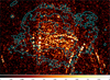 |
Fig. 4 Counts map (not vignetting-corrected) in 3-7 keV to show the effect of the stray light. The cyan contour corresponds to 0.5, 2, and 8 counts for W28 in 0.4-2 keV. |
Fitting results (Z=0.3 Z⊙) with 1σ error.
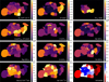 |
Fig. 5 Maps of the fitting parameters with a subsolar abundance Z=0.3Z⊙. The values of the parameters and their uncertainty correspond to Table 1. |
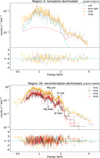 |
Fig. 6 Examples of spectra of underionized plasma (upper panel, region 3 in the western shell) and overionized plasma (lower panel, region 34 in the W28 center). In the upper panel, the contribution of the plasma and the stray light are marked with solid cyan lines and dashed red lines, respectively. The lower panel contains spectra of two observations, of which only the yellow and gray data points are significantly affected by the stray light. |
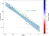 |
Fig. 7 Temperature-EM of the best-fit value of the EM and the temperature (circle dots). The solid blue line shows the best-fit power-law model, and the shadow shows the 90% confidence belt. The green diamonds and dashed lines mark the initial property of the recombining plasma on the assumption of an isobaric cooling. The color of the markers shows the ionization degrees, which are the same as in Fig. 5. |
4 Discussion
4.1 Temperature-EM diagram
The X-ray observations revealed varying plasma properties across SNR W28. A comparison of the density and temperature relation among regions can provide insight into the physical origin of this variation. For example, a random distribution might suggest no physical relations, while a power-law relation EM ∼ Tα can reflect the dynamical evolution of the plasma. A positive index α ≈ 3 (i.e., n ∼ T3/2) indicates adiabatic expansion, while a negative index α ≈ −2 (i.e., n ~ T−1 ) might indicate an isobaric scenario (Zhang et al. 2019). The power-law relation does not hold directly for the density and temperature themselves, but for their changes compared to the initial value. Here, a uniform temperature and density were assumed in the early stage of the SNR.
Figure 7 plots the relation between the best-fit values of EM (= nenHl) and kT (Fig. 7). We used EM instead of the density since it is a direct measurement that is proportional to the fitted parameter norm, but the density of the plasma is degenerate with the assumed geometry.
The EM-kT distribution can be divided into three different populations. In terms of the temperature, the coolest population is around ~0.1-0.2 keV and the gas is recombining. Most of these regions are distributed in the SNR interior. In contrast, the population with a temperature over 1 keV is underionized and is mostly located in the western shell and the southeastern lobe (region 46). The rest mainly has a temperature around 0.60.7 keV with various ionization degrees. However, the global distribution of these data points can be described by a power-law function, and the scatters generally fall within 1 dex.
The fitted power-law index α of  (90% statistical error) is probably indicative of the isobaric scenario where α = –2 (i.e., nT = const.). For the fitting result with the solar abundance, this isobaric correlation still exists with an index of —2.27 with relatively large scatter (see Appendix C). On a large scale, the plasma in W28 follows the near-isobaric relation. The western shell, originally identified as distinct SNRs, conforms to this relation and might therefore belong to W28.
For recombination dominated by thermal conduction, the gas is expected to experience an isobaric process. We mark the initial state of the recombining regions in Fig. 7 (green diamonds) assuming an isobaric heat exchange (i.e., α = -2). The distribution of the initial temperatures, derived from the fitted kTinit in Table 1, is mostly consistent with the 0.6-0.7 keV population, although the initial EMs are apparently higher within –0.5 dex. The 0.7-keV population dominant in the remnant center can be referred to as the initial state of the W28 gas before the cooling.
The absence of a strong pressure gradient rules out an efficient ongoing adiabatic cooling, even though the current isobaric conditions might have resulted from the relaxation of an earlier gradient. Simulations of thermal-composite SNRs revealed that the recombination due to adiabatic cooling is expected to take place near the shock interface and is not associated with cloudlets (see regions b and d, respectively, in Figs. 6 and 7 in Zhang et al. 2019). In W28, the recombining regions are strongly spatially coincident with Hα emission. This correspondence favors a thermal conduction origin over an adiabatic-cooling origin for the recombining plasma.
Compared to the temperature, the EM distribution shows a larger scatter, which can more or less account for the dependence of the density on the geometry. For SNRs, the radial distribution of the gas l can be roughly estimated under different scenarios. One scenario is that the X-ray-emitting gas is adiabatically swept into a thin shell with a depth of –1/12 of the remnant radius. The other extreme case corresponds to the hot gas uniformly filling the entire SNR. Therefore, the uncertainty of l is expected to lie within –1 dex, which leads to an uncertainty of the density only within about three times according to the definition of the EM. Moreover, the real spatial distribution of l is expected to be continuous in structures with a smooth surface brightness, such as the W28 center.
W28 has a radius of –20′ in the radio band, corresponding to ~11 pc at a distance of 1.9 kpc (Velázquez et al. 2002). Therefore, the radial depth l can be –1-22 parsecs. Considering the uncertainty of the geometry, the density is ~0.1-0.4, ~0.3-1.5, and –2-7 cm−3 for the western shell, the W28 center without recombination, and the recombining gas, respectively. This decreasing density gradient of W28 from east to west might account for the blow-out morphology of the western shell.
4.2 Origin of the recombining plasma
There has been no consensus on the origin of recombining plasma in SNRs, as it depends on the specific conditions of the SNR and the environment in which it evolves. Thermal conduction (Cox et al. 1999; Shelton et al. 1999; Zhou et al. 2014), cloud evaporation (Cowie et al. 1981; White & Long 1991; Long et al. 1991), adiabatic cooling (Itoh & Masai 1989; Zhang et al. 2019), or other mechanisms such as low-energy cosmic rays (Himono et al. 2023) are potential origins. With clumpy Hα emissions in the center, which show a different morphology from that of radiative shocks (Long et al. 1991; White & Long 1991), it is natural to consider that thermal conduction and cloud evaporation play an important role in the cooling.
From the spectral analysis, the recombination (or cooling) timescale can be roughly estimated as
 (3)
(3)
which is consistent with most areas in the W28 center according to a previous study Himono et al. (2023). This timescale indicates that the cooling took place recently compared to the dynamical timescale of ∼33-42kyr proposed before (Rho & Borkowski 2002; Velázquez et al. 2002; Li & Chen 2010) and ∼8 kyr suggested in our study (see the subsection below). It should be noted that trec might not be valid for the adiabatic cooling, where the density can drop rapidly.
Previous studies mainly focused on long-range classical thermal conduction (Zhou et al. 2014; Himono et al. 2023). The density gradient (Fig. 5) from east to west might support the scenario according to which the molecular clouds in the east are a cooling source. The long range means that the conduction scale exceeds the mean free path of the electron (Cowie & McKee 1977),
 (4)
(4)
The conduction timescale is
 (5)
(5)
where κ is the thermal conductivity as a function of temperature (see Eqs. (3)-(5) in Cowie & McKee 1977), and ln Λ = 32 + ln(ne/1cm−3)−1(kT/0.7keV) is the Coulomb logarithm. lT = T/∇T is the scale length of the temperature gradient, which can be considered as the size of the recombination region (Zhou et al. 2014; Himono et al. 2023). The long-range cooling timescale tcon is far longer than the recombination timescale of ∼3 kyr, and the magnetic field can suppress conduction. In other words, the long-range cooling might contribute, but only affects a small part of the SNR.
Therefore, we considered whether the small-scale saturated thermal conduction works efficiently in W28. One crucial indication is the clumpy Hα emissions in the remnant center (White & Long 1991; Long et al. 1991), which are found to be highly spatially correlated with the recombining regions in our analysis mentioned in the section above. One explanation of the Hα emission is that the gas evaporated from the cloud is heated to ∼104 K (White & Long 1991; Zhang et al. 2019). In numerical simulations, the temperature of most cloudlets can rapidly increase to ∼104 K behind the shock (Zhang et al. 2019) after it is engulfed by the shock. The clouds emitting Hα emission are likely in the interior of the SNR and not in the SNR shell, since they do not spatially coincide with any radio, infrared, or molecular structures.
We herein propose a toy model to briefly calculate the effect of saturated thermal conduction (Cowie & McKee 1977), where the heat flux is
 (6)
(6)
When the heat exchange occurs at the interface between the cloud and the hot gas, the heat transfer rate per unit volume to cool the hot gas is
 (7)
(7)
where rc is the average radius of the cloudlet, and Nc is the number density of cloudlets. By integrating this equation, we can obtain the evolution of Te under the saturated thermal conduction:
![Mathematical equation: \begin{split} t_\mathrm{sat} &=\frac{15}{8\pi r_\mathrm{c}^2N_\mathrm{c}}\left[\left(\frac{2kT_\mathrm{e}}{\pi m_\mathrm{e}}\right)^{-\frac{1}{2}}-\left(\frac{2kT_\mathrm{init}}{\pi m_\mathrm{e}}\right)^{-\frac{1}{2}}\right] \\ & =(5.7\,\mathrm{kyr})\,\left(\frac{r_\mathrm{c}}{0.1\,\mathrm{pc}}\right)^{-2}\left(\frac{N_\mathrm{c}}{1\,\mathrm{pc}^{-3}}\right)^{-1}, \end{split}](/articles/aa/full_html/2026/05/aa56500-25/aa56500-25-eq403.png) (8)
(8)
if kTe = 0.2 keV and kTinit = 0.7 keV. When we consider the mass loss of the cloudlets, the saturated thermal conduction timescale would be longer, but still comparable to the recombination timescale with a higher specific surface area (i.e., higher rc2 Nc). Therefore, the warm gas with a more diffuse distribution might play a more crucial role in the cooling than in denser cooler molecular clouds with a similar mass. In the Hα image, the scale size of the clumps is ∼10″, or ∼0.1 pc at 1.9kpc, which generally equals the mean free path of the electrons and is indicative of saturated thermal conduction.
The cloud evaporation takes place as the cold gas is heated by the saturated thermal conduction. The density, or rather, the EM in the recombining areas, is several times higher than those in CIE or underionization (see Fig. 7), suggesting that the X-ray-emitting gas therein is significantly enriched through the cloudlet evaporation. Under a rough estimation based on the EM measured in the spectral analysis, the evaporated gas might contribute ∼50-60 M⊙ mass.
Our X-ray spectral analysis (Sect. 3.2) revealed consistently subsolar metal abundances throughout W28 in the recombining regions dominated by evaporated cloud material and in the other regions with shocked low-density intercloud medium (ICM). This would be unusual given its location in the inner Galactic plane (G6.4–0.1), where near-solar metallicity is generally expected since the metallicity typically decreases with increasing galactocentric distance. However, it cannot be easily precluded as some H II regions and planet nebulae exhibit a [O/H] abundance 0.5-1 dex below this gradient (Maciel & Costa 2010; Wenger et al. 2019). The subsolar abundance of neon, an element largely inert to dust depletion, argues against dust depletion being the primary cause. We cannot rule out the possibility either that an additional continuum component affects the abundance measurements. Thus, the apparently low metal abundance in W28, a feature also noted in other SNRs such as the Cygnus Loop (e.g., Katsuda et al. 2008), remains an open question, likely requiring future multiwavelength analysis and X-ray missions with high spectral resolution.
We briefly compare the toy model here with the selfsimilarity model to describe the cloud evaporation (White & Long 1991) to end this subsection. In their study, the dimensionless parameter C is the mass ratio of the cloudlets and ICM, and τ̄ (using a bar marker to distinguish it from the ionization timescale) is the ratio of the timescale on which the cloud depletes through evaporation (evaporation timescale tevap) to the age, or the dynamical timescale tdyn here, of the SNR. According to its definition, we can derive
 (9)
(9)
where nc is the density in the cloudlet, and n0 is the pre-shock ICM density. Long et al. (1991) derived a density of ∼25 cm−3 from the [S II] doublet ratio, which corresponds to a temperature of ∼104 K, and the cloudlet would be even denser with a lower temperature. Along with the shocked gas density of ∼ 1 cm−3 without recombination in the W28 center, we estimate that the lower limit of nc/n0 is around 100. On the other hand, Eq. (7) can be rewritten to describe the mass loss as
 (10)
(10)
Thus, the evaporation timescale can be described as the ratio of the cloudlet size rc to its rate,
 (11)
(11)
where ne = 4.8n0 assuming the electron density corresponds to the shocked ICM with fully ionized H and He. A larger τ̄ = tevap/tdyn ≳ 1 is favored for the cloudlet evaporation (White & Long 1991), which might suggest a shorter dynamical timescale of ∼8 kyr (see the subsection below) instead of ∼33-42 kyr proposed in previous studies (Rho & Borkowski 2002; Velázquez et al. 2002; Li & Chen 2010), although the cloudlet density is highly uncertain. We obtained the relation between C and τ̄ under the saturated conduction, which is independent of the density ratio,
 (12)
(12)
In the model of White & Long (1991), 1 ≲ τ̄ ≲ C is needed to allow the cloudlet evaporation to be efficient and show a morphology deviating from that predicted by the Sedov-Taylor solution.
4.3 The western shell and its physical connection to W28
The most evident newly discovered structure revealed by the large field of view of our EP-FXT observations is the shell-like structure west of W28. Currently, these observations support its shock origin, including
a shell-like morphology in radio, optical, and X-ray bands (Sect. 3.1);
an underionized hot plasma (Sect. 3.2), enhanced [S II]/Hα, and a nonthermal radio index (see references in Sect. 3.1).
Although further observations are needed to definitely establish the relation between this structure and W28, some evidence supports the hypothesis that the western shell is part of the SNR W28:
All of these shells, including the newly discovered western shell and the previously known southwestern shell (clumps D and E), share similar rather than random orientations. It is therefore reasonable to assume that these shells originated from an explosion near the W28 center (Fig. 3).
These shells share a similar foreground absorption with the W28 center (Sect. 3.2).
The shells and the W28 center are generally isobaric (Sect.4.1).
If the western shell belongs to W28, its dynamical age matches that of clump E to the southwest (see details below). Using the parameters of the shell-like structures, we roughly estimated the dynamical age and explosion energy with the Sedov-Taylor solution. For a nonrelativistic strong shock, its velocity depends on its temperature,
 (13)
(13)
where the electron and ion are assumed to share the same temperature and the mean particle mass μ = 0.6 for solar abundance, and mp is the proton mass. Evolving isotropically and adiabatically in a uniform medium, the dynamical age can be given by
 (14)
(14)
where D1.9 is the distance of W28 in units of 1.9 kpc (Velázquez et al. 2002), and θ is the radius of the shell from the center.
For regions 1-3, the temperature is ∼1.5 keV, and the angular distance from the remnant center is ∼40′, corresponding to tdyn = 7.6 kyr. Coincidentally, tdyn = 7.8 kyr for region 10 (clump E) at the southwestern boundary of the radio shell, which is ∼30′ away from the center and has a fitting temperature of ∼0.8 keV. This dynamical timescale is generally consistent with the ionization timescale of ∼1010 s cm−3 in the western shell (assuming ne ∼ 0.2 cm−3) and ∼1011 s cm−3 in the southwest (assuming ne ∼ 1 cm−3). This dynamical timescale is reasonably longer than the recombination timescale trec ∼ 3 kyr. However, it is much shorter than several tens of kilo-years in previous studies (Rho & Borkowski 2002; Velázquez et al. 2002; Li & Chen 2010), which were based on the velocity of optical emissions (e.g., Hα) and an assumption of radiative phase. The expansion velocity of ∼80 km s−1 derived from the optical emission reflects the low shock velocity in the dense medium.
For an SNR evolving in a Sedov-Taylor phase, the explosion energy can also be estimated through
 (15)
(15)
where the dimensionless factor ξ = 2.025, the ambient density ρ0 = 1.4mpn/4. Thus, we can roughly estimate the explosion energy of W28 of ∼(1-2) × 1051 erg according to the western and the southwestern shell. If evolving in a wind bubble, the dynamical age and explosion energy would be ∼1.5 times of the values above (see Chi et al. 2024, and references therein). It should be noted that these calculations are based on the assumption that these structures are part of the SNR. If these shells are separate SNRs at different distances, their radius and evolutionary stage could largely deviate from the above results.
W28 is one of the prototypical thermal-composite SNRs (Long et al. 1991), and its morphology deviates from the prediction of the Sedov-Taylor model, but later studies reported that its morphology cannot be perfectly explained by any available physical models for thermal-composite SNRs (Rho & Borkowski 2002). We suggest that the shell-like and thermal-composite morphology can coexist in one SNR due to different environments in different directions. In the first 4-5kyr, W28 might have evolved as a typical shell-like SNR until it reached a large size of some tens of parsecs. After this, it is reasonable that different parts of a medium-age SNR evolve in different environments. Once in a dense medium, the cloud evaporation and thermal conduction might be significant, leading to centrally brightened X-ray emissions with recombination features, while in other directions with lower density, a continuous evolution in the Sedov-Taylor phase formed the western shell of W28.
5 Conclusion
We showed EP-FXT studies of the prototypical thermalcomposite SNR W28. The large field of view of FXT maps this large SNR with a high efficiency and provides new insights into this remnant. We report them below:
We discovered a new X-ray shell-like emission feature west of the W28 center and spatially associated with its counterparts in radio and optical wavelengths. It shares a similar pressure and foreground absorption with the gas in the W28 center, but has a high electron temperature of ∼1.5 keV and is underionized. These properties, together with the shell orientation, suggest that they are part of SNR W28. Adopting this assumption, we estimated a dynamical age of ∼8 kyr, which is much younger than in previous studies, and an explosion energy of ∼(1-2) × 1051 erg;
The EP-FXT observation revealed a complex morphology of W28 and its vicinity, with a western shell and several clumps in addition to its thermal-composite center. The spectral analysis presented the spatial distribution of the ionization status of the hot plasma in W28. The recombining plasma with a low electron temperature of ∼0.2 keV and initial temperature of ∼0.6-0.7 keV is spatially coincident with Hα emission in the W28 center. The other regions show plasma in ionizing or CIE states, and the western shell has a high temperature of > 1 keV. Generally, the heavy element abundances of the hot gas are subsolar;
We found a similarity between the initial temperature tinit of the recombining plasma and the current temperature T of the CIE plasma and a nearly smooth distribution of max(tinit, T) in most regions of W28. This suggests that most areas of W28 were generally isothermal with a temperature of ~0.7 keV before the plasma cooling;
We used a kT-EM diagram of the regions and found a near isobaric distribution. This suggests that the western shell and the W28 center might share a physical origin and that the recombination in W28 is probably dominated by thermal conduction instead of adiabatic expansion. We estimated a recombination timescale of ∼3 kyr, which is more likely to arise from the short-range saturated thermal conduction and cloud evaporation than from long-range conduction;
The complex morphology and ionization state distribution of W28 are probably the result of its evolution in an environment with a high density gradient. The shell-like and thermal-composite morphology could coexist in one SNR, as the morphology originates more from nurture than nature.
Acknowledgements
We would like to express our sincere gratitude to the referee for their constructive comments, which have greatly improved the paper. We thank Fangjun Lu for helpful discussions in SNR science with EP and for requesting the W28 observations. This work is based on the data obtained with Einstein Probe, a space mission supported by the Strategic Priority Program on Space Science of Chinese Academy of Sciences, in collaboration with the European Space Agency, the Max-Planck-Institute for extraterrestrial Physics (Germany), and the Centre National d’Études Spatiales (France). This study is based on observations obtained with XMM-Newton, an ESA science mission with instruments and contributions directly funded by ESA Member States and NASA. This research made use of the data from the Milky Way Imaging Scroll Painting (MWISP) project, which is a multi-line survey in 12CO/13CO/C18O along the northern galactic plane with PMO-13.7m telescope. We are grateful to all the members of the MWISP working group, particularly the staff members at PMO-13.7m telescope, for their long-term support. Y.-H.C. acknowledges supports from the National Natural Science Foundation of China (NSFC) via grant NSFC 123B1021. P.Z. thanks the support by NSFC 12273010, the Fundamental Research Funds for the Central Universities No. KG202502, the China Manned Space Program with grant nos. CMS-CSST-2025-A14 and CMS-CSST-2025-A18. Y.C. acknowledges NSFC under grants 12121003 and 12573047. L.S. thanks the support from NSFC grant No. 12503030. C.G. acknowledges the foundation from the grant NFSC 12373007 and 12422302. MWISP was sponsored by National Key R&D Program of China with grant 2017YFA0402701 and CAS Key Research Program of Frontier Sciences with grant QYZDJ-SSW-SLH047.
References
- Abdo, A. A., Ackermann, M., Ajello, M., et al. 2010, ApJ, 718, 348 [Google Scholar]
- Aharonian, F., Akhperjanian, A. G., Bazer-Bachi, A. R., et al. 2008, A&A, 481, 401 [NASA ADS] [CrossRef] [EDP Sciences] [Google Scholar]
- Arikawa, Y., Tatematsu, K., Sekimoto, Y., & Takahashi, T. 1999, PASJ, 51, L7 [Google Scholar]
- Arnaud, K. A. 1996, in Astronomical Society of the Pacific Conference Series, 101, Astronomical Data Analysis Software and Systems V, eds. G. H. Jacoby, & J. Barnes, 17 [Google Scholar]
- Blackburn, J. K. 1995, in Astronomical Society of the Pacific Conference Series, 77, Astronomical Data Analysis Software and Systems IV, eds. R. A. Shaw, H. E. Payne, & J. J. E. Hayes, 367 [Google Scholar]
- Brogan, C. L., Gelfand, J. D., Gaensler, B. M., Kassim, N. E., & Lazio, T. J. W. 2006, ApJ, 639, L25 [Google Scholar]
- Chen, Y., Seward, F. D., Sun, M., & Li, J.-t. 2008, ApJ, 676, 1040 [NASA ADS] [CrossRef] [Google Scholar]
- Chen, Y., Cui, W., Han, D., et al. 2020, SPIE Conf. Ser., 11444, 114445B [Google Scholar]
- Chen, Y., Wang, J., Yang, Y., et al. 2025, Radiat. Detect. Technol. Methods, 9, 198 [Google Scholar]
- Chevalier, R. A. 1982, ApJ, 258, 790 [NASA ADS] [CrossRef] [Google Scholar]
- Chi, Y.-H., Huang, J., Zhou, P., et al. 2024, ApJ, 975, L28 [Google Scholar]
- Claussen, M. J., Frail, D. A., Goss, W. M., & Gaume, R. A. 1997, ApJ, 489, 143 [NASA ADS] [CrossRef] [Google Scholar]
- Cowie, L. L., & McKee, C. F. 1977, ApJ, 211, 135 [NASA ADS] [CrossRef] [Google Scholar]
- Cowie, L. L., McKee, C. F., & Ostriker, J. P. 1981, ApJ, 247, 908 [NASA ADS] [CrossRef] [Google Scholar]
- Cox, D. P., Shelton, R. L., Maciejewski, W., et al. 1999, ApJ, 524, 179 [NASA ADS] [CrossRef] [Google Scholar]
- Cui, Y., Yeung, P. K. H., Tam, P. H. T., & Pühlhofer, G. 2018, ApJ, 860, 69 [Google Scholar]
- Ferrand, G., & Safi-Harb, S. 2012, Adv. Space Res., 49, 1313 [Google Scholar]
- Foster, A. R., Ji, L., Smith, R. K., & Brickhouse, N. S. 2012, ApJ, 756, 128 [Google Scholar]
- Frail, D. A., Goss, W. M., & Slysh, V. I. 1994, ApJ, 424, L111 [Google Scholar]
- Fruscione, A., McDowell, J. C., Allen, G. E., et al. 2006, SPIE Conf. Ser., 6270, 62701V [Google Scholar]
- Gabriel, C., Denby, M., Fyfe, D. J., et al. 2004, in Astronomical Society of the Pacific Conference Series, 314, Astronomical Data Analysis Software and Systems (ADASS) XIII, ed. F. Ochsenbein, M. G. Allen, & D. Egret, 759 [Google Scholar]
- Goedhart, S., Cotton, W. D., Camilo, F., et al. 2024, MNRAS, 531, 649 [CrossRef] [Google Scholar]
- Hands, A. D. P., Warwick, R. S., Watson, M. G., & Helfand, D. J. 2004, MNRAS, 351, 31 [Google Scholar]
- Himono, R., Nobukawa, M., Yamauchi, S., Nobukawa, K. K., & Suzuki, N. 2023, PASJ, 75, 373 [Google Scholar]
- Hoffman, I. M., Goss, W. M., Brogan, C. L., & Claussen, M. J. 2005, ApJ, 620, 257 [Google Scholar]
- Itoh, H., & Masai, K. 1989, MNRAS, 236, 885 [Google Scholar]
- Jansen, F., Lumb, D., Altieri, B., et al. 2001, A&A, 365, L1 [NASA ADS] [CrossRef] [EDP Sciences] [Google Scholar]
- Katsuda, S., Tsunemi, H., Kimura, M., & Mori, K. 2008, ApJ, 680, 1198 [NASA ADS] [CrossRef] [Google Scholar]
- Kawasaki, M., Ozaki, M., Nagase, F., Inoue, H., & Petre, R. 2005, ApJ, 631, 935 [Google Scholar]
- Lazendic, J. S., & Slane, P. O. 2006, ApJ, 647, 350 [Google Scholar]
- Li, H., & Chen, Y. 2010, MNRAS, 409, L35 [NASA ADS] [CrossRef] [Google Scholar]
- Long, K. S., Blair, W. P., White, R. L., & Matsui, Y. 1991, ApJ, 373, 567 [Google Scholar]
- Maciel, W. J., & Costa, R. D. D. 2010, in IAU Symposium, 265, Chemical Abundances in the Universe: Connecting First Stars to Planets, eds. K. Cunha, M. Spite, & B. Barbuy, 317 [Google Scholar]
- Mavromatakis, F., Aschenbach, B., Boumis, P., & Papamastorakis, J. 2004, A&A, 415, 1051 [NASA ADS] [CrossRef] [EDP Sciences] [Google Scholar]
- Mazumdar, P., Tram, L. N., Wyrowski, F., Menten, K. M., & Tang, X. 2022, A&A, 668, A180 [NASA ADS] [CrossRef] [EDP Sciences] [Google Scholar]
- Mitsuda, K., Bautz, M., Inoue, H., et al. 2007, PASJ, 59, S1 [NASA ADS] [CrossRef] [Google Scholar]
- Nakamura, R., Bamba, A., Ishida, M., et al. 2014, PASJ, 66, 62 [Google Scholar]
- Okon, H., Uchida, H., Tanaka, T., Matsumura, H., & Tsuru, T. G. 2018, PASJ, 70, 35 [NASA ADS] [CrossRef] [Google Scholar]
- Ono, A., Uchiyama, H., Yamauchi, S., et al. 2019, PASJ, 71, 52 [Google Scholar]
- Pannuti, T. G., Rho, J., Kargaltsev, O., et al. 2017, ApJ, 839, 59 [Google Scholar]
- Parker, Q. A., Phillipps, S., Pierce, M. J., et al. 2005, MNRAS, 362, 689 [NASA ADS] [CrossRef] [Google Scholar]
- Reach, W. T., Rho, J., & Jarrett, T. H. 2005, ApJ, 618, 297 [NASA ADS] [CrossRef] [Google Scholar]
- Rho, J., & Petre, R. 1998, ApJ, 503, L167 [NASA ADS] [CrossRef] [Google Scholar]
- Rho, J., & Borkowski, K. J. 2002, ApJ, 575, 201 [NASA ADS] [CrossRef] [Google Scholar]
- Rowell, G. P., Naito, T., Dazeley, S. A., et al. 2000, A&A, 359, 337 [NASA ADS] [Google Scholar]
- Sawada, M., & Koyama, K. 2012, PASJ, 64, 81 [Google Scholar]
- Sedov, L. I. 1959, Similarity and Dimensional Methods in Mechanics (New York: Academic Press) [Google Scholar]
- Sezer, A., Ergin, T., Yamazaki, R., Sano, H., & Fukui, Y. 2019, MNRAS, 489, 4300 [NASA ADS] [CrossRef] [Google Scholar]
- Shelton, R. L., Cox, D. P., Maciejewski, W., et al. 1999, ApJ, 524, 192 [NASA ADS] [CrossRef] [Google Scholar]
- Shelton, R. L., Kuntz, K. D., & Petre, R. 2004, ApJ, 615, 275 [Google Scholar]
- Shimizu, T., Masai, K., & Koyama, K. 2012, PASJ, 64, 24 [NASA ADS] [Google Scholar]
- Strüder, L., Briel, U., Dennerl, K., et al. 2001, A&A, 365, L18 [Google Scholar]
- Stupar, M., & Parker, Q. A. 2011, MNRAS, 414, 2282 [Google Scholar]
- Stupar, M., Parker, Q. A., & Frew, D. J. 2018, MNRAS, 479, 4432 [Google Scholar]
- Taylor, G. 1950, Proc. Roy. Soc. London Ser. A, 201, 159 [NASA ADS] [CrossRef] [Google Scholar]
- Tu, T-Y., Chen, Y., Zhou, P., Safi-Harb, S., & Liu, Q.-C. 2024, ApJ, 966, 178 [NASA ADS] [CrossRef] [Google Scholar]
- Turner, M. J. L., Abbey, A., Arnaud, M., et al. 2001, A&A, 365, L27 [CrossRef] [EDP Sciences] [Google Scholar]
- Velázquez, P. F., Dubner, G. M., Goss, W. M., & Green, A. J. 2002, AJ, 124, 2145 [CrossRef] [Google Scholar]
- Weisskopf, M. C., Brinkman, B., Canizares, C., et al. 2002, PASP, 114, 1 [NASA ADS] [CrossRef] [Google Scholar]
- Wenger, M., Ochsenbein, F., Egret, D., et al. 2000, A&AS, 143, 9 [NASA ADS] [CrossRef] [EDP Sciences] [Google Scholar]
- Wenger, T. V., Balser, D. S., Anderson, L. D., & Bania, T. M. 2019, ApJ, 887, 114 [NASA ADS] [CrossRef] [Google Scholar]
- White, R. L., & Long, K. S. 1991, ApJ, 373, 543 [NASA ADS] [CrossRef] [Google Scholar]
- Wilms, J., Allen, A., & McCray, R. 2000, ApJ, 542, 914 [Google Scholar]
- Yamaguchi, H., Ozawa, M., Koyama, K., et al. 2009, ApJ, 705, L6 [NASA ADS] [CrossRef] [Google Scholar]
- Yuan, W., Zhang, C., Chen, Y., & Ling, Z. 2022, in Handbook of X-ray and Gamma-ray Astrophysics, eds. C. Bambi, & A. Sangangelo (Singapore: Springer Nature Singapore), 86 [Google Scholar]
- Zhang, G.-Y., Slavin, J. D., Foster, A., et al. 2019, ApJ, 875, 81 [Google Scholar]
- Zhang, J., Qi, L., Yang, Y., et al. 2022, Astropart. Phys., 137, 102668 [Google Scholar]
- Zhou, P., Safi-Harb, S., Chen, Y., et al. 2014, ApJ, 791, 87 [Google Scholar]
Appendix A Details of the X-ray observations
The details of the EP-FXT and XMM-Newton observations are listed in Table A.1.
EP-FXT and XMM-Newton observations.
Appendix B FXT versus XMM-Newton: Calibration and limitation
The EP-FXT PV phase observations were performed before the completion of the first in-orbit calibration. Although the raw data have been updated with the latest calibration database, it is still necessary to use reliable and well-calibrated data from other X-ray telescopes for cross-calibration. With high surface brightness, the NE shell (Region 44, in Fig. 3) is an appropriate source for calibration in our field of view. Besides, located in the upper part of the detector, or rather further from GX 5–1, this region appears to suffer from minimal contamination of the stray light.
We first used a CIE model (vapec) to fit the FXT spectra in 0.5-2.0keV with good statistic quality and minimal influence from the stray light. The best-fit model (χ2r/dof=1.35/233, where dof is short for degrees of freedom) gives an absorption of NH=7.3 × 1021 cm−2, a temperature of 0.47 keV, and subsolar Ne, Mg, Si, and Fe. However, a residual appears near 0.9 keV, which is more evident if all the XMM-Newton and FXT spectra are fitted jointly. Therefore, the CIE model is substituted by an overionized NEI model (vrnei), effectively improving the fitting statistics to χ2r/dof=1.15/232 (see Table B.1 and Fig. B.1). The abundance of O, Ne, Mg, and Si seems subsolar while the Fe abundance cannot be constrained well and thus fixed to solar abundance as other metals. The ionization timescale is around 1012 s cm−3, quite close to CIE and probably leading to a poor constraint of the initial temperature.
Then, a similar model was used to fit the XMM-Newton spectra (see Table B.1 and Fig. B.2). For each spectrum, a constant component is multiplied to reflect its relative intensity, which can be affected by the calibration uncertainties, CCD gaps, or bad pixels in the region. Generally, due to the longer exposure and large effective area, the XMM-Newton data can better constrain the parameters. The major difference in the fitting results is that XMM-Newton gives a slightly higher absorption and metal abundance, while the temperature, ionization timescale, and emission measure are consistent within the 1σ uncertainty.
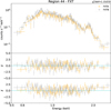 |
Fig. B.1 Upper panel: FXTA (marked in orange) and FXTB (marked in grey) spectra of the NE shell (Region 44). Middle panel: Residuals of the best-fit model. Lower panel: Residuals to compare the FXT spectra with the XMM-Newton model after rescaling the normalizations. |
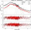 |
Fig. B.2 Upper panel: XMM-Newton pn (marked in black) and MOS (marked in red) spectra of the NE shell (Region 44). Dashed lines show the model folded with the response file. Different levels of transparency stand for different observations and different cameras (i.e., MOS 1 and 2). The components of one MOS spectra were displayed as well, including the astrophysical background (the yellow dashed line), instrument fluorescence lines (Al and Si, the grey dash-dot line), overionized plasma (the cyan solid line), and extra Gaussian components for emission lines (dotted lines in different colors). Middle panel: Residuals of the best-fit model without extra line components. Lower panel: Residuals of the best-fit panel. |
Fitting results of regions 44 and 26 for calibration with 1σ uncertainties.
The fitted parameters obtained through the XMM-Newton data were then compared to the FXT spectra. The average intensity of FXT and XMM-Newton data is consistent within 10%. We found that the XMM-Newton model fit the FXT spectra best in the 0.8-2.0 keV band, which covers the line emissions of Fe, Ne, Mg, and Si. However, in lower and higher energy bands with low count rates, FXT data points seem to be higher than the XMM-Newton model.
Noticeably, one single vrnei model cannot explain the entire XMM-Newton spectra. Evident residuals are present near 0.5, 2.4, 2.6, 3.1, and 6.7 keV (Fig. B.2), probably corresponding to the N VII, S XV, S XVI, Ar XVII, and Fe K lines or related RRC, respectively. For instance, the likely S and Ar line features are expected to originate from an extra higher-temperature component to explain the excess above 2 keV in the FXT spectra, precluding very high non-thermal emissions scenario. Therefore, we added 5 extra gaussian components to the vrnei model to improve the fitting.
We also compared the spectra between two missions of Region 26, where the X-ray surface brightness peaks in the W28 center. With a lower exposure and far from the optical axis of XMM-Newton, we simply listed the fitting results in Table B.1. The results are similar to those of Region 44. FXT gives a lower column density than XMM-Newton, which may correspond to higher FXT data points of FXT below ~ 0.8 keV as mentioned before and plotted in Fig. B.1. The abundances of heavy elements are generally subsolar in spite of some differences in some specific metals like Ne. The electron temperature, emission measure, and ionization timescale are generally consistent within ~ 1σ uncertainties.
Appendix C Fitting results with solar abundance
Here we show the fitting parameters with solar abundance as the default, including Table C.1, the temperature-EM map (Fig. C.1), and the parameter map (Fig. C.2).
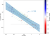 |
Fig. C.1 Same as Fig. 7 but the data points are based on the spectral analysis with default solar abundances. The uncertainty of index and the confidence belt correspond to 1σ confidence level due to a larger data dispersion here. |
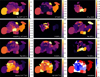 |
Fig. C.2 Maps of fitting result (Z=Z⊙). Fixed parameters are set to blank here. |
Fitting results (Z=Z⊙) with 1σ error.
The vrnei model describes the recombination of the plasma in CIE initially. However, the real picture might be that the plasma is first shocked and heated, and then, before it reaches CIE, the recombination begins. This scenario is so complex that it exceeds the range of our study, and most regions have an ionization timescale of ∼1012 cm−3 s, close to CIE.
All Tables
All Figures
|
Fig. 1 Energy-coded X-ray image of the W28 complex with FXT (a), consisting of bands in 0.4-0.7 keV (red), 0.7-1.1 keV (green), and 1.12.3 keV (blue). The single-band images of each energy band are shown in panels (b), (c), and (d). The images are in units of count s−1 cm−2 and in a square-root color scale to enhance weak emissions. All the images are vignetting-corrected and adaptively smoothed. The structures mentioned in this paper are marked in panels (c) and (d). The cyan regions correspond to optical and/or radio SNR candidates (Stupar & Parker 2011; Stupar et al. 2018). |
| In the text | |
|
Fig. 2 (a) Same as Fig. 1a but based on XMM-Newton data. The arc-like patterns of the stray light from GX 5-1 are visible in the south, marked between dashed white lines. (b) Effective exposure time of XMM-Newton in units of ks scaled as MOS2 with the Medium filter, which shares a similar effective area with one FXT module. |
| In the text | |
|
Fig. 3 Tricolor image of W28 in the radio (red, 1.3 GHz continuum), Hα (green), and X-ray (blue, 0.4-2.3 keV) bands. A square root color scale is used to highlight faint diffuse emissions in the radio and X-ray images. The white polygon regions are used for spectral extraction and analysis, and the dashed cyan regions correspond to the sky background. The yellow contours correspond to the MWISP CO intensity in the –20-10 km s−1 (Tu et al. 2024). The optical nebulae southeast and northeast of W28 are the Lagoon Nebula Messier 8 and the Trifid Nebula Messier 20, respectively. |
| In the text | |
|
Fig. 4 Counts map (not vignetting-corrected) in 3-7 keV to show the effect of the stray light. The cyan contour corresponds to 0.5, 2, and 8 counts for W28 in 0.4-2 keV. |
| In the text | |
|
Fig. 5 Maps of the fitting parameters with a subsolar abundance Z=0.3Z⊙. The values of the parameters and their uncertainty correspond to Table 1. |
| In the text | |
|
Fig. 6 Examples of spectra of underionized plasma (upper panel, region 3 in the western shell) and overionized plasma (lower panel, region 34 in the W28 center). In the upper panel, the contribution of the plasma and the stray light are marked with solid cyan lines and dashed red lines, respectively. The lower panel contains spectra of two observations, of which only the yellow and gray data points are significantly affected by the stray light. |
| In the text | |
|
Fig. 7 Temperature-EM of the best-fit value of the EM and the temperature (circle dots). The solid blue line shows the best-fit power-law model, and the shadow shows the 90% confidence belt. The green diamonds and dashed lines mark the initial property of the recombining plasma on the assumption of an isobaric cooling. The color of the markers shows the ionization degrees, which are the same as in Fig. 5. |
| In the text | |
|
Fig. B.1 Upper panel: FXTA (marked in orange) and FXTB (marked in grey) spectra of the NE shell (Region 44). Middle panel: Residuals of the best-fit model. Lower panel: Residuals to compare the FXT spectra with the XMM-Newton model after rescaling the normalizations. |
| In the text | |
|
Fig. B.2 Upper panel: XMM-Newton pn (marked in black) and MOS (marked in red) spectra of the NE shell (Region 44). Dashed lines show the model folded with the response file. Different levels of transparency stand for different observations and different cameras (i.e., MOS 1 and 2). The components of one MOS spectra were displayed as well, including the astrophysical background (the yellow dashed line), instrument fluorescence lines (Al and Si, the grey dash-dot line), overionized plasma (the cyan solid line), and extra Gaussian components for emission lines (dotted lines in different colors). Middle panel: Residuals of the best-fit model without extra line components. Lower panel: Residuals of the best-fit panel. |
| In the text | |
|
Fig. C.1 Same as Fig. 7 but the data points are based on the spectral analysis with default solar abundances. The uncertainty of index and the confidence belt correspond to 1σ confidence level due to a larger data dispersion here. |
| In the text | |
|
Fig. C.2 Maps of fitting result (Z=Z⊙). Fixed parameters are set to blank here. |
| In the text | |
Current usage metrics show cumulative count of Article Views (full-text article views including HTML views, PDF and ePub downloads, according to the available data) and Abstracts Views on Vision4Press platform.
Data correspond to usage on the plateform after 2015. The current usage metrics is available 48-96 hours after online publication and is updated daily on week days.
Initial download of the metrics may take a while.