| Issue |
A&A
Volume 700, August 2025
|
|
|---|---|---|
| Article Number | A6 | |
| Number of page(s) | 13 | |
| Section | The Sun and the Heliosphere | |
| DOI | https://doi.org/10.1051/0004-6361/202554524 | |
| Published online | 25 July 2025 | |
Improving the Γ-functions method for vortex identification
1
National Key Laboratory of Deep Space Exploration, School of Earth and Space Sciences, University of Science and Technology of China, Hefei 230026, China
2
CAS Center for Excellence in Comparative Planetology/CAS Key Laboratory of Geospace Environment/Mengcheng National Geophysical Observatory, University of Science and Technology of China, Hefei 230026, China
3
Solar Physics and Space Plasma Research Centre (SP2RC), School of Mathematical and Physical Sciences, University of Sheffield, Sheffield S3 7RH, UK
4
Department of Astronomy, Eötvös Loránd University, Budapest, Pázmány P. sétány 1/A H-1117, Hungary
5
Gyula Bay Zoltan Solar Observatory (GSO), Hungarian Solar Physics Foundation (HSPF), Petőfi tér 3., Gyula H-5700, Hungary
⋆ Corresponding author: jiajialiu@ustc.edu.cn
Received:
14
March
2025
Accepted:
20
May
2025
Context. Vortices have been observed at various heights within the solar atmosphere and are suggested to play a significant role in heating the solar upper atmosphere. Multiple automated vortex detection methods have been developed and applied to identify vortices.
Aims. We aim to improve the Γ-functions method for vortex identification by optimizing the value of Γ1min and the approach to calculate Γ1 and Γ2, used to determine the center and edge of the vortex. This optimization enhances detection accuracy and enables statistical studies to improve our understanding of vortex generation and evolution in the solar atmosphere.
Methods. We applied the automated swirl detection algorithm (ASDA, a representative of the Γ-functions method) with different parameters to various synthetic datasets, each containing 1000 Lamb-Oseen vortices, to identify the optimal Γ1min and kernel size when calculating Γ1 and Γ2. We also compared another detection method using simulation and observational data to validate the results obtained from the synthetic datasets.
Results. We achieve the best performance with the Optimized ASDA, which combines different kernel sizes (5, 7, 9, and 11) to calculate Γ1 and Γ2 with Γ1min fixed at 0.63 for vortex center detection. We find that more vortices can be detected by the optimized ASDA with improved accuracy in location, radius, and rotation speed. These results are further confirmed by comparing vortices detected by the Optimized ASDA and the SWirl Identification by Rotation-centers Localization (SWIRL) method on CO5BOLD numerical simulation data and Swedish 1-m Solar Telescope observational data.
Key words: Sun: chromosphere / Sun: photosphere
© The Authors 2025
 Open Access article, published by EDP Sciences, under the terms of the Creative Commons Attribution License (https://creativecommons.org/licenses/by/4.0), which permits unrestricted use, distribution, and reproduction in any medium, provided the original work is properly cited.
This article is published in open access under the Subscribe to Open model. Subscribe to A&A to support open access publication.
1. Introduction
Rotational motions, spanning a wide range of spatial scales, have been widely observed at various heights in the solar atmosphere (e.g., Wang et al. 1995, 2016; Li et al. 2012; Liu et al. 2012; Su et al. 2012; Wedemeyer-Böhm et al. 2012; Panesar et al. 2013; Liu et al. 2019b,c; Tziotziou et al. 2023). Numerous studies have highlighted their potentially significant role in channeling energy to the upper solar atmosphere. It is widely accepted that various modes of magnetohydrodynamic (MHD) waves, particularly Alfvén waves and pulses, are associated with various vortices, as demonstrated by numerical simulations (e.g., Shelyag et al. 2013; Chmielewski et al. 2014; Mumford et al. 2015; Mumford & Erdélyi 2015; Liu et al. 2019c; Battaglia et al. 2021; Kesri et al. 2024). Observational evidence also supports this connection. For example, Wedemeyer-Böhm et al. (2012) reported that magnetic tornadoes act as energy channels into the solar corona, based on the manual detection of chromospheric vortices. Additionally, Liu et al. (2019c) used an automated algorithm to detect small-scale vortices, providing evidence that ubiquitous Alfvén pulses, triggered by photospheric vortices, transport energy to the upper chromosphere. Tziotziou et al. (2019) performed spectral analysis of a 1.7-hour vortex flow characterized by multiple intermittent chromospheric swirls and found dominant oscillations around four minutes, with both swaying (200–220 s) and rotational motions, as well as significant oscillatory power up to ten minutes, indicating the presence of various MHD wave modes at different heights. Tziotziou et al. (2020) further provide observational evidence of fast kinks and localized torsional waves associated with small chromospheric swirls and swaying motions within a persistent vortex flow. Small-scale vortices in the photosphere are also believed to contribute to energizing the upper atmosphere (e.g., Parker 1983; Velli & Liewer 1999; Shelyag et al. 2013). Furthermore, theoretical studies suggest that rotational motions can generate upward mass and momentum transfer, thereby leading to the generation of small-scale jets (spicules, e.g., Scalisi et al. 2021, 2023).
Over time, vortex motions in the solar atmosphere have been classified into several types based on their dynamic characteristics and formation mechanisms. The term “tornado” in the solar context was first introduced by Pettit (1932) to describe vortex motions, particularly those associated with prominences. This category includes solar tornadoes (Pike & Mason 1998), giant tornadoes (Li et al. 2012; Su et al. 2012), magnetic tornadoes (Wedemeyer-Böhm et al. 2012), and small-scale tornadoes (Tziotziou et al. 2018). Smaller vortical phenomena have been called “swirls”, which include chromospheric swirls (Wedemeyer-Böhm & van der Voort 2009), small-scale swirls (Shetye et al. 2019), magnetic swirls (e.g., Chmielewski et al. 2014; Murawski et al. 2018), and downdraft swirls (Moll et al. 2011). Additionally, the term “vortex” is often used in theoretical contexts derived from simulations, such as vortex tubes (Muthsam et al. 2010), horizontal vortex tubes (Steiner et al. 2010), magnetized vortex tubes (Kitiashvili et al. 2013), and kinetic (K-) and magnetic (M-) vortices (e.g., Silva et al. 2020, 2021). One notable exception is the “photospheric intensity vortex,” which, unlike the others, originates from observational data and is often called “swirls” (e.g., Giagkiozis et al. 2018; Liu et al. 2019b,c). In this work, we focus on the automated detection of small-scale vortices (also referred to as “swirls”).
Accurately and efficiently detecting small-scale vortices from observations has long been a key challenge. The first step in identifying numerous small-scale vortices from observational images is to reconstruct the horizontal velocity field for each image. Techniques such as local correlation tracking (LCT; November & Simon 1988), Fourier local correlation tracking (FLCT; Fisher & Welsch 2008), and coherent structure tracking (CST; Rieutord et al. 2007) use two consecutive intensity images to estimate the velocity field at the photosphere. DeepVel (Ramos et al. 2017) and its U-Net version, DeepVelU (Tremblay & Attie 2020), are deep, fully convolutional neural networks that serve as end-to-end approaches for estimating the velocity field also from two consecutive images. Tremblay et al. (2018) compared DeepVel, LCT, FLCT, and CST, and found that FLCT performs adequately at subgranular and granular scales (although it is outperformed by DeepVel), but is the most effective at mesogranular and supergranular scales. DeepVel, however, could potentially outperform the other methods if it is trained with data at the corresponding spatial resolution. We note that LCT-based methods (e.g., LCT and FLCT) are not always reliable for reconstructing the horizontal velocity field, as they usually underestimate the actual speed (e.g., Verma et al. 2013; Liu et al. 2019b,c; Xie et al. 2025; Liu et al. 2025). This point will also be discussed in detail later.
Based on the estimated velocity fields, and due to the biases and limitations inherent in manual detection, various automated methods have been proposed. For example, Strawn et al. (1999) introduced the maximum vorticity method, which identifies overlapping vortex centers with the same sense of rotation when the overall velocity field outlines a single rotational center. Furthermore, Jiang et al. (2005) developed an algorithm based on the maximum vorticity method. Another widely adopted approach is the Γ-functions method, proposed by Graftieaux et al. (2001), which accurately identifies vortex centers and boundaries. This method has led to further automated algorithms, such as the automated swirl detection algorithm (ASDA), developed by Liu et al. (2019b), and the advanced gamma method (AGM) proposed by Yuan et al. (2023). Moreover, based on the velocity gradient tensor, the Rortex criterion was introduced by Tian et al. (2018) and Liu et al. (2018) to measure the strength of pure local rotation without contamination from shear. This makes Rortex a reliable quantity for inferring rotational flow properties. Building on this, Cuissa & Steiner (2022) developed the SWirl Identification by Rotation-centers Localization (SWIRL) algorithm, which applies the Rortex criterion for detecting swirls.
Although the detection methods mentioned above have overcome certain limitations and achieved notable progress, they still exhibit some shortcomings. For instance, the Γ-functions method identifies vortex centers and boundaries using the Γ1 and Γ2 criteria, respectively. Graftieaux et al. (2001) proposed that regions where |Γ2|> 2/π are predominantly governed by rotation, and points where |Γ2| = 2/π are classified as the boundaries of vortices. However, for center identification, they only suggested that |Γ1| reaches values between 0.9 and 1 near the vortex center. A strict and universally accepted threshold for Γ1 (denoted as Γ1min hereafter) to precisely identify vortex centers is still lacking. In practice, a point is considered the center of a vortex if |Γ1| exceeds Γ1min. For instance, Liu et al. (2019b) defined a point where |Γ1|≥0.89 as a vortex center, whereas Yuan et al. (2023) used a lower threshold of 0.75 for Γ1min. Additionally, the selection of kernel size (ks) used to calculate Γ1 and Γ2 is also unclear. Liu et al. (2019b) used a fixed kernel size of ks = 7 in ASDA, while Yuan et al. (2023) proposed an adaptive method, which is illustrated in detail in Sect. 3.2. Which approach is more suitable, and whether there is a more accurate method to calculate the Γ functions, still requires further exploration.
In this study, we improve the Γ-functions method by searching for an appropriate Γ1min and an optimal method to calculate Γ1 and Γ2. The paper is organized as follows. First, in Sect. 2, we introduce the Γ-functions method and other methods utilized in the study. Sect. 3 describes the details of the experiments conducted and the corresponding results. We present our conclusions and discussion in Sect. 4.
2. Methods
2.1. Γ-functions method
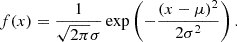
The main principles of the Γ-functions method are two functions, Γ1 and Γ2, which are used to identify vortex centers and boundaries, respectively. Graftieaux et al. (2001) defined these two functions as follows:
![$$ \begin{aligned} \begin{aligned}&\Gamma _1(P)=\frac{1}{N}\sum _S\frac{(\boldsymbol{PM} \wedge \boldsymbol{U_M})\cdot \boldsymbol{z}}{||\boldsymbol{PM}||\cdot || \boldsymbol{U_M} ||}=\frac{1}{N}\sum _S\sin (\theta _M),\\&\Gamma _2(P)=\frac{1}{N}\sum _S\frac{[\boldsymbol{PM} \wedge (\boldsymbol{U_M}- \boldsymbol{\tilde{U}_P})]\cdot \boldsymbol{z} }{|| \boldsymbol{PM} ||\cdot || \boldsymbol{U_M} - \boldsymbol{\tilde{U}_P}||}. \end{aligned} \end{aligned} $$](/articles/aa/full_html/2025/08/aa54524-25/aa54524-25-eq1.gif)
Here, P is a target point in the measurement domain and S is a two-dimensional region surrounding it, containing N pixels. In other words, S is the region used to calculate Γ1 and Γ2, and therefore N is equal to the square of the kernel size. M is a random point in S and z represents the unit vector perpendicular to the observational surface. The angle between UM (the velocity vector of point M) and PM (the vector from point P to point M) is denoted by θM. The symbols ∧, ⋅, and ∥ ⋅ ∥ represent the vector cross product, dot product, and norm, respectively. The local convection velocity around P is given by 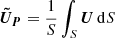 . Graftieaux et al. (2001) reported that |Γ1| reaches values ranging from 0.9 to 1 near the vortex center, while |Γ2| is equal to 2/π at the vortex boundaries. Based on these two parameters, the center and boundaries of each vortex can be decided.
2.2. Automated swirl detection algorithm
ASDA is an automated vortex identification algorithm based on the Γ-functions method. The algorithm consists of two essential steps for performing vortex identifications on a dataset from observations or simulations. The first step is to estimate the velocity field using FLCT (Welsch et al. 2004; Fisher & Welsch 2008). Liu et al. (2019b) developed an integrated Python wrapper for the FLCT code, which is available in their GitHubrepository1. Specifically, the pixel width of the Gaussian filter (sigma) is set to ten, and the low-pass spatial filtering (kr) and skip are set to None. Fisher & Welsch (2008) provided a more detailed explanation of other parameters not mentioned here. The next step is to apply the Γ-functions method (Graftieaux et al. 2001) to the velocity field estimated by FLCT.
Liu et al. (2019b) made some minor adjustments to the Γ1 and Γ2 functions. For each pixel P, they defined the two parameters as follows:
The symbols and vectors in Eq. (2) are similar to those in Eq. (1). More detailed interpretations of these functions can be found in previous studies (e.g., Liu et al. 2019a,b,c; Xie et al. 2025).
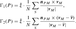
Figure 1 shows an example of a vortex V with its center P, rotation speed vrM, expansion speed veM, and speed vector vM at any point M in region S, which is used to calculate the Γ1 and Γ2 values at its central point P. We note that when ve is negative, it becomes the contraction speed vc. The quantities vr, ve, and v represent the average rotation speed, expansion speed, and speed vector of all points in S, centered on point P. The quantity  is defined as the average value of sin(θM) for all points M within the region S.
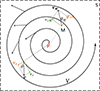 |
Fig. 1. An example vortex V with its center P. A point M is randomly chosen within the vortex V, with rotation speed vrM, expansion speed veM, and speed vector vM. The region S is used to calculate Γ1 and Γ2 values at the center P. The average rotation speed vr, expansion speed ve, and speed vector v of all points in S, centered on point P, are also shown. The quantity |

The quantity Γ1(P) is expressed as:
where  . Furthermore,
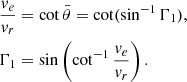
Therefore, if 0.89 is set as Γ1min, correspondingly,  . For a vortex whose
  , |Γ1| at its center will be less than 0.89, and thus it will not be detected as a vortex by ASDA. For different values of Γ1min, we can analyze their implications and identify the values of
  of vortices that may be excluded. This analysis contributes to subsequent sections of the paper.
2.3. Validation with synthetic data
To determine the optimal parameters of ASDA to detect vortices with more accuracy, we needed to compare the detection results with exact known results. Therefore, we applied ASDA to synthetic data for comparison, rather than to numerical simulation or observational data. In this study, we used Lamb-Oseen vortices (Saffman 1995) as the synthetic vortices.
Assuming the maximum rotation speed vmax and radius rmax of a Lamb-Oseen vortex, a point at a distance r away from the center has a rotation speed:
![$$ \begin{aligned} v_r=v_{\max }\Bigg (1 + \frac{1}{2\alpha }\Bigg )\frac{r_{\max }}{r}\Bigg [1 - \exp \Bigg (-\alpha \frac{r^2}{r_{\max }^2}\Bigg )\Bigg ], \end{aligned} $$](/articles/aa/full_html/2025/08/aa54524-25/aa54524-25-eq12.gif)
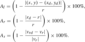
where α≈ 1.256. The expansion or contraction speed ve of the vortex can be arbitrarily assigned. For example, Liu et al. (2019b) set ve = 0.2vr in their synthetic data. In this way, we can intuitively associate a Lamb-Oseen vortex with the Γ1 value at the center. Figure 2 shows an example Lamb-Oseen vortex. The center of the Lamb-Oseen vortex C with coordinate (x, y) and the detected center Cd with coordinate (xd, yd) are located at the same pixel in panels (a) and (b) of Figure 2. Following Liu et al. (2019b), the location accuracy (Al), radius accuracy (Ar), and rotation speed accuracy (As) of the detected vortex are defined as
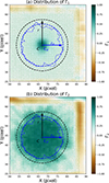 |
Fig. 2. Example of a synthetic vortex and the corresponding detected vortex by ASDA. (a) Velocity field of the region (green arrows) and the synthetic vortex edge (black dashed circle) with center C (black text) and radius r (black arrow and text). The edge and center of the detected vortex are shown as blue solid curves and a blue point (Cd), respectively, with effective radius rd (blue text and arrow). The effective edge (blue dashed circle) is determined by the effective radius rd. The background shows the distribution of Γ1. (b) Same as panel (a) but with the background showing the distribution of Γ2. |
Here, vr and vrd represent the actual and calculated rotation speeds of the Lamb-Oseen vortex.
3. Experiments and results
3.1. Optimal Γ1min
As mentioned in the introduction, there are discrepancies and uncertainties when choosing the value of Γ1min to determine whether a detected feature is a vortex or not. First, we refer to the approach of testing ASDA (with a kernel size of 7) using a series of synthetic data, as described in Liu et al. (2019b). We generated 1000 Lamb-Oseen vortices whose radii rmax and rotation speeds vmax follow the following Gaussian distribution:
Here, f(x) is the probability density of the variable x, μ is its expected value, and σ is the standard deviation. Based on the statistical results of detected photospheric vortices in Liu et al. (2019b), we set the expected radius of the vortices to μr = 7.2 pixels, with a standard deviation σr = 1.5 pixels. Similarly, the expected rotation speed was defined as μv = 0.17 pixels per frame with a standard deviation σv = 0.07 pixels per frame. For the expansion speed ve of each vortex, we set ve = κ ⋅ vr. Here, κ is a parameter that also follows a Gaussian distribution, with an expected value set to μκ = 0.9 and a standard deviation σκ = 0.2. Thus, according to the 3σ rule for Gaussian distributions, approximately 99.7% of data points fall within ±3σ of the mean, indicating that nearly all values of κ are concentrated between 0.3 and 1.5. This range is wide enough to represent most vortices. The generated vortices were then randomly divided into two equal groups: one rotating counterclockwise (positive rotation) and the other clockwise (negative rotation). A background noise map of 5000 × 5000 pixel2 was generated, with each pixel assigned a velocity with a random direction and a random magnitude between 0% and 20% of μv. Next, the 1000 vortices were randomly placed within this background noise map, ensuring no overlap among them. This process resulted in a synthetic velocity map, named synthetic data 1 (SD1), which closely resembles observational data. Next, we applied ASDA to SD1 using different values of Γ1min from 0.45 to 0.89 to detect vortices. This process was repeated 100 times. The detection results for vortices from SD1 with noise levels of 0 and 20% are shown in Tables 1 and 2.
Detection results of SD1 with a velocity noise level of 0.
Detection results of SD1 with a velocity noise level of 20%.
Tables 1 and 2 list the detection rate, false detection rate, location accuracy, radius accuracy and rotation speed accuracy of all detected vortices at velocity noise levels of 0 and 20% from SD1. There is little difference in results with Γ1min from 0.45 to 0.60: the detection rates and accuracies for the location, radius, and rotation speed all remain high. However, for both noise levels, the detection rates decrease slightly (3.4% in Table 1 and 8% in Table 2) when Γ1min increases from 0.60 to 0.65, and both detection rates drop rapidly when Γ1min exceeds 0.65. Note that the false detection rate is consistently zero with increasing Γ1min and the accuracies of location, radius, and rotation speed all remain high. This finding further supports the result of Liu et al. (2019b) that ASDA is unlikely to detect a vortex at a location where none exists.
As mentioned above, κ obeys the Gaussian distribution N(0.9, 0.22) for all vortices in SD1, and nearly all values of κ are between 0.3 and 1.5. This means that theoretically, |Γ1| values at vortex centers should be distributed from 0.55 (sin(cot−11.5)) to 0.96 (sin(cot−10.3)). Therefore, approximately 99.7% of vortices could be detected by ASDA with Γ1min = 0.55, and for any Γ1min ≤ 0.55, the detection rates should be very similar. This is consistent with the observations of Tables 1 and 2. It should also be noted that the detection rates only drop significantly when Γ1min exceeds 0.65, which may indicate that the optimal value for Γ1min is around 0.60 to 0.65. Moreover, to avoid randomness, we conducted two additional experiments by setting μr = 14.4 pixels with σr = 2.4 pixels, and μr = 3.6 with σr = 0.8 pixels, respectively. The results of these experiments are similar to those for SD1, suggesting that ASDA performs well in identifying vortices with different radii.
After considering the radii of the vortices, we varied the values of κ and conducted new experiments to explore how the ratio between expansion and rotation speeds affects the results. A new synthetic dataset, SD2, similar to SD1, was generated that also contains 1000 Lamb-Oseen vortices. The expected radius and standard deviation were set to μr = 7.2 pixels and σr = 1.5 pixels, respectively, and the expected rotation speed was defined as μr = 0.17 pixels with a standard deviation of σv = 0.07 pixels. However, for ve = κ ⋅ vr, κ was set to obey the Gaussian distribution N(0.5, 0.12) for all 1000 vortices in SD2 (compared to κ obeying N(0.9, 0.22) in SD1). Similarly, approximately 99.7% of values of κ are between 0.2 and 0.8, indicating that values of |Γ1| at vortex centers are mostly concentrated between 0.78 (sin(cot−10.8)) and 0.98 (sin(cot−10.2)). As expected, there is little difference between the detection rates with Γ1min ≤ 0.78, however, an obvious decrease occurs when Γ1min increases from 0.75 to 0.80. To further validate these observations, a further experiment was conducted with a larger κ, obeying the Gaussian distribution N(1.2, 0.22), with all other conditions being kept the same as in SD2, generating the synthetic data SD3. The detection results for SD3 with different Γ1min under the noise level of 20% are shown in Table 3.
Detection results of SD3 with a velocity noise level of 20%.
There is some commonality between the detection results under different conditions, as shown in Table 1, Table 2, and Table 3. The detection rates all exhibit the first “quick” decrease from Γ1min = 0.60 to Γ1min = 0.65. The detection rates decrease by 3.4% in Table 1, 8% in Table 2, and 12.2% in Table 3. According to Eq. (4), values of |Γ1| at the vortex centers in SD3 are mostly concentrated between 0.49 (sin(cot−11.8)) and 0.86 (sin(cot−10.6)). However, the detection rate is only 50.2% with Γ1min = 0.45, significantly less than 99.7%. This indicates that some vortices are detected as candidate vortices by the criterion Γ1min but are rejected by other criteria. Based on the methodology of ASDA described in Sect. 2.2, we speculate that the criterion on Γ2 may have also excluded some candidate vortices. To verify this, we sampled a small region (200 × 200 pixels2) of SD3 to compare the location distribution of vortices with the value distribution of Γ1 and Γ2.
There are a total of ten synthetic vortices in the 200 × 200 pixel2 region, which are marked using black numbers in the four panels of Figure 3. As shown in Figure 3a and c, vortices Nr. 1, 4, 5, 6, 7, 8 and 10 are not identified as vortices with Γ1min = 0.60 and 0.65, among which Nr. 1, 4, 6, 7 and 8 are also rejected by Γ2 (Fig. 3b and d). However, Nr. 5 and Nr. 10 satisfy the condition |Γ1|≥0.60 although they are not identified by |Γ1|≥0.65 and |Γ2|≥2/π. This indicates that if Γ1min is set at 0.60 or less, some vortices will be accepted by the Γ1 condition but rejected by the Γ2 condition. Although this has little influence on the detection results, it may cause a significant waste of computing resources for a large dataset.
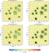 |
Fig. 3. Comparisons of detected results by ASDA under different criteria. Panels (a) and (b) show the distributions of Γ1 and Γ2 (backgrounds) in a 200 × 200 pixel2 region of SD2. Green arrows indicate the velocity field, and the numbers label the ten synthetic Lamb-Oseen vortices. Black dots in panel (a) mark points where |Γ1| ≥ 0.60, while black dots in panel (b) correspond to points where |Γ2| ≥ 2/π. Panels (c) and (d) are similar to (a) and (b), respectively, but the black dots show points where |Γ1| ≥ 0.65 and |Γ2| ≥ 2/π, respectively. Blue and red curves in these four panels represent the boundaries of vortices rotating counterclockwise and clockwise, respectively. |
Secondly, vortices Nr. 2 and 3 are detected as a positive vortex and a negative vortex, respectively, with Γ1min = 0.60. However, they are not detected by ASDA with Γ1min = 0.65, because the |Γ1| values of the points in vortices Nr. 2 and 3 are all less than 0.65, and no points are identified as their centers. Their boundaries are both detected successfully (see black dots of Nr. 2 and 3 in Fig. 3b and d) according to the Γ2 criterion (i.e., |Γ2| = 2/π at the vortex boundaries Graftieaux et al. 2001). Thus, vortices Nr. 2 and 3 are genuine vortices, but when Γ1min = 0.65 or larger, they would not be detected as vortices. In other words, setting Γ1min too high (0.65 or greater), results in missed detection of real vortices by ASDA, leading to an underestimation of their total number.
In conclusion, we can first determine whether a rotational structure is a real vortex based on the Γ2 criterion. If its boundaries where |Γ2| = 2/π are identified, an optimal Γ1min should be used to determine whether the candidate is a vortex or not. The above experiments with different vortex distributions and noise levels suggest that the optimal Γ1min should be between 0.60 and 0.65. To find the exact value of the optimal Γ1min, we applied ASDA with Γ1min = 0.45 (sufficiently small) to SD1 (ve = N(0.9, 0.22)⋅vr) and SD3 (ve = N(1.2, 0.22)⋅vr) with noise levels of 0 for both. This makes the value range of ve/vr (0.3 ∼ 1.8) wide enough to cover most of the distributions of ve/vr. Statistically, the minimum values of |Γ1| at vortex centers detected in SD1 and SD3 are 0.638 and 0.637, respectively. The values are both between 0.60 and 0.65, which can explain the rapid decreases from Γ1min = 0.60 to Γ1min = 0.65 in Tables 1, 2 and 3. Therefore, we suggest that the optimal value of Γ1min is 0.63, and we can detect almost all vortices by applying ASDA with Γ1min = 0.63. This optimal value of Γ1min is further tested and validated with numerical simulation and observational data in the remainder of this section.
3.2. Influence of the kernel size
After determining the optimal value of Γ1min as 0.63, in this subsection, we explore the influence of the kernel size (ks) in calculating Γ1 and Γ2. Liu et al. (2019b) specified N (ks2) as 49, indicating a kernel size of 7, and calculated Γ1 and Γ2 in a region of 7 × 7 pixel2 surrounding each target point. The above specification weakens vortices with radii smaller than four pixels, indicating that ASDA may fail to identify some small-scale vortices (radii smaller than four pixels) and so would underestimate the number of vortices.
Yuan et al. (2023) proposed the Advanced Γ Method (AGM) to identify vortices and used an adaptive version to optimize AGM for vortex identification. This adaptive version is based on a sequence of different kernel sizes, such as 3, 5, 7, 9, 11 and so forth. Yuan et al. (2023) noted that there are different values of Γ1 and Γ2 for the same point when using different kernel sizes for the calculation. For example, if |Γ1| of a point is calculated as less than Γ1min using ks = 7 but greater than Γ1min using ks = 9, then this point may be a potential vortex center and should not be omitted immediately. Therefore, Yuan et al. (2023) calculated the values of Γ1 with several kernel sizes (3, 5, 7, 9, and 11) and used the maximum |Γ1| in each pixel with different kernel sizes. Yuan et al. (2023) also suggest that varying the kernel size for each vortex provides better identification and leads to more accurate statistical results for the vortex parameters. However, experiments carried out by Yuan et al. (2023) used an arbitrary Γ1min = 0.75, and the influence of different kernel sizes on detection results with the optimal Γ1min = 0.63 requires further examination.
Next, we calculated Γ1 and Γ2 with kernel sizes = 3, 5, 7, 9, and 11. At each pixel, only the maximal values of |Γ1| and |Γ2| with different kernel sizes were combined. Vortex detection based on ASDA was then applied to these combined Γ1 and Γ2 values. We named this version variable Γ calculating method-origin (VGCM-o) and tested it with synthetic data using Γ1min = 0.63. According to Eq. (4), Γ1min = 0.63 corresponds to κ = ve/vr = 1.23, which means that vortices whose κ > 1.23 will not be detected by ASDA. Therefore, to avoid the potential influence of Γ1min, SD2 was the most suitable dataset to test VGCM-o with Γ1min = 0.63, because κ values of vortices in SD2 are mostly located between 0.2 and 0.8. The detection results for SD2 with noise levels ranging from 0 to 20% are shown in Table 4.
Detection results of SD2 using VGCM-o with Γ1min = 0.63.
Table 4 shows that the detection maintains high accuracy for the location, radius, and rotation speed of vortices at a noise level of 0. However, when noise is present, even with a noise level of only 5%, the detection rate exceeds 100% and false detections occur. The location accuracy becomes negative, indicating that the detected vortex center is outside the synthetic vortex. The radius accuracy and the rotation speed accuracy remain high. To confirm these findings, we also varied the radii of vortices in SD2 to larger and smaller values and obtained similar detection results. This suggests that VGCM-o performs well in identifying vortices when there is no noise, but detects false vortices and yields unreliable vortex centers when noise is present in the dataset, a situation that is very common in observational data.
To investigate the reasons for the poor behavior of VGCM-o with noisy data and to search for a better method to calculate Γ1 and Γ2, we recalculated the values of Γ1 and Γ2 in SD2 using different single kernel sizes (ranging from 3 to 15) and applied the detection steps of ASDA to these Γ1 and Γ2 values, also with Γ1min = 0.63.
The detection results are shown in Table 5. We find that the detection rate is highest when ks = 9 and the detection rate decreases if ks increases (11, 13, and 15) or decreases (5 and 7). Moreover, only when ks = 3, does the detection rate exceed 100%, and false vortices are detected, with very poor location, radius, and rotation speed accuracies. It is clear that the detection results with VGCM-o and ks = 3 are similar, and therefore the poor detection results with VGCM-o are attributable to ks = 3. To verify this, we revised VGCM-o by removing ks = 3 when calculating Γ1 and Γ2.
Detection results of SD2 with a velocity noise level of 20% using different kernel sizes.
In Table 5, VGCM-1 uses kernel sizes of 5, 7, and 9; VGCM uses kernel sizes of 5, 7, 9, and 11; and VGCM-2 uses kernel sizes of 5, 7, 9, 11, and 13. For these three combinations of kernel sizes, the detection rates are all at high and reasonable levels (< 100%), with high location, radius and rotation speed accuracies. False vortices are not detected, indicating that the detection results are improved after excluding ks = 3. Moreover, the results of VGCM, VGCM-1, and VGCM-2 are all better than the results of using any single kernel size, demonstrating that the variable Γ-functions method contributes to more accurate detection of vortices. Considering that the detection rates of VGCM and VGCM-2 are the same and both 0.3% higher than the detection rate of VGCM-1, VGCM (with kernel sizes of 5, 7, 9, and 11, and costing less computation power compared to VGCM-2) is found to be the best for SD2, whose vortex radii follow the Gaussian distribution of N(7.2, 1.62).
Next, we varied the radii of the vortices in SD2 to smaller and larger values following N(3.6, 0.82) and N(14.4, 2.42), respectively, and repeated the above experiments. Both results support our findings that the poor detection results with VGCM-o result from ks = 3. When using only a single kernel size, ks = 5 is the best choice for smaller vortices, whereas ks = 19 is the best for larger vortices. This suggests that the best single kernel size is always close to the average radius of vortices in the dataset. Although we also find that a VGCM containing this best single kernel size performs better, the improvement compared to VGCM (kernel sizes = 5, 7, 9, and 11) is very little (∼1%) but requires significantly more computational resources. Moreover, because it is impossible to know the average radius of vortices in observational data, we cannot adjust the VGCM by selecting specific kernel sizes. Therefore, in practice, VGCM (kernel sizes = 5, 7, 9, and 11) is most suitable for accurate vortex detection while avoiding false detections.
3.3. Validation with numerical simulation data
3.3.1. Photosphere
In Sects. 3.1 and 3.2, we concluded that the VGCM is a suitable approach to calculate Γ1 and Γ2, and Γ1min = 0.63 is a more practical choice than 0.89 (Liu et al. 2019b) or 0.75 (Yuan et al. 2023). We name this version of the improved ASDA, which calculates Γ1 and Γ2 using a VGCM and detects vortices with Γ1min = 0.63, the Optimized ASDA. We note that the above results are obtained by experiments with various synthetic data, and whether the Optimized ASDA can be applied to observational data remains to be studied. Therefore, before applying the Optimized ASDA to observational data, we firstly tested it with advanced numerical simulation obtained with the CO5BOLD code (Freytag et al. 2012). This code has been widely used to model stellar atmospheres, such as those of the Sun, solar-type stars, red giants, and white and brown dwarfs (Straus et al. 2017). Different solvers, such as a hydrodynamic module or a magnetohydrodynamic module, and radiative transfer schemes, can be chosen to simulate variable situations, due to a modular construction of the code (Straus et al. 2017).
In this subsection, we use data from the radiative MHD code to simulate the surface layers of the Sun. The simulation was based on a relaxed, purely hydrodynamical model with an initial vertical and homogeneous magnetic field of 50 G. The HLLMHD solver (Harten et al. 1983; Schaffenberger et al. 2005, 2006) was used to ensure the positivity of the gas pressure. The magnetic and plasma boundary conditions were both periodic at the sides, while the magnetic field was enforced to be vertical at the top and bottom of the box. The Cartesian simulation box had a grid spacing of 960 × 960 × 280 grid cell3, with a cell size of 10 km in each spatial direction, representing a total size of 9.6 × 9.6 × 2.8 Mm3. The height of the box (labeled as z) ranged from −1240 km to 1560 km, with z = 0 km representing the average optical depth τ500 = 1. Therefore, the simulation domain encompassed layers near the solar surface, including the convection zone, photosphere, and up to the middle chromosphere (Cuissa & Steiner 2024). This simulation started at t = 0 s and ran for about 7680 s (i.e., about 2.1 h), with a cadence of 240 s. Discarding the first 1600 s of the simulation (typically the time for the initial magnetic field to relax), 26 data cubes were obtained, from t = 1680 s to t = 7680 s.
Cuissa & Steiner (2022) proposed an innovative and automated method for vortex identification, named SWIRL. This algorithm mainly involves two steps: (1) estimating the vortex center map for each image and (2) clustering the estimated centers and identifying the vortices. For a point with coordinate (x, y) and velocity (vx, vy), the vorticity ω, the velocity gradient tensor 𝒰, the real eigenvector ur, the swirling strength λ, and the Rortex R can be computed based on the definitions in Cuissa & Steiner (2022). The radial direction and curvature radius of this point can then be calculated, which determine its estimated vortex center (EVC).
Applying this method, one obtains the EVC map for each image. Furthermore, based on the EVC maps, the number of EVCs in each grid cell (EVC density) can be counted using the clustering by fast search and finding of density peaks (CFSFDP) algorithm proposed by Rodriguez & Laio (2014). Clustered EVCs are then obtained based on specific criteria (see details in Cuissa & Steiner 2022), and candidate vortices are identified. After noise removal, identified vortices and noisy grid cells are distinguished. Several properties of each vortex can then be obtained, including its center coordinate, effective radius defined by Cuissa & Steiner (2022), and rotational direction (counterclockwise or clockwise). More details about the SWIRL method can be found in Cuissa & Steiner (2022). Cuissa & Steiner (2024) recommended a set of SWIRL algorithm parameters for detecting vortices in the above simulation data cubes. Next, we compared the vortex detection results from the Optimized ASDA and SWIRL applied to the photospheric velocity field of the numerical simulation by Cuissa & Steiner (2022).
Panels (a) and (b) in Figure 4 show an example Bz from the first frame of the CO5BOLD simulations at the photosphere. Here, when applying the Optimized ASDA, we continued to use the VGCM to calculate Γ1 and Γ2 but varied the value of Γ1min from 0.45 to 0.89 to explore how vortex detection would be affected with different Γ1min criteria. Detection results from the Optimized ASDA and SWIRL are shown in Figure 5.
 |
Fig. 4. Example frames and the detected vortices of CO5BOLD simulation data and SST observational data. Panels (a) and (c) show the first frames of the CO5BOLD simulation and SST observational data, displaying the Bz from CO5BOLD and the photospheric intensity from SST, respectively. In panel (a), cyan and black curves denote boundaries of counterclockwise and clockwise vortices detected by SWIRL, while in panel (c), blue and red curves indicate the corresponding vortices detected by ASDA. Panels (b) and (d) show close-up views of the purple box in (a) and the yellow box in (c), respectively. Green arrows in (b) and (d) represent the velocity field. |
In Figure 5(a), the blue curve shows the average number of photospheric vortices per frame detected by the Optimized ASDA for different Γ1min values from the 26 photospheric simulation data cubes. The number decreases almost linearly as Γ1min increases. The number of vortices detected by SWIRL is indicated by the horizontal red line. The purple curve shows the number of vortices detected by both the Optimized ASDA and SWIRL. It is evident that when Γ1min is less than 0.5, almost all vortices detected by SWIRL are also detected by the Optimized ASDA. However, the number of overlapping vortices decreases slowly with increasing Γ1min when Γ1min is less than 0.65, above which, the overlapping number decreases rapidly. To clarify the decreasing trend in the number of overlapping vortices, we calculated the overlap rates, defined as the percentage of overlapping vortices over the total number of vortices detected by SWIRL (green curve in Fig. 5a). Figure 5(b) shows the slope at each point along the green curve in Figure 5(a). The slopes of the overlap rate at Γ1min = 0.45, 0.63, and 0.80 are −0.07, −0.53, and −3.56, respectively. The two bright teal dotted vertical lines in panels (a) and (b) both correspond to Γ1min = 0.63. The overlap rate decreases more sharply (panel a) and more rapidly (panel b) from Γ1min = 0.63 to 0.80 than from Γ1min = 0.45 to 0.63. This suggests that most vortices detected by SWIRL can also be identified by the Optimized ASDA with Γ1min = 0.63 or less. However, as Γ1 increases further, the Optimized ASDA misses a significant number of vortices, and thus underestimates the number of vortices in the data. These results are consistent with those obtained from the synthetic data in Sect. 3.1 and Sect. 3.2, further supporting that 0.63 is an optimal choice for Γ1min.
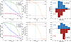 |
Fig. 5. Comparisons between the detection results obtained from the Optimized ASDA and SWIRL with numerical simulations. Panels (a), (b), and (c) show detection results from the photospheric simulation data. In panel (a), the blue curve and red horizontal line show the average numbers of vortices per frame detected by the Optimized ASDA and SWIRL, respectively. The purple curve shows the number of overlapping vortices detected by the Optimized ASDA and SWIRL, while the green curve indicates the corresponding overlapping rate. Panel (b) depicts the slope of each point of the green curve in panel (a). Panel (c) presents histograms of the radius distributions for overlapping vortices detected by the Optimized ASDA and SWIRL. Panels (d), (e), and (f) provide similar information for chromospheric simulation data. |
We also note that Liu et al. (2019b) and Cuissa & Steiner (2022) computed the effective radius of vortices using the same method, which is defined as the radius of a circle having the same area as the vortex:

Here, Aeff is the effective area of a vortex, determined by the number of grid cells within the vortex and the cell size. Therefore, we focus on the distributions of the radii of vortices detected by both the Optimized ASDA and SWIRL. These distributions are shown in Figure 5(c), which reveals little difference between the radii distributions of vortices detected by the Optimized ASDA and SWIRL. The expected values of the vortex radius detected by the Optimized ASDA and SWIRL are 71.05 km and 61.37 km, with corresponding standard deviations of 19.88 km and 21.90 km, respectively. These results suggest that the Optimized ASDA with Γ1min = 0.63 can not only detects most vortices identified by SWIRL (and additional vortices not detected by SWIRL) but also performs very well in determining the radii of the detected vortices. These findings further support our previous findings regarding the Optimized ASDA from synthetic data.
3.3.2. Chromosphere
In this subsection, we explore the performance of the Optimized ASDA by applying it to chromospheric data from the previously described numerical simulation. The chromospheric simulation data cubes cover the same horizontal domain and were sampled at the same time as those chosen in Sect. 3.3.1. However, the height corresponding to the bottom of the chromosphere is at z = 700 km, higher than the height (z = 100 km) of photospheric data cubes in Sect. 3.3.1.
The results are similar to those obtained from the photospheric simulation data cubes, and are shown in Figure 5(d)–(f). In panel (d), the blue curve, representing the number of vortices detected by the Optimized ASDA, also shows an almost linear decrease with increasing values of Γ1min. The purple and green curves closely resemble the corresponding curves in panel (a), although more vortices are detected by both the Optimized ASDA and SWIRL in the chromospheric data. Panel (e), analogous to panel (d), depicts the slope of each point along the green curve in panel (d), and the slope of overlap rates are −0.07, −0.53, and −3.70 at Γ1min = 0.45, 0.63, and 0.80, respectively. The difference between the slopes from Γ1min = 0.45 to 0.63 is negligible compared to the variation from Γ1min from 0.63 to 0.80. This suggests that the chromospheric detection results are consistent with those from the photospheric simulation data and further supports the conclusion that 0.63 is an optimal value for Γ1min. Moreover, the radii of overlapping vortices detected by the Optimized ASDA appear to be slightly smaller than those detected by SWIRL, as shown in Figure 5(f). The expected values of the radii detected by the Optimized ASDA and SWIRL are 98.17 km and 92.97 km, with corresponding standard deviations of 37.78 km and 18.02 km, respectively.
Comparing vortices detected from the photosphere and chromosphere suggests that there are more vortices in the solar chromosphere than in the photosphere in the numerical simulation. This is consistent with the observational fact that ASDA detects more vortices in the chromospheric observations than in photospheric observations (Liu et al. 2019c). Cuissa & Steiner (2024) suggests that the growth of vortex radii could be explained by the steep decrease in mass density from the photosphere to the chromosphere, which results in expansion of the plasma ascending into the chromosphere (Nordlund et al. 1997).
In summary, based on the above results and comparisons using data from the CO5BOLD numerical simulation, we conclude that 0.63 for Γ1min is also an optimal choice for detecting vortices in numerical simulation data.
3.4. Validation with observational data
The data analyzed in this subsection consists of high-resolution photospheric images centered on the Fe I 630.25 nm spectral line, with a spectral window width of 0.45 nm. These observations were acquired using the CRisp Imaging SpectroPolarimeter (CRISP; Scharmer 2006; Scharmer et al. 2008) on the Swedish 1-meter Solar Telescope (SST; Scharmer et al. 2003). Conducted on July 7, 2019, between 08:23:36 UT and 08:39:18 UT, the observations targeted a quiet-Sun region near the central meridian. The field of view (FOV), centered at (xc = 0″, yc = −300″), covered an area of 56.5″ × 57.5″. The pixel size of the data is 0.059″ (∼43.6 km), with a spatial resolution estimated to be at least 87.2 km, corresponding to twice the pixel size. The images were taken with an average cadence of 4.2 seconds, and the FOV was rotated 70 degrees clockwise relative to the Sun’s north pole.
Figure 4 also presents an example photospheric intensity map from SST observations in panel (c). Blue and red curves outline the boundaries of vortices detected by ASDA. Panel (d) shows a close-up view of the yellow box in panel (c).
Similar to Figure 5, Figure 6 shows the comparison between vortices detected by ASDA and SWIRL from the SST observations. Figure 6(b) shows the slope at each point along the green curve in panel (a), with slopes at Γ1min = 0.45, 0.63, and 0.80 as −0.03, −0.48, and −4.44, respectively. The rapid drop in slope from Γ1min = 0.63 to 0.80 is also observed, similar to Figure 5(b) and (e) for the numerical simulation data. Additionally, the radii detected by the Optimized ASDA and SWIRL exhibit nearly identical distributions, with similar expected values (322.24 km vs. 300.46 km) and standard deviations (67.54 km vs. 52.29 km), as shown in Figure 6(c). These results are highly consistent with the vortex detection results from numerical simulation data in Sect. 3.3, indicating that the Optimized ASDA with Γ1min = 0.63 also performs well in detecting vortices from solar observational data.
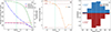 |
Fig. 6. Comparisons between the detection results obtained from the Optimized ASDA and SWIRL using observational data. Similar to Fig. 5 but applied to observational datasets. |
We also explored the influence of kernel size on vortex detection using both numerical simulation data and observational data. We detect vortices from Γ1 and Γ2 calculated with VGCM, VGCM-o, and a single kernel size 7, all using the optimal Γ1min = 0.63. The results are similar; here, we take the results from the photospheric simulation data as an example. There are approximately 9% more vortices detected with VGCM and VGCM-o than with a single kernel size of 7, and correspondingly, more vortices detected by SWIRL overlap with those detected with VGCM and VGCM-o. These findings support the results in Sect. 3.2, indicating that the Variable Γ Calculating Method is more suitable than using a single kernel size for calculating Γ1 and Γ2. Furthermore, the number of vortices detected with VGCM-o is slightly higher (∼2%) than with VGCM, but the number of overlapping vortices with SWIRL is identical. This indicates that it is very likely that the additional vortices detected with VGCM-o are false detections, supporting our previous conclusions that VGCM is more accurate in detecting vortices than VGCM-o.
4. Conclusions and discussion
In this paper, we employed the automated swirl detection algorithm (ASDA), an automated algorithm based on the Γ-functions method, to detect vortices from synthetic data generated under diverse conditions. We also aimed to improve the Γ-functions method for vortex identification. We analyzed the effect of varying the values of Γ1min, which determines the centers of vortices, and tested various approaches for calculating Γ1 and Γ2 to identify both the optimal value of Γ1min and the most effective method to calculate Γ1 and Γ2. The improved version of ASDA is referred to as the Optimized ASDA. In this section, we briefly summarize our results and discuss the potential implications of Optimized ASDA.
In the first stage of this work, we fixed the kernel size at ks = 7 to calculate Γ1 and Γ2 and applied ASDA with different values of Γ1min to synthetic data 1 (SD1). Regardless of whether the velocity noise was 0 or 20%, the detection rates showed little difference when Γ1min≤ 0.60, but decreased rapidly once Γ1min > 0.60. For SD1, κ, defined as κ = ve/vr in Sect. 3.1, was set to follow the Gaussian distribution N(0.9, 0.22). Theoretically, about 99.7% of vortices could be detected by ASDA with Γ1min equal to 0.55 or less, based on the deductions in the third paragraph of Sect. 2, which was confirmed by the experimental results shown in Tables 1 and 2. By exploring the variation of vortex radii (both larger and smaller) in SD1 and repeating the experiments, we found similar results, indicating that ASDA performs well in detecting vortices with different radii.
By changing κ to smaller (N(0.5, 0.12)) and larger (N(1.2, 0.22)) values, we constructed two new datasets, SD2 and SD3. Similar results were found: when Γ1min is less than 0.60, the detection rate by ASDA is almost invariable. It is worth noting that the detection rate (∼50%) of vortices at Γ1min = 0.45 on SD3 with a noise level of 20% is lower than expected (99.7%). By studying an example region in SD3 with ten synthetic vortices, we found that some candidates were excluded by the Γ2 criterion when Γ1min was set too low. These results suggest that negative impacts on the performance of ASDA would be introduced with excessively large or small values of Γ1min. Further tests on additional synthetic data revealed an optimal value of 0.63 for Γ1min.
Next, we fixed the Γ1min at 0.63 and searched for an appropriate method to calculate Γ1 and Γ2. Motivated by the adaptive version of the Advanced Γ Method proposed by Yuan et al. (2023), we presented the Variable Γ Calculating Method (VGCM) to calculate the two Γ functions. To determine the best method, we conducted comparative experiments on SD2 using different calculation method: single kernel sizes (ranging from 3 to 15) and several versions of the Variable Γ Calculating Method (VGCM-o, VGCM-1, VGCM, and VGCM-2), with results shown in Table 4. False vortices were detected only when using a single kernel size of ks = 3 and VGCM-o (kernel sizes = 3, 5, 7, 9, and 11), indicating that ks = 3 resulted in poor detection results. Moreover, by comparing the detection results with other methods, as shown in Table 4, we found that the Variable Γ Calculating Method performed better than single kernel size, and VGCM (with kernel sizes = 5, 7, 9, and 11) required less computing resources than VGCM-1 and VGCM-2, while still achieving similar performance in detecting vortices in SD2. Similar results were obtained when varying the radii of vortices in SD2 to larger and smaller values. These results suggest that VGCM is the most suitable method for calculating Γ1 and Γ2.
After establishing that 0.63 is the optimal value of Γ1min and VGCM (kernel sizes = 5, 7, 9, and 11) is more appropriate for calculating Γ1 and Γ2, ASDA can be optimized for more accurate vortex identification, referred to as Optimized ASDA. To validate the reliability of Optimized ASDA, we applied it to detect small-scale vortices in both numerical simulation data of the solar atmosphere from the radiative MHD CO5BOLD code and observational photospheric data from SST. The comparison results are all similar and consistent with the conclusions in Sect. 3.1 and Sect. 3.2, confirming that the choice 0.63 of Γ1min and the application of the VGCM to calculate Γ1 and Γ2 are both more suitable than the original ASDA. However, we noted that the numbers of vortices detected by the Optimized ASDA were consistently higher than those detected by SWIRL, showing 39.8%, 80%, and 91.3% more vortices for the photospheric and chromospheric simulations, and the SST photospheric observations, respectively (see Fig. 5a, d and Fig. 6a). A possible reason is that SWIRL missed some vortices. Cuissa & Steiner (2022) and Cuissa & Steiner (2024) note two drawbacks of SWIRL: (1) the detection is not strictly Galilean invariant, meaning some vortices with rotation speeds comparable to the flow speeds could be missed by SWIRL. They also note that this shortcoming should not affect photospheric vortices because they are predominantly rooted in intergranular lanes and move slowly relative to the vortical flow speed (Tziotziou et al. 2023). (2) The parameters for clustering and detection in SWIRL require adjustments when applied to different data.
The two aforementioned drawbacks of SWIRL could result in the underestimation of vortex counts, but whether the additional vortices detected by the Optimized ASDA in Figure 5(a), (d) and Figure 6(a) are true vortices requires further exploration. Because the optimized ASDA may overestimate vortex numbers, this could explain why it detects more vortices overall.
The top panel of Figure 7 shows a 2 × 2 Mm2 region of the photospheric numerical simulation domain from CO5BOLD. Most vortices are identified by both methods, with similar effective radii, consistent with the similar vortex radius distributions in Figure 5(c). However, regions labeled R1, R2, and R4 (outlined in gray) contain vortices detected only by the Optimized ASDA. The middle and bottom panels of Figure 7 provide close-up views of the three regions. In R1, the positive vortex identified by the Optimized ASDA appeared to be an actual vortex, yet it was not identified by SWIRL. Similar omissions occur in R2 and R4, suggesting that SWIRL overlooks some true vortices detected by the Optimized ASDA, explaining the number gaps in Figure 5(a), (d), and Figure 6(a). However, the counterclockwise vortex in R2 appears questionable based on the streamline plot, while the other clockwise vortex is genuine. This result further supports earlier concerns that the Optimized ASDA could detect some false vortices.
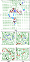 |
Fig. 7. Example vortices detected by the Optimized ASDA and SWIRL. Top panel: A small region of the CO5BOLD photospheric simulation domain. Green arrows represent the velocity field. Vortices detected by the Optimized ASDA and SWIRL that rotate counterclockwise are shown in blue and cyan, respectively. Clock-wise rotating vortices are shown in red (Optimized ASDA) and black (SWIRL). Bottom panel: Close-up views of four rectangular regions outlined by grey squares in the top panel. |
The boundary of the vortex detected by the Optimized ASDA in panel R4 does not conform closely to the velocity field (the red dotted circle seems more suitable). This suggests that the algorithm for determining vortex boundaries by the Optimized ASDA still requires improvement. In addition, a vortex identified by SWIRL (outlined by the black circle in Fig. 7R3) is detected as two separate vortices by the Optimized ASDA. However, examination of the velocity field reveals that the vortex identified by SWIRL is not genuine. The oval vortex at the top left and another at the bottom right, detected by the Optimized ASDA, are more consistent with the actual velocity field. These observations suggest that the Optimized ASDA outperforms SWIRL in detecting nonstandard-shaped vortices and in estimating the number of vortices in the solar atmosphere. It is worth noting that, noise was inserted into the velocity map to generate the synthetic data in this study. However, whether such synthetic data are well suited for generating nonstandard vortices (e.g., vortices detected by the Optimized ASDA in Fig. 7 R3) remains unclear. Future work focusing on a more detailed analysis of nonstandard vortices could lead to further improvement of ASDA and other vortex identification methods.
Liu et al. (2019c) found that abundant photospheric vortices excite Alfvén pulses, which propagate upward and carry energy flux into the upper chromosphere. They noted that the energy flux (FA) carried into the upper chromosphere by a single Alfvén pulse is estimated to be 1.9–7.7 kW m−2. The average energy flux ( ) is defined as
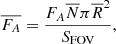
where  and
and  are the average number of vortices in each frame and vortex effective radius. The area of the FOV of the observation is represented by SFOV. We employed the original ASDA with Γ1min = 0.89 and the Optimized ASDA with Γ1min = 0.63 to the SST observations described in Sect. 3.4. On average, 39.6 and 308 vortices were detected by the original ASDA and the Optimized ASDA, respectively, withcorresponding average vortex radii of 308 km and 271 km. Therefore, using Eq. (9), the resulting
  is approximately 12.6–51.2 W m−2 and 75.9–308.3 W m−2 for the original ASDA and the Optimized ASDA, respectively. The former value is insufficient to balance the local radiative energy losses (∼100 W m−2) (Withbroe & Noyes 1977) in quiet-Sun regions. As previously noted, the Optimized ASDA may overestimate the number of vortices, while SWIRL may underestimate it. Thus, the energy flux (75.9–308.3 W m−2) estimated using the Optimized ASDA can be viewed as an upper limit of the flux supplied by the photospheric vortices. A lower limit of approximately 39.4–160.2 W m−2 is provided based on the number (160) of vortices identified by SWIRL. These results from the Optimized ASDA and SWIRL suggest that the average energy flux related to photospheric vortices is very likely sufficient to balance the energy losses. This further supports the conclusion that prevalent photospheric vortices could play significant roles in heating the upper atmosphere (e.g., Shelyag et al. 2013; Chmielewski et al. 2014; Mumford et al. 2015; Mumford & Erdélyi 2015; Liu et al. 2019c; Battaglia et al. 2021).
The Γ-functions method (and related automated algorithms, such as ASDA) for vortex identification depends heavily on the estimated horizontal velocity field. All methods used to calculate horizontal velocity fields all have their drawbacks. For example, the most common technique, FLCT, which we used in this work, should be applied with caution when estimating granular and subgranular flows (Tremblay et al. 2018; Cuissa & Steiner 2024). Moreover, Verma et al. (2013) and Liu et al. (2019b,c) showed that FLCT underestimates the horizontal velocity field by a factor of approximately three and influences the characteristics of detected vortices, such as the rotation and expansion speeds. In this study, synthetic data were used to improve the Γ-functions method. Therefore, our results are general and independent of the velocity estimation method.
Given the significant influence of the reconstructed velocity fields, a key direction of future work is to evaluate the reliability of different velocity estimation methods and to identify more reliable approaches for different observations.
One of our recent studies (Liu et al. 2025) used a neural network technique trained on high-resolution data (with a pixel size of ∼12 km, comparable to the diffraction limit of the Daniel K. Inouye Solar Telescope, DKIST, Rimmele et al. 2020) from realistic radiative numerical simulations of the solar photosphere. The built neural network model performs significantly better than FLCT at these small scales. Further investigation is warranted to determine how these different methods of estimating the photospheric horizontal velocity fields influence vortex detection by the Optimized ASDA.
Acknowledgments
We thank Dr. Fabio Riva in Istituto ricerche solari Aldo e Cele Daccò (IRSOL) for the source of the CO5BOLD simulation data. We acknowledge the support from the Strategic Priority Research Program of the Chinese Academy of Science (Grant No. XDB0560000) and the National Natural Science Foundation (NSFC 42188101, 12373056). R.E. is grateful to Science and Technology Facilities Council (STFC, grant No. ST/M000826/1) UK, acknowledges NKFIH (OTKA, grant No. K142987 and Excellence Grant, grant nr TKP2021-NKTA-64) Hungary and PIFI (China, grant number No. 2024PVA0043) for enabling this research. This work was also supported by the International Space Science Institute project (ISSI-BJ ID 24-604) on “Small-scale eruptions in the Sun”.
References
- Battaglia, A. F., Cuissa, J. R. C., Calvo, F., Bossart, A. A., & Steiner, O. 2021, A&A, 649, A121 [NASA ADS] [CrossRef] [EDP Sciences] [Google Scholar]
- Chmielewski, P., Murawski, K., & Solov’ev, A. A. 2014, RAA, 14, 855 [Google Scholar]
- Cuissa, J. C., & Steiner, O. 2022, A&A, 668, A118 [NASA ADS] [CrossRef] [EDP Sciences] [Google Scholar]
- Cuissa, J. C., & Steiner, O. 2024, A&A, 682, A181 [NASA ADS] [CrossRef] [EDP Sciences] [Google Scholar]
- Fisher, G., & Welsch, B. 2008, ASP Conf. Ser., 383, 373 [NASA ADS] [Google Scholar]
- Freytag, B., Steffen, M., Ludwig, H.-G., et al. 2012, J. Comput. Phys., 231, 919 [Google Scholar]
- Giagkiozis, I., Fedun, V., Scullion, E., Jess, D. B., & Verth, G. 2018, ApJ, 869, 169 [NASA ADS] [CrossRef] [Google Scholar]
- Graftieaux, L., Michard, M., & Grosjean, N. 2001, Meas. Sci. Technol., 12, 1422 [CrossRef] [Google Scholar]
- Harten, A., Lax, P. D., Leer, B. V., 1983, SIAM Rev., 25, 35 [CrossRef] [Google Scholar]
- Jiang, M., Machiraju, R., & Thompson, D. 2005, Visualization Handbook (Butterworth-Heinemann), 295 [Google Scholar]
- Kesri, K., Dey, S., Chatterjee, P., & Erdelyi, R. 2024, ApJ, 973, 49 [Google Scholar]
- Kitiashvili, I., Kosovichev, A., Lele, S., Mansour, N., & Wray, A. 2013, ApJ, 770, 37 [Google Scholar]
- Li, X., Morgan, H., Leonard, D., & Jeska, L. 2012, ApJ, 752, L22 [NASA ADS] [CrossRef] [Google Scholar]
- Liu, J., Zhou, Z., Wang, Y., et al. 2012, ApJ, 758, L26 [NASA ADS] [CrossRef] [Google Scholar]
- Liu, C., Gao, Y., Tian, S., & Dong, X. 2018, Phys. Fluids, 30 [Google Scholar]
- Liu, J., Carlsson, M., Nelson, C. J., & Erdélyi, R. 2019a, A&A, 632, A97 [NASA ADS] [CrossRef] [EDP Sciences] [Google Scholar]
- Liu, J., Nelson, C. J., & Erdélyi, R. 2019b, ApJ, 872, 22 [Google Scholar]
- Liu, J., Nelson, C. J., Snow, B., Wang, Y., & Erdélyi, R. 2019c, Nat. Commun., 10, 3504 [Google Scholar]
- Liu, J., Xie, Q., Zhong, C., et al. 2025, A&A, submitted [Google Scholar]
- Moll, R., Cameron, R., & Schüssler, M. 2011, A&A, 533, A126 [NASA ADS] [CrossRef] [EDP Sciences] [Google Scholar]
- Mumford, S., & Erdélyi, R. 2015, MNRAS, 449, 1679 [NASA ADS] [CrossRef] [Google Scholar]
- Mumford, S., Fedun, V., & Erdélyi, R. 2015, ApJ, 799, 6 [NASA ADS] [CrossRef] [Google Scholar]
- Murawski, K., Kayshap, P., Srivastava, A. K., et al. 2018, MNRAS, 474, 77 [NASA ADS] [CrossRef] [Google Scholar]
- Muthsam, H., Kupka, F., Löw-Baselli, B., et al. 2010, New Astron., 15, 460 [Google Scholar]
- Nordlund, A., Spruit, H., Ludwig, H.-G., & Trampedach, R. 1997, A&A, 328, 229 [Google Scholar]
- November, L. J., & Simon, G. W. 1988, ApJ, 333, 427 [Google Scholar]
- Panesar, N., Innes, D. E., Tiwari, S., & Low, B.-C. 2013, A&A, 549, A105 [NASA ADS] [CrossRef] [EDP Sciences] [Google Scholar]
- Parker, E. 1983, ApJ, 264, 642 [Google Scholar]
- Pettit, E. 1932, ApJ, 76, 9 [CrossRef] [Google Scholar]
- Pike, C., & Mason, H. 1998, Sol. Phys., 182, 333 [Google Scholar]
- Ramos, A. A., Requerey, I., & Vitas, N. 2017, A&A, 604, A11 [NASA ADS] [CrossRef] [EDP Sciences] [Google Scholar]
- Rieutord, M., Roudier, T., Roques, S., & Ducottet, C. 2007, A&A, 471, 687 [NASA ADS] [CrossRef] [EDP Sciences] [Google Scholar]
- Rimmele, T. R., Warner, M., Keil, S. L., et al. 2020, Sol. Phys., 295, 172 [Google Scholar]
- Rodriguez, A., & Laio, A. 2014, Science, 344, 1492 [NASA ADS] [CrossRef] [Google Scholar]
- Saffman, P. G. 1995, Vortex Dynamics (Cambridge University Press) [Google Scholar]
- Scalisi, J., Oxley, W., Ruderman, M. S., & Erdélyi, R. 2021, ApJ, 911, 39 [NASA ADS] [CrossRef] [Google Scholar]
- Scalisi, J., Ruderman, M. S., & Erdélyi, R. 2023, ApJ, 951, 60 [Google Scholar]
- Schaffenberger, W., Wedemeyer-Böhm, S., Steiner, O., & Freytag, B. 2005, in Chromospheric and Coronal Magnetic Fields, 596 [Google Scholar]
- Schaffenberger, W., Wedemeyer-Böhm, S., Steiner, O., & Freytag, B. 2006, in Solar MHD Theory and Observations: a High Spatial Resolution Perspective, 354, 345 [Google Scholar]
- Scharmer, G. 2006, A&A, 447, 1111 [NASA ADS] [CrossRef] [EDP Sciences] [Google Scholar]
- Scharmer, G. B., Bjelksjo, K., Korhonen, T. K., Lindberg, B., & Petterson, B. 2003, in Innovative Telescopes and Instrumentation for Solar Astrophysics, 4853, 341 [NASA ADS] [CrossRef] [Google Scholar]
- Scharmer, G. B., Narayan, G., Hillberg, T., et al. 2008, ApJ, 689, L69 [Google Scholar]
- Shelyag, S., Cally, P. S., Reid, A., & Mathioudakis, M. 2013, ApJ, 776, L4 [Google Scholar]
- Shetye, J., Verwichte, E., Stangalini, M., et al. 2019, ApJ, 881, 83 [Google Scholar]
- Silva, S. S., Fedun, V., Verth, G., Rempel, E. L., & Shelyag, S. 2020, ApJ, 898, 137 [NASA ADS] [CrossRef] [Google Scholar]
- Silva, S. S., Verth, G., Rempel, E. L., et al. 2021, ApJ, 915, 24 [NASA ADS] [CrossRef] [Google Scholar]
- Steiner, O., Franz, M., González, N. B., et al. 2010, ApJ, 723, L180 [Google Scholar]
- Straus, T., Marconi, M., & Alcalà, J. 2017, Mem. Soc. Astron. It., 88, 5 [Google Scholar]
- Strawn, R. C., Kenwright, D. N., & Ahmad, J. 1999, AIAA J, 37, 511 [Google Scholar]
- Su, Y., Wang, T., Veronig, A., Temmer, M., & Gan, W. 2012, ApJ, 756, L41 [Google Scholar]
- Tian, S., Gao, Y., Dong, X., & Liu, C. 2018, J. Fluid Mech., 849, 312 [NASA ADS] [CrossRef] [Google Scholar]
- Tremblay, B., & Attie, R. 2020, Front. Astron. Space Sci., 7, 25 [NASA ADS] [CrossRef] [Google Scholar]
- Tremblay, B., Roudier, T., Rieutord, M., & Vincent, A. 2018, Sol. Phys., 293, 1 [NASA ADS] [CrossRef] [Google Scholar]
- Tziotziou, K., Tsiropoula, G., Kontogiannis, I., Scullion, E., & Doyle, J. 2018, A&A, 618, A51 [NASA ADS] [CrossRef] [EDP Sciences] [Google Scholar]
- Tziotziou, K., Tsiropoula, G., & Kontogiannis, I. 2019, A&A, 623, A160 [NASA ADS] [CrossRef] [EDP Sciences] [Google Scholar]
- Tziotziou, K., Tsiropoula, G., & Kontogiannis, I. 2020, A&A, 643, A166 [NASA ADS] [CrossRef] [EDP Sciences] [Google Scholar]
- Tziotziou, K., Scullion, E., Shelyag, S., et al. 2023, Space Sci. Rev., 219, 1 [NASA ADS] [CrossRef] [Google Scholar]
- Velli, M., & Liewer, P. 1999, Space Sci. Rev., 87, 339 [Google Scholar]
- Verma, M., Steffen, M., & Denker, C. 2013, A&A, 555, A136 [NASA ADS] [CrossRef] [EDP Sciences] [Google Scholar]
- Wang, Y., Noyes, R. W., Tarbell, T. D., et al. 1995, Smithsonian Astrophysical Observatory, Study of Magnetic Notions in the Solar Photosphere and Their Implications for Heating the Solar Atmosphere [Google Scholar]
- Wang, W., Liu, R., & Wang, Y. 2016, ApJ, 834, 38 [Google Scholar]
- Wedemeyer-Böhm, S., & van der Voort, L. R. 2009, A&A, 507, L9 [NASA ADS] [CrossRef] [EDP Sciences] [Google Scholar]
- Wedemeyer-Böhm, S., Scullion, E., Steiner, O., et al. 2012, Nature, 486, 505 [Google Scholar]
- Welsch, B., Fisher, G., Abbett, W., & Regnier, S. 2004, ApJ, 610, 1148 [NASA ADS] [CrossRef] [Google Scholar]
- Withbroe, G. L., & Noyes, R. W. 1977, ARA&A, 15, 363 [Google Scholar]
- Xie, Q., Liu, J., Nelson, C. J., Erdélyi, R., & Wang, Y. 2025, ApJ, 979, 27 [Google Scholar]
- Yuan, Y., Fedun, V., Kitiashvili, I. N., Verth, G., et al. 2023, ApJS, 267, 35 [Google Scholar]
All Tables
Detection results of SD2 with a velocity noise level of 20% using different kernel sizes.
All Figures
|
Fig. 1. An example vortex V with its center P. A point M is randomly chosen within the vortex V, with rotation speed vrM, expansion speed veM, and speed vector vM. The region S is used to calculate Γ1 and Γ2 values at the center P. The average rotation speed vr, expansion speed ve, and speed vector v of all points in S, centered on point P, are also shown. The quantity |
| In the text | |
|
Fig. 2. Example of a synthetic vortex and the corresponding detected vortex by ASDA. (a) Velocity field of the region (green arrows) and the synthetic vortex edge (black dashed circle) with center C (black text) and radius r (black arrow and text). The edge and center of the detected vortex are shown as blue solid curves and a blue point (Cd), respectively, with effective radius rd (blue text and arrow). The effective edge (blue dashed circle) is determined by the effective radius rd. The background shows the distribution of Γ1. (b) Same as panel (a) but with the background showing the distribution of Γ2. |
| In the text | |
|
Fig. 3. Comparisons of detected results by ASDA under different criteria. Panels (a) and (b) show the distributions of Γ1 and Γ2 (backgrounds) in a 200 × 200 pixel2 region of SD2. Green arrows indicate the velocity field, and the numbers label the ten synthetic Lamb-Oseen vortices. Black dots in panel (a) mark points where |Γ1| ≥ 0.60, while black dots in panel (b) correspond to points where |Γ2| ≥ 2/π. Panels (c) and (d) are similar to (a) and (b), respectively, but the black dots show points where |Γ1| ≥ 0.65 and |Γ2| ≥ 2/π, respectively. Blue and red curves in these four panels represent the boundaries of vortices rotating counterclockwise and clockwise, respectively. |
| In the text | |
|
Fig. 4. Example frames and the detected vortices of CO5BOLD simulation data and SST observational data. Panels (a) and (c) show the first frames of the CO5BOLD simulation and SST observational data, displaying the Bz from CO5BOLD and the photospheric intensity from SST, respectively. In panel (a), cyan and black curves denote boundaries of counterclockwise and clockwise vortices detected by SWIRL, while in panel (c), blue and red curves indicate the corresponding vortices detected by ASDA. Panels (b) and (d) show close-up views of the purple box in (a) and the yellow box in (c), respectively. Green arrows in (b) and (d) represent the velocity field. |
| In the text | |
|
Fig. 5. Comparisons between the detection results obtained from the Optimized ASDA and SWIRL with numerical simulations. Panels (a), (b), and (c) show detection results from the photospheric simulation data. In panel (a), the blue curve and red horizontal line show the average numbers of vortices per frame detected by the Optimized ASDA and SWIRL, respectively. The purple curve shows the number of overlapping vortices detected by the Optimized ASDA and SWIRL, while the green curve indicates the corresponding overlapping rate. Panel (b) depicts the slope of each point of the green curve in panel (a). Panel (c) presents histograms of the radius distributions for overlapping vortices detected by the Optimized ASDA and SWIRL. Panels (d), (e), and (f) provide similar information for chromospheric simulation data. |
| In the text | |
|
Fig. 6. Comparisons between the detection results obtained from the Optimized ASDA and SWIRL using observational data. Similar to Fig. 5 but applied to observational datasets. |
| In the text | |
|
Fig. 7. Example vortices detected by the Optimized ASDA and SWIRL. Top panel: A small region of the CO5BOLD photospheric simulation domain. Green arrows represent the velocity field. Vortices detected by the Optimized ASDA and SWIRL that rotate counterclockwise are shown in blue and cyan, respectively. Clock-wise rotating vortices are shown in red (Optimized ASDA) and black (SWIRL). Bottom panel: Close-up views of four rectangular regions outlined by grey squares in the top panel. |
| In the text | |
Current usage metrics show cumulative count of Article Views (full-text article views including HTML views, PDF and ePub downloads, according to the available data) and Abstracts Views on Vision4Press platform.
Data correspond to usage on the plateform after 2015. The current usage metrics is available 48-96 hours after online publication and is updated daily on week days.
Initial download of the metrics may take a while.