| Issue |
A&A
Volume 709, May 2026
|
|
|---|---|---|
| Article Number | A78 | |
| Number of page(s) | 12 | |
| Section | Cosmology (including clusters of galaxies) | |
| DOI | https://doi.org/10.1051/0004-6361/202553963 | |
| Published online | 05 May 2026 | |
Interpretability of deep-learning methods applied to large-scale structure surveys
1
Université Paris-Saclay, CNRS, Institut d’Astrophysique Spatiale, 91405 Orsay, France
2
Université Paris-Saclay, Université Paris Cité, CEA, CNRS, AIM, 91191 Gif-sur-Yvette, France
3
Institute for Particle Physics and Astrophysics, ETH Zurich, 8093 Zurich, Switzerland
4
University Observatory Munich, Scheinerstraße 1, D-81679 Munich, Germany
5
University of Applied Sciences Northwestern Switzerland, FHNW, Bahnhofstrasse 6, 5210 Windisch, Switzerland
★ Corresponding author: This email address is being protected from spambots. You need JavaScript enabled to view it.
Received:
30
January
2025
Accepted:
19
February
2026
Abstract
Deep learning and convolutional neural networks in particular are powerful and promising tools for cosmological analysis of large-scale structure surveys. They already provide similar performance levels to classical analysis methods using fixed summary statistics and show potential to break key degeneracies through better probe combinations. They will also likely improve rapidly in the coming years as progress is made in terms of physical modelling through both software and hardware improvement. One key issue remains: unlike classical analysis, a convolutional neural network’s inference process is hidden from the user as the network optimises millions of parameters with no interpretable physical meaning. This prevents a clear understanding of the potential limitations and biases of the analysis, making it hard to rely on as a main analysis method. In this work, we explored the behaviour of such a convolutional neural network through a novel method. Instead of trying to analyse a network a posteriori, i.e. after training has been completed, we studied the impact on the constraining power of training the network and predicting parameters with degraded data, where we removed part of the information. This allowed us to gain an understanding of which parts and features of tomographic, weak gravitational lensing maps are most important in the network’s inference process. For Stage-III-like noise levels, we find that the network’s inference process relies on a mix of both Gaussian and non-Gaussian information, and it seems to put an emphasis on structures whose scales are at the limit between linear and non-linear regimes. When studying a noiseless survey, we find that the relative importance of small scales increases, indicating that they hold relevant cosmological information that is inaccessible when including realistic levels of shape noise.
Key words: gravitational lensing: weak / methods: statistical / cosmological parameters / cosmology: observations / large-scale structure of Universe
© The Authors 2026
 Open Access article, published by EDP Sciences, under the terms of the Creative Commons Attribution License (https://creativecommons.org/licenses/by/4.0), which permits unrestricted use, distribution, and reproduction in any medium, provided the original work is properly cited.
This article is published in open access under the Subscribe to Open model. This email address is being protected from spambots. You need JavaScript enabled to view it. to support open access publication.
1. Introduction
The lambda cold dark matter (ΛCDM) model has been the standard model of cosmology for the past 20 years and has been able to explain a wide range of observations, from the cosmic microwave background anisotropies to the large-scale structure of the Universe. However, some challenges still remain; for example, the nature of dark matter and dark energy, the two components that make up 95% of the Universe, is still unknown. The ΛCDM model also sometimes struggles to coherently explain certain observations, such as the tension between the Hubble constant measurements obtained by the Planck collaboration and the SH0ES collaboration (Planck Collaboration VI 2020; Riess et al. 2022), or the tension between the  values found by the Planck collaboration and some large-scale structure surveys (Planck Collaboration VI 2020; Heymans et al. 2021; Abbott et al. 2022).
In order to better understand these limitations, next-generation surveys such as the Euclid space telescope, the Vera Rubin Observatory, and the Simons Observatory are under construction or already collecting data. The quality, complexity, and volume of the datasets expected from those surveys are such that the statistical tools used for data analysis will need to be improved to fully leverage the constraining power of future datasets. Indeed, one cannot directly compare the raw data from a survey to the theoretical models of the Universe, and the information has to be compressed in some way to obtain constraints on the model parameters. This step is crucial, and the data compression has to be chosen carefully to avoid information loss, and this is not straightforward in most cases. In this work, we focused on the analysis of tomographic weak gravitational lensing maps. These are obtained from large-scale structure surveys that measure the distortion of the shape of distant galaxies by the presence of mass between these galaxies and the observer in order to directly probe the distribution of matter (both ordinary and dark matter) in the Universe (see Refregier 2003 for a review on weak lensing).
Weak-lensing surveys such as the Dark Energy Survey (DES) or the Kilo-Degree Survey (KiDS) measured the shape and position of hundreds of millions of galaxies to map the lensing shear over large areas of the sky. To obtain constraints on the ΛCDM model parameters, these maps need to be compared to the model’s predictions, which can be done via the computation of summary statistics such as the power spectrum, higher order moments, peak count, or Minkowski functionals. An intrinsic limitation of this summary statistics approach stems from the fact that the shear field probes the late-time Universe where non-linearities have arisen. Therefore, unlike the cosmic microwave background (CMB) anisotropies, which can be very well modelled by a Gaussian random field, for which the power spectrum can encapsulate all of the information (see e.g. Planck Collaboration XVI 2014; Aiola et al. 2020; Balkenhol et al. 2023), no single summary statistic can capture all of the information contained in the shear maps. The ‘classical’ approach of analysis via summary statistics is thus bound to result in some information loss (Bernardeau et al. 1997; Villaescusa-Navarro et al. 2022). Extensive work has been done on the theoretical modelling of the Universe beyond the two-point correlation function or power spectrum in order to access the non-Gaussian information of cosmological surveys (see e.g. Takada & Jain 2003a,b; Friedrich et al. 2018; Gong et al. 2023; Heydenreich et al. 2023), but the actual data analysis remains challenging, and most baseline analyses of weak-lensing surveys only leverage two-point correlation functions. Nevertheless, using these methods, the KiDS and DES collaborations managed to measure cosmological parameters with less than 5% precision (Abbott et al. 2022; Wright et al. 2025). Given the fact that lensing surveys are affected by astrophysical effects such as galaxy intrinsic alignment and galaxy bias (Kirk et al. 2012; Amon et al. 2022), and the existence of a tension between the  measurements obtained by late-time (such as lensing) and early-time (such as primary CMB anisotropies) probes, extracting all information from the large-scale structure surveys is crucial. This problem will be exacerbated by the next generation of surveys such as the Vera Rubin Observatory or the Euclid space telescope, which will provide much larger datasets, probing even smaller scales where non-linearities dominate and thus requiring the extraction of non-Gaussian information.
In recent years, machine learning methods have become increasingly popular in the field of cosmology and astrophysics and have been adapted to a variety of different tasks, from classification to acceleration of simulations via emulators (see Dvorkin et al. 2022 for a review of machine-learning techniques in cosmology). In particular, deep-learning techniques have opened up a new path for obtaining constraints on the cosmological parameters from surveys. This new approach, which is a form of simulation-based inference, has been developed to analyse surveys (including, but not limited to, large-scale structure surveys) without the information loss inherent to fixed summary statistics methods; through the use of convolutional neural networks (CNNs), which are a type of neural network particularly suited to image analysis and pattern recognition (LeCun et al. 1989), one can directly input the raw survey data into the network and obtain cosmological parameter estimations as output. In the case of weak-lensing surveys, the CNN can be trained using simulated lensing and galaxy density maps obtained with N-body simulations of the Universe for various cosmologies. This approach is still at an early stage and will likely benefit from the rapid improvement of both physical modelling and deep-learning-based image analysis in the future, but results are already showing the potential of this method and are consistent with the previous ones obtained by other methods from the same datasets (Ravanbakhsh et al. 2016; Fluri et al. 2019, 2022; Pan et al. 2020; Lu et al. 2023). Recent work has shown that a deep-learning-based approach could help break degeneracies that currently limit our ability to account for astrophysical uncertainties, especially the galaxy intrinsic alignment/S8 degeneracy, by allowing for a better combination of probes (shear and galaxy density in this case) than a two-point cross-correlation function (Kacprzak & Fluri 2022).
While this simulation-based inference is powerful and promising for future work, there is one considerable drawback: unlike more traditional methods, the neural networks used for the data analysis are black boxes, and it is hard to understand where the information is coming from. In the machine-learning community, this issue is known as the interpretability of machine learning models and is an active research field. Interpretability in the broad domain of machine learning in general is an active field of research, with many studies proposing methods to understand the behaviour of neural networks (see Samek et al. 2021 for a review). In the specific context of cosmology, interpretability is a very recent area of research, but a few studies have tried to tackle this problem with different approaches (see e.g. Matilla et al. 2020; Villanueva-Domingo & Villaescusa-Navarro 2021; Piras & Lombriser 2024; Lucie-Smith et al. 2024; Gong et al. 2024; Ocampo et al. 2025). In this work, we used a simplified version of the DeepLSS architecture presented in Kacprzak & Fluri (2022) and tried to understand where the information extracted by the neural network is coming from.
The paper is organised as follows. In Sect. 2, we present the dataset and network architecture used in this work. In Sect. 3, we present the approach used to understand the network’s behaviour and inference process. In Sect. 4, we present the results obtained with this framework. Finally, in Sect. 5, we summarise and compare our results with those of other studies.
2. Dataset and network architecture
We used the same approach as Kacprzak & Fluri (2022), but with a simpler setup to accelerate the training process as this work includes a large number of models to train, and it is not focused on testing the maximum performance potential of the network architecture, but rather on understanding how it works. As both the dataset and network architecture were adapted from previous work, this section is brief and focused on explaining how they were simplified. We refer the interested reader to Kacprzak & Fluri (2022) for more details.
2.1. Weak-lensing maps
We used a set of tomographic weak-lensing convergence κg maps (this work does not include galaxy-clustering data) created for a flat ΛCDM model with a fixed dark-energy equation of state of w = −1. We varied the value of the cosmological parameters Ωm and σ8 within [0.15, 0.45] and [0.5, 1.2], respectively, and set the other parameters to the baseline results of Planck Collaboration VI (2020): Ωb = 0.0493, H0 = 67.36, ns = 0.9649. As the goal of this work is to understand the network’s behaviour and not to match the physical reality as closely as possible, measurement uncertainties such as redshift errors or selection functions were not taken into account. We did not include galaxy intrinsic alignment in the baseline analysis either, but the impact of its inclusion is studied in Appendix B.
We used a survey configuration with 900 deg2 and 2.5 galaxies/arcmin2 distributed evenly across four redshift bins with mean redshifts of ⟨z⟩ = 0.31, 0.48, 0.75, 0.94 (see Fig. 1).
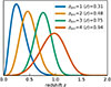 |
Fig. 1. Redshift bins used for this work, which were chosen to be generally representative of a Stage III survey. This figure is taken from Kacprzak & Fluri (2022). |
We followed the method introduced in Fluri et al. (2019) to calculate convergence κg maps. Using the PKDGRAV3 code (Potter et al. 2017), 57 unique cosmologies in the Ωm-σ8 plane were each simulated 12 times. Each simulation used 2563 particles in a volume of 5003 Mpc3, and the initial conditions were generated at a redshift of zinit = 50 using the MUSIC code (Hahn & Abel 2011). All simulations were run over 500 time steps, saving snapshots at intervals of Δz = 0.1 from z = 3.45 to z = 1.55 and Δz = 0.05 from z = 1.55 to z = 0. From the 3D simulated overdensity, δ3D, 2D convergence maps were projected using the UFALCON code (Sgier et al. 2019).
The convergence of a given pixel was calculated with the Born approximation:
![Mathematical equation: $$ \begin{aligned} \kappa \approx \sum _{b} W^{WL}_{b} \int _{\Delta z_b} \frac{dz}{E(z)} \, \delta _{3\mathrm{D}} [ \frac{c}{H_0} \mathcal{D} (z) \hat{n}^{pix},z] , \end{aligned} $$](/articles/aa/full_html/2026/05/aa53963-25/aa53963-25-eq3.gif) (1)
(1)
where 𝒟(z) is the dimensionless comoving distance, E(z) is defined by  , and
, and  is a unit vector pointing to the pixel. The sum ran over the redshift shells (that are Δzb in thickness), and the weight for each shell is defined as follows:
 (2)
(2)
The mean convergence of each map was subtracted:
 (3)
(3)
The maps were noised over with Gaussian noise:
![Mathematical equation: $$ \begin{aligned} \kappa _g = \text{ Normal}\left[ \kappa , \frac{\sigma _e}{\sqrt{n_{gal}}}\right] ,\end{aligned} $$](/articles/aa/full_html/2026/05/aa53963-25/aa53963-25-eq8.gif) (4)
(4)
where σe = 0.4 is the galaxy’s shape noise and ngal is the number of galaxies per pixel.
Because the simulations feature only dark matter, the physical modelling does not accurately describe the small scales where baryonic effects become apparent. The precise scale at which baryonic effects become significant is currently an active field of research, with results from hydrodynamical simulations varying depending on the implementation of galaxy formation physics (see e.g. Borrow et al. 2020; Ayromlou et al. 2023; Gebhardt et al. 2024). In this work, we chose to follow Porredon et al. (2022) and smooth the map at R = 4 Mpc/h to discard the smallest scales. Taking the pixel size into account, we applied the following additional Gaussian smoothing for the four redshift bins:
![Mathematical equation: $$ \begin{aligned} \sigma =[4.8,\ 3.5,\ 2.8,\ 2.5]\,\mathrm{arcmin}; \end{aligned} $$](/articles/aa/full_html/2026/05/aa53963-25/aa53963-25-eq9.gif) (5)
(5)
we did so to achieve the 4 Mpc/h smoothing. Each individual map obtained through this process is 5 × 5 degrees and 64 × 64 pixels. We constructed simulated 900 deg2 surveys by creating a mosaic of 6 × 6 maps. Noise was added on the fly for each realization during both training and prediction, and maps were randomly placed and flipped when creating the mosaic to avoid repetition. Smoothing was done before the mosaic was created to avoid blurring the edges between maps. Fig. 2 shows an example of a simulated survey.
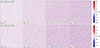 |
Fig. 2. Example of two simulated 900 deg2 surveys with four redshift bins, obtained by creating a mosaic of 6 × 6 individual 5 × 5 deg maps, with Gaussian noise and Gaussian smoothing on a R = 4 Mpc/h scale according to Eqs. (4) and (5). Even though the two surveys were obtained for very different cosmologies, the high noise level leads to little visual difference between the two. |
2.2. Neural networks
Most of the map analysis in this work was done using a convolutional neural network (CNN) that takes pixel maps as inputs and returns summary statistics corresponding to the cosmological parameters Ωm and σ8. The CNN is based on a ResNet architecture (He et al. 2015) and consists of four convolutional layers, ten residual layers with a kernel size of five, a stride of two, and the ReLu activation function. The last residual layer was flattened and fully connected to the output layer, which contains the summary statistics and their covariances. This architecture gives a total of ∼107 trainable parameters.
A power spectrum (PS) approach was also used, whereby we calculated the auto- and cross-spectra of the input maps and compressed the PS vectors into the same summary statistics as the CNN via a neural network. Conducting power spectrum analysis this way allowed for the simultaneous training of both networks and for the same likelihood analysis to be used on both CNN and PS outputs.
The power spectra of the κg maps were calculated by FFT and averaged in 20 logarithmically spaced ℓ bins over the ℓ ∈ [36, 4536] range. This gives a minimum interval of δℓ = 36, which is the resolution of the FFT. Calculating all auto- and cross-spectra over the four redshift bins gave ten spectra per simulated survey, which were then given as input to a network consisting of two fully connected layers with 1024 units and ReLu activation, and an output layer identical to that of the CNN predicting summary statistics and covariances. This gave ∼1.2 106 trainable parameters.
The training strategy for both network architectures uses a negative log-likelihood loss function for both network types:
 (6)
(6)
where θt is the true parameter vector, θp is the output summary vector, and Σp is the output covariance matrix. The networks were trained using stochastic gradient descent with the ADAM optimiser (Kingma & Ba 2017), with a batch size of 32 simulated surveys and a learning rate of 0.00005 for the CNN and 0.0025 for the PS neural network. We additionally applied gradient clipping using the method described in Seetharaman et al. (2020) using the 50th percentile. Both networks (including hyper-parameters) were taken directly from Kacprzak & Fluri (2022), created in TensorFlow (Abadi et al. 2016), and trained on the CSCS supercomputer Piz Daint using NVIDIA Tesla P100 16GB GPUs.
All models were trained for 100k batches, with very minimal improvement of the loss for the last 30k batches, which indicates reasonable convergence. We created a separate test set consisting of around 8% of the full dataset that was not used for training and calculated the loss for this set throughout training. No difference between training and testing loss appears for any model, indicating that over-fitting was not a problem, most likely due to the addition of noise at each realisation.
2.3. Likelihood analysis
The conditional probability distribution, p(θp|θt), was estimated by running a prediction through the trained networks with samples for all 57 combinations of (Ωm,σ8) from the simulation grid. p(θp|θt) was then modelled via a mixture density network (MDN) that uses a mixture of Gaussians at each θt to mimic the conditional probability distribution as closely as possible. The MDN predicts the means, covariances, and relative weights of its Gaussian components and is trained with stochastic gradient descent. The validation loss is monitored to prevent over-fitting, and we confirm that the MDN modelled the probability distribution correctly with four Gaussian components by directly comparing the two.
We then ran a Markov chain Monte Carlo (MCMC) analysis with the emcee algorithm (Foreman-Mackey et al. 2013) and the distribution given by the MDN. 200 chains of 128k samples were run for each model (or a single 1.28m chain to plot Fig. 5).
3. A novel approach to the interpretability problem
The unsimplified version of this network architecture presented in Kacprzak & Fluri (2022) shows the great potential that deep learning has to improve the analysis of weak-lensing surveys in the future, but it is hard to trust a ‘black-box’ analysis method whose limitations and potential biases are unknown, and we cannot optimise our future surveys for it if it became the main analysis method. It is therefore crucial to try to understand how the CNN works and where the information is coming from.
As more and more effort is put into developing deep-learning approaches to weak-lensing data analysis and great potential is starting to appear, ways to solve the interpretability problem are starting to be pursued. This work used a novel approach (at least in the field of weak-lensing): instead of using ‘a posteriori’ interpretability methods as in many studies where the network is first trained on the normal dataset and then analysed through various methods – such as sensitivity maps, which measure to what extent the output is affected by a variation of each input pixel (LeCun et al. 1998) – we chose to directly degrade the dataset and then train the networks with the modified data and see how much the constraining power is affected compared to a network trained with the full data. A similar approach was applied in the broader field of cosmology by, for example, Lucie-Smith et al. (2024) to help understand the importance of isotropic and anisotropic information when predicting halo masses from the initial density field. Villaescusa-Navarro et al. (2021b) also applied degradations to the training data to understand the impact on inference of a CNN trained to predict cosmological parameters from 2D-projected mass maps.
Because this approach requires re-training the networks for each degradation, it has the significant drawback of requiring a long computation time, which is why we used a simplified version of the pipeline presented in Kacprzak & Fluri (2022), but in return it allows for a very intuitive understanding of which parts of the surveys hold the most information for the network.
The architecture of the neural network is kept consistent throughout the study and was not optimized for each individual degradation. This choice was made to allow for a more direct comparison between degradations, but it means that the results presented here are specific to this architecture and could vary if the architecture were individually optimised for each case.
3.1. Data degradations
To degrade the data, we inserted layers in the neural network before the first convolutional layer that modified the data in a number of different ways. Smoothing scales are the only degradations for which the PS neural network was used. For all other degradations, only the CNN was used as it is the architecture of interest, the PS neural network simply being a way of implementing a PS analysis.
3.1.1. Smoothing scales
The first degradation was to change the scale at which the Gaussian smoothing of the maps is applied (see Sect. 2.1). Both the CNN and the PS neural network were trained after smoothing at each of the following scales:
![Mathematical equation: $$ \begin{aligned} R=[2,\ 4\ \mathrm{(reference)},\ 8,\ 16]\,\mathrm{Mpc/h} .\end{aligned} $$](/articles/aa/full_html/2026/05/aa53963-25/aa53963-25-eq11.gif) (7)
(7)
3.1.2. Starlet transform
Starlet transforms decompose a given image into i + 1 channels containing the details on a scale of ∼2i pixels for the first i channels and the remainder of the image for the last channel (see Starck et al. 2007 for a full description of starlet transforms). Summing all of the channels recovers the initial image. By performing starlet transforms of the maps, we were able to present the network with all of the information decomposed into multiple channels or select only certain scales. Fig. 3 shows an example of a convergence map separated into four channels containing different scales.
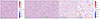 |
Fig. 3. Example of map separated into four channels by a starlet transform. Only the first redshift bin is shown, but all four were included in the training. The left panel is the initial map, and the rest are the four starlet transform channels. |
3.1.3. Convergence thresholds
Using thresholded ReLu layers, we separated the maps into three low-, mid-, and high-convergence regions. We chose the threshold to be κg = 0.014, which corresponds to a signal-to-noise ratio of 0.25. On average (this depends on cosmology and redshift), roughly 20% of the total pixels are in either the low or high regions and 60% are in the mid-convergence regions. Fig. 4 shows an example of a map separated into these three convergence regions. Pixels with κg values outside of the chosen range are set to a fixed value far outside the range. Different combinations of these regions, presented in the next section, are fed as input to the CNN.
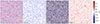 |
Fig. 4. Example of map separated into three convergence regions. Only the first redshift bin is shown, but all four were included in the training. From left to right we show the base map, the low-convergence regions, the mid-convergence regions, and finally the high-convergence regions. Pixels outside of the range appear in yellow for both high and low κ and in deep blue for mid κ. |
3.1.4. Fourier transform
By calculating the fast Fourier transform (FFT) of the maps, we provided the network with all of the information, but presented in Fourier space in the form of real and imaginary parts or amplitude and phase. We also studied limiting the information to just either the phase or amplitude.
3.1.5. Redshift shuffle and sum
We shuffled the data along the redshift axis, presenting simulated surveys with a random redshift order. We also summed all four redshift bins into a single map, removing all tomographic information from the survey.
3.1.6. Full pixel shuffling
We shuffled all the pixels from the four redshift bins to remove all spatial and redshift information. This essentially made the degraded maps equivalent to a histogram, while still keeping the network architecture identical.
3.2. Quantifying the network’s performance
The degradation layers were active during both training and prediction, meaning that the network never has access to the information that was removed. Therefore, if the constraints obtained were still comparable to the one obtained with the reference network (without degradation layers), we can assume that the network does not rely heavily on the removed information or at least that it is redundant and can be replaced in the inference process.
To measure the networks’ performances, we focused on two indicators: the standard deviation of the constraint on  , hereafter denoted σS8, and the information entropy of the MCMC chains. Information entropy is defined in Shannon (1948) as H = 𝔼[−log p(X)]. To calculate the entropy of an MCMC chain, which contains 128k samples that are [Ωm, σ8] pairs, we split the 2D prior space into 10k bins and created a histogram of the 128k samples. The entropy was then calculated as
![Mathematical equation: $$ \begin{aligned} H_{chain}= \ln \frac{1}{n_{bins}} - \left[ \, \sum _{b \in bins} \frac{f_{b}}{n_{samples}} \ln \frac{f_{b}}{n_{samples}} \right] , \end{aligned} $$](/articles/aa/full_html/2026/05/aa53963-25/aa53963-25-eq13.gif) (8)
(8)
where nbins = 10 k is the number of bins, nsamples = 128 k is the number of samples, and fb is the number of samples that lead to a prediction in the bin b.
Taking  as reference means that Hchain represents the loss of randomness compared to the prior. Having these two measurements allows for an objective quantification of information loss with each degradation, and both are defined in a smaller-is-better way for easy comparison.
We calculated both σS8 and Hchain for each MCMC chain and then calculated the mean and standard deviation of the two indicators for each model. Note that the means and standard deviations presented thereafter were obtained strictly on the post-processing and do not include any variability in the network-training phase. To include that variability, we would have needed to run multiple trainings for each degradation, which was impossible for computation time reasons.
4. Results
Figures 6–9 present the networks’ performances for all the data degradations studied in this work. We note that there is a great coherence between the two indicators: the order of the different degradations in σS8 and H is almost identical. The slight disagreements can be explained by one main difference between the two measurements: σS8 is not significantly affected by outliers when compared to the entropy, and it mostly probes how tight the central part of the distribution is.
For better visualisation of the difference in constraint tightness between the different degradations, Fig. 5 shows a comparison of the constraints obtained with no degradation (reference, in pink) and with only the low-convergence regions (low κ, in violet), a degradation that results in some of the worst performance observed in this work. The regions correspond to 68% and 95% confidence intervals.
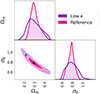 |
Fig. 5. Constraints on [Ωm, σ8] obtained by the CNN. The black dots mark the true value of parameters. |
4.1. Scales
Figure 6 presents all the results related to scales. We find that there is very good coherence between the performance when certain scales are removed via smoothing (top four rows) or through the removal of certain channels of the starlet transforms (bottom rows). The CNN seems very robust to the data being presented in one or multiple channels (this is further explored in Sect. 4.2).
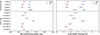 |
Fig. 6. Network performance for various scale-related degradations. Left panel shows σS8, which is the constraining power on S8; right panel shows H, which is the information entropy. The top four rows present the performance for various smoothing scales, for both the CNN and the PS neural network. The lower rows present the performance of the CNN for various scale ranges; this was achieved by keeping only certain starlet transform channels. |
From the results, we can deduce that the richest scales in terms of information are roughly from 8 to 12 Mpc/h; smoothing out smaller scales does not affect the constraining power, and only providing the network with smaller scales results in slightly worse performance. Interestingly, these scales correspond to the transition between linear and non-linear regimes at the considered redshifts, which could explain why they hold so much information. The fact that the smaller scales have comparatively little impact on the results is in contrast with the findings of Villaescusa-Navarro et al. (2021b), which showed that a CNN trained to predict cosmological parameters from 2D-projected mass maps was able to extract information down to very small scales (∼100 kpc/h). One key difference between that study and our analysis is that Villaescusa-Navarro et al. (2021b) used unprocessed mass maps from the CAMELS simulation suite (Villaescusa-Navarro et al. 2021a), which are of much higher resolution and smaller volumes than our simulated surveys, and they do not include any noise, whereas our simulated surveys include shape noise. To better disentangle data-intrinsic and noise-related effects, we studied the scale-related and convergence-threshold degradations without including shape noise (see Appendix A), and we found that the relative importance of small scales is higher in the absence of noise.
Keeping only very large scales of > 16 Mpc/h results in significantly worse performance than any other scale range with the CNN, but it only slightly degrades the PS neural network’s performance: this can be explained by the fact that non-Gaussian information (which the CNN has access to, but the PS does not) is contained on small, non-linear scales. An interesting feature to note is that removing the smallest (< 5 Mpc/h) and largest (> 20 Mpc/h) scales (second-to-last row in Fig. 6) seems to slightly improve the CNN’s performance, although not very significantly. This may be due to the fact that it allows the network to optimize its convolution kernels for the richest scales information-wise only and that part of the noise is removed.
4.2. Non-degrading transformations
Figure 7 presents all the results related to transformations that do not degrade the information, but present it in a different way. Starlet transforms in three or five channels do not cause any degradation of the CNN’s performance, and they may even improve it slightly, probably due to the fact that they are a form of data preparation allowing convolution kernels to be optimised specifically to extract information from a certain scale.
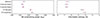 |
Fig. 7. CNN performance for various zero-loss transformations. Left panel shows σS8, which is the constraining power on S8; right panel shows H, which is the information entropy. The results for three or five channels starlet transform, as well as for a Fourier transform, in the form of either real and imaginary parts or amplitude and phase are presented. |
On the other hand, presenting the data in Fourier space, either as real and imaginary parts or amplitude and phase (as the CNN cannot handle data in the complex space) significantly degrades the network’s ability to extract information. While this is surprising given the fact that no information was removed, this highlights the fact that the CNN architecture is designed to work on real space images.
4.3. Convergence thresholds
Figure 8 presents all the results obtained when only keeping regions in certain convergence ranges (see Fig. 4 for an example of the input maps). We find that the mid-convergence regions hold the least information even though they represent the majority of the total area (60% of all pixels). This is consistent with what was concluded from Matilla et al. (2020) through different methods; pixels with extreme convergence values, i.e. peaks and voids, provide significantly more information to the CNN than the regions with intermediate convergence values. This is consistent with the findings of Lahiry et al. (2025), which studied the interpretability of a framework similar to that of Villaescusa-Navarro et al. (2021b). They found that their CNN extracted information from the most extreme over-dense and under-dense regions, with the peaks in the matter distribution containing the most information per pixel.
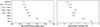 |
Fig. 8. CNN performance for various convergence regions’ selections. Left panel shows σS8, which is the constraining power on S8; right panel shows H, which is the information entropy. Low, mid, and high κ denote the low-, mid-, and high-convergence regions. The second row presents the performance of a network taking the high-convergence regions in one channel and the Fourier transform amplitude in another to mimic a summary statistics analysis method capable of extracting non-Gaussian information: the combination of the PS and peak counts or Minkowski functionals. |
Interestingly, even if they provide little information on their own, adding the mid-convergence regions back to either low- or high-convergence regions significantly improves the performance compared to low- or high-convergence regions alone. Combining the two extreme regions also improves the performance significantly. We can suppose that only one extreme region (especially high-convergence regions) mostly provides information on small, non-linear scales and lacks information on larger scales: Fig. 4 shows how the low- and high-convergence maps are essentially a collection of small, disconnected peaks and voids with a typical scale of ∼7 Mpc/h. Adding either the mid convergence (where connected regions are much larger) or the opposite extreme likely allows the network to access the information held on larger scales.
This hypothesis is also supported by the fact that combining the high-convergence regions (i.e. the peaks) with the Fourier transform amplitude, which only contains Gaussian information (like the larger scales), results in a performance that is essentially indistinguishable from the reference model with no data degradation. That result also suggests that the summary statistics approach of combining the power spectrum with peak count and/or Minkowski functionals (morphological descriptors containing information about the peaks) proposed by some studies (e.g. Pires et al. 2009; Dietrich & Hartlap 2010) can likely help reduce information loss.
4.4. Redshift and spatial information
Figure 9 presents all the results obtained when shuffling or summing along the redshift axis or shuffling all the pixels, removing spatial information altogether. Surprisingly, summing the redshift bins results in no significant performance degradation. This is likely due to the simple nature of this work: including astrophysical sources of uncertainty such as galaxy intrinsic alignment changes this result, as detailed in Appendix B. Interestingly, shuffling the redshift bins results in worse performance than summing them, even though there is theoretically at least as much information, showing that ill-presented data can lead to prediction errors by the network.
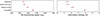 |
Fig. 9. CNN performance for redshift shuffling, redshift summing, and shuffling all pixels. Left panel shows σS8, which is the constraining power on S8; right panel shows H, which is the information entropy. |
Another surprising result is how removing all spatial information does not prevent the network from providing somewhat accurate predictions. The constraining power is comparable to that of the PS neural network, or to that of the CNN with access to the large scales only.
5. Discussion and conclusion
We built on a novel approach to weak-lensing-survey analysis through deep learning, via the use of convolutional neural networks, and investigated its behaviour to better understand the algorithm’s inference process. We started with a simplified version of the DeepLSS pipeline (Kacprzak & Fluri 2022), added pre-processing layers to the network to remove parts of the information contained in the dataset, and measured the constraining performance of the network for various degradations. In analysing how the performance varies, we tried to understand what parts and features of the surveys are most important in the network’s inference process.
Using the approach from Fluri et al. (2019, 2022), and Kacprzak & Fluri (2022), we ran N-body simulations of the Universe for various cosmological parameters’ values and used them to generate tomographic weak-lensing convergence κg maps via a pencil-beam approach. We created two networks to analyse the data: a residual convolutional neural network that takes the raw maps as input and a power spectrum neural network that first calculates all auto- and cross-spectra of the maps and then passes them through a simple neural network. Both architectures were trained using likelihood loss between outputs and true input parameters to compress the data into our two cosmological parameters of interest, Ωm and σ8, and their covariances. We then obtained constraints via Bayesian analysis with a MCMC sampler.
To understand the networks’ inference processes, we measured its performance with two indicators: σS8, which is the tightness of constraint on S8, and H, which is the information entropy of the posterior. We first set a reference by running the convolutional neural network on the unmodified dataset. We then introduced layers to the network to measure its performance on degraded data with some information removed. We removed certain scales, separated the data into low-, mid-, and high-convergence regions, and removed redshift or spatial information.
When including Stage-III-like shape noise, we find that the scales that seem to hold the most information are from 8 to 12 Mpc/h, which corresponds to the transition between linear and non-linear scales. As long as these scales are present in the data, the performance level is indistinguishable from that of the reference. Using only large scales (over 16 Mpc/h) leads to significantly worse performance, similarly to what we see for the power-spectrum approach. Using only smaller scales (below 10 Mpc/h) leads to slightly worse performance than what was seen in the reference case. We found that the relatively low importance of small scales in the inference process (in contrast to the finding of, e.g. Villaescusa-Navarro et al. 2021b) can be explained by the presence of shape noise that drowns out small-scale information (see Appendix A).
We report that separating the data into multiple channels via starlet transform does not affect performance, but presenting the data in Fourier space significantly reduces the constraining power.
We found that maps excluding extreme convergence regions (which we call mid-convergence) hold little information on their own compared to either low- or high-convergence regions (i.e. voids or peaks), but combining mid- with either low- or high-convergence regions significantly improved the performance compared to either extreme on its own. This is likely due to the fact that maps limited to either low- or high-convergence regions lack large connected regions and mainly contain non-Gaussian information. We also report that combining high convergence regions with the Fourier transform amplitude leads to the same performance as the reference run, confirming that combining power-spectrum and peak information (as suggested by, e.g. Pires et al. 2009 and Dietrich & Hartlap 2010) is a very good approach, and supporting our hypothesis that the lack of Gaussian information is impeding the network’s performance when provided with either only peaks or only voids.
Summing the redshift bins to create a non-tomographic survey surprisingly does not affect the performance significantly. We attribute this behaviour to our simplified baseline physical modelling, which lacks astrophysical uncertainties such as intrinsic alignment, because including intrinsic alignment changes these results (see Appendix B). Removing the spatial information altogether by shuffling the pixels leads to a significant performance loss, but the network is still able to make relevant predictions, with a performance similar to that of the power-spectrum approach.
Direct comparison with other studies is difficult due to the novelty of the field of interpretability of deep-learning methods applied to weak-lensing surveys and the diversity of methods used. We can nevertheless compare our results to the work of Matilla et al. (2020), the authors of which also tried to interpret the inference process of a CNN trained on weak-lensing data, albeit with a very different method. Using saliency maps to analyse the inference process of an already trained network, they found that the CNN relied heavily on the pixels with the most extreme values in the convergence maps, which is consistent with the results we present in Sect. 4.3. When studying noiseless maps, they found that pixels with the lowest convergence were most relevant to the decision, which does not agree with our findings. Nevertheless, when adding shape noise, as we did in this work, they found that the highest convergence regions were the most important in the network’s inference process, which aligns with our results. Saliency maps were also studied with the DeepLSS architecture in the original study (Kacprzak & Fluri 2022), but a direct comparison with this work is not straightforward as both convergence and galaxy density maps were used as combined probes in the original study, and the sensitivity study mainly indicated a correlation between the importance of pixels in one probe and their value in the other probe.
The key conclusion from this work is that, much like fixed summary statistics analysis methods, the performance of the convolutional neural network is strongest when provided with both Gaussian and non-Gaussian information, and that structures at the limit between linear and non-linear regimes are particularly important in its inference process. However, we note that this results from a combination of data-intrinsic and noise-related effects, as smaller scales also hold relevant information but are more affected by the presence of shape noise.
References
- Abadi, M., Agarwal, A., Barham, P., et al. 2016, arXiv e-prints [arXiv:1603.04467] [Google Scholar]
- Abbott, T. M. C., Aguena, M., Alarcon, A., et al. 2022, Phys. Rev. D, 105, 023520 [CrossRef] [Google Scholar]
- Aiola, S., Calabrese, E., Maurin, L., et al. 2020, JCAP, 2020, 047 [Google Scholar]
- Amon, A., Gruen, D., Troxel, M. A., et al. 2022, Phys. Rev. D, 105, 023514 [NASA ADS] [CrossRef] [Google Scholar]
- Ayromlou, M., Nelson, D., & Pillepich, A. 2023, MNRAS, 524, 5391 [CrossRef] [Google Scholar]
- Balkenhol, L., Dutcher, D., Mancini, A. S., et al. 2023, Phys. Rev. D, 108, 023510 [NASA ADS] [CrossRef] [Google Scholar]
- Bernardeau, F., Waerbeke, L. V., & Mellier, Y. 1997, A&A, 322, 1 [Google Scholar]
- Borrow, J., Anglés-Alcázar, D., & Davé, R. 2020, MNRAS, 491, 6102 [NASA ADS] [CrossRef] [Google Scholar]
- Bridle, S., & King, L. 2007, New J. Phys., 9, 444 [Google Scholar]
- Dietrich, J. P., & Hartlap, J. 2010, MNRAS, 402, 1049 [Google Scholar]
- Dvorkin, C., Mishra-Sharma, S., Nord, B., et al. 2022, arXiv e-prints [arXiv:2203.08056] [Google Scholar]
- Fluri, J., Kacprzak, T., Lucchi, A., et al. 2019, Phys. Rev. D, 100, 063514 [Google Scholar]
- Fluri, J., Kacprzak, T., Lucchi, A., et al. 2022, Phys. Rev. D, 105, 083518 [NASA ADS] [CrossRef] [Google Scholar]
- Foreman-Mackey, D., Hogg, D. W., Lang, D., & Goodman, J. 2013, PASP, 125, 306 [Google Scholar]
- Friedrich, O., Gruen, D., DeRose, J., et al. 2018, Phys. Rev. D, 98, 023508 [Google Scholar]
- Gebhardt, M., Anglés-Alcázar, D., Borrow, J., et al. 2024, MNRAS, 529, 4896 [NASA ADS] [CrossRef] [Google Scholar]
- Gong, Z., Halder, A., Barreira, A., Seitz, S., & Friedrich, O. 2023, JCAP, 2023, 040 [CrossRef] [Google Scholar]
- Gong, Z., Halder, A., Bohrdt, A., Seitz, S., & Gebauer, D. 2024, ApJ, 971, 156 [Google Scholar]
- Hahn, O., & Abel, T. 2011, MNRAS, 415, 2101 [Google Scholar]
- He, K., Zhang, X., Ren, S., & Sun, J. 2015, arXiv e-prints [arXiv:1512.03385] [Google Scholar]
- Heydenreich, S., Linke, L., Burger, P., & Schneider, P. 2023, A&A, 672, A44 [NASA ADS] [CrossRef] [EDP Sciences] [Google Scholar]
- Heymans, C., Tröster, T., Asgari, M., et al. 2021, A&A, 646, A140 [NASA ADS] [CrossRef] [EDP Sciences] [Google Scholar]
- Hirata, C. M., & Seljak, U. 2004, Phys. Rev. D, 70, 063526 [Google Scholar]
- Joachimi, B., Mandelbaum, R., Abdalla, F. B., & Bridle, S. L. 2011, A&A, 527, A26 [NASA ADS] [CrossRef] [EDP Sciences] [Google Scholar]
- Kacprzak, T., & Fluri, J. 2022, Phys. Rev. X, 12, 031029 [NASA ADS] [Google Scholar]
- Kingma, D. P., & Ba, J. 2017, arXiv e-prints [arXiv:1412.6980] [Google Scholar]
- Kirk, D., Rassat, A., Host, O., & Bridle, S. 2012, MNRAS, 424, 1647 [NASA ADS] [CrossRef] [Google Scholar]
- Lahiry, A., Bayer, A. E., & Villaescusa-Navarro, F. 2025, ApJ, 994, 129 [Google Scholar]
- LeCun, Y., Boser, B., Denker, J. S., et al. 1989, Neural Comput., 1, 541 [NASA ADS] [CrossRef] [Google Scholar]
- LeCun, Y., Bottou, L., Bengio, Y., & Ha, P. 1998, Proc. IEEE [Google Scholar]
- Lu, T., Haiman, Z., & Li, X. 2023, MNRAS, 521, 2050 [NASA ADS] [CrossRef] [Google Scholar]
- Lucie-Smith, L., Peiris, H. V., Pontzen, A., Nord, B., & Thiyagalingam, J. 2024, Phys. Rev. D, 109, 063524 [Google Scholar]
- Matilla, J. M. Z., Sharma, M., Hsu, D., & Haiman, Z. 2020, Phys. Rev. D, 102, 123506 [Google Scholar]
- Ocampo, I., Alestas, G., Nesseris, S., & Sapone, D. 2025, Phys. Rev. Lett., 134, 041002 [Google Scholar]
- Pan, S., Liu, M., Forero-Romero, J., et al. 2020, Sci. China Phys. Mech. Astron., 63, 110412 [NASA ADS] [CrossRef] [Google Scholar]
- Piras, D., & Lombriser, L. 2024, Phys. Rev. D, 110, 023514 [Google Scholar]
- Pires, S., Starck, J. L., Amara, A., Réfrégier, A., & Teyssier, R. 2009, A&A, 505, 969 [NASA ADS] [CrossRef] [EDP Sciences] [Google Scholar]
- Planck Collaboration XVI. 2014, A&A, 571, A16 [NASA ADS] [CrossRef] [EDP Sciences] [Google Scholar]
- Planck Collaboration VI. 2020, A&A, 641, A6 [NASA ADS] [CrossRef] [EDP Sciences] [Google Scholar]
- Porredon, A., Crocce, M., Elvin-Poole, J., et al. 2022, Phys. Rev. D, 106, 103530 [NASA ADS] [CrossRef] [Google Scholar]
- Potter, D., Stadel, J., & Teyssier, R. 2017, Comput. Astrophys., 4, 2 [NASA ADS] [CrossRef] [Google Scholar]
- Ravanbakhsh, S., Oliva, J., Fromenteau, S., et al. 2016, in Proc. of the 33rd International Conference on International Conference on Machine Learning – Volume 48, ICML’16 (New York, NY, USA: JMLR.org), 2407 [Google Scholar]
- Refregier, A. 2003, ARA&A, 41, 645 [NASA ADS] [CrossRef] [Google Scholar]
- Riess, A. G., Yuan, W., Macri, L. M., et al. 2022, ApJ, 934, L7 [NASA ADS] [CrossRef] [Google Scholar]
- Samek, W., Montavon, G., Lapuschkin, S., Anders, C. J., & Müller, K.-R. 2021, Proc. IEEE, 109, 247 [Google Scholar]
- Seetharaman, P., Wichern, G., Pardo, B., & Roux, J. L. 2020, arXiv e-prints [arXiv:2007.14469] [Google Scholar]
- Sgier, R., Réfrégier, A., Amara, A., & Nicola, A. 2019, JCAP, 2019, 044 [Google Scholar]
- Shannon, C. E. 1948, BSTJ, 27, 379 [Google Scholar]
- Starck, J.-L., Fadili, J., & Murtagh, F. 2007, IEEE Trans. Image Process., 16, 297 [Google Scholar]
- Takada, M., & Jain, B. 2003a, MNRAS, 340, 580 [NASA ADS] [CrossRef] [Google Scholar]
- Takada, M., & Jain, B. 2003b, MNRAS, 344, 857 [Google Scholar]
- Villaescusa-Navarro, F., Anglés-Alcázar, D., Genel, S., et al. 2021a, ApJ, 915, 71 [NASA ADS] [CrossRef] [Google Scholar]
- Villaescusa-Navarro, F., Genel, S., Angles-Alcazar, D., et al. 2021b, arXiv e-prints [arXiv:2109.10360] [Google Scholar]
- Villaescusa-Navarro, F., Wandelt, B. D., Anglés-Alcázar, D., et al. 2022, ApJ, 928, 44 [NASA ADS] [CrossRef] [Google Scholar]
- Villanueva-Domingo, P., & Villaescusa-Navarro, F. 2021, ApJ, 907, 44 [Google Scholar]
- Wright, A. H., Stölzner, B., Asgari, M., et al. 2025, A&A, 703, A158 [NASA ADS] [CrossRef] [EDP Sciences] [Google Scholar]
- Zürcher, D., Fluri, J., Sgier, R., et al. 2022, MNRAS, 511, 2075 [CrossRef] [Google Scholar]
Appendix A: Results without shape noise
In this Appendix, we present the results obtained when galaxy shape noise was not included. As it is the only source of noise in our simplified modelling, this means that the input data used in this part of the study was fully noiseless. While this is not realistic, this allows us to separate actual data-intrinsic effects from effects due to the presence of noise, which will vary depending on the specific modelling of the noise (e.g., when trying to mimic a Stage-IV weak-lensing survey, instead of the Stage-III-like surveys we study). We replicate our study of the scale-related and convergence threshold degradations, with the only changes being the absence of noise.
The results of the scale-related degradations (i.e. varying the smoothing scale and selecting various starlet decomposition channels) are presented in Fig. A.1. The results of the convergence threshold degradations are presented in Fig A.2. The first notable difference with the main analysis is that while the general agreement is reasonable, there is less consistency between the two indicators of constraining power. To draw our conclusions, we choose to focus on the information entropy H, which is more sensitive to outliers and thus better probes the full posterior distribution.
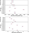 |
Fig. A.1. CNN performance for various scale related degradations, when excluding shape noise. Top panel is σS8, the constraining power on S8, bottom panel is H, the information entropy. The top four rows present the performance for various smoothing scales. The lower rows present the performance of the CNN for various scale range, obtained by keeping only certain starlet transform channels. |
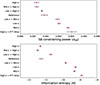 |
Fig. A.2. CNN performance for various convergence regions selections, when excluding shape noise. Top panel is σS8, the constraining power on S8, bottom panel is H, the information entropy. Low/mid/high κ denotes the low/mid/high convergence regions. The second row presents the performance of a network taking as input the high convergence regions in one channel and the Fourier transform amplitude in another, to mimic a summary statistics analysis method capable of extracting non-Gaussian information: the combination of the PS and peak counts/Minkowski functionals. |
The first conclusion from the scale-related degradations is that the network is able to extract information down to the smallest scales, as shown by the fact that the performance consistently improves when the smoothing scale is decreased. This is in contrast with the main analysis where small scales have a smaller impact on constraining power, likely due to the presence of shape noise dominating these scales. Villaescusa-Navarro et al. (2021b) found similar results when studying the impact of smoothing scales on the constraining power of a CNN trained on noiseless 2D matter density maps, showing that the network was able to extract information down to the smallest scales available.
One interesting result is that keeping only the scales below 10 Mpc/h actually improves the performance compared to the reference case. This suggests that in the absence of noise, small scales contain a lot of information that can compensate for the lack of larger scale information. It is challenging to explain how removing information leads to better performance, but it might stem from the fact that it allows the network to optimize its convolution kernels for the most relevant scales. Overall, the conclusion of the scale-related degradations is that, in the noiseless case, the network is able to extract information from all scales, including the smallest ones, and that small scales (≲10 Mpc/h) seem particularly important in the inference process.
There are two main differences with the main analysis when studying the convergence region selections in the noiseless case. First, the peaks seem to be even more important in the inference process, with the best constraining power being obtained when they are included. However, we find that in this context, the combination of high convergence regions with the FFT amplitude leads to a very degraded performance, unlike in the main study. This is quite surprising, since the network is able to reach the reference constraining power with only the high convergence regions. Even if it didn’t bring any information, setting the weights of the FFT amplitude channel to zero should have allowed for precise inference.
Appendix B: Results including intrinsic alignment
In this Appendix, we present the results obtained when modelling galaxy intrinsic alignment in the convergence maps. Intrinsic alignment is a source of systematic error in weak lensing surveys that arises from the fact that galaxies are not randomly orientated in the Universe, but could be aligned with each other due to large-scale tidal fields. This leads to a correlation between the shapes of galaxies and the weak lensing signal, which can be a significant source of bias in the analysis of weak lensing surveys (Hirata & Seljak 2004). Additionally, the magnitude of this effect depends on the physics of galaxy formation, and is very difficult to estimate from either simulations or theoretical calculations. Given the fact that the aim of this work is not to provide constraints or even to forecast constraining power, we chose to present the main analysis without including this effect, and verify here whether any conclusions are changed with its inclusion.
To model intrinsic alignment we follow the method used in Kacprzak & Fluri (2022) (originally derived from Zürcher et al. 2022), based on a non-linear alignment model (Bridle & King 2007; Joachimi et al. 2011). We create intrinsic alignment κIA maps for each redshift bin following Eq.1 in a similar way to the convergence maps, except that the kernel is the intrinsic alignment kernel, given by:
 (B.1)
(B.1)
where n(z) is the redshift distribution of galaxies in a given redshift bin, zs and z0 are the source and observer redshifts, and F(z) is a cosmology-dependent term:
 (B.2)
(B.2)
where C1 = 5.10−14h−2 M⊙ Mpc3, ρcrit is the critical density of the Universe, and D+(z) is the linear growth factor (normalized to D+(0) = 1). Finally, the mean of each intrinsic alignment map is removed.
The intrinsic alignment maps are then added to the convergence maps on the fly during the training and prediction process, using a single effective scaling value per redshift bin i:
 (B.3)
(B.3)
with
 (B.4)
(B.4)
where ni(z) is the redshift distribution of galaxies in the redshift bin i, AIA is the intrinsic alignment amplitude, and ηAIA is the intrinsic alignment redshift evolution. When intrinsic alignment is included, AIA and ηAIA are treated as parameters of the global model, and are varied during training and predicted by the network along with Ωm and σ8 during the prediction step. Large flat priors are used for both parameters ([ − 6, 6] for AIA and [ − 4, 6] for ηAIA).
Fig.B.1 to B.4 present the networks’ performance for all the data degradations studied in this work, but with the addition of intrinsic alignment. We find that the results are in general agreement with those obtained without intrinsic alignment, with an overall worse constraining power and less difference between the different degradations. The small scales seem less important in this case, with the constraining power not diminishing as much as in the baseline analysis when the smoothing scale is increased. The other significant difference is that the performance of the network when summing the redshift bins is now significantly worse than that of the reference model. This is likely due to the fact that the network is unable to correctly fit for intrinsic alignment without redshift information, as the evolution of intrinsic alignment with redshift is one of its potential distinguishing features from cosmic shear.
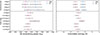 |
Fig. B.1. Network performance for various scale related degradations, when including intrinsic alignment. Left panel is σS8, the constraining power on S8, right panel is H, the information entropy. The top four rows present the performance for various smoothing scales, for both CNN and PS neural network. The lower rows present the performance of the CNN for various scale range, obtained by keeping only certain starlet transform channels. |
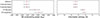 |
Fig. B.2. CNN performance for various zero-loss transformations, when including intrinsic alignment. Left panel is σS8, the constraining power on S8, right panel is H, the information entropy. The results for 3 or 5 channels starlet transform as well as for a Fourier transform in the form of either real and imaginary parts or amplitude and phase are presented. |
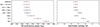 |
Fig. B.3. CNN performance for various convergence regions selections, when including intrinsic alignment. Left panel is σS8, the constraining power on S8, right panel is H, the information entropy. Low/mid/high κ denotes the low/mid/high convergence regions. The second row presents the performance of a network taking as input the high convergence regions in one channel and the Fourier transform amplitude in another, to mimic a summary statistics analysis method capable of extracting non-Gaussian information: the combination of the PS and peak counts/Minkowski functionals. |
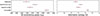 |
Fig. B.4. CNN performance for redshift shuffling, redshift summing and shuffling all pixels, when including intrinsic alignment. Left panel is σS8, the constraining power on S8, right panel is H, the information entropy. |
All Figures
|
Fig. 1. Redshift bins used for this work, which were chosen to be generally representative of a Stage III survey. This figure is taken from Kacprzak & Fluri (2022). |
| In the text | |
|
Fig. 2. Example of two simulated 900 deg2 surveys with four redshift bins, obtained by creating a mosaic of 6 × 6 individual 5 × 5 deg maps, with Gaussian noise and Gaussian smoothing on a R = 4 Mpc/h scale according to Eqs. (4) and (5). Even though the two surveys were obtained for very different cosmologies, the high noise level leads to little visual difference between the two. |
| In the text | |
|
Fig. 3. Example of map separated into four channels by a starlet transform. Only the first redshift bin is shown, but all four were included in the training. The left panel is the initial map, and the rest are the four starlet transform channels. |
| In the text | |
|
Fig. 4. Example of map separated into three convergence regions. Only the first redshift bin is shown, but all four were included in the training. From left to right we show the base map, the low-convergence regions, the mid-convergence regions, and finally the high-convergence regions. Pixels outside of the range appear in yellow for both high and low κ and in deep blue for mid κ. |
| In the text | |
|
Fig. 5. Constraints on [Ωm, σ8] obtained by the CNN. The black dots mark the true value of parameters. |
| In the text | |
|
Fig. 6. Network performance for various scale-related degradations. Left panel shows σS8, which is the constraining power on S8; right panel shows H, which is the information entropy. The top four rows present the performance for various smoothing scales, for both the CNN and the PS neural network. The lower rows present the performance of the CNN for various scale ranges; this was achieved by keeping only certain starlet transform channels. |
| In the text | |
|
Fig. 7. CNN performance for various zero-loss transformations. Left panel shows σS8, which is the constraining power on S8; right panel shows H, which is the information entropy. The results for three or five channels starlet transform, as well as for a Fourier transform, in the form of either real and imaginary parts or amplitude and phase are presented. |
| In the text | |
|
Fig. 8. CNN performance for various convergence regions’ selections. Left panel shows σS8, which is the constraining power on S8; right panel shows H, which is the information entropy. Low, mid, and high κ denote the low-, mid-, and high-convergence regions. The second row presents the performance of a network taking the high-convergence regions in one channel and the Fourier transform amplitude in another to mimic a summary statistics analysis method capable of extracting non-Gaussian information: the combination of the PS and peak counts or Minkowski functionals. |
| In the text | |
|
Fig. 9. CNN performance for redshift shuffling, redshift summing, and shuffling all pixels. Left panel shows σS8, which is the constraining power on S8; right panel shows H, which is the information entropy. |
| In the text | |
|
Fig. A.1. CNN performance for various scale related degradations, when excluding shape noise. Top panel is σS8, the constraining power on S8, bottom panel is H, the information entropy. The top four rows present the performance for various smoothing scales. The lower rows present the performance of the CNN for various scale range, obtained by keeping only certain starlet transform channels. |
| In the text | |
|
Fig. A.2. CNN performance for various convergence regions selections, when excluding shape noise. Top panel is σS8, the constraining power on S8, bottom panel is H, the information entropy. Low/mid/high κ denotes the low/mid/high convergence regions. The second row presents the performance of a network taking as input the high convergence regions in one channel and the Fourier transform amplitude in another, to mimic a summary statistics analysis method capable of extracting non-Gaussian information: the combination of the PS and peak counts/Minkowski functionals. |
| In the text | |
|
Fig. B.1. Network performance for various scale related degradations, when including intrinsic alignment. Left panel is σS8, the constraining power on S8, right panel is H, the information entropy. The top four rows present the performance for various smoothing scales, for both CNN and PS neural network. The lower rows present the performance of the CNN for various scale range, obtained by keeping only certain starlet transform channels. |
| In the text | |
|
Fig. B.2. CNN performance for various zero-loss transformations, when including intrinsic alignment. Left panel is σS8, the constraining power on S8, right panel is H, the information entropy. The results for 3 or 5 channels starlet transform as well as for a Fourier transform in the form of either real and imaginary parts or amplitude and phase are presented. |
| In the text | |
|
Fig. B.3. CNN performance for various convergence regions selections, when including intrinsic alignment. Left panel is σS8, the constraining power on S8, right panel is H, the information entropy. Low/mid/high κ denotes the low/mid/high convergence regions. The second row presents the performance of a network taking as input the high convergence regions in one channel and the Fourier transform amplitude in another, to mimic a summary statistics analysis method capable of extracting non-Gaussian information: the combination of the PS and peak counts/Minkowski functionals. |
| In the text | |
|
Fig. B.4. CNN performance for redshift shuffling, redshift summing and shuffling all pixels, when including intrinsic alignment. Left panel is σS8, the constraining power on S8, right panel is H, the information entropy. |
| In the text | |
Current usage metrics show cumulative count of Article Views (full-text article views including HTML views, PDF and ePub downloads, according to the available data) and Abstracts Views on Vision4Press platform.
Data correspond to usage on the plateform after 2015. The current usage metrics is available 48-96 hours after online publication and is updated daily on week days.
Initial download of the metrics may take a while.