| Issue |
A&A
Volume 695, March 2025
|
|
|---|---|---|
| Article Number | A132 | |
| Number of page(s) | 15 | |
| Section | Interstellar and circumstellar matter | |
| DOI | https://doi.org/10.1051/0004-6361/202553698 | |
| Published online | 14 March 2025 | |
Guidelines for non-LTE modelling of cyanopolyynes
1
Univ Rennes, CNRS, IPR (Institut de Physique de Rennes) –
UMR 6251,
35000
Rennes, France
2
Nantes Université, CNRS, CEISAM,
UMR 6230,
44000
Nantes, France
★ Corresponding author; This email address is being protected from spambots. You need JavaScript enabled to view it.
Received:
7
January
2025
Accepted:
10
February
2025
Abstract
Cyanopolyynes are abundant and widespread in cold molecular clouds. Their abundances are typically determined under the assumption of local thermodynamic equilibrium (LTE) or through non-LTE analysis based on approximate collisional rate coefficients. Here, we present the first quantum mechanical scattering data for HC5N and HC7N in collisions with helium. We used both close-coupling (CC) and coupled-states (CS) methods to compute excitation cross-sections. We then derived rate coefficients for the first energy levels of HC5N and HC7N. A comparative analysis between the CC and CS results reveals an agreement better than a factor of two for high-magnitude rate coefficients. However, we found that the derivation of approximate HC5N and HC7N rate coefficients from those of HCN and HC3N using a size proportionality relationship, as has been previously done in the literature, leads to an overestimation of the collisional data by up to two orders of magnitude. To assess the sensitivity of cyanopolyyne line intensities to collisional rate coefficients, we compared LTE predictions with various non-LTE models using different rate coefficients. Under the typical physical conditions of cold molecular clouds, the LTE assumption and radiative transfer calculations based on approximate collisional rate coefficients strongly overestimate high-frequency line intensities, while the non-LTE models based on the HC3N collisional rate coefficients as a proxy for HC5N and HC7N remain accurate within 10%. We therefore recommend revisiting the abundance estimates for HC5N and HC7N using the new rate coefficients. For HC9N and HC11N, adopting HC7N collisional data in line modelling is expected to be highly accurate.
Key words: molecular data / molecular processes / radiative transfer / scattering / ISM: abundances / ISM: molecules
© The Authors 2025
 Open Access article, published by EDP Sciences, under the terms of the Creative Commons Attribution License (https://creativecommons.org/licenses/by/4.0), which permits unrestricted use, distribution, and reproduction in any medium, provided the original work is properly cited.
This article is published in open access under the Subscribe to Open model. This email address is being protected from spambots. You need JavaScript enabled to view it. to support open access publication.
1 Introduction
Cyanopolyynes, a particularly interesting family of carbon-chain molecules, are characterized by a linear back-bone that features a hydrogen atom at one end and a cyanide (CN) group at the other. They are ubiquitous in the interstellar medium (ISM) and have been observed throughout various stages of star formation, ranging from dark clouds to protoplanetary disks (Walmsley et al. 1980; Chapillon et al. 2012). Some of these molecules, for example HC2n+1N (n = 1–4), have large column densities that vary from 1012 cm−2 up to a few 1014 cm−2 in L1544, TMC-1, and asymptotic giant branch (AGB) stars such as CRL 2688 and IRC+10216 (Bianchi et al. 2023; Loomis et al. 2016; Pardo et al. 2020).
The cyanopolyynes observed towards TMC-1 exhibit a decreasing linear relationship between the log of their column density and size (Loomis et al. 2016). This pattern can be attributed to a formation mechanism governed by a few gas-phase chemical reactions that extend the carbon chain (Fukuzawa et al. 1998). Observations towards CRL 2688 and IRC+10216 also reveal that the abundances of cyanopolyynes follow a similar trend, which indicates that the gas-phase formation mechanisms are likely to be analogous in both cold cores and AGB stars (Truong et al. 1993). Based on this linear pattern and the assumption of a quite simple chemistry, both observational and laboratory studies have aimed at identifying larger cyanopolyynes. This effort led to the discovery of HC11N in TMC-1 (Bell et al. 1997), a finding that was subject to debate until the observations of Loomis et al. (2021). The estimation of the HC11N column density, the largest interstellar cyanopolyyne detected to date, was found to be much lower than what could have been predicted from the log-linear trend (Loomis et al. 2016) derived from column densities of smaller cyanopolyynes.
Loomis et al. (2021) reevaluated the column densities of cyonopolyynes detected towards TMC-1 using a significantly more comprehensive set of observational data than in their previous work (Loomis et al. 2016). The updated column densities obey the same decreasing log-linear trend, but with a weaker slope in absolute value. Indeed, the column density remains unchanged for n = 1 , but progressively increases with respect to the previous results as n grows. The maximum increase was seen for HC11N, which enabled its column density to be well reproduced by an extrapolation of the log-linear trend derived from the column density of the other cyanopolyynes. For the L1544 prestellar core, Bianchi et al. (2023) observed a similar pattern but with lower column densities with respect to TMC-1, which suggests that the same chemistry governs the formation and destruction mechanisms of cyanopolyynes in both sources.
However, one should keep in mind that the column densities of larger cyanopolyynes, from HC5N to HC11N, have been derived under the assumption of local thermodynamic equilibrium (LTE; Bell et al. 1997, 1998; Loomis et al. 2016, 2021). The latter authors estimated critical densities ranging from 3 × 102 cm−3 to 9 × 102 cm−3 by scaling the collisional rate coefficients of HC3N (Green & Chapman 1978) following the size dependency rule as suggested by Snell et al. (1981). These small values with respect to the gas density in TMC-1, ~104 cm−3, allowed the authors to assume fully thermalized lines. However, they stated that future studies on collisional rate coefficients of larger cyanopolyynes are required to shed light on the statistical equilibrium calculations. Indeed, the critical densities were calculated using a simplified formula that does not reflect the full complexity of radiative transfer processes. In addition, the calculations relied on roughly estimated collisional rate coefficients.
Given the importance of performing actual radiative transfer calculations to determine accurate molecular abundances, Al-Edhari et al. (2017) and Bianchi et al. (2023) used a non-LTE model, based on approximate collision rate coefficients. In practice, they updated the size dependency rule of Snell et al. (1981), since they considered that it does not scale proportionally across all transitions and derived rate coefficients for HC5N and HC7N induced by collisions with H2 from the scattering data of HCN-H2 and HC3N-H2 (Ben Abdallah et al. 2012; Wernli et al. 2007). However, the authors encourage investigation of the collisional excitation of these cyanopolyynes using state-of-the-art computational methods, as the uncertainty of their calculations has not been quantified.
To the best of our knowledge, among the members of the cyanopolyynes family, only the scattering of HC3N have been properly studied. The first set of rate coefficients for HC3N were provided by Green & Chapman (1978) for temperatures up to 100 K, using He as a projectile. These authors used quasi-classical trajectory in their scattering calculations. To satisfy the precision required when modelling astronomical lines, Wernli et al. (2007) used a state-of-the-art quantum mechanical approach to revisit the excitation of HC3N induced by collisions with He. In cold interstellar clouds where cyanopolyynes have been observed, H2 is the most abundant colliding partner. Therefore, Wernli et al. (2007) also investigated the excitation of HC3N by both para- and ortho-H2 at low temperature. The analysis of their results led to two main conclusions; (i) the scattering of HC3N is slightly sensitive to the ortho and para forms of H2 and (ii) the rate coefficients of HC3N induced by collisions with He can be scaled up to roughly estimate those due to para-H2 impact. Following this approach, in this work we investigate the collisions of HC5N and HC7N with He at low temperature, as He is a reasonable template for H2 in the case of cyanopolyynes. Furthermore, we revisit the scattering of HC3N by He, extending the rotational basis to generate a more comprehensive dataset, since Wernli et al. (2007) were limited to the 11 low-lying energy levels.
The structure of this paper is as follows: Section 2 provides a detailed description of the scattering calculations. Section 3 estimates the impact of the new rate coefficients on astronomical modelling and Sect. 4 presents the concluding remarks.
2 Scattering calculations
The potential energy surfaces (PESs) that describe the interaction between HC2n+ıN (n = 1,2,3) and He were constructed using the Jacobi coordinate system, with the targets considered as rigid rotors (Bop & Lique 2024). The PESs were calculated at the highly accurate CCSD(T)-F121/aug-cc-pVTZ2 level of theory (Knizia et al. 2009; Dunning Jr 1989), as implemented in the MOLPRO quantum chemistry package (Werner et al. 2015). To capture the interaction across all possible geometries, the Radial Angular Network with Gradual Expansion (RANGE) approach was employed, which ensures an effective analytical representation of the PESs. For more details on this method and the construction of the PESs, we refer the readers to Bop & Lique (2024).
Spectroscopic constants in cm−1.
2.1 Cross-sections
We implemented the PESs mentioned above in the MOLSCAT computer code using the VSTAR procedure (Hutson & Green 1994). We derived the long-range interaction potentials by extrapolating the radial coefficients using the following inverse power law:
 (1)
(1)
The parameters Cl and ηl were determined using the three last distances to ensure a smooth decay of the potentials.
We investigated state-to-state inelastic scattering processes of HC2n+1 N by He, and we only considered the rotational excitation and de-excitation as follows:
 (2)
(2)
where j stands for the rotational quantum number of the cyanopolyynes. We computed the energy levels of the cyanopolyynes using the rotational and centrifugal distortion spectroscopic constants B0 and D0, as indicated in Table 1 (Thorwirth et al. 2000; Alexander et al. 1976; McCarthy et al. 2000).
Figure 1 shows the structure of the rotational manifolds for the three cyanopolyynes for internal energies below 30 cm−1. The number of energy levels increases with the size of the HC2n+1N molecules. The rotational constant, which governs the internal energy structure, is inversely proportional to the mass and the length of the cyanopolyynes. We note that the number of channels3 involved in the scattering calculations increases with the increase in the size of the rotational basis. Therefore, employing exact quantum mechanical calculations becomes very demanding for longer cyanopolyynes, such as HC5N and HC7N, as the central processing unit (CPU) time is proportional to the cube of the number of channels.
To overcome such a limitation, we only used the ‘exact’ close-coupling (CC) quantum mechanical approach (Alexander 1977) for transitions involving internal energies below 30 cm−1, that is, the 26 and 40 low-lying rotational levels of HC5N and HC7N, respectively. For high-lying rotational levels, which have internal energies up to 100 cm−1, we used the coupled-states (CS) quantum mechanical approximation (McGuire & Kouri 1974). To estimate the accuracy of the CS method, in the case of HC3N, which has a reasonable number of rotational levels below 100 cm−1, we employed both the CC and CS approaches to generate two sets of cross-sections for the same energy range. All numerical integrations were performed using the log derivative-airy propagator (Alexander & Manolopoulos 1987).
To converge cross-sections that involve energy levels below 30 cm−1, we included several channels above this rotational threshold by allowing j to vary up to jmax, as shown in Table 2. We determined additional parameters, such as the integration boundaries and the step size, to ensure sub-percent convergence of the cross-sections. To enable a smooth description of the resonances, the total energy (E) range was spanned up to 30 cm−1 with a fine step size of 0.1 cm−1, 0.05 cm−1, and 0.01 cm−1 for HC3N, HC5N, and HC7N, respectively. Using small step sizes, typically on the same order of magnitude as the rotational constants of the cyanopolyynes, ensures accurate resonance descriptions, particularly for energies just above the rotational threshold. Between 30 cm−1 and 100 cm−1, the total energies were equally spaced by 0.1 cm−1. For 100 cm−1 ≤ E ≤ 400 cm−1, the step was smoothly increased up to 10 cm−1 except for the CC calculations of HC5N and HC7N. In the latter cases, the total energies were spanned up to E = 100 cm−1.
Figure 2 illustrates the dependence of the cross-sections on kinetic energy (Ek). Apart from resonances, cross-sections calculated using both CC and CS levels of theory exhibit similar behaviour. Compared to CC results, the CS results display more pronounced Feshbach and shape resonances, especially for the 1 → 0 transition. This probably arises from limitations in the CS approximation.
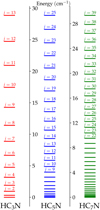 |
Fig. 1 Low-lying rotational energy levels of HC2n+ıN (n = 1, 2, 3) considered in this work. |
Size of the rotational basis (jmax).
2.2 Rate coefficients
By means of thermal averaging over the Maxwell-Boltzmann kinetic energy distribution of the calculated cross-sections, we derived rate coefficients (k) for the HC2n+1N-He collisional systems as follows:
 (3)
(3)
where µ is the reduced mass (in atomic units) of HC2n+1N-He collisional systems, and β is defined as the inverse of the Boltzmann constant multiplied by the temperature. For HC5N and HC7N, we derived collisional rate coefficients for kinetic temperatures up to 15 K and 50 K using the CC and CS cross-sections, respectively. In the case of HC3N, we computed two collisional datasets, that is, CC and CS base rate coefficients, up to 50 K. However, all comparisons made in this section are limited to 10 K, which is the typical gas kinetic temperature of cold molecular clouds, that is, the media where cyanopolyynes have been observed.
In Fig. 3, we evaluate the accuracy of CS-derived rate coefficients against CC scattering data for HC3N, HC5N, and HC7N. Overall, the CS approximation overestimates the scattering data compared to the ‘exact’ CC method by up to a factor of two for the high-magnitude rate coefficients. For the low-magnitude rate coefficients, significant deviations are observed for the three cyanopolyynes. However, these data are expected to play only a minor role in radiative transfer calculations. We can then conclude that the CS approach is reasonably accurate for providing collisional data for cyanopolyynes.
In Fig. 4, we compare the rate coefficients of HCN (Dumouchel et al. 2010), HC3N, HC5N, and HC7N induced by collisions with He at 10 K. As previously reported for HCN and HC3N (Ben Abdallah et al. 2012; Wernli et al. 2007), we observe a similar propensity rule for the longer cyanopolyynes, specifically the dominance of even Δj transitions. Changing the initial rotational level from j = 10 to 18 and 25, as shown in the right-hand and lower panels, confirms that Δj = 2 transitions consistently emerge as the most prominent. The novelty of this plot lies in its comparative analysis of rate coefficients across the four molecules. Generally, the excitation behaviour for these species is quite similar for low Δ j transitions, especially for even values. However, the rate coefficients for HCN decrease rapidly beyond Δj > 5, while those for HC3N and HC5N begin to drop at larger Δj values.
We assessed the validity of the approximate collisional rate coefficients first proposed by Al-Edhari et al. (2017) and recently used by Bianchi et al. (2023). These authors revised the size proportionality rule introduced by Snell et al. (1981), and incorporated the dependency of collisional rate coefficients on molecular transitions. The original method of Snell et al. (1981) was based on the classical collision theory principle that the impact parameter increases with the molecular size. However, Al-Edhari et al. (2017) and Bianchi et al. (2023) observed that this scaling is not proportional for all transitions and subsequently refined the approximation of Snell et al. (1981) as follows:
![Mathematical equation: $k_{j \to j'}^{{\rm{H}}{{\rm{C}}_7}{\rm{N}} - {\rm{He}}}(T) = k_{j \to j'}^{{\rm{H}}{{\rm{C}}_3}{\rm{N}} - {\rm{He}}}(T)\left[ {{{k_{j \to j'}^{{\rm{H}}{{\rm{C}}_3}{\rm{N}} - {\rm{He}}}(T)} \over {k_{j \to j'}^{{\rm{HCNe}}}(T)}}} \right]$](/articles/aa/full_html/2025/03/aa53698-25/aa53698-25-eq4.png) (4)
(4)
![Mathematical equation: $k_{j \to j'}^{{\rm{H}}{{\rm{C}}_5}{\rm{N}} - {\rm{H}}{{\rm{e}}^2}}(T) = {1 \over 2}\left[ {k_{j \to j'}^{{\rm{H}}{{\rm{C}}_3}{\rm{N}} - {\rm{H}}{{\rm{e}}^2}}(T) + k_{j \to j'}^{{\rm{H}}{{\rm{C}}_7}{\rm{N}} - {\rm{H}}{{\rm{e}}^2}}(T)} \right].$](/articles/aa/full_html/2025/03/aa53698-25/aa53698-25-eq5.png) (5)
(5)
Hereafter, we refer to this approximation as the ‘extrapolation’ method.
In the left-hand panel of Fig. 5, we compare the extrapolated collisional rate coefficients to those obtained from CC calculations. The extrapolation method substantially overestimates the CC data, particularly for HC7N, with deviations reaching up to two orders of magnitude. This discrepancy could be anticipated, as Fig. 4 illustrates that the magnitude of rate coefficients does not uniformly scale with molecular size, and their dependence on transitions is unpredictable. For example, while HCN rate coefficients exhibit a sharp decline, HC3N data remain similar to HC7N, which leads the results provided by Eq. (4) to significantly overestimate the actual CC data. Consequently, Eq. (5) propagates these errors, which also leads to an overestimation of the HC5N rate coefficients.
In the right-hand panel of Fig. 5, a comparison of collisional data between cyanopolyynes – namely, HC3N versus HC5N, HC5N versus HC7N, and HC3N versus HC7N - reveals an agreement within a factor of two for high-magnitude rate coefficients (k > 10−11 cm3 s−1). In contrast, the collisional rate coefficients of HC5N and HC7N predicted by the extrapolation method (Al-Edhari et al. 2017; Bianchi et al. 2023) overestimate the actual CC results by several orders of magnitude. Therefore, instead of relying on extrapolation, the agreement between the HC3N and HC7N rate coefficients, as well as the scattering data of HC3N and HC5N, suggests that the HC7N collisional rate coefficients should be used as a practical proxy for those of HC9N and HC11N.
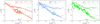 |
Fig. 2 Kinetic energy dependence of the HC3N, HC5N, and HC7N cross-sections induced by collisions with He. Each panel shows the 1 → 0 (solid line) and the 3 → 1 (dashed line) transitions. |
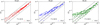 |
Fig. 3 Systematic comparison between the CS and CC rate coefficients (in units of cm3 s−1) induced by collisions with He for a kinetic temperature of 10 K, considering HC3N, HC5N, and HC7N. |
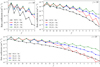 |
Fig. 4 Comparison of the HCN, HC3N, HC5N, and HC7N rate coefficients induced by collisions with He for a kinetic temperature of 10 K. Each panel shows downward transitions out of the indicated rotational level. The data for HCN were computed by Dumouchel et al. (2010). All data shown in this plot were calculated using the close-coupling quantum mechanical approach. |
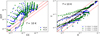 |
Fig. 5 Assessment of the deviation of the collisional rate coefficients (in units of cm3 s−1). The left-hand panel shows the discrepancies generated by the extrapolation method relative to the close-coupling scattering data computed in this work. The right-hand panel compares the HC3N and HC5N, HC3N, and HC7N, and HC5N and HC7N CC rate coefficients. The solid line represents a 1:1 ratio, while the dashed lines delimit a region where the agreement is within a factor of two. |
3 Sensitivity of line intensities to non-LTE effects
The goal of this section is to estimate the impact of the new rate coefficients on the astronomical modelling and to clarify the impact of using extrapolated scattering data and the LTE approximation in investigating the excitation of cyanopolyynes in cold molecular clouds. We performed non-LTE radiative transfer calculations using the escape probability formalism (Goldreich & Kwan 1974), as implemented in the RADEX code (Van der Tak et al. 2007). The molecular data input file is organized into three sections that comprise the rotational energy levels, the Einstein coefficients, and the collisional rate coefficients. For each cyanopolyyne, we obtained the energy levels and Einstein coefficients from the Cologne Database for Molecular Spectroscopy (CDMS) portal (Endres et al. 2016). Regarding collisional rate coefficients, we used various datasets to assess the sensitivity of astronomical lines to the precision of scattering data. Specifically, we employed the CC method and the extrapolated rate coefficients for HC5N and HC7N. Additionally, we used (i) the CC rate coefficients of HC3N as a template for HC5N, (ii) those of HC5N as a proxy for HC7N, and (iii) the scattering data of HC3N to infer those of HC7N. Substituting collisional rate coefficients of cyanopolyynes allows us to predict the effects of using HC7N scattering data to infer those of HC9N and HC11N. Thus, our analysis is based on three non-LTE models4, using the CC-based collisional rate coefficients as a reference. We note that, for HC5N and HC7N, it is possible to use a set of rate coefficients that combine CC data for low energy levels and low temperature, and CS data for high energy levels and high temperature. However, we investigate later the impact of the CS data compared to the CC data. The collisional rate coefficients for HC3N-He, HC5N-He, and HC7N-He were corrected using mass scaling factors of 1.388, 1.396, and 1.400, respectively (Green 1986), to estimate the rate coefficients for HC3N-H2, HC5N-H2, and HC7N-H2. This approximation was suggested as reasonable for HC3N by Wernli et al. (2007), who investigated both He- and H2-induced rate coefficients.
We performed radiative transfer calculations to determine integrated line intensities, hereafter denoted as line intensities, which represent the most practical physical quantities measurable by radio telescopes in molecular observations. The gas kinetic temperature and the molecular hydrogen density were set to T = [5–15] K and n(H2) = [103–105] cm−3, respectively. These temperature and density ranges are broad enough to encompass the physical conditions of the cold media where cyanopolyynes have been detected. For HC7 N, it is worth noting that only the CC set of collisional rate coefficients includes enough energy levels to converge radiative transfer calculations at these temperatures. However, we believe that the limited number of energy levels considered in the approximated collisional datasets is unlikely to alter our analysis. Additionally, we used a column density (N) of 1013cm−2, which is an approximate average N-value for cyanopolyynes reported in the literature. Moreover, our analysis remains unbiased, since we focused on line intensities that are proportional to the column density in the optically thin regime (e.g. Appendix A shows that all the lines are optically thin). For the line width, we applied a value of Δv = 1.0 km s−1, which is unlikely to bias our analysis since the only variable in this study is the set of collisional rate coefficients.
Considering that observational spectra of HC5N and HC7N have often been analysed using either the LTE approximation or a non-LTE approach based on extrapolated rate coefficients, we evaluate the impact of these approximate methods on line intensities of cyanopolyynes. Figure 6 shows the dependence of HC5N and HC7N line intensities on frequency, calculated using different models. For HC5N, the upper panel demonstrates that the LTE approximation slightly underestimates line intensities for transitions below 25 GHz (i.e. j = 0–10) and overestimates those at higher frequencies (v > 35 GHz or j > 13). In the case of HC7N, the pattern is similar. The absence of high-frequency lines results from the use of the CC rate coefficients of HC3N (in the extrapolation), which are limited to transitions between the 26 low-lying rotational levels. A comparison of the left- and right-hand panels reveals that non-LTE effects are less pronounced for HC7N due to its smaller Einstein coefficients.
In the middle panel, where extrapolated rate coefficients are used, the line intensities deviate from the CC-based non-LTE intensities in a similar way to the LTE predictions. For both molecules, the overestimation in line intensity that arises from the LTE approximation (or extrapolated rate coefficients) grows more significantly as the frequency increases, reaching deviations larger than a factor of five (see Appendices B and C that show the same plots for densities of 104 cm−3 and 105 cm−3). It is essential to note that while high-frequency line intensities are typically lower than the dominant ones, their contribution remains crucial for accurate astronomical line modelling. Indeed, when modelling observational spectra, all astronomical line intensities should be accurately reproduced by the non-LTE radiative transfer calculations using the same physical quantities.
Given the reasonable agreement between the high-magnitude collisional rate coefficients of HC3N, HC5N, and HC7N (see Fig. 5), we examine the impact of substituting scattering data on line intensities in the lower panels of Fig. 6. Again, the absence of high-frequency lines in the HC7N case results from using the CC rate coefficients of HC5N, which are limited to transitions between the 26 low-lying rotational levels. Nevertheless, for both molecules, the comparison reveals a strong agreement despite the use of collisional rate coefficients from a different cyanopolyyne in the radiative transfer calculations. We refer the readers to Appendix D, which highlights the consistency of this agreement despite changes in the density and the temperature. This result remains unchanged even when using the collisional rate coefficients of HC3N to infer those of HC7N. This comparison is not shown here, as we obtained the same plot as the one on the right-hand side of the bottom panel of Fig. 6. Therefore, the line intensities of cyanopolyynes exhibit minimal sensitivity to the substitution of collisional rate coefficients between two family members. This can be explained by referring back to Fig. 5, where the high-magnitude rate coefficients – which likely compete with radiative transitions for depopulating molecular energy levels – show good agreement for HC3N, HC5N, and HC7N. Consequently, we anticipate that using the HC7N collisional rate coefficients reported in this work to analyse observational spectra of HC9N and HC11N would yield accuracy within a 10% error margin.
Given the large rotational basis required to converge cross-sections that involves high-lying energy levels (see Table 2), using CC calculations turns out to be highly demanding in terms of CPU time and memory allocation. Therefore, we tested whether CS can be used instead of CC for the high energy levels. The comparison in Fig. 7 shows that the line intensities calculated using the CS rate coefficients align closely with the CC reference calculations. For all three cyanopolyynes, the CC- and CS-based line intensities agree within an error margin of less than 10%. Given the discrepancies between the CC and CS collisional rate coefficients – up to a factor of four for low-magnitude rate coefficients – it appears that the influence of less dominant transitions is minor in the radiative transfer calculations, even for emission lines from high energy levels.
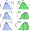 |
Fig. 6 Sensitivity of the HC5N and HC7N line intensities to the accuracy of collisional rate coefficients. Each panel shows the line intensities (∫ TRdυ) and excitation temperatures (Tex) of emission lines as a function of frequency. The physical conditions employed in the calculations are n(H2) = 104 cm−3 and T = 10 K. The superscripts ‘CC’ refers to the close-coupling method used in the calculation of the collisional rate coefficients, whereas ‘R3’ and ‘R5’ denote when we employed the HC3N rate coefficients as template for those of HC5N and the scattering data for HC5N as a proxy for HC7N, respectively. The superscript ‘LTE’ means that the line intensities were derived considering LTE conditions. The shaded region stands for an agreement of 10% with the intensities calculated using CC reference data. |
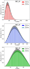 |
Fig. 7 Same as Fig. 6 but including line intensities of HC3N. The superscript ‘CS’ refers to the coupled-states method. |
4 Discussion and conclusions
We calculated the first excitation rate coefficients for HC5N and HC7N induced by collisions with He using quantum mechanical methods. For HC3N, we revisited He-induced scattering, and extended the dataset to include the 26 lowest rotational energy levels.
A comparative analysis of the collisional rate coefficients for HCN (Dumouchel et al. 2010) and the three cyanopolyynes reveals a similar propensity rule for high-magnitude rate coefficients, namely a propensity rule in favour of even Δj transitions. Regarding cyanopolyynes, the high-magnitude collisional rate coefficients – for example, between HC3N and HC5N, HC5N and HC7N, as well as HC3N and HC7N – agree within a factor of two.
We tested the sensitivity of spectral line intensities to non-LTE effects. Specifically, we applied the LTE approximation alongside four non-LTE radiative transfer models based on CC, and extrapolated rate coefficients. The third model involved the use of the rate coefficients of HC3N as a template for HC5N and HC7N, and also the scattering data of HC5N as a proxy for HC7N. The results, with the CC-based calculations as the reference, show that the LTE approximation and the use of extrapolated collision data in radiative transfer calculations overestimate high-frequency line intensities by up to a factor of five. In contrast, the CS-based model and the substitution of collisional rate coefficients between cyanopolyynes yielded line intensities within 10% of the CC-based results. Therefore, the CS approach is reasonable for providing collisional data for cyanopolyynes. For larger cyanopolyynes, we recommend revisiting their abundance using the new scattering data. The minimal impact on line intensity due to the substitution of scattering data between cyanopolyynes suggests that the new HC7N rate coefficients can be used to approximate those of HC9N and even HC11N in astronomical line modelling, with an estimated accuracy of around 10%.
Acknowledgements
The authors acknowledge the European Research Council (ERC) for funding the COLLEXISM project No. 811363, GENCI for awarding us access to the TGCC/IRENE supercomputer within the A0110413001 project, the Programme National “Physique et Chimie du Milieu Interstellaire” (PCMI) of Centre National de la Recherche Scientifique(CNRS)/Institut National des Sciences de l’Univers (INSU) with Institut de Chimie (INC)/Institut de Physique (INP) co-funded by Commissariat a l’Energie Atomique (CEA) and Centre National d’Etudes Spatiales (CNES). F.L. acknowledges the Institut Universitaire de France.
Appendix A Line opacity
Line opacity for the three cyanopolyynes calculated using a gas density of 104 cm−3, a kinetic temperature of 10 K and a column density of 1013 cm−2
Appendix B Line intensity dependence on the LTE approximation: The case of HC5N and HC7N
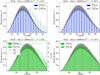 |
Fig. B.1 Same as Fig. 6 but only for the LTE approximation. The physical conditions are shown on top of the panels. |
Appendix C Line intensity dependence on the extrapolated rate coefficients: The case of HC5N and HC7N
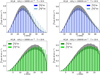 |
Fig. C.1 Same as Fig. 6 but only for the extrapolated rate coefficients. The physical conditions are shown on top of the panels. |
Appendix D Line intensity dependence on the substitution of rate coefficients of different cyanopolyynes: The case of HC5N and HC7N
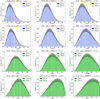 |
Fig. D.1 Same as Fig. 6 but only for the model that uses the rate coefficients of HC3N and HC5N as template for HC5N and HC7N, respectively. The physical conditions are shown on top of the panels. |
Appendix E Line intensity dependence on the CS approximation: The case of HC3N
Appendix F Line intensity dependence on the CS approximation: The case of HC5N
Appendix G Line intensity dependence on the CS approximation: The case of HC7N
References
- Al-Edhari, A. J., Ceccarelli, C., Kahane, C., et al. 2017, A&A, 597, A40 [NASA ADS] [CrossRef] [EDP Sciences] [Google Scholar]
- Alexander, M. H. 1977, J. Chem. Phys., 67, 2703 [NASA ADS] [CrossRef] [Google Scholar]
- Alexander, M. H., & Manolopoulos, D. E. 1987, J. Chem. Phys., 86, 2044 [Google Scholar]
- Alexander, A., Kroto, H., & Walton, D. 1976, J. Mol. Spectrosc., 62, 175 [NASA ADS] [CrossRef] [Google Scholar]
- Bell, M., Feldman, P., Travers, M., et al. 1997, ApJ, 483, L61 [NASA ADS] [CrossRef] [Google Scholar]
- Bell, M., Watson, J., Feldman, P., & Travers, M. 1998, ApJ, 508, 286 [NASA ADS] [CrossRef] [Google Scholar]
- Ben Abdallah, D., Najar, F., Jaidane, N., Dumouchel, F., & Lique, F. 2012, MNRAS, 419, 2441 [NASA ADS] [CrossRef] [Google Scholar]
- Bianchi, E., Remijan, A., Codella, C., et al. 2023, ApJ, 944, 208 [NASA ADS] [CrossRef] [Google Scholar]
- Bop, C. T., & Lique, F. 2024, J. Chem. Phys., 161, 124113 [NASA ADS] [CrossRef] [Google Scholar]
- Chapillon, E., Dutrey, A., Guilloteau, S., et al. 2012, ApJ, 756, 58 [NASA ADS] [CrossRef] [Google Scholar]
- Dumouchel, F., Faure, A., & Lique, F. 2010, MNRAS, 406, 2488 [NASA ADS] [CrossRef] [Google Scholar]
- Dunning Jr, T. H. 1989, J. Chem. Phys., 90, 1007 [NASA ADS] [CrossRef] [Google Scholar]
- Endres, C. P., Schlemmer, S., Schilke, P., Stutzki, J., & Müller, H. S. 2016, J. Mol. Spectrosc., 327, 95 [NASA ADS] [CrossRef] [Google Scholar]
- Fukuzawa, K., Osamura, Y., & Schaefer, H. F. III 1998, ApJ, 505, 278 [NASA ADS] [CrossRef] [Google Scholar]
- Goldreich, P., & Kwan, J. 1974, ApJ, 189, 441 [CrossRef] [Google Scholar]
- Green, S. 1986, ApJ, 309, 331 [NASA ADS] [CrossRef] [Google Scholar]
- Green, S., & Chapman, S. 1978, ApJS, 37, 169 [Google Scholar]
- Hutson, J., & Green, S. 1994, Collaborative computational project [Google Scholar]
- Knizia, G., Adler, T. B., & Werner, H.-J. 2009, J. Chem. Phys., 130, 054104 [Google Scholar]
- Loomis, R. A., Shingledecker, C. N., Langston, G., et al. 2016, MNRAS, 463, 4175 [NASA ADS] [CrossRef] [Google Scholar]
- Loomis, R. A., Burkhardt, A. M., Shingledecker, C. N., et al. 2021, Nat. Astron., 5, 188 [NASA ADS] [CrossRef] [Google Scholar]
- McCarthy, M., Levine, E., Apponi, A., & Thaddeus, P. 2000, J. Mol. Spectrosc., 203, 75 [NASA ADS] [CrossRef] [Google Scholar]
- McGuire, P., & Kouri, D. J. 1974, J. Chem. Phys., 60, 2488 [CrossRef] [Google Scholar]
- Pardo, J., Bermúdez, C., Cabezas, C., et al. 2020, A&A, 640, L13 [NASA ADS] [CrossRef] [EDP Sciences] [Google Scholar]
- Snell, R. L., Schloerb, F. P., Young, J. S., Hjalmarson, A., & Friberg, P. 1981, ApJ, 244, 45 [NASA ADS] [CrossRef] [Google Scholar]
- Thorwirth, S., Müller, H., & Winnewisser, G. 2000, J. Mol. Spectrosc., 204, 133 [NASA ADS] [CrossRef] [Google Scholar]
- Truong, B., Graham, D., Nguyen, Q.-R., et al. 1993, A&A, 277, 133 [NASA ADS] [Google Scholar]
- Van der Tak, F., Black, J. H., Schöier, F., Jansen, D., & van Dishoeck, E. F. 2007, A&A, 468, 627 [NASA ADS] [CrossRef] [EDP Sciences] [Google Scholar]
- Walmsley, C. M., Winnewisser, G., & Toelle, F. 1980, A&A, 81, 245 [NASA ADS] [Google Scholar]
- Werner, H., Knowles, P., Knizia, G., et al. 2015, Version 2015.1, a package of ab initio programs, http://www.molpro.net [Google Scholar]
- Wernli, M., Wiesenfeld, L., Faure, A., & Valiron, P. 2007, A&A, 464, 1147 [NASA ADS] [CrossRef] [EDP Sciences] [Google Scholar]
Explicitly correlated coupled cluster with single, double, and non-iterative triple excitations.
Augmented correlation-consistent polarized valence triple zeta Gaussian basis set.
A channel refers to a specific quantum mechanical state of the system defined by the configuration of the interacting monomers.
Here, a model refers to LTE and non-LTE radiative transfer calculations. In the case of non-LTE calculations, the difference lies in the collisional rate coefficients.
All Tables
Line opacity for the three cyanopolyynes calculated using a gas density of 104 cm−3, a kinetic temperature of 10 K and a column density of 1013 cm−2
All Figures
|
Fig. 1 Low-lying rotational energy levels of HC2n+ıN (n = 1, 2, 3) considered in this work. |
| In the text | |
|
Fig. 2 Kinetic energy dependence of the HC3N, HC5N, and HC7N cross-sections induced by collisions with He. Each panel shows the 1 → 0 (solid line) and the 3 → 1 (dashed line) transitions. |
| In the text | |
|
Fig. 3 Systematic comparison between the CS and CC rate coefficients (in units of cm3 s−1) induced by collisions with He for a kinetic temperature of 10 K, considering HC3N, HC5N, and HC7N. |
| In the text | |
|
Fig. 4 Comparison of the HCN, HC3N, HC5N, and HC7N rate coefficients induced by collisions with He for a kinetic temperature of 10 K. Each panel shows downward transitions out of the indicated rotational level. The data for HCN were computed by Dumouchel et al. (2010). All data shown in this plot were calculated using the close-coupling quantum mechanical approach. |
| In the text | |
|
Fig. 5 Assessment of the deviation of the collisional rate coefficients (in units of cm3 s−1). The left-hand panel shows the discrepancies generated by the extrapolation method relative to the close-coupling scattering data computed in this work. The right-hand panel compares the HC3N and HC5N, HC3N, and HC7N, and HC5N and HC7N CC rate coefficients. The solid line represents a 1:1 ratio, while the dashed lines delimit a region where the agreement is within a factor of two. |
| In the text | |
|
Fig. 6 Sensitivity of the HC5N and HC7N line intensities to the accuracy of collisional rate coefficients. Each panel shows the line intensities (∫ TRdυ) and excitation temperatures (Tex) of emission lines as a function of frequency. The physical conditions employed in the calculations are n(H2) = 104 cm−3 and T = 10 K. The superscripts ‘CC’ refers to the close-coupling method used in the calculation of the collisional rate coefficients, whereas ‘R3’ and ‘R5’ denote when we employed the HC3N rate coefficients as template for those of HC5N and the scattering data for HC5N as a proxy for HC7N, respectively. The superscript ‘LTE’ means that the line intensities were derived considering LTE conditions. The shaded region stands for an agreement of 10% with the intensities calculated using CC reference data. |
| In the text | |
|
Fig. 7 Same as Fig. 6 but including line intensities of HC3N. The superscript ‘CS’ refers to the coupled-states method. |
| In the text | |
|
Fig. B.1 Same as Fig. 6 but only for the LTE approximation. The physical conditions are shown on top of the panels. |
| In the text | |
|
Fig. C.1 Same as Fig. 6 but only for the extrapolated rate coefficients. The physical conditions are shown on top of the panels. |
| In the text | |
|
Fig. D.1 Same as Fig. 6 but only for the model that uses the rate coefficients of HC3N and HC5N as template for HC5N and HC7N, respectively. The physical conditions are shown on top of the panels. |
| In the text | |
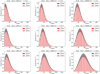 |
Fig. E.1 Same as Fig. 7 but only for HC3N. The physical conditions are shown on top of the panels. |
| In the text | |
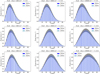 |
Fig. F.1 Same as Fig. 7 but only for HC5N. The physical conditions are shown on top of the panels. |
| In the text | |
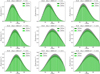 |
Fig. G.1 Same as Fig. 7 but only for HC7N. The physical conditions are shown on top of the panels. |
| In the text | |
Current usage metrics show cumulative count of Article Views (full-text article views including HTML views, PDF and ePub downloads, according to the available data) and Abstracts Views on Vision4Press platform.
Data correspond to usage on the plateform after 2015. The current usage metrics is available 48-96 hours after online publication and is updated daily on week days.
Initial download of the metrics may take a while.