| Issue |
A&A
Volume 698, May 2025
|
|
|---|---|---|
| Article Number | A118 | |
| Number of page(s) | 16 | |
| Section | Galactic structure, stellar clusters and populations | |
| DOI | https://doi.org/10.1051/0004-6361/202453603 | |
| Published online | 06 June 2025 | |
Explaining the 12C/13C ratio in the Galactic halo: The contribution from shell mergers in primordial massive stars
1
Dipartimento di Fisica, Università degli Studi di Trieste,
via Tiepolo 11,
34143
Trieste,
Italy
2
INAF, Osservatorio Astronomico di Trieste,
via Tiepolo 11,
34143
Trieste,
Italy
3
INFN, Sezione di Trieste,
via Valerio 2,
34134
Trieste,
Italy
4
Institute for Fundamental Physics of the Universe,
via Beirut, 2,
34151
Trieste,
Italy
5
Konkoly Observatory, Research Centre for Astronomy and Earth Sciences, HUN-REN,
Konkoly Thege Miklós út 15–17,
1121
Budapest,
Hungary
6
CSFK, MTA Centre of Excellence,
Konkoly Thege Miklós út 15–17,
1121
Budapest,
Hungary
7
INAF, Osservatorio Astronomico di Roma,
Via Frascati 33,
00040
Monteporzio Catone,
Italy
8
INAF/IAPS,
Via Fosso del Cavaliere 100,
00133
Roma,
Italy
9
INFN, Sezione di Perugia, via A. Pascoli s/n,
06125
Perugia,
Italy
10
Monash Centre for Astrophysics (MoCA), School of Mathematical Sciences, Monash University,
Victoria
3800,
Australia
11
Kavli IPMU (WPI), The University of Tokyo, Kashiwa,
277-8583
Chiba,
Japan
12
INAF, Osservatorio Astrofisico di Arcetri,
Largo E. Fermi 5,
50125
Firenze,
Italy
★ Corresponding author: federico.rizzuti@inaf.it
Received:
24
December
2024
Accepted:
25
March
2025
Context. Recent campaigns of observations have provided new measurements of the carbon isotopes in the most metal-poor stars of the Galaxy. These stars are so metal-poor that they could only have been enriched by one or few generations of massive progenitors. However, explaining the primary production of 13C and the low 12C/13C ratio measured in these stars is challenging.
Aims. Making use of the most up-to-date models for zero-metal and low-metallicity stars, we investigate possible sources of 13C at low metallicity and verify whether massive stars could be solely responsible for the 12C/13C ratio observed in halo stars.
Methods. We employed the stochastic model for Galactic chemical evolution GEMS to reproduce the evolution of CNO elements and 12C/13C ratio, including the enrichment from rotating massive stars, some of which show the occurrence of H-He shell mergers.
Results. We find that stars without H-He shell mergers do not produce enough 13C to be compatible with the observations. Instead, primary production via shell mergers and subsequent ejection during the supernova explosion can explain a ratio of 30 <12C/13C < 100. The observations are best reproduced assuming a large frequency of shell mergers. A ratio of 12C/13C < 30 can only be reproduced by assuming an outer layer ejection and no explosion, but requiring a higher level of production of 12C and 13C.
Conclusions. Zero-metal and low-metallicity spinstars with H-He shell mergers appear as the most plausible scenario to explain the low 12C/13C ratio in carbon-enhanced metal-poor (CEMP) stars. The entire range of 12C/13C values can be explained by assuming that some stars fully explode, while others only eject their outer layers. Shell mergers are also expected to be more frequent and productive, which is allowed by the current uncertainties related to the treatment of convection in stellar modelling.
Key words: nuclear reactions, nucleosynthesis, abundances / stars: massive / stars: Population III / stars: rotation / Galaxy: abundances / Galaxy: evolution
© The Authors 2025
 Open Access article, published by EDP Sciences, under the terms of the Creative Commons Attribution License (https://creativecommons.org/licenses/by/4.0), which permits unrestricted use, distribution, and reproduction in any medium, provided the original work is properly cited.
This article is published in open access under the Subscribe to Open model. Subscribe to A&A to support open access publication.
1 Introduction
The old and metal poor stars that compose the Galactic halo possess critical information about the initial phases of galaxy evolution (Chamberlain & Aller 1951; Bessell & Norris 1984; Beers et al. 1985). Indeed, while zero-metal stars (also known as Population III or Pop III stars) have never been directly observed (presumably because stellar formation is biased towards short-lived massive stars at lower metallicity), many of the oldest stars in the Galactic halo have such low levels of metal content that they are believed to have formed from the explosion of Pop III stars as type-II supernovae (SNe II). As a result, this process could have locked in the new stellar atmosphere the chemical composition processed by only one generation of primordial stars. These second-generation stars with subsolar masses survived until today, representing some of the oldest and most metal-poor stars that can be observed in the Milky Way (see Aguado et al. 2023).
Recent spectroscopic surveys continue to provide thousands of high-resolution spectra for metal-poor halo stars (York et al. 2000; Keller et al. 2007; Yanny et al. 2009; Deng et al. 2012; Caffau et al. 2013; Starkenburg et al. 2017; Rockosi et al. 2022). Considering that direct detection of Pop III stars from primordial galaxies at high redshift is still unviable, the abundance measurements of metal-poor halo stars represent the only way of constraining the properties and nucleosynthesis of the first generation of stars.
Ever since the first surveys of metal-poor halo stars (Beers et al. 1985) and the first spectroscopic follow-ups (Molaro & Castelli 1990; Molaro & Bonifacio 1990), a large fraction of stars was found to be highly enriched in carbon (Beers et al. 1992), compared to the solar value ([C/Fe] > 0.7). These carbonenhanced metal-poor (CEMP) stars represent the totality of stars at metallicity [Fe/H] < −5, and only two stars out of 14 known at [Fe/H] < −4.5 have normal solar abundance. Some CEMP stars also show the presence of neutron-capture elements in their atmospheres, while others do not: when [Ba/Fe] > 1, these are called CEMP-s stars; whereas if [Ba/Fe] < 0, they are considered CEMP-no stars. CEMP-no stars outnumber CEMP-s below [Fe/H] < −2.3 (Yoon et al. 2018). For CEMP-no stars, it is believed that the large carbon abundance comes from the gas in which the star formed that had previously been enriched by Pop III stars; however, to explain CEMP-s stars, the presence of an asymptotic giant branch (AGB) companion is typically invoked, which accretes both carbon and s-process elements onto the CEMP star. The two classes also exhibit different levels of carbon (Spite et al. 2013; Bonifacio et al. 2015) and almost all CEMP-s stars are found in binary systems (Lucatello et al. 2005; Starkenburg et al. 2014).
Explaining the chemical composition and large carbon enrichment of CEMP-no stars has always been challenging. Carbon is a primary element that is produced in both massive and low-intermediate mass stars (LIMS). Considering that CEMP-no stars are the result of a few or even just one progenitor, their composition must be explained either by a single source abundant in carbon, but scarce in iron (Umeda & Nomoto 2003), or multiple sources whose ejecta are enriched in light elements and that pollute a small region (Bonifacio et al. 2003; Chieffi & Limongi 2003). Overall, the mechanisms that determine the explosion of massive stars as type-II supernovae are still not completely understood, given the interplay of several complex phenomena (Müller & Janka 2015; Perego et al. 2015; Curtis et al. 2019; Burrows & Vartanyan 2021; Boccioli & Roberti 2024). It has been constrained from observations (since Sollerman et al. 1998; Turatto et al. 1998) that SNe II must possess a distribution of explosion energies, in some cases ejecting very low masses of iron. These so-called ‘faint SNe’ represent an excellent candidate for explaining the nature of CEMP-no stars, since they eject a small amount of Fe but large amounts of CNO elements (Bonifacio et al. 2003; Chieffi & Limongi 2003; Umeda & Nomoto 2003, 2005).
CEMP-no stars are also interesting sites for exploring the behaviour of the isotopic ratio 12C/13C. Normally, 13C is produced in H-burning regions by the CNO cycle, but it is later destroyed during the evolution of the star. A possible way of producing and preserving superficial 13C is in AGB stars due to hot bottom burning or hot-third dredge up that leads to H-burning at the bottom of the convective envelope (Renzini & Voli 1981; Busso et al. 1999; Cristallo et al. 2009, 2011; Karakas 2010). However, a low 12C/13C ratio, therefore large amounts of 13C, has been often observed in CEMP-no stars (Spite et al. 2006, 2021), which are so metal-poor that only massive stars could have contributed to their enrichment. This requires 13C to be produced as a primary element at low metallicity, as is the case for 14N. In fact, Matteucci (1986) first showed that nitrogen requires a primary production by massive stars, so the same is expected to be valid for 13C (see also Romano & Matteucci 2003).
A possible path for 13C production is when H- and He-burning regions get in contact at late times in the stellar evolution. Mixing episodes between H- and He-burning regions have been reported in stellar modelling for a long time, especially for massive zero-metal stars (Woosley & Weaver 1982; Heger & Woosley 2010; Limongi & Chieffi 2012). The subsequent introduction of rotation in stellar modelling (Meynet & Maeder 2002; Ekström et al. 2008) has even enhanced these effects, due to the rotation-induced mixing. Motivated by observations of low 12C/13C in unmixed stars (Spite et al. 2006), Hirschi (2007) has shown that a low 12C/13C ratio can be obtained in massive fast rotators (vini = 600–800 km s−1) down to Z = 10−8. This is possible thanks to the rotational mixing that transports carbon from the He-burning core up to the tail of the H-burning shell, thereby producing primary 13C and 14N. This has been confirmed and further explored by Choplin et al. (2017). A similar production of 13C also in absence of rotation has been shown to be possible in massive zero-metal stars (Limongi & Chieffi 2012; Clarkson & Herwig 2021), due to convection-induced mixing and proton ingestion into He-burning regions (see also Herwig et al. 2011). The two mechanisms of rotation- and convection-induced mixing can also co-exist (Roberti et al. 2024).
These occurrences are sometimes called ‘shell mergers’ in cases when the H- and He-burning shells are sufficiently close to each other that convection overcomes the inter-shell barrier and material can mix between the two shells, sometimes merging into a new single convective region. The H-rich material is entrained and burns with the C of the He-burning shell, producing 13C and 14N, and then it is transported close to the surface by the strong convection of the shell merger, later enriching the ISM. The occurrence of shell mergers in massive stars and their frequency are still largely debated, but recent indications from both 1D and multi-D stellar models show that they may occur quite often (Sukhbold & Woosley 2014; Collins et al. 2018; Roberti et al. 2024; Rizzuti et al. 2024). H-He shell mergers are more common at low metallicity due to the smaller entropy jump between the shells and partial activation of the 3α process, making the shells closer both in mass and in radius (see e.g. Roberti et al. 2024).
Overall, rotation is believed to play a key role in Pop III stars. Stellar modelling has been showing (Meynet & Maeder 2002; Hirschi 2007; Frischknecht et al. 2016; Limongi & Chieffi 2018) that massive stars at low metallicity are expected to have higher rotation velocity, due to their lower opacity, larger compactness, and lower mass loss. Fast metal-poor rotators have been used in studies of Galactic archaeology to explain both light and heavy element production at low metallicity (since Chiappini et al. 2006, 2008; Cescutti & Chiappini 2010; Cescutti et al. 2013), thanks to the rotation-induced mixing that affects the core size and transports the products closer to the surface. These same mechanisms may also have a key role for explaining the carbon enhancement of CEMP-no stars.
Indeed, Galactic archaeology represents a precious method to validate stellar modelling results, by relating the yields from stellar models to the actual observations. Chiappini et al. (2008) were first to show that using the yields of Hirschi (2007), a very low 12C/13C ~ 30 can be reached at low metallicity thanks to fast rotators employed in a chemical evolution model. More recently, Romano et al. (2017, 2019) and Prantzos et al. (2018) confirmed and further investigated these results, employing more recent grids of rotating massive stars (see also Romano 2022). The recent measurements of 12C/13C in increasingly lower metallicity stars (Aguado et al. 2022; Molaro et al. 2023) further motivate the research of their production sites.
In this paper, we present the results from a stochastic chemical evolution model of the Galactic halo, including the nucleosynthesis from zero-metal and metal-poor stars, to explain the production of CNO elements and the 12C/13C ratio recently measured in halo stars.
The paper is organised as follows. In Section 2, we list the adopted observations. In Section 3, we present the chemical evolution model. In Section 4, the nucleosynthesis prescriptions are discussed. In Section 5, the results are presented. In Section 6, our conclusions are drawn.
Observational data used for this work: source, number of giants (defined as log g < 3.2), number of dwarfs (log g ≥ 3.2), method of analysis, spectral resolution, and abundances used.
2 Observations
In this paper, we reproduce the chemical evolution of the isotopes of carbon and the elements nitrogen, oxygen, barium, and strontium for stars in the Galactic halo. Given that these abundances are measured in stellar atmospheres with different methods, here we rely on multiple works that include measurements of the most metal-poor stars in the literature.
We present in Table 1 the observations we employ in this work, listing the number of giants and dwarfs, with details of their analysis. We are aware that the original surface abundances of a star can be modified at the end of its lifetime, due to internal mixing processes during the red giant phase, such as first dredge-up and thermohaline mixing (Marini et al. 2023; Mohorian et al. 2024; Nguyen et al. 2025). This mainly affects the light elements, while the heavy elements are mostly left untouched. In order to avoid this source of uncertainty, we only include dwarf stars in our CNO observation sample, selected on the basis of their having log g ≥ 3.2. Some exceptions include studies that provide evolutionary corrections for C in giants (Placco et al. 2014) or that use Li to detect unmixed giants (Spite et al. 2005). For Sr and Ba, we included giants instead. We also present in the appendix the Kiel diagram of the observations (Fig. A.1). In particular, Placco et al. (2014) provided a compilation of observations for C, N, Sr, and Ba (see references within), including an evolutionary correction for C to recover its original surface abundance in red giant branch (RGB) stars.
Oxygen is particularly challenging to measure in stars with low metallicity. We include measurements for C, N, and O from the works of Israelian et al. (2004); Spite et al. (2005); Lai et al. (2008); Fabbian et al. (2009); Norris et al. (2013); Zhao et al. (2016). The observations of Fabbian et al. (2009) and Zhao et al. (2016) have been obtained with non-LTE analysis. Spite et al. (2005) have corrected their observations for 3D effects by −0.40 for nitrogen (NH band) and by −0.23 for oxygen ([O I] line). Then, Sr and Ba at intermediate metallicity come from the MINCE project by Cescutti et al. (2022); François et al. (2024).
For 12C and 13C, we employed the compilation of stars presented in the recent work of Molaro et al. (2023), which also includes new measurements for six stars among the most metal-poor known in the halo, in addition to a list of measurements from previous works1. We also include the dwarf stars HD 140283 from Spite et al. (2006, 2021) and HE 0007-1832 from Cohen et al. (2004). It is important to highlight that six stars in our sample with 12C/13C < 30 are dwarfs; therefore, their low 12C/13C is not an effect of internal mixing: CS 22887-048, CS 22945-017, CS 22956-028, CS 22958-042, G77-61, and HE 0007-1832.
We adopted in our models the solar abundances of Asplund et al. (2009). This is not always the case for the observations listed above, especially works published before 2009 based on a range of prescriptions (see each work). Overall, these very small differences do not invalidate the comparison of the models to the observations.
3 Chemical evolution model
For this work, we have developed a new version of the stochastic model first presented in Cescutti & Chiappini (2010), which was based on the inhomogeneous model of Cescutti (2008) and on the homogeneous model of Chiappini et al. (2008). The stochastic model has been introduced to reproduce the scatter visible in the observations of neutron-capture elements at low metallicity, which can be explained by the randomly distributed physical properties of the stars (Cescutti et al. 2013; Cescutti & Chiappini 2014; Cescutti et al. 2016; Rizzuti et al. 2021). In this sense, chemical evolution models that take this dispersion into account have additional degrees of freedom that can be used to further constrain the stellar properties (see also Tsujimoto et al. 1999; Ishimaru & Wanajo 1999; Travaglio et al. 2001; Argast et al. 2002, 2004; Karlsson & Gustafsson 2005; Wehmeyer et al. 2015).
We have further developed the stochastic model by adapting the code to parallel computing, using domain decomposition through the message-passing-interface (MPI) library for inter-process communication. This allowed us to dramatically increase the number of volumes used to simulate the Galactic halo. We also expanded the list of isotopes and added to the code new sources of nucleosynthesis for zero-metal and low-metallicity stars (see Section 4). We named this new release of the stochastic model GEMS (Galactic Evolution via Montecarlo Sampling).
We recall here that the model was constructed to reproduce the chemical history of the Galactic halo; therefore, it runs for 1 Gyr after the formation of the Galaxy. To reproduce the inhomogeneities in the chemical composition, the simulation domain was divided into sub-volumes, which are considered to be independent. Each cell was assumed to be a cube of volume 8 × 10⁶ pc3 as in Cescutti et al. (2015) to take into account the distance covered by the ejecta of supernovae (~50 pc, Thornton et al. 1998), so to avoid exchange of material between cells. Taking a volume too large would reduce the stochasticity and produce more homogeneous results. On the other hand, the metallicity that we are trying to reproduce is extremely low; thus, there are very few events that could be behind the enrichment before reaching a higher metallicity. For this reason, we had to drastically increase the number of volumes in the simulation, going from 100 of Cescutti (2008) and 1000 of Cescutti et al. (2016) to 10 000 volumes in this work; this was done thanks to the parallel computing of the GEMS code. Despite the large number of cells, the total volume of our simulations still represents only less than 0.1 per cent of the total volume of the Galactic halo.
The model we employed here has the same specifics described in Rizzuti et al. (2021). In particular, we recall that only one infall episode is assumed for the halo, accreting gas of primordial composition according to a Gaussian distribution (Chiappini et al. 2008):
![$\[\dot{G}(t)_{\mathrm{inf}}=\frac{\Sigma_{\mathrm{h}} ~A}{\tau \sqrt{2 \pi}} \mathrm{e}^{-\left(t-t_0\right)^2 / 2 \tau^2},\]$](/articles/aa/full_html/2025/06/aa53603-24/aa53603-24-eq1.png) (1)
(1)
where t0 is 100 Myr, τ is 50 Myr, and the normalisation is given by Σh = 80 M⊙ pc−2 and A the surface of each cell, so that Σh A = 3.2 × 10⁶ M⊙. The initial mass function (IMF) ϕ(m) adopted here is the one from Scalo (1986). The star formation rate (SFR) in units of M⊙ Gyr−1 is defined as
![$\[\psi(t)=\nu \Sigma_{\mathrm{h}} ~A\left(\frac{G_{\mathrm{gas}}(t)}{\Sigma_{\mathrm{h}} ~A}\right)^k,\]$](/articles/aa/full_html/2025/06/aa53603-24/aa53603-24-eq2.png) (2)
(2)
where ν is 1.4 Gyr−1 k equals 1.5, and Ggas(t) is the amount of gas inside the volume in M⊙.
Finally, we take into account the Galactic wind that takes gas out of each cell, with a rate that is proportional to the star formation rate:
![$\[\dot{G}(t)_{\text {out }}=\omega ~\psi(t),\]$](/articles/aa/full_html/2025/06/aa53603-24/aa53603-24-eq3.png) (3)
(3)
according to a constant ω set equal to 8 for all chemical species (Chiappini et al. 2008).
The evolution proceeds in the following way. In order to ensure stochasticity, in each cell at each time step, a certain mass of gas (according to the SFR) is converted into stars, which are randomly extracted with mass between 0.1 and 100 M⊙. In this way, each cell has the same amount of stars in mass but with a different distribution. After the stars are born, their evolution is followed until they die, assuming the stellar lifetimes of Maeder & Meynet (1989).
4 Nucleosynthesis prescriptions
As we mention in the introduction, to explain the CNO abundances and 12C/13C ratio observed in halo stars, we need to assume specific nucleosynthesis sources. In the GEMS code, the productive sources considered for the chemical enrichment are LIMS and rotating massive stars, with their endpoints being AGB stars, type-Ia SNe, core-collapse SNe, and neutron star Article number, page 4 of 16 mergers. Although all these sources are present in the model, to explain the low-metallicity observations at [Fe/H] < −2, only sources with short time-scales are predominant, in particular, massive stars and their supernova explosions. We list the nucleosynthesis assumptions we included in the model below.
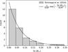 |
Fig. 1 Number distribution of ejected Fe mass from low-metallicity SNe, estimations from Tominaga et al. (2014) (histogram) and exponential fitting (dashed line) used to reproduce faint SNe. |
4.1 Faint supernovae and iron
Over the years, the observations of CEMP stars with very low iron content but high carbon suggested the existence of stars that explode as so-called ‘faint SNe’ (Bonifacio et al. 2003; Chieffi & Limongi 2003; Umeda & Nomoto 2003, 2005; Tominaga et al. 2007, 2014; Nomoto et al. 2013). These events have been introduced to reproduce the abundance patterns and other observational data from peculiar stars and SN remnants (Sollerman et al. 1998; Turatto et al. 1998). It is assumed that a large amount of mixing and fallback in the inner layers prevents the star from ejecting most of its Fe, but still allows it to eject the outer layers rich in CNO elements. Compared to standard core-collapse SN that have an explosion energy of ~1051 erg, 3D SN simulations are also able to reproduce low-luminosity explosions, reaching energies <1050 erg (Stockinger et al. 2020; Kozyreva et al. 2022).
Since we know very little of the physics and distribution of these faint SNe, we formulate here some prescriptions based on observational constraints. Cescutti et al. (2016), when implementing faint SNe in their chemical evolution model, assumed a linear distribution of Fe yields from zero to 0.2 M⊙, therefore with an expected value of 0.1 M⊙. We use here a different approach: Tominaga et al. (2014) constrained the nucleosynthesis of faint SNe by producing SN models that reproduce the abundance patterns of 48 stars with [Fe/H] < −3.5. It can be noticed (see Fig. 1) that the distribution of ejected Fe mass roughly follows an exponential probability distribution:
![$\[f(x ; \beta)= \begin{cases}\frac{1}{\beta} \mathrm{e}^{-x / \beta} & x \geq 0, \\ 0 & x<0,\end{cases}\]$](/articles/aa/full_html/2025/06/aa53603-24/aa53603-24-eq4.png) (4)
(4)
which can be fitted so that the expected value E[X] = β is around 0.07, as expected from core-collapse SN.
In this study, we assume that core-collapse SNe eject an amount of Fe mass following distribution (4), with β the Fe yield given by the stellar evolution model. The yields assumed for Fe come from the same models of massive stars that produce the CNO elements (see next section). We note that with this approach, faint SNe always eject some iron, even if only a few percent of a regular supernova. This means that most of the other elements are also ejected, in particular, the CNO elements produced close to the surface; this is necessary in order to reproduce CEMP-no stars with abundant C and low (but non-zero) Fe. The scenario of a faint supernova is different from the one of a ‘failed’ supernova, where – despite the unsuccessful explosion – it is still possible that only the outer layers are ejected, which are enriched in light elements, but no iron.
4.2 Stellar yields for C, N, O
Carbon, nitrogen, and oxygen can be produced by stars of different masses; therefore, their time-scale of production is dependent on the lifetime and mass of the star. For the metallicity range we are most interested in ([Fe/H] < −2), the main producers are the massive stars (M > 8 M⊙). Non-rotating stellar yields traditionally used in chemical evolution studies (e.g. Woosley & Weaver 1995) have been shown to underestimate the production of both light and heavy elements (e.g. Cescutti et al. 2016; Romano 2022; Rossi et al. 2024). Instead, rotation has been shown to have a critical impact on the stellar nucleosynthesis (Meynet & Maeder 2002; Hirschi 2007), especially at low metallicity, where stars are more compact due to their lower opacity and tend to rotate faster. Additionally, rotating massive stars are the only way to explain the production of primary 13C and 14N observed in low metallicity stars (Chiappini et al. 2006, 2008).
Recently, several works have produced grids of models for rotating massive stars at low metallicity, providing stellar yields to be used for Galactic archaeology (Hirschi 2007; Frischknecht et al. 2012, 2016; Limongi & Chieffi 2018; Roberti et al. 2024). In particular, the stellar models produced with the FRANEC code (Chieffi & Limongi 2013) represent one of the most complete grids of models in the literature. Among their strengths are their treatment of rotation, evolution until the pre-SN stage, and explosive nucleosynthesis. Limongi & Chieffi (2018) provide a grid of nine masses between 13–120 M⊙, four metallicities [Fe/H] = 0, −1, −2, and −3, and three rotations with an initial equatorial velocity of 0 km s−1 (non rotating), 150 km s−1, and 300 km s−1. This grid of models has proved to be extremely interesting for the recent developments in chemical evolution studies (Prantzos et al. 2018, 2023; Romano et al. 2019; Rizzuti et al. 2019; Grisoni et al. 2020; Kobayashi 2022; Molero et al. 2023; Rossi et al. 2024).
The yields of Limongi & Chieffi (2018) have been also implemented in the stochastic model of Rizzuti et al. (2021), which is at the basis of the GEMS code presented here. Although the basic implementation remains the same, there are important differences that it is worth underlining here. Limongi & Chieffi (2018) provide different sets of yields, depending on the physical assumptions. Differently from Rizzuti et al. (2021), we used here their Set R (recommended), calculated using the mixing and fallback technique (Umeda & Nomoto 2003, 2005) assuming that each star ejects 0.07 M⊙ of 56Ni, but stars >25 M⊙ fully collapse to a black hole, therefore enriching the ISM only of wind during their lifetime. This assumption is consistent with observations of red supergiants in the Local Group with masses up to 25 M⊙ (Smartt et al. 2009), and theoretical studies failing to explode stars above 25–30 M⊙ (Sukhbold et al. 2016; Müller et al. 2016; Chieffi & Limongi 2020; Boccioli et al. 2023); however, we recognise that this threshold of explodability is still an open problem and subject to uncertainty. Having only wind contribution from stars >25 M⊙ and not the explosion decreases the enrichment in almost all elements. Considering that fast rotation enhances the nucleosynthesis instead, the net effect is that low-metallicity stars are required to rotate faster to produce the same enrichment. The exact rotation velocity function we assume is described below.
To reproduce the observations below [Fe/H] = −3, which is the lowest metallicity in the Limongi & Chieffi (2018) grid of stellar models, we extended the grid with the recent work of Roberti et al. (2024), who also employed the FRANEC code, providing 15 and 25 M⊙ models at [Fe/H] = −4, −5, and zero metal (Z = 0) for a wide range of rotation velocities. Although partial, this grid proves to be crucial for our investigation. We complement the grid in the following way: stars between 8 and 15 M⊙ have the same nucleosynthesis as 15 M⊙, those between 15 and 25 M⊙ are linearly interpolated, and for those above 25 M⊙, we assume no production, considering that we expect only a wind contribution, which is always several orders of magnitude lower than the explosive one. It should be noticed that most 15 M⊙ models have C-O shell mergers, which affect the abundances in the inner layers (see Roberti et al. 2024).
Finally, the GEMS code includes also the contribution from LIMS, whose impact is visible in the model results only from around [Fe/H] > −2. The yields have been assumed from stellar models obtained from the FRUITY database (Cristallo et al. 2009, 2011, 2015) for non-rotating stars between 1.3–6 M⊙.
4.3 Stellar yields for neutron capture elements
Massive stars are important producers of both light and heavy elements; in particular, they can also produce trans-iron nuclei when rotation is taken into account, thanks to the s-process enabled by rotational mixing between the H-shell and He-core (Frischknecht et al. 2012, 2016; Chieffi & Limongi 2013; Limongi & Chieffi 2018). The present work is not focused on studying the evolution of neutron-capture elements, since this has already been done by Rizzuti et al. (2021) with very similar assumptions. However, in changing the implementation of massive stars to reproduce the CNO elements, we are also changing the production of s-elements, since they come from the same sites. A holistic approach to Galactic archaeology would require the same chemical evolution model to reproduce the evolution of multiple elements under the same assumptions, rather than fine-tuning every time the individual elements. For these reasons, we show in this paper also the predicted evolution of heavy elements strontium and barium, after the model has been fine-tuned to explain the CNO isotopes. In this way, we intend to show that the model does not have to be calibrated again to explain the evolution of different elements, but a convergence of results over the same assumptions is achievable.
A detailed description of the neutron-capture nucleosynthesis and its implementation in the stochastic model has already been presented in Rizzuti et al. (2021). We recall here that the production of heavy elements requires multiple sources, namely rotating massive stars (s-process) and neutron star mergers or magneto-rotationally driven SNe (r-process) at lower metallicity, and AGB stars (s-process) at higher metallicity. The stellar yields we employ come from the same sources described in the previous sections; however, for LIMS the yields from non-rotating models tend to overproduce the neutron capture elements at solar metallicity, while rotating models have too little production instead. Therefore, as already done in Rizzuti et al. (2019, 2021), we divide the non-rotating yields by a factor of 2, so that the abundance of neutron capture elements observed at solar metallicity can be reproduced.
Neutron star mergers are implemented in the GEMS code to reproduce the r-process production of heavy elements. Their implementation is described in Cescutti et al. (2015), in particular, the productive mass range is 9–50 M⊙, the fraction of binary systems is 0.018, and the coalescence time-scale is fixed to 1 Myr, consistently with what found by Matteucci et al. (2014). The assumption of a constant time-delay is simplistic, considering that more complex prescriptions have been developed in the recent years (Simonetti et al. 2019; Molero et al. 2021; Cavallo et al. 2021). However, it can still reproduce the observations, and the question of the productive sites for the r-process is still largely debated today. In particular, our models show that below [Fe/H] < −3 the s-process from massive stars dominates the production of Sr and Ba, while from [Fe/H] > −3 a mixture of s- and r-process is responsible (see also Cescutti & Chiappini 2014).
4.4 Rotation velocity in massive stars
To reproduce neutron-capture elements measured in halo stars, Rizzuti et al. (2021) have calibrated the rotational velocity of low-metallicity massive stars through observations assuming a distribution in rotational velocities. Given that only three rotations are provided in the Limongi & Chieffi (2018) grid, Rizzuti et al. (2021) used interpolation between different velocities. Here, we improve the study by extending the grid of stellar models below [Fe/H] = −3. A new calibration would be required at this point, similar to what was done in Rizzuti et al. (2021), for the new yields and assumptions. However, the stellar grid that we use below [Fe/H] = −3 (i.e. Roberti et al. 2024) is still incomplete in mass. For this reason, we make here the simplest assumptions to avoid additional sources of uncertainty.
We assume the same rotation velocity for stars with the same mass and metallicity so that we do not interpolate between stellar models with different rotations, given the possible non-linearity of stellar physics. Therefore, we give all massive stars the same rotation velocity depending on their metallicity:
![$\[\text { velocity }([\mathrm{Fe} / \mathrm{H}])= \begin{cases}300 \mathrm{~km} \mathrm{~s}^{-1} & {[\mathrm{Fe} / \mathrm{H}] \leq-3}, \\ 150 \mathrm{~km} \mathrm{~s}^{-1} & {[\mathrm{Fe} / \mathrm{H}]>-3}.\end{cases}\]$](/articles/aa/full_html/2025/06/aa53603-24/aa53603-24-eq5.png) (5)
(5)
This distribution is inspired by the assumptions and results of Prantzos et al. (2018) and Rizzuti et al. (2021), but considering a faster rotation to compensate for the enrichment only by winds above 25 M⊙. We are interested here only in metal-poor stars below [Fe/H] < −2, therefore we do not decrease the rotation even further towards solar metallicity, as discussed in Rizzuti et al. (2019).
5 Results
5.1 The 12C/13C ratio in stellar models
As a first step towards explaining the 12C/13C ratio measured in halo stars, we present here a detailed analysis of the stellar yields produced by some of the most recent studies on stellar modelling. The abundances observed in extremely metal-poor halo stars ([Fe/H] ≤ −3) suggest that the gas that formed them had been enriched only by a few generations of progenitors, if not directly from zero-metal stars. This means that the contribution to the chemistry of those stars can only come from massive stars, which are the first to die and enrich the ISM. Therefore, we need to identify the possible stellar models of massive stars that produce the correct amount of 12C and 13C actually observed in metal-poor stars. We remind that all the massive star models we analyse in this work provide explosive yields, assuming that both inner and outer layers of the star are ejected; we treat the case of partial ejection in Section 5.3. All 12C/13C ratios we compute and show in this paper are abundances by number.
Limongi & Chieffi (2018) have developed a set of models with different mass, metallicity, and rotation velocity (see Section 4). We compute and show in Fig. 2 the 12C/13C ratio for all these models, grouped by mass and rotation velocity. In particular, the first row of Fig. 2 shows the masses 13 – 25 M⊙, that in Limongi & Chieffi (2018) contribute via both wind and explosion, while the 30–120 M⊙ stars in the second row only contribute via stellar wind. The observations of halo stars presented in Section 2 all measure a 12C/13C ratio below 100. We can clearly see from Fig. 2 that stellar models between 13–25 M⊙ (first row) all predict a 12C/13C ratio well above 100, due to their very small production of 13C. On the other hand, a few more massive stars that only enrich through the wind (Fig. 2, second row) can reach 12C/13C <100. However, the amount of 13C ejected is very small (<10−3 M⊙ for [Fe/H] = −3), and the birth of stars >25 M⊙ is disfavoured compared to less massive stars, so their enrichment would soon be mixed with 12C-rich material from SN ejecta, and the 12C/13C ratio would greatly increase.
Therefore, the Limongi & Chieffi (2018) stellar models down to [Fe/H] = −3 cannot reproduce the 12C/13C ratio measured from observations, which are mostly below [Fe/H] < −3 and would require extrapolation of the yields at lower metallicity. This implies that a different mechanism of production for 13C is necessary at extremely low metallicity.
As we introduced in Section 4, a new set of FRANEC models has been published by Roberti et al. (2024), exploring 15 and 25 M⊙ stars at metallicity [Fe/H] = −4, −5, and zero metals (Z = 0), for many different rotation velocities. Despite its much smaller mass range, its extremely low metallicity and large rotation range make this grid ideal for investigating the nucleosynthesis of the first stars. Similarly to what we did before, we show in Fig. 3 the 12C/13C ratio as predicted by the models of Roberti et al. (2024), plotted as a function of the stellar initial equatorial velocity. It can be noticed that, despite some exceptions, generally a faster rotation corresponds to lower 12C/13C, therefore a larger production of 13C, up to around 10−3 M⊙. This is due to the ‘entanglement’ effect described in Roberti et al. (2024): the rotation-induced instabilities encourage the exchange of matter between the He-core and the H-shell, resulting in a larger concentration of CNO products in the core and stable intershell, including 13C. Later on, He-core and He-shell burning completely destroy the 13C through (α, n). Indeed, we see from Fig. 3 that most models lie above 12C/13C > 103, indicating that this mechanism does not leave much 13C. However, there are a few models that lie below 12C/13C < 103, with some of them even below 12C/13C < 102. This larger production of 13C is the result of another type of occurrence.
In Roberti et al. (2024), the non-rotating 25 M⊙ models at [Fe/H] = −5, −∞, and the 300 km s−1 rotating one at [Fe/H] = −∞ (the ones with lowest 12C/13C in Fig. 3, right) present a merging of the outer H-burning shell with the He-burning shell immediately below. In particular, once the He-shell penetrates upwards into the H-shell, the rapid engulfment of protons heating at He-burning temperature produces large amounts of 13C and 14N. Part of these products, instead of being immediately burnt, are convectively transported outside the He-burning region to the outer layers of the shell merger, where they can survive. This mechanism explains the large 13C production (up to 10−2 M⊙) and low 12C/13C ratio. These are the yields that we employ in the chemical evolution model in order to explain the observed 12C/13C ratio in halo stars.
To shed more light on the effects of H-He shell mergers on the 13C production, we analyze also the results of Limongi & Chieffi (2012), who presented a set of non-rotating zero-metal models in the range 13–80 M⊙. The aim is to draw a comparison with the grid of models by Roberti et al. (2024), although only for non-rotating massive stars. We show in Fig. 4 the predicted 12C/13C in Limongi & Chieffi (2012) versus Roberti et al. (2024) as a function of the initial stellar mass. Although Roberti et al. (2024) has modelled only two masses, results seem compatible between the two studies. Only stars with mass between 25–35 M⊙ exhibit the H-He shell merger described above, resulting in large production and expulsion of 13C. These results support our choice of including shell merging events in our chemical evolution model.
Finally, to interpret the behaviour of the model above [Fe/H] = −2, we also briefly present the nucleosynthesis sources that contribute at higher metallicity, i.e. LIMS. We plot in Fig. 5 the 12C/13C ratio from the non-rotating 1.3–6 M⊙ stellar models of Cristallo et al. (2009, 2011, 2015) that we use in the GEMS code. We can immediately notice that the ratio spans a wide range across ~20–20 000 at low metallicity, which gradually reduces going towards solar metallicity. Their impact on the chemical evolution is shown in the next sections.
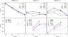 |
Fig. 2 12C/13C ratio in the stellar models of Limongi & Chieffi (2018), for stars that contribute via both wind and explosion (first row) or only wind (second row), for the three initial rotation velocities 0 (left), 150 (centre) and 300 (right) km s−1. Where dots are missing the models do not predict enrichment of 12C or 13C, or both. |
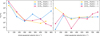 |
Fig. 3 12C/13C ratio in the stellar models of Roberti et al. (2024), for 15 (left) and 25 M⊙ (right) stars, as a function of the star initial equatorial velocity in km s−1. Different colours correspond to different metallicities: [Fe/H] = −4, −5 and −∞ (zero metals). |
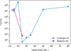 |
Fig. 4 12C/13C ratio in the stellar models of Limongi & Chieffi (2012) compared to Roberti et al. (2024), as a function of the stellar mass, for non-rotating zero-metal stars. |
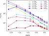 |
Fig. 5 12C/13C ratio in the LIMS models of Cristallo et al. (2009, 2011, 2015) as a function of metallicity, for different non-rotating stellar masses. |
5.2 Chemical evolution of the 12C/13C ratio
We present here the results of the chemical evolution model for the 12C/13C ratio, using the yields and assumptions described in Section 4. In particular, we recall that massive stars rotate at 150 km s−1 above [Fe/H] > −3 and 300 km s−1 below [Fe/H] ≤ −3, with the yields from Limongi & Chieffi (2018) for [Fe/H] ≥ −3 and from Roberti et al. (2024) for [Fe/H] < −3.
The model outcome is presented in Fig. 6. The behaviour of the model can be easily interpreted in light of the stellar yields we discussed above. Below [Fe/H] < −4, the model is dominated by the zero-metal massive stars: two long tracks extend towards the lowest metallicity, corresponding to the two zero-metal rotating models of 15 and 25 M⊙, plus their interpolation (no extrapolation is used, see Section 4). Although the grid of yields is incomplete, we can see that the model is able to reproduce the observations at [Fe/H] < −4 thanks to the presence of 25 M⊙ stars with predicted 12C/13C = 56 due to shell merging. The model also extends towards much higher 12C/13C, because Article number, page 8 of 16 the other stars produce small 13C and large 12C/13C > 103 due to their lack of shell merging.
Going towards [Fe/H] > −4 the model rises sharply above 12C/13C > 103, because the yields for massive stars by Limongi & Chieffi (2018) predict large 12C/13C especially in the range −3 < [Fe/H] < −2. From [Fe/H] > −2.5 the model starts decreasing again due to the contribution from AGB stars. As we showed in Fig. 5, this is due to the first 3–6 M⊙ stars that die from around 60 Myr and [Fe/H] = −3, enriching the ISM of a 12C/13C ratio below 300 due to hot bottom burning, strongly bringing down the ratio that was around ~103 due to massive stars. We confirm the contribution from massive AGB stars from the age-metallicity relation that we include in the appendix (Fig. B.1).
From around [Fe/H] > −1.5 also the lower-mass stars begin to die, and their 12C/13C is high, so the model starts rising again. Nevertheless, we recognise that the scenario above [Fe/H] > −2 is really complex, due to the different contributions from both low-mass and massive stars, while observations in this range are scarce and uncertain. Since we cannot use observations to constrain the producers of 13C, we prefer not to draw conclusions for this metallicity range. The solar value is 12C/13C = 91 ± 1.3 (Goto et al. 2003; Ayres et al. 2013), however, we recall that the version of the GEMS code we use here is for simulating the halo, therefore we do not expect the model to reproduce the solar value.
Finally, we notice that the model cannot reproduce the observations below 12C/13C < 30 (indicated by a dashed line in Fig. 6). No stellar yield adopted in this study can produce enough 13C to reach such a low ratio. Although explaining the composition of these stars is difficult and still a matter of debate, there are possible explanations that involve the physics of the producers or of the host stars. We comment on this point later in Sect. 5.3.
In order to evaluate the impact of the H-He shell mergers on the chemical evolution, also in relation to the observations, we present in Fig. 7 the same chemical evolution model, but assuming that all stars in the range 20–25 M⊙ at [Fe/H] ≤ −3 present a H-He shell merger. Since there are still not enough stellar models available, we used the yields for 12C and 13C from the zero-metal 25 M⊙ stellar model with vini = 300 km s−1 from Roberti et al. (2024). The model in Fig. 7 predicts a much smaller 12C/13C ratio at low metallicity, with most points between 50–300, much more in line with the observations that are all below 12C/13C < 100. These results show that a more frequent occurrence of shell mergers is preferable at low metallicity. This model still cannot reproduce the data below 12C/13C < 30, since we did not allow for extrapolation outside the stellar model predictions.
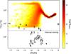 |
Fig. 6 Isotopic ratio 12C/13C versus [Fe/H]. The stochastic model is the colour map, with the number of simulated stars on a logarithmic scale. The dots are the observed halo stars (dwarfs in black, giants in white) as presented in Molaro et al. (2023), complete of their possible error. The horizontal line 12C/13C = 30 marks the evidence for internal mixing in giant stars (Spite et al. 2006). |
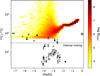 |
Fig. 7 Same as Fig. 6, but for a model with H-He shell mergers in all 20 to 25 M⊙ stars at [Fe/H] ≤ −3. |
5.3 Explanations for the low 12C/13C ratio
We have seen that many observations of halo stars have a 12C/13C ratio that lies below 30 (see Fig. 6 and Molaro et al. 2023). Stars in this region cannot be explained by the usual nucleosynthesis sites, therefore alternative physical mechanisms are required to explain their low 12C/13C. Possible explanations involve modifications in the production sites, or in the surface abundances of the host stars, or a combination of both. Spite et al. (2006) have studied a sample of extremely metal poor RGB stars, finding evidence for modified surface abundances due to interior processes. A group of giants on the lower red giant branch, therefore less evolved (’unmixed giants’), showed a 12C/13C ratio around 30 (see also Spite et al. 2021), which therefore is sometimes described as the unmixed limit. Recently, stellar modelling has been investigating the possible depletion mechanisms in giant stars, through detailed comparison with individual observations. Marini et al. (2023), using the ATON code, showed that 2.5–2.7 M⊙ stars at solar metallicity display an important decrease in 12C/13C surface abundance from about 90 to 20, only due to the first dredge-up during the RGB phase. Additionally, Mohorian et al. (2024) and Nguyen et al. (2025) found independently, the former employing the ATON and the latter the PARSEC code, that for stars ≤1 M⊙ with metallicity from solar down to Z = 10−4 (around [Fe/H] = −2.6 in our galactic model), the initial 12C/13C = 90 can be depleted to less than 10 due to the combined effects of thermohaline mixing and envelope overshooting. However, all these studies assume the solar ratio as the initial value, while at lower metallicity the initial surface ratio could be higher (see Fig. 6), therefore we cannot reconstruct the original surface abundance of giants in our range of interest.
In the sample we use here, 6 stars with 12C/13C < 30 are not giants (see Section 2 and Fig. 6). They should therefore retain their original surface 12C/13C. A possible explanation for their low ratio is that the H-He shell mergers we explore in this study are able to produce much lower 12C/13C. Choplin et al. (2016) showed that an equilibrium value of ~4 can be obtained in a one-zone nuclear model of CNO burning with mixing between H and He. Choplin et al. (2017) implemented this in stellar models and were able to obtain yields of 12C/13C ~ 4 in massive-star outer layers by triggering a late H-He mixing event, at metallicity [Fe/H] = −3.8 with very fast rotation (vini = 600–700 km s−1). Clarkson & Herwig (2021) also found very low ratios 12C/13C ≳ 1.5 in outer layers of zero-metal massive-star models without rotation. Considering the extra energy released by the proton ingestion, it is possible that the merging event produces enough energy to expel the outer layers before the SN explosion. However, a contribution by only outer layers, without deep layer ejection, would not be able to explain the observations. Iron is needed, from the inner layers of the same or other stars, to explain the [Fe/H] measurements. But if iron is ejected, so it is the abundant 12C in the inner layers, and 12C/13C increases.
We show in Fig. 8 the stochastic model when 20–25 M⊙ stars at [Fe/H] ≤ −3, the ones we assume produce shell mergers, only eject their outer regions. We used the yields from the same stellar models, but placed a mass cut at the base of the shell merger; this allowed to eject the equilibrium 12C/13C ~ 4 in the shell, but no iron. Stars < 20 M⊙ still undergo full SN explosion and eject Fe and 12C. Therefore, stars at [Fe/H] < −3 form from a mixture of progenitors with 12C/13C ~ 4 but no iron or with large 12C/13C and iron. The bulk of the model sits at 12C/13C > 20 because the low 12C/13C in the outer layer ejecta is mixed with the 12C-rich deep ejecta, increasing the ratio. A low probability region 12C/13C < 20 is the result of volumes with many more progenitors 20–25 M⊙ than 8–15 M⊙, which is disfavoured but not unviable. As metallicity increases, more 12C accumulates in the ISM and the 12C/13C ratio keeps increasing. These assumptions cannot reproduce the observations of our 6 dwarf stars at 12C/13C < 15, which remain completely outside the model.
The only way of explaining all 12C/13C < 30 with massive stars is to assume a larger production of 12C and 13C from H-He shell mergers, which can be obtained either increasing the yields of massive stars or their number. As an example of the possible impact, we show in Fig. 9 the same chemical evolution model of Fig. 8, with shell mergers and outer layer ejection from 20–25 M⊙ stars at [Fe/H] ≤ −3, but assuming a production of 12C and 13C that is 10 times larger than what predicted by the models of Roberti et al. (2024). This is a tentative approach since such a large production is not based on any stellar model; however, this assumption pushes the 12C/13C ratio to very low values that can be more in agreement with the observations. Similar results can be obtained assuming that more stars ≥20 M⊙ can form compared to lower ones, therefore modifying the IMF. Evidences show that the IMF is possibly biased towards more massive stars at lower metallicity (Schneider et al. 2018; Zhang et al. 2018).
However, only changing the IMF would not be enough to have the larger production of 13C required to lower the 12C/13C ratio. To show this, we recomputed some of the models presented above employing the IMF from Kroupa (2001), which is more top-heavy compared to the one by Scalo (1986); the models are shown in the appendix (Figs. C.1 and C.2). The impact of the IMF is not significant: in particular, the bulk of the models, i.e. where the density of stars is larger, slightly shifts towards lower 12C/13C, but the nucleosynthesis sources are the same as before and the IMF has not a strong enough effect on the number of massive stars to consistently lower 12C/13C. Tests run with even more top-heavy IMF (Schneider et al. 2018) produce the same results.
Alternatively, it is possible to have a different threshold for the failed explosion or for the outer layer ejection. Indeed, the question of explodability for core-collapse supernovae in stars of different mass is still uncertain (Burrows & Vartanyan 2021; Boccioli et al. 2023). Unfortunately, the grid of Roberti et al. (2024) only encompasses two masses, so we cannot predict yet the effects of shell mergers in stars of different mass. In the grid of Limongi & Chieffi (2018) (see Fig. 2), there is a general trend of increasing 12C/13C with larger mass, so a lower threshold for the failed explosion would decrease 12C/13C. On the other hand, if higher-mass stars >25 M⊙ also produce shell mergers and only eject their outer layers, a wider mass range for outer layer ejection would be beneficial and lower 12C/13C, since these stars could have an even larger production of 13C, given their mass, without ejecting the internal matter rich in 12C. Nevertheless, in order to shed more light on these issues additional stellar models of massive stars at low metallicity need to be produced.
Finally, we notice that assuming only outer layer ejection, the 12C/13C remains low and cannot reproduce anymore the observations at [Fe/H] < −4.5, which have 12C/13C > 30. Shell mergers followed by complete supernova explosions were instead effective in explaining them, as we discussed in the previous Section. Therefore, it appears that both complete and incomplete ejection of material from stars with shell mergers are required to explain the entire range of 12C/13C observed.
It is worth mentioning here that the assumption of outer layer ejection does not change significantly the chemical evolution of the other elements. CNO are still abundantly produced by lower mass stars and H-He shell mergers. Heavy elements are not produced in zero-metal stars in the first place, due to the lack of seed nuclei for neutron capture (see Roberti et al. 2024).
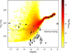 |
Fig. 8 Same as Fig. 7, but assuming that 20–25 M⊙ stars at [Fe/H] ≤ −3 only eject the outer layers at the end of their lives. |
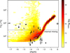 |
Fig. 9 Same as Fig. 8, but assuming that H-He shell mergers in 20–25 M⊙ stars at [Fe/H] ≤ −3 produce 10 times more 12C and 13C in the ejected outer layers than what currently predicted. |
5.4 Chemical evolution of the CNO elements
In Fig. 10, we present the predicted ratios [C/Fe], [N/Fe], and [O/Fe] for the model presented in Section 5.2, Fig. 6 together with the observations of dwarf stars or unmixed giants (see Section 2). These results are not significantly different from the other models with modified ejecta (see Sections 5.2 and 5.3). Towards the lowest metallicity, the model predicts a long and narrow tail reaching very high values, due to the production from massive stars that eject mainly constant CNO and very little iron. Not many observations exist in this range except for carbon: the observed [C/Fe] always lie higher than the model for [Fe/H] ≲ −4. This was also found by Cescutti et al. (2016) assuming the rotating yields of Meynet & Maeder (2002) and Hirschi (2007). It could be due to the yields for massive stars underestimating C production, but also due to 1D LTE assumptions in the observations. In fact, 3D and NLTE corrections show a lower [C/Fe] measured at low metallicity (Lind & Amarsi 2024), down to ~1 dex. For metallicity −4 < [Fe/H] < −2, the model is able to reproduce the normal stars, but not the CEMP stars ([C/Fe] > 1). The same result was found in the similar work of Cescutti & Chiappini (2010). Some of these stars have a very high C/H ratio, comparable to that of CEMP-s stars; they are sometimes called ‘super-CEMP’ stars (Cooke & Madau 2014). Possible explanations for their high C involve binary interaction (Starkenburg et al. 2014; Arentsen et al. 2019), or an ISM that was not well mixed (Bonifacio et al. 2003; Chieffi & Limongi 2003; Meynet et al. 2010), or internal mixing (Maeder & Meynet 2015). Consequently, if on one hand zero-metal rotating massive stars with shell mergers can explain the 12C/13C ratio, on the other hand, the [C/Fe] ratio is underestimated at the same metallicity. We interpret this result in the following way. In the stellar models of Roberti et al. (2024), the carbon yields generally increase with stellar rotation, both in the 15 and 25 M⊙ models, up to around a factor of 2. Therefore, the [C/Fe] observations can be explained assuming that primordial massive stars had even higher rotation velocity (Roberti et al. 2024 have run tests up to almost critical velocity), while the 12C/13C observed in the same stars can be explained through shell merging events. The only way to combine both scenarios is to assume that H-He shell mergers are more common than what is currently found in stellar models, at least for extremely low metallicity. Roberti et al. (2024) found that rotation seems to disfavour H-He shell mergers; however, recent findings from 3D stellar models (Mocák et al. 2018; Yadav et al. 2020; Rizzuti et al. 2024) seem to indicate that shell mergers may be more frequent once multi-dimensionality is taken into account.
For [Fe/H] > −2, the contribution from LIMS becomes important, so we do not extrapolate results from the model in this range. The picture is complicated by the fact that these elements are produced by both massive and low-mass stars, therefore a combination of the two is required to explain the observations in this metallicity range. This is beyond the scope of this work.
Figure 11 shows the ratios in the form of log(C/O) and log(N/O) versus log(O/H)+12. In this way, the dependence from iron is removed and the elements are only studied in relation to each other. From the C/O ratio, we can see that the model is in line with the observations at lower metallicity, but is clearly overestimated at higher ones; this comes from the fact that the yields for carbon in set R by Limongi & Chieffi (2018) are generally overestimated compared to oxygen at [Fe/H] > −2 (see Fig. 10), as also pointed out by Prantzos et al. (2018); Romano et al. (2019); Kobayashi (2022). From the C/O plot, we also notice that both model and observational trends are very narrow, because carbon and oxygen are produced in the same way. This is not the case for N/O, which instead presents a large spread at low metallicity both in the model and in the data. This can be explained considering that N has a primary production in rotating massive stars, being highly dependent on the stellar rotation, and the fact that massive stars above 25 M⊙ contribute only through stellar wind, enriching the ISM with high N/O that is then diluted with material from stars <25 M⊙ (see also Cescutti & Chiappini 2010). The stochastic model can reproduce most of this spread. Going towards higher metallicity, the N/O trend follows the one of the observations, although not perfectly since we did not calibrate the model for these metallicities.
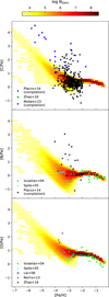 |
Fig. 10 [C/Fe], [N/Fe], and [O/Fe] versus [Fe/H]. The stochastic model is the colour map, with the number of simulated stars in log scale. The dots are the observed dwarf or unmixed giant halo stars as presented in Section 2. |
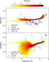 |
Fig. 11 log(C/O) and log(N/O) versus log(O/H)+12. The stochastic model is the colour map, with the number of simulated stars in log scale. The dots are the observed dwarf or unmixed giant halo stars as presented in Section 2. The symbol of the Sun refers to solar values (Asplund et al. 2009). |
5.5 Chemical evolution of Sr and Ba
In Fig. 12, we show the predicted ratios [Sr/Fe], [Ba/Fe] and [Sr/Ba] from the same model compared to the observations. We remind that s-process material can be produced in rotating massive stars thanks to the rotation-induced mixing that stirs material between the H- and He-burning regions, enhancing the nucleosynthesis and neutron-capture thanks to the production of 14N and its conversion to 22Ne as neutron source (see Limongi & Chieffi 2018). These effects are even more important at low metallicity, where stars are more compact and tend to rotate faster, and where the neutron-to-seed ratio drastically increases, favouring the production of heavier nuclei (see the discussion on s-process in Gallino et al. 1998). This is of crucial importance, as massive stars are thought to only contribute to the weak s-process component (Sr–Y–Zr). In this way, they can also contribute to the main component (Ba-La-Ce), but not to the heavy one (Pb). Although zero-metal stars cannot synthesise s-process elements due to their lack of iron seeds for neutron capture, already the next generation of stars ([Fe/H] = −5 in our model) begins the production (see Roberti et al. 2024).
The stochastic model is able to reproduce the majority of the observations, even at extremely low metallicity. The long horizontal lines in [Sr/Ba] towards low metallicity come from the fact that few masses are present in the grid of yields below [Fe/H] < −3. It is meaningful here to make a comparison between these results and the ones presented in Rizzuti et al. (2021) for the same abundance ratios. The model of Rizzuti et al. (2021) is able to better reproduce the trend and spread of Sr and Ba in the observations, thanks to the fact that they calibrated the massive-star rotation velocity, while here we use a simplified distribution. Above [Fe/H] > −2, the model is less accurate, because it has not been calibrated for this metallicity range, and the impact from AGB stars begins to be important. The new data from François et al. (2024) show an important increase in Ba at higher metallicity compared to the model predictions: this is an interesting point that will require additional investigation in the future.
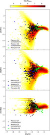 |
Fig. 12 [Sr/Fe], [Ba/Fe], and [Sr/Ba] versus [Fe/H]. The stochastic model is the colour map, with the number of simulated stars in log scale. The dots are the observed halo stars as presented in Section 2. |
6 Conclusions
In this paper, we investigate the production of light elements C, N, O, and the 12C/13C ratio in zero-metal and extremely-low-metallicity stars. This has been required by the recent observation campaigns of stars in the Galactic halo. Explaining these 12C/13C ratios at low metallicity is challenging, considering that the measurements span the range of 3 < 12C/13C < 100, requiring a consistent production of 13C that must be primary.
This production of 13C is expected to come from massive stars, which are the main contributors at these low metallicities. Over the years, stellar modelling studies have shown that 13C can be produced in a primary fashion via an interaction between H and He shells, assuming a mixing between these layers that can be favoured by rotation (Hirschi 2007; Choplin et al. 2017; Limongi & Chieffi 2018; Tsiatsiou et al. 2024) or convection (Limongi & Chieffi 2012; Clarkson & Herwig 2021), or a combination of both (Roberti et al. 2024). However, it is presently believed that stars at low metallicity need to be fast rotators, for reasons that are related to both the physics involved (Meynet & Maeder 2002) and nucleosynthesis (Chiappini et al. 2006; Cescutti et al. 2013).
In this study, we have employed the GEMS chemical evolution model, the latest version of the stochastic model by Cescutti & Chiappini (2010). The model includes the most up-to-date nucleosynthesis sources available in the literature, including the recent work by Roberti et al. (2024), which presents stellar evolution models for zero-metal and low-metallicity rotating massive stars. We found no need to include the contribution from very massive (>100 M⊙) and supermassive (>1000 M⊙) Pop III stars, and we generally treated Pop III stars as if they have no qualitative difference from low-metallicity stars, except in terms of the differences in metal content. We show that thanks to the H-He shell merging event occurring in some massive stars, the chemical evolution model is able to reproduce the observations at 12C/13C > 30. The model is in best agreement with the observations if we assume that H-He shell mergers occur in all 20–25 M⊙ stars at [Fe/H] ≤ −3. The evolution of [CNO/Fe] can also be adequately reproduced for low-metallicity stars except for CEMP and super-CEMP stars. The discrepancy with the observations at the lowest metallicity in [C/Fe] and C/O can be attributed to 3D and NLTE effects in the measurements (Lind & Amarsi 2024). Additionally, we reproduced the evolution of heavy elements Sr and Ba, generated in part by the same sources, but not calibrated in this work.
Explaining the observations below 12C/13C < 30 still remains an open question. Different stellar modelling studies have been showing that a very low 12C/13C ratio can be obtained in stellar winds or outer layers of massive stars (e.g. Hirschi 2007; Choplin et al. 2017; Clarkson & Herwig 2021). The ejection of only the outer layers can be caused by the energy produced at the base of the shell merger (see Clarkson & Herwig 2021), followed by a collapse of the star with no SN explosion. However, to reproduce at the same time both the 12C/13C and [Fe/H] measured in CEMP stars, it is necessary to assume that they formed from both inner and outer layers of SN ejections, from the same or different stars.
We have shown here that observations at 12C/13C < 30 can be explained assuming that the 13C-rich outer layers are expelled from the star with no subsequent SN explosion, then mixed with Fe from other SN remnants, but only if the production of 13C is ten times larger than what currently predicted – which is at best ~10−2 M⊙ in 20–25 M⊙ stars with shell mergers. This cannot be achieved only assuming that the number of massive stars is larger than what is currently assumed, although observational evidence pointed out that the IMF could be biased towards more massive stars at lower metallicity (Schneider et al. 2018; Zhang et al. 2018; Rossi et al. 2021). Another possibility is that also stars >25 M⊙ produce H-He shell mergers and eject them before their final collapse, given that the energy released from the merging is enough to eject the outer layers. Although these stars are fewer in number, their higher mass could contribute to a larger production of 13C.
However, to keep reproducing also the 12C/13C > 30 observations at lowest metallicity, it is necessary to assume that some stars also formed from complete SN ejecta. This is possible either if it is present a threshold around the mass range of 20–25 M⊙ that separates complete and incomplete ejection, or if the ejection occurs differently in stars with the same mass, depending on physical properties such as rotation or magnetic fields (see Varma et al. 2023; Boccioli & Roberti 2024). Therefore, we have made a distinction between faint and failed supernovae: the former still eject small quantities of iron, necessary to explain the [Fe/H] measured in CEMP stars; the latter need to eject only the outer layers, enriching the ISM of low 12C/13C material.
Overall, the work we presented here shows the need for H-He shell mergers to explain the nucleosynthesis of the first stars. The occurrence of H-He interacting shells has been reported on in stellar modelling both for zero-metal (Woosley & Weaver 1982; Heger & Woosley 2010; Limongi & Chieffi 2012; Clarkson & Herwig 2021) and low-metallicity (Hirschi 2007; Choplin et al. 2017; Ritter et al. 2018) stars. It is important to underline that they are expected to be more frequent at lower metallicity, due to the lower opacity of the star, lower entropy jump, and smaller distance between the shells both in radius and in mass. Roberti et al. (2024) concluded that stellar rotation seems to disfavour the occurrence of H-He shell mergers. However, these occurrences are strongly dependent on the convective and overshoot prescriptions used in the stellar models.
Recent findings from both 1D and 3D stellar models seem to indicate that the mixing-length-theory (Böhm-Vitense 1958) normally used to reproduce convection may be inaccurate for advanced phases of massive stars (Arnett et al. 2018; Rizzuti et al. 2022; Georgy et al. 2024) and H–He interacting environments (Herwig et al. 2011, 2014; Jones et al. 2016). Convective-boundary-mixing (overshoot) prescriptions also appear to be equally underestimated (Scott et al. 2021; Cristini et al. 2019; Rizzuti et al. 2023). While 3D simulations of H-ingestion environments have only been focusing on AGB stars (Mocák et al. 2011; Stancliffe et al. 2011; Herwig et al. 2014), late-type C–Ne–O shell mergers have already been confirmed to occur also in 3D stellar models (Yadav et al. 2020; Rizzuti et al. 2024). The implementation of stronger convection in the stellar models would naturally result in more frequent occurrence of shell mergers.
It is clear that to shed more light on these issues, additional stellar models of zero-metal and low-metallicity rotating massive stars are necessary. This is especially important for modelling the Galactic chemical evolution, which is largely based on detailed grids of the stellar yields. Even though many uncertainties remain with respect to the specific parameters used in stellar models, results from Galactic archaeology can provide useful constraints on the physics of stars. These include their mass distribution, rotation velocity, frequency of ingestion events, and respective fates. Therefore, having better constraints on the nucleosynthesis of the first stars will also have important implications for our knowledge of their physics, which remains largely obscure today.
Acknowledgements
FR, GC, and LM acknowledge financial support under the National Recovery and Resilience Plan (NRRP), Mission 4, Component 2, Investment 1.1, Call for tender No. 104 published on 2.2.2022 by the Italian Ministry of University and Research (MUR), funded by the European Union – NextGenerationEU – Project ‘Cosmic POT’ (PI: L. Magrini) Grant Assignment Decree No. 2022X4TM3H by the Italian Ministry of Ministry of University and Research (MUR). GC and LM thank INAF for the support (Large Grant 2023 EPOCH) and for the MiniGrant 2022 Checs. LR acknowledges the support from the NKFI via K-project 138031 and the Lendület Program LP2023-10 of the Hungarian Academy of Sciences. This work has been partially supported by the Italian grants “Premiale 2015 FIGARO” (PI: Gianluca Gemme). We acknowledge support from PRIN MUR 2022 (20224MNC5A), “Life, death and after-death of massive stars”, funded by European Union – Next Generation EU. FM thanks INAF for the 1.05.12.06.05 Theory Grant – Galactic archaeology with radioactive and stable nuclei. FM acknowledges also support from Project PRIN MUR 2022 (code 2022ARWP9C) “Early Formation and Evolution of Bulge and HalO (EFEBHO)” (PI: M. Marconi). This work was also partially supported by the European Union (ChETEC-INFRA, project no. 101008324).
Appendix A Kiel diagram of the observations
Evolutionary effects during the lifetime of observed stars could modify the original surface abundances of light elements. In order to compare the chemical evolution models to original surface abundances, we made a selection on the observations (see Section 2). We present in Fig. A.1 the log(g) versus Teff of all the stars considered in this work. We compare them to isochrones obtained from PARSEC models (Bressan et al. 2012; Chen et al. 2014; Fu et al. 2018) for ages of 12 Gyr and metallicity between −2.4 < [Fe/H] < −1.2; unfortunately, no lower metallicity is available. Most stars have been selected to be dwarfs with log(g) ≥ 3.2, to avoid internal mixing effects. The only stars with log(g) < 3.2 are from Spite et al. (2005) who used Li to select unmixed giants, François et al. (2024) from which we only used Sr and Ba abundances, and Molaro et al. (2023) where we make a distinction between dwarfs and giants when comparing to the models.
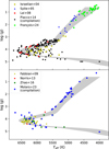 |
Fig. A.1 Kiel diagram (log(g) versus Teff) for the observations presented in Section 2. The shaded areas are 12 Gyr isochrones obtained from PARSEC models, with metallicity between [Fe/H] = −2.4 (Z = 0.0001) and [Fe/H] = −1.2 (Z = 0.0015). |
Appendix B Age-metallicity relation
To demonstrate the impact of stars of different mass on the nucleosynthesis, we display in Fig. B.1 the relation between [Fe/H] and time in our stochastic simulation. The dispersion is very narrow and the trend is monotonically increasing. In particular, we notice that the first massive AGB stars ≲ 6 M⊙ that die after ≳ 60 Myr are only in large enough number to be impactful after [Fe/H] > −3, and cannot die before [Fe/H] = −5.
 |
Fig. B.1 Age-metallicity relation ([Fe/H] versus time) in the stochastic model of Fig. 6 shown as a colour map. |
Appendix C Changing the initial mass function
The choice of a different initial mass function can potentially have an impact on the number and frequency of H-He shell mergers. We show in Fig. C.1 and C.2 the chemical evolution models from Fig. 6 and 8, respectively, recomputed with the IMF from Kroupa (2001) instead of the one by Scalo (1986). Comparing the models with different IMF, it is possible to see that its impact is not significant: the models are slightly shifted towards higher [Fe/H], and at high metallicity 12C/13C is larger due to more 12C and no 13C coming from massive stars at intermediate metallicity. There is indeed a larger density of stars with lower 12C/13C, but the model cannot extend further since the nucleosynthesis sources are the same as before, and the IMF has not a strong enough effect on their number.
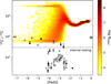 |
Fig. C.1 Same model as in Fig. 6 (shell mergers with yields of Roberti et al. 2024), but assuming an IMF from Kroupa (2001) instead of Scalo (1986). |
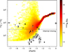 |
Fig. C.2 Same model as in Fig. 8 (shell mergers and outer layer ejection in 20 - 25 M⊙ stars at [Fe/H] ≤ −3), but assuming an IMF from Kroupa (2001) instead of Scalo (1986). |
References
- Aguado, D. S., González Hernández, J. I., Allende Prieto, C., & Rebolo, R. 2018, ApJ, 852, L20 [NASA ADS] [CrossRef] [Google Scholar]
- Aguado, D. S., González Hernández, J. I., Allende Prieto, C., & Rebolo, R. 2019, ApJ, 874, L21 [NASA ADS] [CrossRef] [Google Scholar]
- Aguado, D. S., Molaro, P., Caffau, E., et al. 2022, A&A, 668, A86 [NASA ADS] [CrossRef] [EDP Sciences] [Google Scholar]
- Aguado, D. S., Caffau, E., Molaro, P., et al. 2023, A&A, 669, L4 [NASA ADS] [CrossRef] [EDP Sciences] [Google Scholar]
- Allen, D. M., Ryan, S. G., Rossi, S., Beers, T. C., & Tsangarides, S. A. 2012, A&A, 548, A34 [NASA ADS] [CrossRef] [EDP Sciences] [Google Scholar]
- Aoki, W., Norris, J. E., Ryan, S. G., Beers, T. C., & Ando, H. 2002, ApJ, 567, 1166 [Google Scholar]
- Arentsen, A., Starkenburg, E., Shetrone, M. D., et al. 2019, A&A, 621, A108 [NASA ADS] [CrossRef] [EDP Sciences] [Google Scholar]
- Argast, D., Samland, M., Thielemann, F. K., & Gerhard, O. E. 2002, A&A, 388, 842 [NASA ADS] [CrossRef] [EDP Sciences] [Google Scholar]
- Argast, D., Samland, M., Thielemann, F. K., & Qian, Y. Z. 2004, A&A, 416, 997 [NASA ADS] [CrossRef] [EDP Sciences] [Google Scholar]
- Arnett, W. D., Hirschi, R., Campbell, S. W., et al. 2018, preprint [Google Scholar]
- Asplund, M., Grevesse, N., Sauval, A. J., & Scott, P. 2009, ARA&A, 47, 481 [NASA ADS] [CrossRef] [Google Scholar]
- Ayres, T. R., Lyons, J. R., Ludwig, H. G., Caffau, E., & Wedemeyer-Böhm, S. 2013, ApJ, 765, 46 [NASA ADS] [CrossRef] [Google Scholar]
- Beers, T. C., Preston, G. W., & Shectman, S. A. 1985, AJ, 90, 2089 [NASA ADS] [CrossRef] [Google Scholar]
- Beers, T. C., Preston, G. W., & Shectman, S. A. 1992, AJ, 103, 1987 [NASA ADS] [CrossRef] [Google Scholar]
- Bessell, M. S., & Norris, J. 1984, ApJ, 285, 622 [NASA ADS] [CrossRef] [Google Scholar]
- Boccioli, L., & Roberti, L. 2024, Universe, 10, 148 [NASA ADS] [CrossRef] [Google Scholar]
- Boccioli, L., Roberti, L., Limongi, M., Mathews, G. J., & Chieffi, A. 2023, ApJ, 949, 17 [CrossRef] [Google Scholar]
- Böhm-Vitense, E. 1958, ZAp, 46, 108 [NASA ADS] [Google Scholar]
- Bonifacio, P., Molaro, P., Beers, T. C., & Vladilo, G. 1998, A&A, 332, 672 [NASA ADS] [Google Scholar]
- Bonifacio, P., Limongi, M., & Chieffi, A. 2003, Nature, 422, 834 [CrossRef] [Google Scholar]
- Bonifacio, P., Caffau, E., Spite, M., et al. 2015, A&A, 579, A28 [NASA ADS] [CrossRef] [EDP Sciences] [Google Scholar]
- Bonifacio, P., Caffau, E., Spite, M., et al. 2018, A&A, 612, A65 [NASA ADS] [CrossRef] [EDP Sciences] [Google Scholar]
- Bressan, A., Marigo, P., Girardi, L., et al. 2012, MNRAS, 427, 127 [NASA ADS] [CrossRef] [Google Scholar]
- Burrows, A., & Vartanyan, D. 2021, Nature, 589, 29 [CrossRef] [PubMed] [Google Scholar]
- Busso, M., Gallino, R., & Wasserburg, G. J. 1999, ARA&A, 37, 239 [Google Scholar]
- Caffau, E., Bonifacio, P., Sbordone, L., et al. 2013, A&A, 560, A71 [NASA ADS] [CrossRef] [EDP Sciences] [Google Scholar]
- Caffau, E., Bonifacio, P., Spite, M., et al. 2016, A&A, 595, L6 [NASA ADS] [CrossRef] [EDP Sciences] [Google Scholar]
- Cavallo, L., Cescutti, G., & Matteucci, F. 2021, MNRAS, 503, 1 [CrossRef] [Google Scholar]
- Cescutti, G. 2008, A&A, 481, 691 [NASA ADS] [CrossRef] [EDP Sciences] [Google Scholar]
- Cescutti, G., & Chiappini, C. 2010, A&A, 515, A102 [NASA ADS] [CrossRef] [EDP Sciences] [Google Scholar]
- Cescutti, G., & Chiappini, C. 2014, A&A, 565, A51 [NASA ADS] [CrossRef] [EDP Sciences] [Google Scholar]
- Cescutti, G., Chiappini, C., Hirschi, R., Meynet, G., & Frischknecht, U. 2013, A&A, 553, A51 [NASA ADS] [CrossRef] [EDP Sciences] [Google Scholar]
- Cescutti, G., Romano, D., Matteucci, F., Chiappini, C., & Hirschi, R. 2015, A&A, 577, A139 [NASA ADS] [CrossRef] [EDP Sciences] [Google Scholar]
- Cescutti, G., Valentini, M., François, P., et al. 2016, A&A, 595, A91 [NASA ADS] [CrossRef] [EDP Sciences] [Google Scholar]
- Cescutti, G., Bonifacio, P., Caffau, E., et al. 2022, A&A, 668, A168 [NASA ADS] [CrossRef] [EDP Sciences] [Google Scholar]
- Chamberlain, J. W., & Aller, L. H. 1951, ApJ, 114, 52 [NASA ADS] [CrossRef] [Google Scholar]
- Chen, Y., Girardi, L., Bressan, A., et al. 2014, MNRAS, 444, 2525 [Google Scholar]
- Chiappini, C., Hirschi, R., Meynet, G., et al. 2006, A&A, 449, L27 [NASA ADS] [CrossRef] [EDP Sciences] [Google Scholar]
- Chiappini, C., Ekström, S., Meynet, G., et al. 2008, A&A, 479, L9 [NASA ADS] [CrossRef] [EDP Sciences] [Google Scholar]
- Chieffi, A., & Limongi, M. 2003, PASA, 20, 324 [Google Scholar]
- Chieffi, A., & Limongi, M. 2013, ApJ, 764, 21 [Google Scholar]
- Chieffi, A., & Limongi, M. 2020, ApJ, 890, 43 [NASA ADS] [CrossRef] [Google Scholar]
- Choplin, A., Maeder, A., Meynet, G., & Chiappini, C. 2016, A&A, 593, A36 [NASA ADS] [CrossRef] [EDP Sciences] [Google Scholar]
- Choplin, A., Ekström, S., Meynet, G., et al. 2017, A&A, 605, A63 [NASA ADS] [CrossRef] [EDP Sciences] [Google Scholar]
- Clarkson, O., & Herwig, F. 2021, MNRAS, 500, 2685 [Google Scholar]
- Cohen, J. G., Christlieb, N., McWilliam, A., et al. 2004, ApJ, 612, 1107 [CrossRef] [Google Scholar]
- Collins, C., Müller, B., & Heger, A. 2018, MNRAS, 473, 1695 [NASA ADS] [Google Scholar]
- Cooke, R. J., & Madau, P. 2014, ApJ, 791, 116 [Google Scholar]
- Cristallo, S., Straniero, O., Gallino, R., et al. 2009, ApJ, 696, 797 [NASA ADS] [CrossRef] [Google Scholar]
- Cristallo, S., Piersanti, L., Straniero, O., et al. 2011, ApJS, 197, 17 [NASA ADS] [CrossRef] [Google Scholar]
- Cristallo, S., Straniero, O., Piersanti, L., & Gobrecht, D. 2015, ApJS, 219, 40 [Google Scholar]
- Cristini, A., Hirschi, R., Meakin, C., et al. 2019, MNRAS, 484, 4645 [NASA ADS] [CrossRef] [Google Scholar]
- Curtis, S., Ebinger, K., Fröhlich, C., et al. 2019, ApJ, 870, 2 [Google Scholar]
- Deng, L.-C., Newberg, H. J., Liu, C., et al. 2012, Res. Astron. Astrophys., 12, 735 [Google Scholar]
- Ekström, S., Meynet, G., Chiappini, C., Hirschi, R., & Maeder, A. 2008, A&A, 489, 685 [NASA ADS] [CrossRef] [EDP Sciences] [Google Scholar]
- Fabbian, D., Nissen, P. E., Asplund, M., Pettini, M., & Akerman, C. 2009, A&A, 500, 1143 [NASA ADS] [CrossRef] [EDP Sciences] [Google Scholar]
- François, P., Cescutti, G., Bonifacio, P., et al. 2024, A&A, 686, A295 [NASA ADS] [CrossRef] [EDP Sciences] [Google Scholar]
- Frebel, A., Chiti, A., Ji, A. P., Jacobson, H. R., & Placco, V. M. 2015, ApJ, 810, L27 [NASA ADS] [CrossRef] [Google Scholar]
- Frebel, A., Ji, A. P., Ezzeddine, R., et al. 2019, ApJ, 871, 146 [NASA ADS] [CrossRef] [Google Scholar]
- Frischknecht, U., Hirschi, R., & Thielemann, F. K. 2012, A&A, 538, L2 [NASA ADS] [CrossRef] [EDP Sciences] [Google Scholar]
- Frischknecht, U., Hirschi, R., Pignatari, M., et al. 2016, MNRAS, 456, 1803 [Google Scholar]
- Fu, X., Bressan, A., Marigo, P., et al. 2018, MNRAS, 476, 496 [NASA ADS] [CrossRef] [Google Scholar]
- Gallino, R., Arlandini, C., Busso, M., et al. 1998, ApJ, 497, 388 [Google Scholar]
- Georgy, C., Rizzuti, F., Hirschi, R., et al. 2024, MNRAS, 531, 4293 [Google Scholar]
- González Hernández, J. I., Aguado, D. S., Allende Prieto, C., Burgasser, A. J., & Rebolo, R. 2020, ApJ, 889, L13 [CrossRef] [Google Scholar]
- Goto, M., Usuda, T., Takato, N., et al. 2003, ApJ, 598, 1038 [NASA ADS] [CrossRef] [Google Scholar]
- Grisoni, V., Romano, D., Spitoni, E., et al. 2020, MNRAS, 498, 1252 [NASA ADS] [CrossRef] [Google Scholar]
- Hansen, T., Hansen, C. J., Christlieb, N., et al. 2015, ApJ, 807, 173 [Google Scholar]
- Heger, A., & Woosley, S. E. 2010, ApJ, 724, 341 [Google Scholar]
- Herwig, F., Pignatari, M., Woodward, P. R., et al. 2011, ApJ, 727, 89 [Google Scholar]
- Herwig, F., Woodward, P. R., Lin, P.-H., Knox, M., & Fryer, C. 2014, ApJ, 792, L3 [NASA ADS] [CrossRef] [Google Scholar]
- Hirschi, R. 2007, A&A, 461, 571 [NASA ADS] [CrossRef] [EDP Sciences] [Google Scholar]
- Ishimaru, Y., & Wanajo, S. 1999, ApJ, 511, L33 [Google Scholar]
- Israelian, G., Ecuvillon, A., Rebolo, R., et al. 2004, A&A, 421, 649 [NASA ADS] [CrossRef] [EDP Sciences] [Google Scholar]
- Jones, S., Ritter, C., Herwig, F., et al. 2016, MNRAS, 455, 3848 [Google Scholar]
- Karakas, A. I. 2010, MNRAS, 403, 1413 [NASA ADS] [CrossRef] [Google Scholar]
- Karlsson, T., & Gustafsson, B. 2005, A&A, 436, 879 [NASA ADS] [CrossRef] [EDP Sciences] [Google Scholar]
- Keller, S. C., Schmidt, B. P., Bessell, M. S., et al. 2007, PASA, 24, 1 [NASA ADS] [CrossRef] [Google Scholar]
- Keller, S. C., Bessell, M. S., Frebel, A., et al. 2014, Nature, 506, 463 [NASA ADS] [CrossRef] [Google Scholar]
- Kobayashi, C. 2022, in IAU Symposium, 366, The Origin of Outflows in Evolved Stars, eds. L. Decin, A. Zijlstra, & C. Gielen, 63 [Google Scholar]
- Kozyreva, A., Janka, H.-T., Kresse, D., Taubenberger, S., & Baklanov, P. 2022, MNRAS, 514, 4173 [CrossRef] [Google Scholar]
- Kroupa, P. 2001, MNRAS, 322, 231 [NASA ADS] [CrossRef] [Google Scholar]
- Lai, D. K., Bolte, M., Johnson, J. A., et al. 2008, ApJ, 681, 1524 [NASA ADS] [CrossRef] [Google Scholar]
- Limongi, M., & Chieffi, A. 2012, ApJS, 199, 38 [NASA ADS] [CrossRef] [Google Scholar]
- Limongi, M., & Chieffi, A. 2018, ApJS, 237, 13 [NASA ADS] [CrossRef] [Google Scholar]
- Lind, K., & Amarsi, A. M. 2024, arXiv e-prints [arXiv:2401.00697] [Google Scholar]
- Lucatello, S., Tsangarides, S., Beers, T. C., et al. 2005, ApJ, 625, 825 [NASA ADS] [CrossRef] [Google Scholar]
- Maeder, A., & Meynet, G. 1989, A&A, 210, 155 [Google Scholar]
- Maeder, A., & Meynet, G. 2015, A&A, 580, A32 [NASA ADS] [CrossRef] [EDP Sciences] [Google Scholar]
- Marini, E., Ventura, C., Tailo, M., et al. 2023, A&A, 676, A19 [NASA ADS] [CrossRef] [EDP Sciences] [Google Scholar]
- Masseron, T., Johnson, J. A., Plez, B., et al. 2010, A&A, 509, A93 [NASA ADS] [CrossRef] [EDP Sciences] [Google Scholar]
- Matsuno, T., Aoki, W., Suda, T., & Li, H. 2017, PASJ, 69, 24 [NASA ADS] [CrossRef] [Google Scholar]
- Matteucci, F. 1986, MNRAS, 221, 911 [NASA ADS] [Google Scholar]
- Matteucci, F., Romano, D., Arcones, A., Korobkin, O., & Rosswog, S. 2014, MNRAS, 438, 2177 [Google Scholar]
- Meynet, G., & Maeder, A. 2002, A&A, 390, 561 [NASA ADS] [CrossRef] [EDP Sciences] [Google Scholar]
- Meynet, G., Hirschi, R., Ekstrom, S., et al. 2010, A&A, 521, A30 [NASA ADS] [CrossRef] [EDP Sciences] [Google Scholar]
- Mocák, M., Siess, L., & Müller, E. 2011, A&A, 533, A53 [NASA ADS] [CrossRef] [EDP Sciences] [Google Scholar]
- Mocák, M., Meakin, C., Campbell, S. W., & Arnett, W. D. 2018, MNRAS, 481, 2918 [CrossRef] [Google Scholar]
- Mohorian, M., Kamath, D., Menon, M., et al. 2024, MNRAS, 530, 761 [Google Scholar]
- Molaro, P., & Bonifacio, P. 1990, A&A, 236, L5 [NASA ADS] [Google Scholar]
- Molaro, P., & Castelli, F. 1990, A&A, 228, 426 [NASA ADS] [Google Scholar]
- Molaro, P., Aguado, D. S., Caffau, E., et al. 2023, A&A, 679, A72 [NASA ADS] [CrossRef] [EDP Sciences] [Google Scholar]
- Molero, M., Simonetti, P., Matteucci, F., & della Valle, M. 2021, MNRAS, 500, 1071 [Google Scholar]
- Molero, M., Magrini, L., Matteucci, F., et al. 2023, MNRAS, 523, 2974 [NASA ADS] [CrossRef] [Google Scholar]
- Müller, B., & Janka, H. T. 2015, MNRAS, 448, 2141 [CrossRef] [Google Scholar]
- Müller, B., Heger, A., Liptai, D., & Cameron, J. B. 2016, MNRAS, 460, 742 [Google Scholar]
- Nguyen, C. T., Bressan, A., Korn, A. J., et al. 2025, A&A, 696, A136 [NASA ADS] [CrossRef] [EDP Sciences] [Google Scholar]
- Nomoto, K., Kobayashi, C., & Tominaga, N. 2013, ARA&A, 51, 457 [CrossRef] [Google Scholar]
- Nordlander, T., Bessell, M. S., Da Costa, G. S., et al. 2019, MNRAS, 488, L109 [Google Scholar]
- Norris, J. E., Ryan, S. G., & Beers, T. C. 1997, ApJ, 489, L169 [NASA ADS] [CrossRef] [Google Scholar]
- Norris, J. E., Bessell, M. S., Yong, D., et al. 2013, ApJ, 762, 25 [NASA ADS] [CrossRef] [Google Scholar]
- Perego, A., Hempel, M., Fröhlich, C., et al. 2015, ApJ, 806, 275 [NASA ADS] [CrossRef] [Google Scholar]
- Placco, V. M., Frebel, A., Beers, T. C., & Stancliffe, R. J. 2014, ApJ, 797, 21 [Google Scholar]
- Prantzos, N., Abia, C., Limongi, M., Chieffi, A., & Cristallo, S. 2018, MNRAS, 476, 3432 [Google Scholar]
- Prantzos, N., Abia, C., Chen, T., et al. 2023, MNRAS, 523, 2126 [NASA ADS] [CrossRef] [Google Scholar]
- Renzini, A., & Voli, M. 1981, A&A, 94, 175 [NASA ADS] [Google Scholar]
- Ritter, C., Herwig, F., Jones, S., et al. 2018, MNRAS, 480, 538 [NASA ADS] [CrossRef] [Google Scholar]
- Rizzuti, F., Cescutti, G., Matteucci, F., et al. 2019, MNRAS, 489, 5244 [NASA ADS] [Google Scholar]
- Rizzuti, F., Cescutti, G., Matteucci, F., et al. 2021, MNRAS, 502, 2495 [NASA ADS] [CrossRef] [Google Scholar]
- Rizzuti, F., Hirschi, R., Georgy, C., et al. 2022, MNRAS, 515, 4013 [NASA ADS] [CrossRef] [Google Scholar]
- Rizzuti, F., Hirschi, R., Arnett, W. D., et al. 2023, MNRAS, 523, 2317 [NASA ADS] [CrossRef] [Google Scholar]
- Rizzuti, F., Hirschi, R., Varma, V., et al. 2024, MNRAS, 533, 687 [Google Scholar]
- Roberti, L., Limongi, M., & Chieffi, A. 2024, ApJS, 270, 28 [NASA ADS] [CrossRef] [Google Scholar]
- Rockosi, C. M., Lee, Y. S., Morrison, H. L., et al. 2022, ApJS, 259, 60 [CrossRef] [Google Scholar]
- Romano, D. 2022, A&A Rev., 30, 7 [NASA ADS] [CrossRef] [Google Scholar]
- Romano, D., & Matteucci, F. 2003, MNRAS, 342, 185 [Google Scholar]
- Romano, D., Matteucci, F., Zhang, Z. Y., Papadopoulos, P. P., & Ivison, R. J. 2017, MNRAS, 470, 401 [NASA ADS] [CrossRef] [Google Scholar]
- Romano, D., Matteucci, F., Zhang, Z.-Y., Ivison, R. J., & Ventura, P. 2019, MNRAS, 490, 2838 [NASA ADS] [CrossRef] [Google Scholar]
- Rossi, M., Salvadori, S., & Skúladóttir, Á. 2021, MNRAS, 503, 6026 [NASA ADS] [CrossRef] [Google Scholar]
- Rossi, M., Romano, D., Mucciarelli, A., et al. 2024, A&A, 691, A284 [NASA ADS] [CrossRef] [EDP Sciences] [Google Scholar]
- Scalo, J. M. 1986, Fund. Cosmic Phys., 11, 1 [NASA ADS] [EDP Sciences] [Google Scholar]
- Schneider, F. R. N., Sana, H., Evans, C. J., et al. 2018, Science, 359, 69 [NASA ADS] [CrossRef] [Google Scholar]
- Scott, L. J. A., Hirschi, R., Georgy, C., et al. 2021, MNRAS, 503, 4208 [NASA ADS] [CrossRef] [Google Scholar]
- Simonetti, P., Matteucci, F., Greggio, L., & Cescutti, G. 2019, MNRAS, 486, 2896 [NASA ADS] [CrossRef] [Google Scholar]
- Sivarani, T., Beers, T. C., Bonifacio, P., et al. 2006, A&A, 459, 125 [NASA ADS] [CrossRef] [EDP Sciences] [Google Scholar]
- Smartt, S. J., Eldridge, J. J., Crockett, R. M., & Maund, J. R. 2009, MNRAS, 395, 1409 [CrossRef] [Google Scholar]
- Sollerman, J., Cumming, R. J., & Lundqvist, P. 1998, ApJ, 493, 933 [NASA ADS] [CrossRef] [Google Scholar]
- Spite, M., Cayrel, R., Plez, B., et al. 2005, A&A, 430, 655 [NASA ADS] [CrossRef] [EDP Sciences] [Google Scholar]
- Spite, M., Cayrel, R., Hill, V., et al. 2006, A&A, 455, 291 [NASA ADS] [CrossRef] [EDP Sciences] [Google Scholar]
- Spite, M., Caffau, E., Bonifacio, P., et al. 2013, A&A, 552, A107 [NASA ADS] [CrossRef] [EDP Sciences] [Google Scholar]
- Spite, M., Spite, F., & Barbuy, B. 2021, A&A, 652, A97 [NASA ADS] [CrossRef] [EDP Sciences] [Google Scholar]
- Stancliffe, R. J., Dearborn, D. S. P., Lattanzio, J. C., Heap, S. A., & Campbell, S. W. 2011, ApJ, 742, 121 [Google Scholar]
- Starkenburg, E., Shetrone, M. D., McConnachie, A. W., & Venn, K. A. 2014, MNRAS, 441, 1217 [Google Scholar]
- Starkenburg, E., Martin, N., Youakim, K., et al. 2017, MNRAS, 471, 2587 [NASA ADS] [CrossRef] [Google Scholar]
- Stockinger, G., Janka, H.-T., Kresse, D., et al. 2020, MNRAS, 496, 2039 [NASA ADS] [CrossRef] [Google Scholar]
- Sukhbold, T., & Woosley, S. E. 2014, ApJ, 783, 10 [NASA ADS] [CrossRef] [Google Scholar]
- Sukhbold, T., Ertl, T., Woosley, S. E., Brown, J. M., & Janka, H. T. 2016, ApJ, 821, 38 [NASA ADS] [CrossRef] [Google Scholar]
- Thornton, K., Gaudlitz, M., Janka, H. T., & Steinmetz, M. 1998, ApJ, 500, 95 [CrossRef] [Google Scholar]
- Tominaga, N., Umeda, H., & Nomoto, K. 2007, ApJ, 660, 516 [NASA ADS] [CrossRef] [Google Scholar]
- Tominaga, N., Iwamoto, N., & Nomoto, K. 2014, ApJ, 785, 98 [NASA ADS] [CrossRef] [Google Scholar]
- Travaglio, C., Galli, D., & Burkert, A. 2001, ApJ, 547, 217 [Google Scholar]
- Tsiatsiou, S., Sibony, Y., Nandal, D., et al. 2024, A&A, 687, A307 [NASA ADS] [CrossRef] [EDP Sciences] [Google Scholar]
- Tsujimoto, T., Shigeyama, T., & Yoshii, Y. 1999, ApJ, 519, L63 [Google Scholar]
- Turatto, M., Mazzali, P. A., Young, T. R., et al. 1998, ApJ, 498, L129 [NASA ADS] [CrossRef] [Google Scholar]
- Umeda, H., & Nomoto, K. 2003, Nature, 422, 871 [NASA ADS] [CrossRef] [PubMed] [Google Scholar]
- Umeda, H., & Nomoto, K. 2005, ApJ, 619, 427 [NASA ADS] [CrossRef] [Google Scholar]
- Varma, V., Müller, B., & Schneider, F. R. N. 2023, MNRAS, 518, 3622 [Google Scholar]
- Wehmeyer, B., Pignatari, M., & Thielemann, F. K. 2015, MNRAS, 452, 1970 [NASA ADS] [CrossRef] [Google Scholar]
- Woosley, S. E., & Weaver, T. A. 1982, in NATO Advanced Study Institute (ASI) Series C, 90, Supernovae: A Survey of Current Research, eds. M. J. Rees, & R. J. Stoneham, 79 [CrossRef] [Google Scholar]
- Woosley, S. E., & Weaver, T. A. 1995, ApJS, 101, 181 [Google Scholar]
- Yadav, N., Müller, B., Janka, H. T., Melson, T., & Heger, A. 2020, ApJ, 890, 94 [NASA ADS] [CrossRef] [Google Scholar]
- Yanny, B., Rockosi, C., Newberg, H. J., et al. 2009, AJ, 137, 4377 [Google Scholar]
- Yoon, J., Beers, T. C., Dietz, S., et al. 2018, ApJ, 861, 146 [NASA ADS] [CrossRef] [Google Scholar]
- York, D. G., Adelman, J., Anderson, Jr., J. E., et al. 2000, AJ, 120, 1579 [NASA ADS] [CrossRef] [Google Scholar]
- Zhang, Z.-Y., Romano, D., Ivison, R. J., Papadopoulos, P. P., & Matteucci, F. 2018, Nature, 558, 260 [Google Scholar]
- Zhao, G., Mashonkina, L., Yan, H. L., et al. 2016, ApJ, 833, 225 [Google Scholar]
Norris et al. (1997); Bonifacio et al. (1998, 2015, 2018); Aoki et al. (2002); Sivarani et al. (2006); Masseron et al. (2010); Allen et al. (2012); Norris et al. (2013); Keller et al. (2014); Frebel et al. (2015, 2019); Hansen et al. (2015); Caffau et al. (2016); Matsuno et al. (2017); Aguado et al. (2018, 2019); Nordlander et al. (2019); González Hernández et al. (2020); Spite et al. (2021); Aguado et al. (2022, 2023).
All Tables
Observational data used for this work: source, number of giants (defined as log g < 3.2), number of dwarfs (log g ≥ 3.2), method of analysis, spectral resolution, and abundances used.
All Figures
|
Fig. 1 Number distribution of ejected Fe mass from low-metallicity SNe, estimations from Tominaga et al. (2014) (histogram) and exponential fitting (dashed line) used to reproduce faint SNe. |
| In the text | |
|
Fig. 2 12C/13C ratio in the stellar models of Limongi & Chieffi (2018), for stars that contribute via both wind and explosion (first row) or only wind (second row), for the three initial rotation velocities 0 (left), 150 (centre) and 300 (right) km s−1. Where dots are missing the models do not predict enrichment of 12C or 13C, or both. |
| In the text | |
|
Fig. 3 12C/13C ratio in the stellar models of Roberti et al. (2024), for 15 (left) and 25 M⊙ (right) stars, as a function of the star initial equatorial velocity in km s−1. Different colours correspond to different metallicities: [Fe/H] = −4, −5 and −∞ (zero metals). |
| In the text | |
|
Fig. 4 12C/13C ratio in the stellar models of Limongi & Chieffi (2012) compared to Roberti et al. (2024), as a function of the stellar mass, for non-rotating zero-metal stars. |
| In the text | |
|
Fig. 5 12C/13C ratio in the LIMS models of Cristallo et al. (2009, 2011, 2015) as a function of metallicity, for different non-rotating stellar masses. |
| In the text | |
|
Fig. 6 Isotopic ratio 12C/13C versus [Fe/H]. The stochastic model is the colour map, with the number of simulated stars on a logarithmic scale. The dots are the observed halo stars (dwarfs in black, giants in white) as presented in Molaro et al. (2023), complete of their possible error. The horizontal line 12C/13C = 30 marks the evidence for internal mixing in giant stars (Spite et al. 2006). |
| In the text | |
|
Fig. 7 Same as Fig. 6, but for a model with H-He shell mergers in all 20 to 25 M⊙ stars at [Fe/H] ≤ −3. |
| In the text | |
|
Fig. 8 Same as Fig. 7, but assuming that 20–25 M⊙ stars at [Fe/H] ≤ −3 only eject the outer layers at the end of their lives. |
| In the text | |
|
Fig. 9 Same as Fig. 8, but assuming that H-He shell mergers in 20–25 M⊙ stars at [Fe/H] ≤ −3 produce 10 times more 12C and 13C in the ejected outer layers than what currently predicted. |
| In the text | |
|
Fig. 10 [C/Fe], [N/Fe], and [O/Fe] versus [Fe/H]. The stochastic model is the colour map, with the number of simulated stars in log scale. The dots are the observed dwarf or unmixed giant halo stars as presented in Section 2. |
| In the text | |
|
Fig. 11 log(C/O) and log(N/O) versus log(O/H)+12. The stochastic model is the colour map, with the number of simulated stars in log scale. The dots are the observed dwarf or unmixed giant halo stars as presented in Section 2. The symbol of the Sun refers to solar values (Asplund et al. 2009). |
| In the text | |
|
Fig. 12 [Sr/Fe], [Ba/Fe], and [Sr/Ba] versus [Fe/H]. The stochastic model is the colour map, with the number of simulated stars in log scale. The dots are the observed halo stars as presented in Section 2. |
| In the text | |
|
Fig. A.1 Kiel diagram (log(g) versus Teff) for the observations presented in Section 2. The shaded areas are 12 Gyr isochrones obtained from PARSEC models, with metallicity between [Fe/H] = −2.4 (Z = 0.0001) and [Fe/H] = −1.2 (Z = 0.0015). |
| In the text | |
|
Fig. B.1 Age-metallicity relation ([Fe/H] versus time) in the stochastic model of Fig. 6 shown as a colour map. |
| In the text | |
|
Fig. C.1 Same model as in Fig. 6 (shell mergers with yields of Roberti et al. 2024), but assuming an IMF from Kroupa (2001) instead of Scalo (1986). |
| In the text | |
|
Fig. C.2 Same model as in Fig. 8 (shell mergers and outer layer ejection in 20 - 25 M⊙ stars at [Fe/H] ≤ −3), but assuming an IMF from Kroupa (2001) instead of Scalo (1986). |
| In the text | |
Current usage metrics show cumulative count of Article Views (full-text article views including HTML views, PDF and ePub downloads, according to the available data) and Abstracts Views on Vision4Press platform.
Data correspond to usage on the plateform after 2015. The current usage metrics is available 48-96 hours after online publication and is updated daily on week days.
Initial download of the metrics may take a while.