| Issue |
A&A
Volume 699, July 2025
|
|
|---|---|---|
| Article Number | A377 | |
| Number of page(s) | 17 | |
| Section | Interstellar and circumstellar matter | |
| DOI | https://doi.org/10.1051/0004-6361/202453529 | |
| Published online | 23 July 2025 | |
Dancing on the grain: Variety of CO and its isotopologue fluxes as a result of surface chemistry and T Tauri disk properties
1
Konkoly Observatory, HUN-REN Research Centre for Astronomy and Earth Sciences, MTA Centre of Excellence,
Konkoly-Thege Miklós út 15–17,
1121
Budapest,
Hungary
2
ELTE Eötvös Loránd University, Institute of Physics and Astronomy,
Pázmány Péter sétány 1/A,
1117
Budapest,
Hungary
3
School of Physics and Astronomy, University of Leeds,
Leeds
LS2 9JT,
UK
4
Max Planck Institute for Astronomy,
Königstuhl 17,
69117
Heidelberg,
Germany
5
Institute for Astronomy, University of Vienna,
Türkenschanzstrasse 17,
1180
Vienna,
Austria
★ Corresponding author: This email address is being protected from spambots. You need JavaScript enabled to view it.
Received:
19
December
2024
Accepted:
17
June
2025
Abstract
Context. One of the most important problems in the study of protoplanetary disks is the determination of their parameters, such as their size, age, stellar characteristics, and, most importantly, gas mass in the disk. At the moment, one of the main ways to infer the disk mass is to use a combination of CO isotopologue line observations. A number of theoretical studies have concluded that CO must be a reliable gas tracer, as its relative abundance only depends weakly on disk parameters. However, the observed line fluxes cannot always be easily used to infer the column density, much less the abundance of CO.
Aims. The aim of this work is to study the dependence of the CO isotopologue millimeter line fluxes on the astrochemical model parameters of a standard protoplanetary disk around a T Tauri star and to conclude whether they can be used individually or in combinations to reliably determine the disk parameters. Our case is set apart from earlier studies in the literature by the adoption of a comprehensive chemical network with grain-surface chemistry, together with line radiative transfer.
Methods. We used the astrochemical model ANDES together with the radiative transfer code RADMC-3D to simulate CO isotopologue line fluxes from a set of disks with varying key parameters (disk mass, disk radius, stellar mass, and inclination). We studied how these values change with one parameter varying and others fixed and approximated the dependences log-linearly.
Results. We described the dependences of CO isotopologue fluxes on all chosen disk parameters. Physical and chemical processes responsible for these dependences are analyzed and explained for each parameter. We show that using a combination of the 13CO and C18O line fluxes, the mass can be estimated only within two orders of magnitude uncertainty and a characteristic radius with an uncertainty of one order of magnitude. We find that the inclusion of the grain-surface chemistry reduces 13CO and C18O fluxes, which can help explain the underestimation of disk mass in the previous studies.
Key words: astrochemistry / protoplanetary disks / stars: variables: T Tauri, Herbig Ae/Be
© The Authors 2025
 Open Access article, published by EDP Sciences, under the terms of the Creative Commons Attribution License (https://creativecommons.org/licenses/by/4.0), which permits unrestricted use, distribution, and reproduction in any medium, provided the original work is properly cited.
This article is published in open access under the Subscribe to Open model. This email address is being protected from spambots. You need JavaScript enabled to view it. to support open access publication.
1 Introduction
A crucial part of understanding protoplanetary disks and their evolution is our ability to describe their properties and the diversity among them. This is typically done through a set of key parameters that define the geometrical structure of the disk and the physical conditions throughout it. Arguably, the most important parameter of the protoplanetary disk is its mass. The disk mass influences the amount of matter potentially available for planet formation, as well as the contribution of gravitational instability to the dynamical evolution of the disk. In general, the mass of the disk is considered to be one of the key parameters in planet formation scenarios (Mordasini et al. 2012; Bitsch et al. 2015).
There are two main approaches to measure the disk mass. The first one is based on deriving gas mass from the dust continuum emission (Williams & Cieza 2011; Andrews & Williams 2005; Miotello et al. 2023), assuming a standard 100:1 ratio between gas and dust mass for the interstellar medium (Bohlin et al. 1978), which is not necessarily applicable for disks (Ansdell et al. 2016). The second, more direct method, determines the protoplanetary disk mass from observations of the emission lines of various molecules assuming a certain abundance ratio with respect to molecular hydrogen. In this respect, a suitable candidate is deuterated hydrogen HD (Bergin et al. 2013; McClure et al. 2016; Trapman et al. 2017; Kama et al. 2020), which is well mixed with gas and has a fairly high abundance of 3 × 10⁻⁵ relative to the molecular hydrogen (Bergin et al. 2013). However, there are currently no instruments that could possibly observe the necessary HD lines after the end of Herschel mission.
Having lost the option to measure HD, attention of the community turned to CO as possible gas mass tracer. Williams & Best (2014, hereafter WB14) investigated CO isotopologue emission for a set of models with many varying parameters but with the following assumptions: a constant [CO]/[H2]=10−4 ratio, complete freeze-out of CO onto dust at T < 20 K, and complete photodissociation of CO where the surface density NH2 < 1.3 × 1021 cm−2. According to their results, the fluxes in the 13CO and C18O lines allow us to estimate the disk mass within an order of magnitude. Miotello et al. (2016, hereafter M16) investigated a similar problem, but with more detailed chemistry, including isotope-selective reactions. However, results of both works lead to an underestimation of the disk mass by up to two orders of magnitude compared to the estimates from the dust and HD (Öberg et al. 2023). Presumably, a more detailed account of CO chemistry, particularly the surface chemistry, and the inclusion of dust evolution in the disk would resolve the disagreement between the estimates.
Bosman et al. (2018) followed CO chemical conversion on the grain surfaces in the environments of cold dense midplanes of T Tauri and Herbig Ae/Be disks. They found that in colder T Tauri stars, most of CO is indeed chemically processed there into other species on the Myr timescale and that not accounting for it can lead to the mass underestimation by up to two orders of magnitude. Ruaud et al. (2022) included surface chemistry and argued that C18O is a good tracer of mass, possibly even better than HD. However, they found this result using a very limited parameter survey. Obtaining the disk mass by their method also requires prior knowledge of disk dust mass that must be inferred from continuum observations. The method from Trapman et al. (2022), which uses a combination of C18O and N2H+ to measure gas mass, also relies upon prior knowledge of disk structure from SEDs and resolved line and continuum observations.
Molyarova et al. (2017) offered a different approach to the problem: instead of studying how CO can be used as a mass tracer, they searched for a gas mass tracer alternative to CO. They employed a chemical model with gas-phase, ion, and photo- and grain-surface (but no isotopologue-selective) chemistry to look at abundance variations of a large list of molecules on a grid of model parameters. The CO abundance proved to be one of the most indifferent to changes in model parameters and the authors concluded that it remains the best option for tracing disk mass. However, they only considered the species abundances, and did not conduct radiative transfer modeling.
In this work, we conducted a parameter survey simulating the molecular flux of CO isotopologues for protoplanetary disks around T Tauri-type stars. We followed the approach of WB14 and M16, but we used a model with a grain-surface chemical network (albeit without the isotope-selective processes, Molyarova et al. 2017). The use of the network with grain-surface chemistry allows us to account for the chemical depletion of CO from the gas phase (Bosman et al. 2018). Radiative transfer modeling is necessary to account for optical depth effects: line fluxes may be more sensitive to disk parameters than CO abundances, challenging the findings of Molyarova et al. (2017).
The paper is structured as follows. In Section 2, we describe the models we use and introduce all our parameters. In Section 3, we present our results, namely, the dependences of the flux on the parameters, their approximation, and physical explanation. In Section 4, we discuss how our results compare with WB14 and M16 and provide results from additional models to isolate effects of differences between our and their models. Finally, in Section 5 we summarize our results.
2 Model description
We used the two-dimensional axisymmetric astrochemical model ANDES (Akimkin et al. 2013) with modifications presented in Zwicky et al. (2024) to calculate the physical and chemical structure of protoplanetary disks. The ANDES output is then transferred to the RADMC-3D radiative transfer code (Dullemond et al. 2012) using the DiskCheF1 package to calculate the continuum emission and the line fluxes.
2.1 ANDES
The physical structure of the disk in the ANDES model is set up via the gas density, the dust temperature, and the UV radiation field. The disk is assumed to be axisymmetric and the vertical structure is calculated assuming hydrostatic equilibrium. The radial structure is defined by a parametric surface density,
![Mathematical equation: $\[\Sigma(R)=\Sigma_0\left(\frac{R}{R_{\mathrm{c}}}\right)^{-\gamma} e^{-\left(R / R_{\mathrm{c}}\right)^{2-\gamma}} e^{-\left(R_{\mathrm{c}, \mathrm{in}} / R\right)^{2-\gamma}},\]$](/articles/aa/full_html/2025/07/aa53529-24/aa53529-24-eq1.png) (1)
(1)
where Σ0 is a normalization constant obtained from a boundary condition, γ parameterizes the radial dependence of the disk viscosity, and Rc and Rc,in are the outer and inner characteristic disk radius, respectively. The boundary condition for surface density is
![Mathematical equation: $\[M_{\mathrm{d}}=2 \pi \int_{R_{\min }}^{R_{\max }} \Sigma(R) ~R d R,\]$](/articles/aa/full_html/2025/07/aa53529-24/aa53529-24-eq2.png) (2)
(2)
where Md is the disk mass and Rmin and Rmax are the radial limits of the model spatial grid. For all models, Rmin = 1 au and Rmax = 3000 au.
The temperature in the disk atmosphere is calculated from the radiative transfer equation, taking into account radiative heating from the star, the accretion region, and the interstellar radiation field. The temperature in the disk midplane is determined separately, from the luminosities of the star and the accretion region (Molyarova et al. 2017). The gas and dust temperatures are assumed to be equal. The luminosity, L⋆, and radius, R⋆, of the star are determined from its mass, M⋆, using evolutionary models by Yorke & Bodenheimer (2008), assuming an age of 1 Myr. The luminosity of the accretion region is calculated from the relation ![Mathematical equation: $\[L_{\mathrm{acc}}=\frac{3}{2} \dot{M} \frac{G M_{\star}}{R_{\star}}\]$](/articles/aa/full_html/2025/07/aa53529-24/aa53529-24-eq3.png) , where
, where ![Mathematical equation: $\[\dot{M}\]$](/articles/aa/full_html/2025/07/aa53529-24/aa53529-24-eq4.png) is the accretion rate, which assumed to be
is the accretion rate, which assumed to be ![Mathematical equation: $\[\dot{M}=10^{-8} M_{\odot} ~\mathrm{yr}^{-1}\]$](/articles/aa/full_html/2025/07/aa53529-24/aa53529-24-eq5.png) . The accretion region size was obtained using the Stefan-Boltzmann law,
. The accretion region size was obtained using the Stefan-Boltzmann law, ![Mathematical equation: $\[R_{\text {acc }}=\sqrt{\frac{L_{\text {acc }}}{4 \pi \sigma T_{\text {eff }}^{4}}}\]$](/articles/aa/full_html/2025/07/aa53529-24/aa53529-24-eq6.png) , where Teff = 104 K. The calculation is performed up to a time moment of 106 yr.
, where Teff = 104 K. The calculation is performed up to a time moment of 106 yr.
The dust ensemble is described by a power-law size distribution, dN ∝ a−3.5da, with the exponent corresponding to the classical model of Mathis et al. (1977) for the interstellar matter (MRN model). The range of dust sizes is from 0.005 μm to 25 μm. The upper limit is increased compared to the MRN to account for dust growth to larger sizes than in the ISM. The dust mass is taken equal to 0.01 of the gas mass. At each point of the disk, the dust size distribution is assumed to be the same; dust settling to the disk midplane and radial drift are not considered. Protoplanetary disks are evolving objects, and dust mass and size distribution should inevitably change during their lifetime (see e.g., Testi et al. 2014). The lack of consideration of dust evolution in our model can have an effect on distribution and emission of CO and its isotopologues, however, we decided to leave their detailed analysis for a later study.
Chemical composition of gas and ice in the ANDES model is calculated using the chemical reaction network from the ALCHEMIC model (Semenov & Wiebe 2011). The network contains 650 species and was updated by Molyarova et al. (2017) based on newer reaction rates from KIDA network (Wakelam et al. 2015). Zwicky et al. (2024) updated the binding energies of key species following Cuppen et al. (2017) and added the restriction of surface reaction rates to parameterize suppression of surface chemistry in deeper layers of the ice mantles below the three upper monolayers. The modified network includes 7807 reactions of the following types: two-body reactions in the gas phase, adsorption onto dust, desorption from dust, reactions on dust surface, photo-reactions, reactions with cosmic rays and cosmic ray induced photons, and recombination reactions, including those with dust grains. The probability of reactive desorption is 1%. The ratio of diffusion energy to desorption energy is 0.5. Tunneling through reaction barriers was not taken into account for all species, apart from H and H2.
The cosmic ray ionization rate is calculated using the prescription from Padovani et al. (2018) (see their Appendix F, model ℋ). The ionization rate also includes ionization by X-ray photons from the central source, which is calculated following Bruderer et al. (2009) for the X-ray luminosity of 1030 erg s−1.
The CO molecule participates in both gas-phase and surface reactions. One of the main parameters affecting CO abundance in the gas are freeze-out and desorption and photodissociation by UV photons (self-shielding of CO included), as accounted for by WB14, for instance. However, at longer timescales (~Myr), the CO abundance is also affected by dissociation with ions (He+) in the gas-phase, as well as surface reactions with H, O, and OH (Bosman et al. 2018). The model includes grain-surface reactions beyond hydrogenation, which affect the abundance of CO in the ice and, consequently, in the gas phase. In particular, the surface reaction with OH forming CO2 leads to efficient CO depletion (Bosman et al. 2018).
It is important to note that there are no isotopologues in the chemical reaction network in ANDES, so the abundances of CO isotopologues were calculated from the abundance of the main isotopologue, assuming the following ratios: n(13CO) = n(CO)/70, n(C18O) = n(CO)/550 (WB14). Throughout this paper, we use C and O without superscripts to indicate the main isotopes 12C and 16O. However, to assess the effect of the isotope-selective processes, we carried out a parametric test using the isotope-selective shielding coefficients for 13CO and C18O in Section 4.
As the initial abundances of chemical species, we took the chemical composition of a 1 Myr old molecular cloud, precalculated with temperature (10 K) and density (104 cm−3) typical for molecular clouds and zero radiation field (Molyarova et al. 2018). To initialize the model, the composition was set to be the same everywhere in the disk. It is not entirely clear whether the initial composition of the protoplanetary disk should be atomic or molecular, (i.e., inherited from the parent cloud; e.g., Eistrup et al. 2016) and many previous studies adopted atomic initial compositions (e.g., Miotello et al. 2014, 2016; Ruaud et al. 2022). More recent observations and models, particularly the detection of methanol in protoplanetary disks, indicate that a lot of ices must be preserved to reproduce the observational data, thus favoring the inheritance scenario (Booth et al. 2021; Evans et al. 2025). Following these findings, we assumed an inheritance scenario and adopted a molecular initial chemical composition.
The main differences of our model compared to the previous parameter surveys are the inclusion of grain-surface chemistry, using molecular initial conditions, and a lack of isotope selective processes. Henceforth, we refer to our chemical network as the grain-surface chemistry network.
2.2 RADMC-3D
To simulate molecular line emission together with the continuum, we use the radiative transfer code RADMC-3D (Dullemond et al. 2012). As input, we provided the CO number density, dust density, and temperature distributions from ANDES. We also supplied RADMC with the inclination of the disk i (0° is face-on), Keplerian velocity field throughout the whole disk and molecular line data from the LAMDA database (Schöier et al. 2005). For all three isotopologues, we chose the J = 2–1 transition as one of the most widely used in observations (Zwicky et al. 2024). The energy-level populations were calculated assuming LTE. For each line, we used a spectral window of 40 km s−1 with 0.2 km s−1 resolution centered at the rest frequency of the line. The distance to every model disk is set to be 150 pc.
As output, we get spectral cubes which we subtract the continuum from and then integrate over solid angle and velocity to obtain the total flux from the disk. The continuum level is determined as the median of emission in channels with velocity beyond ±15 km s−1.
Values of parameters in the set.
2.3 Set of models
As in previous works (Williams & Best 2014; Miotello et al. 2016; Molyarova et al. 2017), we create a grid of models with varying disk parameters to study the effect they have on molecular emission. Out of all introduced parameters, we choose to vary the star mass M⋆, the disk mass Md, the outer characteristic disk radius Rc, and the inclination of the disk i as main influences of disk structure and emission. Further on, Rc will be referred to as just characteristic disk radius. We vary them within ranges typical of T Tauri stars (Williams & Cieza 2011; Miotello et al. 2023). The values that the parameters take are summarized in Table 1. In total, there are 1280 models in the set.
The parameter γ determines the radial density profile of the disk, from below zero (Tazzari et al. 2017), to around 1 (e.g., Kama et al. 2020; Leemker et al. 2021) and 1.5 in the classic minimum mass solar nebula (MMSN) model (Weidenschilling 1977). Here, we chose not to explore the effect of this parameter, as it should be essentially similar to that of Rc, determining the fraction of mass bound in the inner disk regions, and adopt a typical value of γ = 1. Inner characteristic radius, Rc,in, is not varied as it would mainly influence the inner disk that the low-J CO does not trace. In all models, Rc,in = 3 au, while the inner boundary of the spatial grid is 1 au, which provides a smooth density change in the inner disk. This allows us to avoid introducing a high density and temperature at the inner cells of the computational domain, which are directly illuminated by the central source due to the absence of grid points closer to the star.
3 Results
3.1 CO depletion and its snowline
One of the main processes affecting the CO abundance in the disk is CO depletion. Gas-phase CO can be depleted by three main processes: freeze-out to the dust grain surface, photodissociation, and chemical depletion (i.e., transformation to other ice- or gas-phase species). The first two processes can be accounted for parametrically by assuming that CO gas is absent below a certain temperature and at low column densities, respectively, as implemented by WB14, for instance. Chemical depletion, which requires more detailed consideration of surface chemistry, has been suggested as a possible explanation of low observed CO column densities (Favre et al. 2013; Nomura et al. 2016) and has also been investigated in multiple astrochemical simulations of protoplanetary disks (Eistrup et al. 2016; Molyarova et al. 2017; Bosman et al. 2018).
The depletion of CO in the disks of T Tauri stars was studied using astrochemical modeling by Bosman et al. (2018). Three main pathways are gas-phase destruction by He+ (active at longer timescales), grain-surface conversion of CO to CO2 inside the CO snowline, and the formation of CH3OH in ice mantles outside the CO snowline. The most efficient reaction is the conversion of CO to CO2 ice inside the CO snowline, which happens to the CO molecules temporarily accreted to dust surface. This process is also accounted for and active in our simulations, leading to low CO abundance in both the gas and ice phase in a large area in the disk midplane. In our modeling, it is also more efficient and covers a broader range of temperatures than 20–30 K, which is in agreement with the predictions of Bosman et al. (2018) with respect to the efficiency of this process at different dust sizes and CO binding energy. According to their Appendices B.4.3 and B.4.5, the increase in dust size and the CO binding energy should lead to higher efficiency of this process. The average dust size used for chemistry in our model is 3.5 · 10−3 cm (cf. their 10−5 cm) and the CO binding energy we use here is 1180 K, (cf. their result of 855 K). Other authors found the effect of the chemical depletion at 1 Myr timescale to be less significant than in our results (e.g., Zhang et al. 2019; Krijt et al. 2020). The difference comes from the use of different chemical networks (UMIST vs. ALCHEMIC), as well as larger grain size and a higher CO binding energy in our modeling.
Chemical depletion makes it difficult to determine the position of the CO snowline because it interferes with the balance of adsorption and desorption, which is usually considered to define the snowlines (e.g., Harsono et al. 2015). The distribution of CO in the gas and in the ice for selected models is shown in Fig. 1. As can be seen from Fig. 1, at a range of distances CO is not abundant in either the gas or the ice. In these models, gas-phase CO is abundant in the midplane inside ~20 au; beyond that and up to the distance of 60–80 au, it is absent in both phases; ice-phase CO appears at larger distances, namely, at >60–80 au. The particular distances where these transitions happen vary throughout the model and so do the temperatures at these locations. Chemical depletion creates this intermediate region of low CO abundance in both phases, calling for an alternative definition of the snowline position.
We can define the CO snowline as the position in the disk midplane where the ice- and gas-phase abundances of CO become equal. This will be the location determined by the freeze-out, and the corresponding midplane temperature will be referred to as the freeze-out temperature, Tfreeze. Additionally, we can find a location in the disk midplane where gas-phase CO abundance falls below certain value (10−5 w.r.t. H nuclei), which is expected to happen closer to the star. This location will be characterized by the chemical depletion temperature, Tchem, which is higher than Tfreeze. Thus, at T > Tchem, CO is abundant in the gas, at T < Tfreeze, CO is abundant in the ice, and between these temperatures, it is depleted from both phases.
We calculated both Tchem and Tfreeze for each model and show them in Fig. 2, based on the disk mass. For the smallest considered disks (Rc = 12.5 au), there is no Tfreeze, because the temperature never drops low enough inside the disk, while outside the disk, CO ice is photodesorbed. In Fig. 2, we see that both freeze-out and chemical depletion temperatures vary among the models. They are typically higher in more massive models due to higher density in the midplane. For both freeze-out and chemical depletion, this results from the higher collision rate of CO molecules with dust grains. Increasing stellar mass has an opposite effect, because in disks around more luminous stars, similar temperatures are reached at larger distances, where the densities are lower. Overall, there is a wide range of CO chemical depletion temperatures: from 34–51 K in the 0.001 M⊙ disks to 55–65 K in the 0.2 M⊙ disks. Freeze-out temperatures of CO also vary between 17 and 29 K.
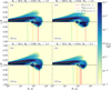 |
Fig. 1 CO gas and ice abundance distributions in the disk for four models with different model parameters. Contours represent τ = 1 surfaces of used lines. Upper left panel: reference model with Md = 0.01 M⊙, Rc = 50 au, and M⋆ = 1.0 M⊙. The other panels represent models with one parameter value different from the reference. Right upper panel: Rc = 100 au. Left lower panel: Md = 0.02 M⊙. Right lower panel: M⋆ = 1.5 M⊙. |
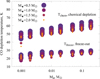 |
Fig. 2 Freeze-out and chemical depletion temperatures depending on the disk mass. |
3.2 Dependence of CO isotopologue emission on disk parameters
The variation of the model parameters has evident influence on the physical and chemical structure of the disk, in particular, on the abundance of CO isotopologues and, hence, on their line emission. In this section, the impact of each individual parameter on the physics and chemistry of the disk is further discussed in detail.
In Fig. 1, CO gas and ice abundance distributions and τ = 1 isolines for the considered molecular transitions are illustrated for four different models of our grid. One of the models is the “reference model” with average parameters in our grid (Md = 0.01 M⊙, Rc = 50 au, M⋆ = 1.0 M⊙) and the other three models explore the variation in the disk mass, size, and the mass of the central star. We calculated the optical depth in the lines of CO and its isotopologues, assuming the face-on disk observation. The τ = 1 isoline of CO and 13CO shift quite significantly due to the complex distribution of gas-phase CO in the molecular layer and the midplane, while the τ = 1 for C18O appears to be less sensitive to the variation of the disk model parameters.
Figure 3 shows the dependence of the line fluxes on the system parameters: disk mass, Md, characteristic disk radius, Rc, and star mass, M⋆ at a constant disk inclination of i = 60°. Solid lines refer to our grain-surface chemistry network. Dashed lines show the same dependences in the models without chemistry, where we followed WB14 and calculated the abundance of CO parametrically, assuming it is only restricted by freeze-out at 20 K and photodissociation. For the rest of the Section 3, we focus on the grain surface chemistry case only. We return to the comparison with the results of other authors in Section 4.
3.2.1 Disk inclination, i
Figure 4 demonstrates the dependence of the isotopologue line fluxes on the disk inclination for each set of fixed parameter values, as well as the maximum, minimum, and geometric mean of dependences at each inclination. For CO, on average, the flux is independent of the inclination up to i = 60°; whereas at larger angles, the flux drops slightly (by less than a factor of two). For C18O and 13CO, there is a slight rise (1.2F(i = 0°) at peak) of flux from 0° to 60° and then a similar drop. Due to the found weak dependence and the lack of qualitative influence on the dependences on the other parameters, we only considered the case of the most probable inclination: i = 60°.
The dependence can be explained the following way. On the one hand, increasing the inclination of the disk increases the amount of matter in the line of sight, while decreasing the total visible area of the disk. In the case of CO, it leads to a hotter, but smaller τ = 1 disk surface, along with the appearance of colder disk outer edge. In the case of C18O and 13CO, while we also see less of the disk surface, τ = 1 surface at low i can increase in size due to more matter in the line of sight in previously transparent areas; thus, the flux can slightly increase as well. For higher inclinations, the disk stops being transparent anywhere and the flux decreases, as in the case of CO.
On the other hand, the Doppler effect becomes more prominent as the projection of the rotational velocity component of the disk onto the line of sight increases. This redistributes the energy across the spectrum and reduces the optical depth at the central line frequencies, allowing us to see more matter overall. As a result, the flux increases. The combination of these two effects keeps the resulting flux constant at i < 60° for CO and slightly rising for C18O and 13CO. At i > 60°, the first effect becomes more significant and the flux drops.
3.2.2 Characteristic disk radius, Rc
Increasing the disk radius at a fixed disk mass (cf. upper panels of Fig. 1) leads to a redistribution of mass from the inner to the outer parts of the disk. The outer parts are colder and, at some distance from the star, CO gets depleted from the gas phase due to chemical depletion and freeze-out. Beyond a certain distance, where the temperature is lower than the Tchem value shown in Fig. 2, gas-phase CO abundance becomes low and it does not show any emission. As a result, larger disks, on the one hand, can have more flux due to more matter emitting from a larger disk surface; however, on the other hand, it can decrease due to the depletion of more CO.
The question of which of these factors will dominate depends on the optical depth of the line emission. If the line emission is optically thick, then a lot of matter is below the τ = 1 level and does not contribute to the total flux. Increasing the size of the disk brings some of this previously invisible matter into new regions and it becomes visible, which increases the flux. However, this redistribution shifts the τ = 1 surface closer to the midplane, where temperatures are lower, so the flux from the inner parts decreases slightly. This is the case of CO flux, which always increases with radius in the upper panels of Fig. 3. The emission in this line is so optically thick that the τ = 1 surface is almost coincident with the upper boundary of the molecular layer. Freezing has no effect on the flux in this line, since it occurs near the disk midplane, under the τ = 1 surface.
If the line emission is optically thin, then the redistribution of matter reduces the flux, since initially, the emission from almost all the matter is already observable, and with the disk size increased, the matter is redistributed to colder regions. The freeze-out also contributes to the flux decrease. This case is relevant to C18O in low-mass disks. In the lower panels of Fig. 3, its flux can be seen first falling with radius for low-mass disks and increasing after some disk mass value that depends on the stellar mass. The disk (particularly the inner disk) is not completely transparent in this line, but enlarging the disk lowers the optical depth enough to cause a noticeable loss of flux. At higher disk masses, however, the removal of matter from optically thick regions becomes more significant in its contribution to the flux. The case of 13CO is intermediate between CO and C18O.
Overall, in the optically thick case, the radius increase leads to an increase of the line flux. In the optically thin case, it causes a decrease in the line flux.
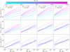 |
Fig. 3 Dependence of CO, 13CO, and C18O line fluxes on disk mass, disk radius, and stellar mass at the disk inclination, i = 60°. Solid lines show the results with a grain-surface chemistry network, while dashed lines are results with assumptions from WB14. |
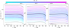 |
Fig. 4 Dependence of CO, 13CO, and C18O line fluxes on disk inclination. Along the individual colored lines, all parameters except the inclination are fixed. The black dashed lines show the maximum and minimum flux values at each inclination. Black solid lines show geometric mean of flux dependences. |
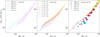 |
Fig. 5 Dependences of the CO line fluxes on the R90 at disk inclination i = 0° and stellar mass M⋆ = 1 M⊙. The left panel presents the dependences of fixed Rc, middle presents those of the fixed Md, and the right shows models of all Rc and Md differentiated by shade and size. |
3.2.3 Disk mass, Md
An increase in the disk mass (left panels of Fig. 1) leads to an increase in the absolute CO mass density in the entirety of the disk. This shifts the τ = 1 surface away from the star both radially and vertically, with the magnitude of this shift increasing with the radius of the disk, Rc. Temperature in the disk rises with height so flux increases from the entire τ = 1 surface which now is also larger. As a result, flux increases with disk mass in both optically thick and thin cases. This is also reflected in Fig. 3, where all line fluxes rise with disk mass. The temperature range of the CO-free region in the midplane increases with mass (see Fig. 2), but, the inner edge of this region, where CO becomes more depleted, is hidden under the τ = 1 surface and does not contribute much to the emission.
The influence of disk mass on its size can be seen through another observational characteristic, R90, which is defined as the radius of disk area that produces 90% of the CO flux. In Fig. 5, we show how R90 relates to the total CO flux FCO for models of all chosen Md and Rc at i = 0° and M⋆ = 1 M⊙. In the left panel, we can see how both R90 and FCO increase with disk mass at fixed Rc. Compared to the middle panel, which shows the same but with Rc changing and Md fixed, we see that the slope of FCO-R90 relation is different depending on which parameter is fixed. This points at other factors that influence flux besides sheer size and this factor is the increase in temperature at the τ = 1 surface (as stated above). The increase in Rc does not reflect a pure dependence of flux on size either, as it leads to a decrease in temperature at the τ = 1 surface (see Section 3.2.2). Hence, looking at a full picture on the right panel, we can conclude that the size of the disk cannot be accurately inferred from the CO flux alone, as it requires a knowledge of thermal structure that is influenced by both Md and Rc.
3.2.4 Stellar mass, M⋆
An increase in the mass of the star (left upper and right lower panels of Fig. 1) leads to a stronger gravitational field and an increase in luminosity. The enhanced gravitational field compresses the disk in the vertical direction and increases the rotation velocity of the disk. The compression of the disk shifts the τ = 1 surface closer to the midplane. A higher rotational velocity gives a higher Doppler shift of the lines, which distributes the energy more broadly across the spectrum, allowing more matter to be seen and, hence, the total flux increases. However, this only has an effect on a model with an inclination other than zero. The effect is greater for inclinations closer to 90°.
The increase in luminosity warms the disk to a higher temperature and increases the radiation field. It affects both CO emitting properties and local chemical reaction rates. With regard to the emission, higher temperature increases the source function value Sν, but decreases the number density of CO emitting in the line, since the maximum J = 2 level population of CO isotopologues corresponds to a temperature of ~17 K. This temperature is below a typical CO freeze-out temperature of 20 K; thus, it is impossible to find CO at such temperatures, except at the very periphery of the disk (>1000 au) where photodesorption is active. These are counteracting factors, since the intensity is Iν ∝ Sν (1 − e−τν). The factor that is, in fact, the dominant one depends on the disk radius, since the larger the disk is at a fixed disk mass, the more transparent it is.
Higher stellar luminosity means that CO depletion and freeze-out fronts move away from the star. The temperature of CO chemical depletion, Tchem, is lower in models with higher M⋆ (see Fig. 2), which means that the region of CO depletion between Tchem and Tfreeze shifts even further out. On the one hand, the increased area of the region inside Tchem contributes to the flux increase. On the other hand, it is counteracted by CO destruction that becomes more efficient as the disk’s scale height decreases with stellar mass. As the disk shrinks to the midplane due to stellar gravity, the molecular layer moves closer to the midplane and becomes thinner (see lower panels of Fig. 1), it is more affected by the chemical depletion, effective at the midplane temperatures and densities. CO abundance in the molecular layer decreases due to the combined effect of chemical depletion and photodissociation, which is more significant in large low-mass disks, where the molecular layer above the depleted region basically disappears. This effect decreases the CO flux, particularly in low-mass disks more transparent to dissociative UV radiation. At the same time, the intrinsic UV radiation field does not change much with the stellar mass, as it is dominated by the emission from the hotter accretion region with the temperature of 10 000 K.
Overall, stellar mass produces a range of effects with some working against each other in terms of flux. Which factors will overweigh the others depends on disk mass and radius, as well as the optical depth of the line in the CO depletion region. We discuss the effects of different contributions of stellar masses in more detail in Appendix B.
3.3 Approximation of emission dependence on disk mass
All the dependences in Fig. 3 can be approximately described by a linear regression in logarithmic scale of the following form,
![Mathematical equation: $\[\lg f_l=a_l+b_l \lg m_{\mathrm{d}},\]$](/articles/aa/full_html/2025/07/aa53529-24/aa53529-24-eq7.png) (3)
(3)
where ![Mathematical equation: $\[f_{l}=\frac{F_{l}}{1 ~\mathrm{mJy} ~\mathrm{km} / \mathrm{s}}, ~l\]$](/articles/aa/full_html/2025/07/aa53529-24/aa53529-24-eq8.png) is the line of any of the CO isotopologues, and
is the line of any of the CO isotopologues, and ![Mathematical equation: $\[m_{\mathrm{d}}=\frac{M_{\mathrm{d}}}{10^{-3} ~M_{\odot}}\]$](/articles/aa/full_html/2025/07/aa53529-24/aa53529-24-eq9.png) . In this case, the approximation coefficients al(Rc, M⋆) and bl(Rc, M⋆) will be functions of the remaining model parameters. This allows us to analyze the dependences in more detail and compare them with each other both for different lines and at different fixed values of the remaining parameters. The approximation is performed using the routine scipy.stats.linregress2.
. In this case, the approximation coefficients al(Rc, M⋆) and bl(Rc, M⋆) will be functions of the remaining model parameters. This allows us to analyze the dependences in more detail and compare them with each other both for different lines and at different fixed values of the remaining parameters. The approximation is performed using the routine scipy.stats.linregress2.
Figure 6 shows the result of the approximation of the data from Fig. 3, while Fig. 7 shows the dependence of the obtained coefficients, al and bl, on the radius Rc and mass of the star, M⋆. The intercept al is the flux for models with Md = 10−3 M⊙ by definition. For CO, al rises with stellar mass for smallest disks, which are least affected by increasing destruction in the molecular layer and benefit more from the increased temperature. As the disk size increases, chemical depletion and photodissociation in the molecular layer play a bigger role so the flux decreases with stellar mass for the largest disks. For C18O and 13CO, while the same factors come into play, the major contribution to flux comes from CO depletion area, which is fully transparent in both lines. Therefore, when stellar mass is increased, more CO is introduced to the disk and the disk is overall hotter, leading to significantly higher molecular flux. Dependence on the disk radius is in full accordance with explanations in Section 3.2.2.
The slope bl reflects the sensitivity of the flux to the disk mass and, hence, the possibility to determine the disk mass from the flux. Figure 7 shows that all lines are approximately equally sensitive to the disk mass. Additionally, the dependence on Rc does not change much with the stellar mass for CO line. The only exception for CO is presented by the largest disks which are most affected by molecular layer destruction. This effect decreases with disk mass and this leads to a change in slope. For C18O and 13CO, there is a minor decrease in slope with increasing stellar mass as massive disks are slightly less affected by factors described in the previous paragraph. For instance, it is harder to heat a more massive disk, hence, a smaller fraction of CO is desorbed. Finally, bl increases by a factor of 2–3 from the minimum radius to the maximum radius.
As a result, the fluxes in CO isotopologue lines can differ by an order of magnitude or more between models. Although the flux dependences on individual parameters are clearly distinguished, the coefficients depend on other parameters with a remaining scatter of one order of magnitude in the flux. Hence, it is not possible to accurately determine the value of any parameter from the flux in a single CO line without the knowledge of the other parameters. It is possible that the simultaneous use of several lines could allow for the determination of some parameters.
It is important to note here a seeming discrepancy between the conclusion of an earlier study by Molyarova et al. (2017) and our results. Molyarova et al. (2017) found that CO gas mass correlates well with total disk mass with correlation being stable against other parameters. As we used the same chemical model, the CO gas mass in our work behaves the same way. However, the flux also depends on the structure and temperature profile of the emitting surface. They are much more sensitive to model parameters, thereby giving way to the flux variations.
3.4 Using combinations of lines to determine disk parameters
The use of two CO lines to determine parameters, in particular disk masses, was previously proposed in WB14. The authors considered a set of disk models with different parameter values and modeled CO isotopologue line emission from them. They plotted the resulting line luminosities (Ll = 4πd2Fl, where d is the distance to the object) for C18O and 13CO on a luminosity diagram grouping them by disk mass (Fig. 6 of their work or Fig. 9 of this work). Here, we adopt a similar approach and Fig. 8 shows the results of our work on a such diagram. Besides the disk mass (upper left panel), we also group models by characteristic radius (upper middle) and stellar mass (upper right). Additionally, we provide parameter uncertainty distributions for the diagrams (lower panels). Parameter uncertainty for a chosen point on a diagram is defined as a ratio between the maximal and minimal parameter values of models within 10% range of luminosities of the chosen point (10% chosen as it is a typical absolute flux calibration error for ALMA). Given the ranges of values on our grid, the maximum possible uncertainties are 200, 16, and 4 for disk mass, characteristic radius and stellar mass, respectively.
Looking first at disk mass (left panels of Fig. 8), we see that while the increase in disk mass leads to an increase in luminosities of both lines, it is significantly smaller than the luminosity variation for a fixed mass (factor of two versus an order of magnitude). The result is an overlap of models of different mass up to models of lowest and highest mass meeting each other. This can be seen in the uncertainty distribution as well, where in the middle of the distribution there exists a spot with uncertainty of at least two orders of magnitude. While the spot does not seem large, it is important to note that its size is also determined by parameter ranges we use. Considering disks with a wider range of mass and size will inevitably expand this spot.
Moving to disk characteristic radius (middle panels of Fig. 8), models seem to group by this parameter much more distinctively compared to disk mass. This is because the 13CO line luminosity increases with radius for most of the models while for C18O line, the behavior is more mixed. The area occupied by the models is still rather localized; thus, in the uncertainty distribution, we can see a thin strip of maximum possible uncertainty of 16 in the middle. Substituting 13CO with CO, the luminosity of which increases with radius in all models, gives a better separation of models of different radii with maximum and average uncertainties, of 4 and 2, respectively (see right panel of Fig. 10). The overlap increases, however, towards lower disk masses and the uncertainty can reach 8 in some isolated points. It is possible that with disk mass range expanded towards lower values, the uncertainty will increase there even more as CO gets increasingly optically thin.
Lastly, stellar mass (right panels of Fig. 8) cannot be meaningfully differentiated in a luminosity diagram. Most of the uncertainty distribution is occupied by a maximum possible value of 4.
Concluding this analysis and considering the parameter grid limitations, using a combination of C18O and 13CO line luminosities can allow us to determine the disk mass within a factor of 100–50, characteristic radius within a factor of 16–8 and stellar mass within a factor of 4. Using CO instead of 13CO improves the uncertainty of the characteristic radius estimate to a factor of 4–2. Adding the variability inherent to T Tauri-type stars and outbursting events such as EXor and FUor outbursts, the scatter and uncertainty would increase even more.
However, the estimates can be improved by using additional information and parameter constraints from other wavelengths (stellar mass from the optical, disk mass from the dust continuum) and spatially resolved observations (for radius). At the same time, inclination can be safely ignored (Section 3.2.1). Results of our modeling (including R90) are compiled in Appendix A for the use by the community. Another option is to fit multiple observations with full physico-chemical models, such as in Thi et al. (2010) and Zhang et al. (2019).
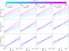 |
Fig. 6 Dependences of the CO, 13CO, and C18O line fluxes on the disk mass, disk radius, and stellar mass at disk inclination i = 60°. The dots represent model values of the fluxes and the lines show the approximation. |
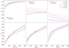 |
Fig. 7 Dependences of the approximation coefficients on the disk radius and stellar mass at disk inclination i = 60° for the CO, 13CO, and C18O lines. The vertical bars denote the uncertainty of the approximation coefficient. |
4 Discussion
In this section, we compare our results to previous works and observations and analyze how differences between model assumptions cause different outcomes.
4.1 Effect of model assumptions
The left panel of Fig. 9 shows a luminosity diagram with translucent points presenting results of WB14, traced points presenting our results with WB14 assumptions, traced star points presenting results of M16, and the contours marking the results of this work with the grain-surface chemistry network. Compared to WB14 and M16, the luminosities of our grain-surface chemistry models correspond to higher gas disk masses, with the shift being about one order of magnitude. This alleviates the current problem with CO mass estimation, which is that the masses from CO isotopologues are lower by 1–2 orders of magnitude than those derived from other molecular tracers (e.g., HD) (Trapman et al. 2022). There is also a higher degree of overlap between our models of different mass which we explore separately in Section 3.4.
At the same time, our results with the assumptions of WB14 align with their results quite well. In Fig. 3, we also show how flux under WB14 assumptions depends on disk parameters in comparison to the results of our grain-surface chemistry network. Comparing the two approaches, emission in the main CO isotopologue line is the least affected. While the dependence on radius for low-mass disks is noticeably different, the difference in flux between two models with the same parameters is within a factor of two. Emission in the 13CO and C18O lines is affected more significantly and the differences in flux between models with and without chemistry reach a factor of 3 and 5, respectively. Moreover, for all disk masses, the flux dependences on disk radius and stellar mass are completely different.
The line fluxes predicted by our models are different from those obtained in previous studies, as we use different model assumptions. The main differences are as follows. First, unlike WB14, both we and M16 use chemical network to calculate the CO abundances, which accounts for processes beyond thermal desorption, freeze-out and photo-dissociation. Second, our grain chemistry includes more complex processes than hydrogenation included by M16, particularly the CO chemical depletion, through surface conversion to CO2 (Bosman et al. 2018). Third, the disk vertical structure in our model (and in WB14) is determined by hydrostatic equilibrium and calculated self-consistently with temperature, instead of being parametrically set. Finally, our model lacks the inclusion of the isotope-selective processes of M16. Below we will disentangle the effects of these assumptions on the line fluxes, using different intermediate models that share some of the assumptions.
We use a baseline model with the same system parameters: Md = 0.01 M⊙, Rc = 60 au, M⋆ = 1.0 M⊙, L⋆ = 1.0 L⊙, and T⋆ = 4000 K. One deviation from this model is the vertical structure: we use the same Gaussian parametrization as M16 and refer to such models as “no HE” (no hydrostatic equilibrium) models. Another model variation is the models with reactions on dust grain surface turned off. We also explore the WB14 approach with no chemistry. Finally, we test the effect of isotopologue selective photodissociation by adopting different depletion levels of 13CO and C18O based of shielding factors by Visser et al. (2009). This allows us to assess the effect of isotopologue-selective processes in the disk upper layers at postprocessing.
The line luminosities of these test models are presented in the left panel of Fig. 9. The model marked by a black point is our grain-surface chemistry model. There are two main variations of this model, marked by red and black arrows: one with parametric vertical structure (hc = 0.1, ψ = 0.1) and one with grain-surface reactions off. Both parametric structure and no grain-surface reactions give an increase in flux for both lines, with surface chemistry having a stronger effect (a factor of 2–3 increase versus a factor of 1.5). Combining both modifications further increases the flux. These effects are illustrated in more detail in Appendix C. Finally, there is a model with assumptions from WB14 that has the highest flux among all test models, as it accounts for minimum CO depletion level.
Additionally, each model except for the one with WB14 assumptions was tested for the effect of isotopologue-selective photodissociation (marked by blue arrows). We assume that the abundances of CO isotopologues in the upper disk layers are determined by photodissociation (M16) and the relative species abundances are inversely proportional to the photodissociation rates. In these models, we artificially reduce the fraction of the isotopologue by a factor of θCO/θ13CO and θCO/θC18O, in the layer with θ13CO or θC18O above 10−2. Here, θX is the shielding factor for the molecule X, calculated from the parameterization provided by Visser et al. (2009), see their Table 5. The values of the applied reduction factor vary across the disk, ranging from ≈ 1 in the upper layers, where shielding is not yet efficient to ≈ 10 deeper in the molecular layer. In all cases inclusion of this approximation leads to a decrease in the rare isotopologue abundances in the upper layers (by a typical factor of ~2–3), and consequently to the decrease in their fluxes. The difference is around a factor 1.2–1.5 for both isotopologues, which is much lower than the effect of chemical processes. However, selective photodissociation is not the only effect of isotopologue chemistry. Other isotopologue selective chemical reactions can also increase the abundances, for instance, by a factor of ~2 for 13CO, as was shown by Miotello et al. (2014). However, they are hard to assess without running full isotopologue-selective chemical network, so we limited our analysis to the effect of photodissociation. The fluxes in the M16 models are also higher than in our simulations (see Fig. 10) due to their use of parametric vertical structure, which increases the fluxes (red arrows in Fig. 9).
Observed fluxes of CO isotopologues can be affected by other physical processes unaccounted for in our modeling. One of the most important factors is the thermal structure of the disk, which can be different from the adopted parametrization. First, the disk thermal structure can have a significant effect on CO freeze-out and the level of CO depletion. For example, the existence of a thick vertically isothermal layer around the disk midplane has been suggested based on the observational data and would also affect the emission of CO and its isotopologues (Qi et al. 2019; Qi & Wilner 2024). Vertical mixing, radial drift, and dust settling can also enhance CO depletion (Zhang et al. 2019; Krijt et al. 2020), even without processing to CO2 (Van Clepper et al. 2022). Different adsorption rates to dust grains of different sizes can also increase the CO depletion from the gas phase (Powell et al. 2022). Similarly, adsorption favors larger grains due to their lower temperatures (Kalvāns 2025), which could also contribute to the level of depletion.
Substructures, such as rings or spirals can form in the disk even before 1 Myr age, affecting its physical structure and consequently the chemical depletion rates. At longer timescales, other processes can become important, such as disk photoevaporation, stellar evolution, disk-planet interaction, and (most notably) dust evolution. Gas-phase CO can also be significantly depleted by magnetic winds (Jonczyk et al., in prep.). Each of these effects can affect the abundances of CO and the isotopologues and the timescales of chemical reactions. We considered a 1 Myr old Class II disk, where these effects can be overlooked to some degree. Nevertheless, the inclusion of the above processes can significantly affect CO abundances and the level of depletion in a particular disk, increasing the degree of uncertainty in the disk parameter determination.
In conclusion, the difference in the derived luminosities compared to WB14 and M16 can be explained by the combination of chemistry, particularly on the dust surface, vertical disk structure, and isotopologue-selective processes. We show that the most significant contribution comes from surface chemistry, in particular, the mechanism of CO conversion to CO2 on dust.
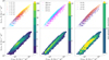 |
Fig. 8 Luminosity diagrams for the C18O and 13CO lines in our models. Upper left: model fluxes are grouped by disk mass and contours outline the regions where models of corresponding mass reside. Upper middle: models are colored according to characteristic radius. Upper right: Models are colored according to stellar mass. Lower left: distribution of uncertainty in disk mass. Lower middle: uncertainty in characteristic radius. Lower right: uncertainty in stellar mass. Uncertainty here is defined as the ratio of maximum and minimum parameter value within 10% range of luminosities of the point on the diagram. White means there are no models nearby. |
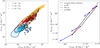 |
Fig. 9 Luminosity diagrams for the C18O and 13CO lines. Left: translucent points are results of WB14 assuming CO/C18O = 550 and traced points are results of this work using the assumptions from WB14. Traced stars are results of M16 and contours are results of this work with the grain-surface chemistry network. The points and contours are colored according to the disk mass of the model. Right: points are values of individual test models. Black point is the grain-surface chemistry model, white points are modified versions of it. Color of the arrow shows the added modification to the model: grain chemistry turned off (black), parametric vertical structure (no HE, red), isotope-selective photodissociation (ISO on, blue), and the assumptions of WB14 (as WB14, gray). All models have the same parameters: Md = 0.01 M⊙, Rc = 60 au, M⋆ = 1.0 M⊙, L⋆ = 1.0 L⊙, and T⋆ = 4000 K. Models with parametric vertical structure have hc = 0.1, ψ = 0.1. |
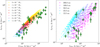 |
Fig. 10 Left: luminosity diagram for the C18O and 13CO lines. Translucent points are results of this work with grain-surface chemistry network The points are colored according to the disk mass of the model. Markers with errorbars are observations compiled in Zwicky et al. (2024) and from Ansdell et al. (2016). Right: luminosity diagram in the C18O and CO lines. All points are results of this work with grain-surface chemistry network and colored according to the Rc. Markers with errorbars are observations compiled in Zwicky et al. (2024). |
4.2 Measuring disk masses and radii
In Fig. 10, we plot some observations of T Tauri disks compiled in Zwicky et al. (2024) (Dutrey et al. 1997; Williams & Best 2014; Ansdell et al. 2017; Grant et al. 2021; Pegues et al. 2021; Semenov et al. 2024) and from Ansdell et al. (2016) as markers with errorbars. We see that the majority of objects overlap with our data points with a few having either higher 13CO luminosity or higher luminosity in both lines. Considering larger and more massive model disks can help reproduce the values observed in these objects. Such massive disks are not included in our modeling, as the assumptions made for the disk structure would not be appropriate for the self-gravitating disks. Besides, masses of the most massive disks can be determined more directly, from their kinematic structure (Veronesi et al. 2024). Finally, recent FUor outbursts can increase flux in both of these lines (Zwicky et al. 2024). Some of the objects in the plot, namely CI Tau, [MGM2012] 556 and IM Lup, are considered to be post-FUor candidates based on the elevated C18O/CO and 13CO/CO flux ratios so their parameters can be overestimated using this method.
In the right panel of Fig. 10, we present a similar luminosity diagram but with 13CO substituted by CO and only with our grain-surface chemistry results. Markers with errorbars are observations compiled in Zwicky et al. (2024). Here, we also see our model set covering most of the observational values, making it possible to give some estimates of the characteristic radius. In Appendix A, we present a table with these estimates for both R90 and Rc. It is important to note that per Zwicky et al. (2024) predictions, outbursts in the past could lead to a lower radius estimate when using this method.
Our results are directly related to the problem of measuring disk gas masses and radii, which are one of the key goals of the upcoming ALMA large programs AGE-PRO (Zhang et al. 2024) and DECO (Law et al. 2025). AGE-PRO and DECO observations are planned to be converted into masses using a method by Trapman et al. (2022). This method involves obtaining disk structure from SEDs and resolved observations, then constraining possible values of CO abundance and disk mass using C18O flux and finally determining both of them from N2H+/C18O flux ratio. Their model uses a chemical network similar to M16, which does not describe the chemical depletion of CO on the dust surface. Instead, they account for any unspecified source of CO depletion by setting global gas-phase CO abundance as a fitting parameter. However, this may not be sufficient as flux is sensitive to the thermal profile of the emitting area and (as we show above and in Appendix C) it depends on the presence of surface chemistry. We would like to emphasize here that careful consideration of CO depletion processes is crucial to accuracy of mass estimation methods and its inclusion to the models can be beneficial for the accuracy of the mass determination.
Another method and a whole tool for determining disk mass is the one proposed by Deng et al. (2023). Their model chemistry is based on the work by Ruaud et al. (2022), with a more extensive chemical network, including some isotopologue-specific reactions. It is difficult to compare our results due to different approaches to the disk parameter space exploration. Beyond the disk mass, Ruaud et al. (2022) vary only dust-to-gas mass ratio and outer disk radius. We, on the other hand, consider only one value of dust-to-gas ratio and vary characteristic radius instead of the disk outer rim. However, the dependences of isotopologue flux on disk mass is in agreement with ours and of similar amplitude. The simplified model they construct is checked to be roughly in line with their full chemical model, so our results are in approximate agreement with it as well. This may be attributed to the inclusion in the model of hydrostatic equilibrium and CO depletion through conversion to CO2, as we have in our models. Ruaud et al. (2022) concluded that C18O can be a good measure of disk gas mass given that there are good constraints on other model parameters from other sources, which is in agreement with the results of the present study.
5 Conclusions
In this work, we explored how the line fluxes of various CO isotopologues are affected by varying disk mass and radius, stellar mass, and inclination. Using the astrochemical model ANDES (Akimkin et al. 2013) and the radiative transfer code RADMC-3D (Dullemond et al. 2012), we simulated flux in CO, 13CO, and C18O J = 2–1 lines on a grid of models of varying disk mass, Md, and radius, Rc, inclination, i, and stellar mass, M⋆. We explored the dependences of flux on inclination and disk mass with other parameters fixed. We provided physical and chemical explanations for the influence of each varied parameter. We approximated the dependences on disk mass loglinearly and described how coefficients of approximations change with disk radius and stellar mass. We tested whether the combinations of lines can be used to estimate parameters similar to the methodology of Williams & Best (2014). Finally, we compared our results to Williams & Best (2014), Miotello et al. (2016), and the observations. We explored the main reasons behind differences in our results. Our findings can be summarized as follows:
The flux in all lines is independent of inclination for i < 60°. For i > 60°, it decreases with higher inclinations but within a factor of < 2;
The flux in all lines increases with disk mass;
The CO flux increases with disk radius, while 13CO and C18O flux dependence on it is more complex and it depends on both disk and stellar mass due to a combined effect of CO depletion area, temperature, and photodissociation on these more optically thin lines;
Due to these dependences, the use of just one line cannot provide reliable estimates of any parameter. However, having prior constraints on some parameters can improve the quality of the estimate;
Using 13CO-C18O line combination as per Williams & Best (2014) cannot produce reliable estimates of disk mass or radius as our grid of models disks of different mass and radius heavily overlap in luminosity. Using a CO-C18O line combination can give an estimate of disk characteristic radius within a factor of 2–4;
Chemical depletion of CO leads to CO absent in both gas and ice phases at temperatures below 34–65 K and above the freeze-out temperature of 17–29 K, with the certain values depending on the model parameters. It is caused by the transformation to CO2 on the dust grain surface;
The inclusion of surface chemistry significantly reduces 13CO and C18O isotopologue flux as their emission traces the region of chemical CO depletion. This reduction in flux is a major source of a systematic underestimation of disk mass in previous works. A choice in disk vertical structure description also impacts the flux. A structure from hydrostatic equilibrium gives a lower 13CO and C18O flux compared to parametric prescription.
Data availability
The model parameters, R90, and flux data shown in Table A.1 are available at https://doi.org/10.5281/zenodo.15690896. Additional data can be provided upon request to the corresponding authors.
Acknowledgements
We are thankful to the anonymous referee for their constructive comments and suggestions that helped to improve the manuscript. L. Zwicky, P. Ábrahám, and Á. Kóspál acknowledge financial support from the Hungarian NKFIH OTKA project no. K-147380. T. Molyarova was supported by the Royal Society, award numbers URFVR1/211799 and RF\textbackslash ERE\textbackslash 231082. The research leading to these results has received funding from the European Union’s Horizon 2020 research and innovation programme under Grant Agreement 101004719 (ORP). This work was also supported by the NKFIH NKKP grant ADVANCED 149943 and the NKFIH excellence grant TKP2021-NKTA-64. Project no. 149943 has been implemented with the support provided by the Ministry of Culture and Innovation of Hungary from the National Research, Development and Innovation Fund, financed under the NKKP ADVANCED funding scheme. This publication is based upon work from COST Action PLANETS CA22133, supported by COST (European Cooperation in Science and Technology).
Appendix A Model data and estimates
Table A.1 contains all the computed grain-surface chemistry models with their parameters, fluxes and R90. Table A.2 presents our estimates of R90 and Rc for a subset of observations compiled in Zwicky et al. (2024). Estimates are obtained by taking minimum and maximum parameter values of the models within errorbars of the objects. If there are no models within object errorbars, an estimate cannot be made and such objects are not listed in the table.
Parameters, R90 and fluxes of the grid of models.
Estimates of R90 and Rc for a set of observations compiled in Zwicky et al. (2024).
Appendix B Disentangling stellar mass effects
The effect of stellar mass consists of three contributions: disk thermal structure, vertical distribution of gas, and velocity field. To disentangle these three effects, we consider three sets of models. The first set includes twelve models with Md = 0.01 M⊙, Rc = 50 au, four values of M⋆ = 0.5, 1, 1.5, 2 M⊙ and three inclinations i = 0°, 45°, 90°. These models will experience all the three effects of different stellar mass. For the second set, we run the same twelve models, but with fixed T⋆ = 4000 K and L⋆ = 1 L⊙. This eliminates the effect on the thermal structure, but the vertical density distribution and velocity field in the models are still affected by the stellar mass. Finally, in the third set of models, we simulate the model with M⋆ = 1 M⊙, but assume the disk to have velocity distributions corresponding to the four different values of M⋆ (at three different inclinations). This set of models will only include the effect of the kinematic structure.
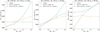 |
Fig. B.1 Dependence of the CO flux on the stellar mass for three inclinations. Left panel: i = 0°. Middle panel: i = 45°. Right panel: i = 90°. Three types of models are considered: original, with grain-surface chemistry, from Table A.1; models where temperature and luminosity of the star were fixed to T⋆ = 4000 K and L⋆ = 1 L⊙; models where only velocity field was adjusted to stellar mass. |
Effects of photodissociation are fully included in the “original” set of models, both due to the change in stellar temperature (minor) and combined destruction of CO in the molecular layer on dust grain surface and by photodissociation. Effects of photodissociation can also change in the second set of models, as the radiation field distribution will shift according to the density change as the disk scale height decreases, possibly destroying more CO in the upper disk layers.
Fig. B.1 shows the dependences of CO fluxes on stellar mass in these sets of models. First we consider the case of i = 0° (left panel). As the disk is face-on and we do not see disk rotation in the line profile, the flux is constant for the third set of models. When we add influence of mass on the vertical density structure, flux starts to increase with star mass (F(2 M⊙)/F(0.5 M⊙) = 1.15) due to a temperature increase along τ = 1 surface as the density structure affects the radiation field. Lastly, adding the thermal effect, flux increases more (F(2 M⊙)/F(0.5 M⊙) = 1.32) as the disk surface heats up.
For i = 45° (middle panel), we start to see the effect on flux from the Doppler shift (F(2 M⊙)/F(0.5 M⊙) = 1.2). Including disk compression now decreases the effect on flux (F(2 M⊙)/F(0.5 M⊙) = 1.15) as a part of the emission surface is the disk outer rim which shrinks with higher stellar mass. Adding the thermal effect raises the flux increase rate further (F(2 M⊙)/F(0.5 M⊙) = 1.32).
Finally, in i = 90° (right panel) case, Doppler shift has its highest effect (F(2 M⊙)/F(0.5 M⊙) = 1.5). Disk compression, however, completely negates it as now we see only the disk outer rim. In the end we are left with the flux increase from pure thermal effect (F(2 M⊙)/F(0.5 M⊙) = 1.13).
Concluding, all three effects give comparable flux change with disk compression acting against the flux increase from rest at higher inclinations and adding to it at lower.
Appendix C Parametric vertical structure and no grain-surface reactions
Fig. C.1 presents CO gas and ice distributions for four models from Fig. 9 right panel. The model in the left upper panel is our reference model with grain-surface chemistry and hydrostatic equilibrium. If we now set the vertical structure parametrically (left lower panel), we see that the τ = 1 surfaces shift upwards where temperature is slightly higher which contributes to the flux increase. For C18O we also see a slight shift of the τ = 1 surface from the star. This can be explained by more matter being above the depletion area as scale height is higher in this case.
When we turn off grain-surface reactions (right upper panel), the region of CO depletion between Tfreeze and Tchem (see Section 3.1) becomes rich in CO gas (from 10 to 50 au in the presented model). This evidently expands the emitting area for 13CO and C18O, thus increasing the flux. Combining both effects (right lower panel) further increases the fluxes.
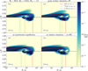 |
Fig. C.1 CO gas and ice abundance distributions in the disk for four models with different assumptions but same parameters. Contours represent τ = 1 surfaces of used lines. Left upper panel: a reference model with grain-surface chemistry and Md = 0.01 M⊙, Rc = 60 au, M⋆ = 1.0 M⊙. Right upper panel: no grain-surface reactions. Left lower panel: parametric vertical structure. Right lower panel: parametric vertical structure and no surface chemistry. |
References
- Akimkin, V., Zhukovska, S., Wiebe, D., et al. 2013, ApJ, 766, 8 [NASA ADS] [CrossRef] [Google Scholar]
- Andrews, S. M., & Williams, J. P. 2005, ApJ, 631, 1134 [Google Scholar]
- Ansdell, M., Williams, J. P., van der Marel, N., et al. 2016, ApJ, 828, 46 [Google Scholar]
- Ansdell, M., Williams, J. P., Manara, C. F., et al. 2017, AJ, 153, 240 [Google Scholar]
- Bergin, E. A., Cleeves, L. I., Gorti, U., et al. 2013, Nature, 493, 644 [Google Scholar]
- Bitsch, B., Lambrechts, M., & Johansen, A. 2015, A&A, 582, A112 [NASA ADS] [CrossRef] [EDP Sciences] [Google Scholar]
- Bohlin, R. C., Savage, B. D., & Drake, J. F. 1978, ApJ, 224, 132 [Google Scholar]
- Booth, A. S., Walsh, C., Terwisscha van Scheltinga, J., et al. 2021, Nat. Astron., 5, 684 [NASA ADS] [CrossRef] [Google Scholar]
- Bosman, A. D., Walsh, C., & van Dishoeck, E. F. 2018, A&A, 618, A182 [NASA ADS] [CrossRef] [EDP Sciences] [Google Scholar]
- Bruderer, S., Doty, S. D., & Benz, A. O. 2009, ApJS, 183, 179 [Google Scholar]
- Cuppen, H. M., Walsh, C., Lamberts, T., et al. 2017, Space Sci. Rev., 212, 1 [Google Scholar]
- Deng, D., Ruaud, M., Gorti, U., & Pascucci, I. 2023, ApJ, 954, 165 [NASA ADS] [CrossRef] [Google Scholar]
- Dullemond, C. P., Juhasz, A., Pohl, A., et al. 2012, RADMC-3D: A multipurpose radiative transfer tool, Astrophysics Source Code Library [record ascl:1202.015] [Google Scholar]
- Dutrey, A., Guilloteau, S., & Guelin, M. 1997, A&A, 317, L55 [NASA ADS] [Google Scholar]
- Eistrup, C., Walsh, C., & van Dishoeck, E. F. 2016, A&A, 595, A83 [NASA ADS] [CrossRef] [EDP Sciences] [Google Scholar]
- Evans, L., Booth, A. S., Walsh, C., et al. 2025, ApJ, 982, 62 [Google Scholar]
- Favre, C., Cleeves, L. I., Bergin, E. A., Qi, C., & Blake, G. A. 2013, ApJ, 776, L38 [Google Scholar]
- Grant, S. L., Espaillat, C. C., Wendeborn, J., et al. 2021, ApJ, 913, 123 [NASA ADS] [CrossRef] [Google Scholar]
- Harsono, D., Bruderer, S., & van Dishoeck, E. F. 2015, A&A, 582, A41 [NASA ADS] [CrossRef] [EDP Sciences] [Google Scholar]
- Kalvāns, J. 2025, A&A, 694, A213 [NASA ADS] [CrossRef] [EDP Sciences] [Google Scholar]
- Kama, M., Trapman, L., Fedele, D., et al. 2020, A&A, 634, A88 [NASA ADS] [CrossRef] [EDP Sciences] [Google Scholar]
- Krijt, S., Bosman, A. D., Zhang, K., et al. 2020, ApJ, 899, 134 [NASA ADS] [CrossRef] [Google Scholar]
- Law, C., Cleeves, L. I., & DECO Team. 2025, in American Astronomical Society Meeting Abstracts, 245, 206.04 [Google Scholar]
- Leemker, M., van’t Hoff, M. L. R., Trapman, L., et al. 2021, A&A, 646, A3 [EDP Sciences] [Google Scholar]
- Mathis, J. S., Rumpl, W., & Nordsieck, K. H. 1977, ApJ, 217, 425 [Google Scholar]
- McClure, M. K., Bergin, E. A., Cleeves, L. I., et al. 2016, ApJ, 831, 167 [Google Scholar]
- Miotello, A., Bruderer, S., & van Dishoeck, E. F. 2014, A&A, 572, A96 [NASA ADS] [CrossRef] [EDP Sciences] [Google Scholar]
- Miotello, A., van Dishoeck, E. F., Kama, M., & Bruderer, S. 2016, A&A, 594, A85 [NASA ADS] [CrossRef] [EDP Sciences] [Google Scholar]
- Miotello, A., Kamp, I., Birnstiel, T., Cleeves, L. C., & Kataoka, A. 2023, in Protostars and Planets VII, eds. S. Inutsuka, Y. Aikawa, T. Muto, K. Tomida, & M. Tamura, Astronomical Society of the Pacific Conference Series, 534, 501 [NASA ADS] [Google Scholar]
- Molyarova, T., Akimkin, V., Semenov, D., et al. 2017, ApJ, 849, 130 [Google Scholar]
- Molyarova, T., Akimkin, V., Semenov, D., et al. 2018, ApJ, 866, 46 [NASA ADS] [CrossRef] [Google Scholar]
- Mordasini, C., Alibert, Y., Benz, W., Klahr, H., & Henning, T. 2012, A&A, 541, A97 [NASA ADS] [CrossRef] [EDP Sciences] [Google Scholar]
- Nomura, H., Tsukagoshi, T., Kawabe, R., et al. 2016, ApJ, 819, L7 [Google Scholar]
- Öberg, K. I., Guzmán, V. V., Walsh, C., et al. 2021, ApJS, 257, 1 [CrossRef] [Google Scholar]
- Öberg, K. I., Facchini, S., & Anderson, D. E. 2023, ARA&A, 61, 287 [CrossRef] [Google Scholar]
- Padovani, M., Ivlev, A. V., Galli, D., & Caselli, P. 2018, A&A, 614, A111 [NASA ADS] [CrossRef] [EDP Sciences] [Google Scholar]
- Pegues, J., Öberg, K. I., Bergner, J. B., et al. 2021, ApJ, 911, 150 [NASA ADS] [CrossRef] [Google Scholar]
- Powell, D., Gao, P., Murray-Clay, R., & Zhang, X. 2022, Nat. Astron., 6, 1147 [CrossRef] [Google Scholar]
- Qi, C., & Wilner, D. J. 2024, ApJ, 977, 60 [Google Scholar]
- Qi, C., Öberg, K. I., Espaillat, C. C., et al. 2019, ApJ, 882, 160 [Google Scholar]
- Ruaud, M., Gorti, U., & Hollenbach, D. J. 2022, ApJ, 925, 49 [NASA ADS] [CrossRef] [Google Scholar]
- Schöier, F. L., van der Tak, F. F. S., van Dishoeck, E. F., & Black, J. H. 2005, A&A, 432, 369 [Google Scholar]
- Semenov, D., & Wiebe, D. 2011, ApJS, 196, 25 [Google Scholar]
- Semenov, D., Henning, T., Guilloteau, S., et al. 2024, A&A, 685, A126 [NASA ADS] [CrossRef] [EDP Sciences] [Google Scholar]
- Tazzari, M., Testi, L., Natta, A., et al. 2017, A&A, 606, A88 [NASA ADS] [CrossRef] [EDP Sciences] [Google Scholar]
- Testi, L., Birnstiel, T., Ricci, L., et al. 2014, in Protostars and Planets VI, eds. H. Beuther, R. S. Klessen, C. P. Dullemond, & T. Henning, 339 [Google Scholar]
- Thi, W. F., Mathews, G., Ménard, F., et al. 2010, A&A, 518, L125 [NASA ADS] [CrossRef] [EDP Sciences] [Google Scholar]
- Trapman, L., Miotello, A., Kama, M., van Dishoeck, E. F., & Bruderer, S. 2017, A&A, 605, A69 [NASA ADS] [CrossRef] [EDP Sciences] [Google Scholar]
- Trapman, L., Zhang, K., van’t Hoff, M. L. R., Hogerheijde, M. R., & Bergin, E. A. 2022, ApJ, 926, L2 [NASA ADS] [CrossRef] [Google Scholar]
- Van Clepper, E., Bergner, J. B., Bosman, A. D., Bergin, E., & Ciesla, F. J. 2022, ApJ, 927, 206 [NASA ADS] [CrossRef] [Google Scholar]
- Veronesi, B., Longarini, C., Lodato, G., et al. 2024, A&A, 688, A136 [NASA ADS] [CrossRef] [EDP Sciences] [Google Scholar]
- Visser, R., van Dishoeck, E. F., & Black, J. H. 2009, A&A, 503, 323 [NASA ADS] [CrossRef] [EDP Sciences] [Google Scholar]
- Wakelam, V., Loison, J. C., Herbst, E., et al. 2015, ApJS, 217, 20 [NASA ADS] [CrossRef] [Google Scholar]
- Weidenschilling, S. J. 1977, Ap&SS, 51, 153 [Google Scholar]
- Williams, J. P., & Best, W. M. J. 2014, ApJ, 788, 59 [Google Scholar]
- Williams, J. P., & Cieza, L. A. 2011, ARA&A, 49, 67 [Google Scholar]
- Yorke, H. W., & Bodenheimer, P. 2008, in Massive Star Formation: Observations Confront Theory, eds. H. Beuther, H. Linz, & T. Henning, Astronomical Society of the Pacific Conference Series, 387, 189 [Google Scholar]
- Zhang, K., Bergin, E. A., Schwarz, K., Krijt, S., & Ciesla, F. 2019, ApJ, 883, 98 [Google Scholar]
- Zhang, K., Trapman, L., Pascucci, I., et al. 2024, in American Astronomical Society Meeting Abstracts, 244, 109.07 [Google Scholar]
- Zwicky, L., Molyarova, T., Akimkin, V., et al. 2024, MNRAS, 527, 7652 [Google Scholar]
All Tables
Estimates of R90 and Rc for a set of observations compiled in Zwicky et al. (2024).
All Figures
|
Fig. 1 CO gas and ice abundance distributions in the disk for four models with different model parameters. Contours represent τ = 1 surfaces of used lines. Upper left panel: reference model with Md = 0.01 M⊙, Rc = 50 au, and M⋆ = 1.0 M⊙. The other panels represent models with one parameter value different from the reference. Right upper panel: Rc = 100 au. Left lower panel: Md = 0.02 M⊙. Right lower panel: M⋆ = 1.5 M⊙. |
| In the text | |
|
Fig. 2 Freeze-out and chemical depletion temperatures depending on the disk mass. |
| In the text | |
|
Fig. 3 Dependence of CO, 13CO, and C18O line fluxes on disk mass, disk radius, and stellar mass at the disk inclination, i = 60°. Solid lines show the results with a grain-surface chemistry network, while dashed lines are results with assumptions from WB14. |
| In the text | |
|
Fig. 4 Dependence of CO, 13CO, and C18O line fluxes on disk inclination. Along the individual colored lines, all parameters except the inclination are fixed. The black dashed lines show the maximum and minimum flux values at each inclination. Black solid lines show geometric mean of flux dependences. |
| In the text | |
|
Fig. 5 Dependences of the CO line fluxes on the R90 at disk inclination i = 0° and stellar mass M⋆ = 1 M⊙. The left panel presents the dependences of fixed Rc, middle presents those of the fixed Md, and the right shows models of all Rc and Md differentiated by shade and size. |
| In the text | |
|
Fig. 6 Dependences of the CO, 13CO, and C18O line fluxes on the disk mass, disk radius, and stellar mass at disk inclination i = 60°. The dots represent model values of the fluxes and the lines show the approximation. |
| In the text | |
|
Fig. 7 Dependences of the approximation coefficients on the disk radius and stellar mass at disk inclination i = 60° for the CO, 13CO, and C18O lines. The vertical bars denote the uncertainty of the approximation coefficient. |
| In the text | |
|
Fig. 8 Luminosity diagrams for the C18O and 13CO lines in our models. Upper left: model fluxes are grouped by disk mass and contours outline the regions where models of corresponding mass reside. Upper middle: models are colored according to characteristic radius. Upper right: Models are colored according to stellar mass. Lower left: distribution of uncertainty in disk mass. Lower middle: uncertainty in characteristic radius. Lower right: uncertainty in stellar mass. Uncertainty here is defined as the ratio of maximum and minimum parameter value within 10% range of luminosities of the point on the diagram. White means there are no models nearby. |
| In the text | |
|
Fig. 9 Luminosity diagrams for the C18O and 13CO lines. Left: translucent points are results of WB14 assuming CO/C18O = 550 and traced points are results of this work using the assumptions from WB14. Traced stars are results of M16 and contours are results of this work with the grain-surface chemistry network. The points and contours are colored according to the disk mass of the model. Right: points are values of individual test models. Black point is the grain-surface chemistry model, white points are modified versions of it. Color of the arrow shows the added modification to the model: grain chemistry turned off (black), parametric vertical structure (no HE, red), isotope-selective photodissociation (ISO on, blue), and the assumptions of WB14 (as WB14, gray). All models have the same parameters: Md = 0.01 M⊙, Rc = 60 au, M⋆ = 1.0 M⊙, L⋆ = 1.0 L⊙, and T⋆ = 4000 K. Models with parametric vertical structure have hc = 0.1, ψ = 0.1. |
| In the text | |
|
Fig. 10 Left: luminosity diagram for the C18O and 13CO lines. Translucent points are results of this work with grain-surface chemistry network The points are colored according to the disk mass of the model. Markers with errorbars are observations compiled in Zwicky et al. (2024) and from Ansdell et al. (2016). Right: luminosity diagram in the C18O and CO lines. All points are results of this work with grain-surface chemistry network and colored according to the Rc. Markers with errorbars are observations compiled in Zwicky et al. (2024). |
| In the text | |
|
Fig. B.1 Dependence of the CO flux on the stellar mass for three inclinations. Left panel: i = 0°. Middle panel: i = 45°. Right panel: i = 90°. Three types of models are considered: original, with grain-surface chemistry, from Table A.1; models where temperature and luminosity of the star were fixed to T⋆ = 4000 K and L⋆ = 1 L⊙; models where only velocity field was adjusted to stellar mass. |
| In the text | |
|
Fig. C.1 CO gas and ice abundance distributions in the disk for four models with different assumptions but same parameters. Contours represent τ = 1 surfaces of used lines. Left upper panel: a reference model with grain-surface chemistry and Md = 0.01 M⊙, Rc = 60 au, M⋆ = 1.0 M⊙. Right upper panel: no grain-surface reactions. Left lower panel: parametric vertical structure. Right lower panel: parametric vertical structure and no surface chemistry. |
| In the text | |
Current usage metrics show cumulative count of Article Views (full-text article views including HTML views, PDF and ePub downloads, according to the available data) and Abstracts Views on Vision4Press platform.
Data correspond to usage on the plateform after 2015. The current usage metrics is available 48-96 hours after online publication and is updated daily on week days.
Initial download of the metrics may take a while.