| Issue |
A&A
Volume 698, June 2025
|
|
|---|---|---|
| Article Number | A71 | |
| Number of page(s) | 10 | |
| Section | Stellar structure and evolution | |
| DOI | https://doi.org/10.1051/0004-6361/202453378 | |
| Published online | 28 May 2025 | |
Discovery of a bimodal luminosity distribution in the persistent Be/X-ray pulsar 2RXP J130159.6–635806
1
Department of Physics and Astronomy, FI-20014 University of Turku, Finland
2
School of Physical Sciences and Centre for Astrophysics & Relativity, Dublin City University, Glasnevin D09 W6Y4, Ireland
3
Dublin Institute for Advanced Studies, 31 Fitzwilliam Place, Dublin 2, Ireland
4
Institut für Astronomie und Astrophysik Tübingen, Universität Tübingen, Sand 1, D-72076 Tübingen, Germany
⋆ Corresponding author: This email address is being protected from spambots. You need JavaScript enabled to view it.
Received:
10
December
2024
Accepted:
12
April
2025
Abstract
We present a comprehensive analysis of 2RXP J130159.6−635806, a persistent low-luminosity Be/X-ray pulsar, focusing on its transition to a spin equilibrium state and the discovery of a bimodal luminosity distribution that possibly reveals a new accretion regime. Using data from the NuSTAR, Swift, XMM-Newton, and Chandra observatories, we investigated changes in the pulsar’s timing and spectral properties. After more than 20 years of continuous spin-up, the pulsar’s spin period has stabilized, marking the onset of spin equilibrium. This transition was accompanied by the emergence of a previously unobserved accretion regime at Lbol = (2.0−1.0+2.3) × 1034 erg s−1, an order of magnitude lower than its earlier quiescent state. After that, the source occasionally switched between these regimes, remaining in each state for extended periods, with the transition from a luminosity of 1035 erg s−1 to 1034 erg s−1 taking less than 2.3 days. The analysis of the spectral data collected during this new low-luminosity state revealed a two-hump shape that is different from the cutoff power-law spectra observed at higher luminosities. The discovery of pulsations in this state, together with the hard spectral shape, indicates ongoing accretion. We estimate the magnetic field strength to be ∼1013 G based on indirect methods. Additionally, we report a hint of a previously undetected ∼90-day orbital period in the system.
Key words: accretion, accretion disks / magnetic fields / stars: neutron / pulsars: individual: 2RXP J130159.6−635806 / X-rays: binaries
© The Authors 2025
 Open Access article, published by EDP Sciences, under the terms of the Creative Commons Attribution License (https://creativecommons.org/licenses/by/4.0), which permits unrestricted use, distribution, and reproduction in any medium, provided the original work is properly cited.
This article is published in open access under the Subscribe to Open model. This email address is being protected from spambots. You need JavaScript enabled to view it. to support open access publication.
1. Introduction
Accreting X-ray pulsars (XRPs) in high-mass X-ray binaries (HMXBs) are systems in which a strongly magnetized neutron star accretes matter from a massive companion, typically an O- or B-type star. The most common examples of such HMXBs are Be/X-ray binaries (BeXRBs), which consist of a neutron star orbiting a Be-type companion surrounded by a circumstellar decretion disk (for reviews, see Reig 2011; Mushtukov & Tsygankov 2024). These systems are typically known for their transient nature, with periodic Type I outbursts that occur near periastron and reach luminosities of up to ∼1037 erg s−1, and occasional Type II outbursts, which are giant, irregular events exceeding 1037 erg s−1. Additionally, XRPs can abruptly fade due to the cessation of accretion when transitioning to the so-called propeller regime, where accretion is inhibited by a centrifugal barrier (i.e., when the magnetospheric radius exceeds the corotation radius; Illarionov & Sunyaev 1975). XRPs can remain detectable in X-rays even in the propeller state, potentially due to emission from the surface of the neutron star (see, e.g., Tsygankov et al. 2016, for the cases of 4U 0115+63 and V 0332+53). However, a small number of BeXRBs do not follow this pattern and instead exhibit persistent, low-level accretion over extended periods.
These persistent low-luminosity BeXRBs exhibit X-ray luminosities of ∼1034 − 1035 erg s−1, significantly lower than typical outbursting BeXRBs (Reig & Roche 1999; Reig 2011). They are characterized by long pulse periods, typically ranging from hundreds to thousands of seconds, with notable examples including X Persei, RX J0440.9+4431, and RX J0146.9+5121 (Reig & Roche 1999; Reig 2011). Their long-term stability suggests a distinct accretion mechanism, differing from the periastron-driven outbursts observed in transient BeXRBs. One possible explanation is a so-called cold disk accretion (Tsygankov et al. 2017), where the material continuously reaches the neutron star at low mass accretion rates, enabling sustained X-ray emission. Nevertheless, X Persei, the prototypical persistent low-luminosity BeXRB, exhibits long-term flux variations and alternating spin-up–spin-down episodes over years to decades, likely due to changes in the decretion disk (see, e.g., Lutovinov et al. 2012). Nakajima et al. (2019) reported a ∼7-year quasiperiodic X-ray modulation, which is ∼10 times longer than its 250 day orbital period, without spectral or hardness variations, suggesting intrinsic accretion rate changes. Notably, RX J0440.9+4431, previously considered a persistent low-luminosity BeXRB (Reig & Roche 1999), was observed during a transition to a transient state, at which point it displayed bright outbursts reminiscent of classical BeXRBs (Ferrigno et al. 2013; Salganik et al. 2023). These observations indicate that persistent low-luminosity BeXRBs exhibit more diverse and dynamic behavior than previously thought, and further study is needed to understand their long-term evolution.
This work focuses on a low-luminosity persistent BeXRB first detected in early 2004 during a Galactic plane scan by INTEGRAL (Chernyakova et al. 2004). Archival data analysis revealed that the source had previously been discovered by the ROSAT observatory as 2RXP J130159.6−635806 (hereafter J1301; Chernyakova et al. 2004) and is listed as IGR J13020−6359 in the INTEGRAL catalog (Bird et al. 2006; Revnivtsev et al. 2006). Using XMM-Newton data, an XRP with a spin period (Pspin) of approximately 700 s was discovered in the system (Chernyakova et al. 2005), with a Be star proposed as the companion. The optical counterpart was identified by Masetti et al. (2006) with a star of spectral class B0.5Ve (Coleiro et al. 2013). Recent photometric distance estimates based on Gaia data placed the source at  kpc (Bailer-Jones et al. 2021). Long-term monitoring of the system using data from XMM-Newton, BeppoSAX, INTEGRAL, and ASCA has established that the source consistently maintained a flux of (2 − 3)×10−11 erg s−1 cm−2 in the 2−10 keV range over 12 year period 1993−2004 (MJD 49349−53056). This corresponds to a 2−10 keV luminosity of ∼(5 − 20)×1034 erg s−1, assuming the distance derived from Gaia observations. This classifies the system as a persistent low-luminosity BeXRB (Chernyakova et al. 2005).
The persistent nature of J1301, coupled with its relative proximity to us, makes it an interesting target for long-term monitoring. Long-term timing of the source revealed a sustained spin-up with Ṗ = − 6 × 10⁻⁸ s s−1 during the period MJD 49378–50700, followed by an increase in the spin-up rate to Ṗ = − 2 × 10⁻⁷ s s−1 on MJD 50700–53056 (Chernyakova et al. 2005). Interestingly, subsequent observations showed that this spin-up trend continued until MJD 56832 (2014) at the same rate (Krivonos et al. 2015). Thus, the XRP exhibited long-term spin-up for over 20 years.
The first detected outburst from J1301 was observed around MJD 53020 (2004) with a characteristic decay time of approximately 7.5 days, as seen by INTEGRAL (Chernyakova et al. 2005). During the outburst, the flux peaked at ∼10−10 erg s−1 cm−2 in the 2−10 keV range, and the spectrum demonstrated a typical cutoff power-law shape. Throughout all the observations, both during and outside the outburst period, the hydrogen column density remained nearly constant at NH = (2.48 ± 0.07)×1022 cm−2 (Chernyakova et al. 2005).
A decade later, a broadband spectral study of J1301 was conducted using NuSTAR (hereafter NuSTAR2014), confirming the cutoff power-law shape at a 2−10 keV flux of 3 × 10⁻¹¹ erg s−1 cm−2, which is consistent with the previously observed quiescent state (Krivonos et al. 2015). Additionally, an iron line at 6.4 keV was detected. The magnetic field of J1301 has not been estimated, and no cyclotron resonant scattering features (CRSFs) have been identified in its spectrum (Krivonos et al. 2015).
In this study we utilized data from the NuSTAR, Swift, XMM-Newton, and Chandra X-ray observatories to examine the long-term timing and spectral characteristics of J1301, focusing on its spin evolution. We report the discovery of the transition to an equilibrium state, which was accompanied by the emergence of a new low-luminosity accretion regime.
2. Data
2.1. NuSTAR
NuSTAR consists of two identical coaxial X-ray focal plane modules (FPMs), FPMA and FPMB (Harrison et al. 2013), and is capable of reflecting X-rays up to 79 keV. NuSTAR has observed J1301 on 2024 July 17 with an effective exposure time of 30 ks (ObsID 31001007002, thereafter NuSTAR2024). The NuSTAR data were processed according to the official guidelines1. The HEASOFT package version 6.33.2 and calibration files CALDB version 20240715 (clock correction file v186) were used for data processing. Spectra and light curves were extracted using the nuproducts procedure, part of the nustardas pipeline. The event files for both FPMA and FPMB were barycenter-corrected using the barycorr procedure. The data were extracted using a circular source region with a radius of 40″ and a circular background region with a radius of 90″. The resulting light curves were co-added after background subtraction using the lcmath task in order to improve the statistics. No corrections were applied for binary motion, as the orbit of the source is unknown.
Additionally, we incorporated the observation of J1301 from Krivonos et al. (2015), conducted on 2014 June 24 (ObsID 30001032002, hereafter NuSTAR2014), in our analysis for comparison with the broadband spectrum of NuSTAR2024. For data extraction, a source region with a radius of 60″ and a background region with a radius of 90″ were utilized.
2.2. XMM-Newton
We took observations from XMM-Newton Science Archive, the list can be found in Table B.1. The XMM-Newton data were reduced using the XMM-Newton Science Analysis System (SAS; Gabriel et al. 2004) version 21.0.0. The event files were processed using tasks emproc and epproc for the MOS and PN detectors, respectively. The event files were filtered, and light curves and spectra were extracted with evselect. Barycenter corrections were applied using barycen, and response files (RMF and ARF) were generated with rmfgen and arfgen. Light curves were corrected using epiclccorr. Observations from different modules were combined using epicspeccombine if present, and summed light curves were produced with lcmath.
2.3. Swift
To analyze the evolution of the flux (see Fig. 1) and spectrum as well as the timing properties over the long-term light curve, we utilized archival data along with the results of a recent monitoring campaign with the XRT telescope (Burrows et al. 2005) on board the Neil Gehrels Swift Observatory (Gehrels et al. 2004), covering MJD 54290–60683. The list of Swift observations analyzed in this work is presented in Table B.2. Observations were performed in the Photon Counting (PC) mode except 00030966037 and 00030966040, which were performed in the Windowed Timing (WT) mode. Although ObsID 00097781003 was excluded from the light curve construction due to its low statistics, it was still included in the construction of the combined Swift spectrum for a simultaneous fit with NuSTAR2024 data in Sect. 3.3. Data analysis software2 (Evans et al. 2009) provided by the UK Swift Science Data Center was used to extract the source spectrum for each observation.
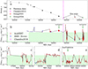 |
Fig. 1. Top: Evolution of the pulse period over time (see Sect. 3.2 for details). The dotted line represents a three-piece broken curve approximation of the data points. The dashed magenta line marks the transition to the equilibrium state. Middle: Long-term 0.5−10 keV light curve of J1301. Bottom: Zoomed-in view of segments of the long-term light curve after the transition. The light green zone indicates a flux range lower than the pre-transition quiescent flux. Green arrows indicate the times of the NuSTAR observations. |
The event data were processed to extract the light curves. First, the event files were barycenter-corrected using barycorr, then light curve extraction was performed using xselect, where a 50″ region filter was applied and a bin size of 5.0 s was set. The extracted light curves were then combined into two groups using lcurve in order to detect periodicities: Group2021 (ObsID 00095944010-22) and Group2024 (00097781001, NuSTAR2024, and 00097781004-6) containing the NuSTAR observation (see Table 1). For joint timing analysis (search for periodicities using χ2 distributions and pulse profile construction) with Swift observations, the count rates for NuSTAR2024 were adjusted by applying a conversion factor of 0.3283, representing the ratio between NuSTAR (3−79 keV) and Swift/XRT (0.2−10 keV) count rates. This factor was obtained using WebPIMMS3 based on the spectral parameters for J1301 (see Table 2).
Pulse period measurements obtained in this work.
Spectral parameters of J1301 from NuSTAR2024 data.
2.4. Chandra
During Chandra (Weisskopf et al. 2000) observations of NuSTAR’s serendipitous sources near the Galactic plane, J1301 was covered by one of the Chandra pointings (ObsID 18087, hereafter Chandra2016) on 2016 May 3 with a 9.8 ks exposure (Tomsick et al. 2018). The data were analyzed with CIAO (Chandra Interactive Analysis of Observations) v.4.16, using calibration files from CALDB v.4.11.5. A barycentric correction was applied using axbary to correct the photon arrival times. Light curves were extracted with dmextract using 35″ source and 90″ background circular regions, with a time binning of 3.3 s. Spectral extraction was performed using the specextract procedure.
2.5. Spectral data approximation
The resulting spectra of the source from all instruments were re-binned to have at least one count per energy bin using grppha utility and fitted using W-statistics4 (Wachter et al. 1979) in the XSPEC v.12.14.0h package (Arnaud 1996). All errors are given at 1σ confidence level unless otherwise specified. All quoted fluxes in this paper are unabsorbed fluxes, unless explicitly stated otherwise. This applies to values reported in Figs. 1 and 2, Tables 1 and 2, and throughout the text.
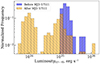 |
Fig. 2. Histogram of the luminosity distribution before and after the transition to equilibrium for Swift/XRT, Chandra, and XMM-Newton observations. Fluxes were converted to luminosities assuming a distance of 5.4 kpc. |
3. Results
3.1. Long-term light curve
To construct the long-term light curve, Swift/XRT, XMM-Newton, and Chandra observations were fitted with a simple absorbed power-law model tbabs × po, where the hydrogen column density NH was frozen at 2.48 × 1022 cm−2 (Chernyakova et al. 2005). This choice was made due to the relatively low quality of individual spectra, which did not allow us to reliably constrain NH for each observation separately. The long-term behavior of J1301 shows highly unusual activity for a BeXRB system.
Between MJD 51000 and 53000, J1301 maintained a stable flux, with the exception of a single outburst (Chernyakova et al. 2005). However, following the Chandra2016 observation (marked by the dashed magenta line in Fig. 1), J1301 began to display behavior atypical for BeXRBs: flux in the 0.5−10 keV range, which was normally around (2 − 4)×10−11 erg s−1 cm−2 during the quiescent state, dropped to a few × 10−12 erg s−1 cm−2 on multiple occasions for extended periods. This indicated the emergence of a new stable state for J1301, at a luminosity about ten times lower than the previously identified quiescent level (see the light green stripe in Fig. 1). Hereafter, we refer to this state as the “lowest” state.
To investigate in more detail the change in variability before and after the Chandra2016 (MJD 57511) observation in greater detail, we constructed a histogram of the flux frequency, as shown in Fig. 2. The histogram shows the distribution of the number of observations as a function of flux before and after MJD 57511. The data were divided into two intervals: observations taken before and after this date. Each dataset was normalized separately by dividing the number of observations in each flux bin by the total number of observations across all flux bins in a given interval. This normalization enables a clearer comparison between the two intervals.
Before the transition, the fluxes clustered around luminosities of ∼1035 erg s−1 in the 0.5−10 keV range. After the transition, a second cluster emerged at luminosities around ∼1034 erg s−1, indicating the presence of a new, lower stable state. Additionally, four significant outbursts were observed around 57850, 60470, 60560, and 60650, as shown in Fig. 1. Three consecutive outbursts around MJD 60470, 60560, and 60650 suggest the presence of an orbital period, Porb, of about 90 days. However, due to the low data quality, we do not have a high degree of confidence in this interpretation. If confirmed, though, this period would place J1301 among other BeXRBs on the Corbet (1986)Pspin − Porb diagram.
To investigate whether the newly observed low-luminosity state is caused by increased absorption rather than intrinsic flux variations, we analyzed the broadband (0.5−79 keV) spectral properties of the source in both high (∼10−11 erg s−1 cm−2) and low (∼10−12 erg s−1 cm−2) flux states. This broader energy range provides better constraints on NH compared to the 0.5−10 keV range. Specifically, we tested whether the hydrogen column density NH might be significantly higher than the previously assumed value of NH = 2.48 × 1022 cm−2 from Chernyakova et al. (2005). The measured NH in the low-luminosity state, NH = (2.4 ± 0.6)×1022 cm−2 (using the cutoffpl model) or  cm−2 (using the comptt+comptt model), as listed in Table 2, remains consistent with the previously reported value within uncertainties. This confirms that the observed flux variations are not driven by changes in absorption but rather reflect intrinsic variations in the system’s accretion rate.
Thus, after the Chandra2016 observation, the dynamic range of J1301 expanded significantly, spanning two orders of magnitude, with the new low state at the flux level of ∼10−12 erg s−1 cm−2 and new outburst flux reaching up to ∼10−10 erg s−1 cm−2. Crucially, rather than fading smoothly to a lower accretion level or displaying fast random variability, J1301 now switches between two well-defined accretion states, spending extended periods at both luminosities, ∼1035 erg s−1 and ∼1034 erg s−1. This clear bimodal behavior, in which the source oscillates between two stable luminosity states, suggests a change in its accretion regime after the Chandra2016 observation. Such a bimodal behavior has so far never been observed in other BeXRBs, making J1301 currently a unique system (see Sect. 4.1 for a further discussion).
3.2. Timing analysis
To obtain more details about the transition to a new accretion mode, we studied the rotational evolution of the XRP after this transition. For this purpose, we utilized the Chandra2016, Group2021, and Group2024 light curves; the last was obtained when J1301 was in the lowest state.
To search for periodicities, we applied the epoch-folding technique, implemented in the efsearch utility from the XRONOS package. We successfully detected the presence of pulsations with high significance in all three observations (see Table 1 and Fig. 3). The uncertainty of the period was estimated by simulating a large number of light curves, where the source count rate CR varied within the statistical error ERR: CRsim = CR + ERR × RAND([ − 1, 1]). For all simulated light curves, the pulse periods were measured to construct a distribution of their values. The mean of this distribution was taken as the final period for a given observation, and the standard deviation was used as uncertainty (see Boldin et al. 2013, for more details).
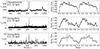 |
Fig. 3. Left: χ2 periodograms for Chandra2016 (top panel), Group2021 (middle panel), and Group2024 (bottom panel). Right: Normalized pulse profiles of J1301 for the corresponding intervals (see Sect. 3.2). |
The spin period Pspin evolution of J1301 is presented in the upper panel of Fig. 1. As shown in the figure, after a long period of stable spin-up, it ceased around MJD 57500 (Chandra2016). After this, the spin period remained constant up to MJD 60500 (Group2024), with its derivative being −8.5 × 10⁻⁸ < Ṗ < 1.2 × 10⁻⁸ s s−1. It is evident from the magenta line in Fig. 1 that the abrupt change in the long-term light curve of J1301 coincided with the cessation of spin-up.
We also constructed pulse profiles for the Chandra2016, Group2021, and Group2024 observations. The Chandra2016 and Group2021 profiles demonstrate single-peaked shapes similar to those reported by Chernyakova et al. (2005) and Krivonos et al. (2015), all at a flux level of ∼10−11 erg s−1 cm−2 (0.5−10 keV). Group2021 also exhibits a peculiar feature in phases 0.80−0.95. The pulse profile of Group2024, which includes the NuSTAR2024 observation and Swift observations at the new low state ∼10−12 erg s−1 cm−2, demonstrates a single-peaked shape, similar to other observations at higher fluxes. The pulse profiles are shown in Fig. 3, and the fluxes were normalized by their mean values.
3.3. Spectral analysis
The new lowest accretion state, characterized by luminosities ten times lower than those previously considered quiescent, is of particular interest. Figure 4 presents the phase-averaged energy spectrum of J1301 in this state. The NuSTAR2024 spectral data (FPMA and FPMB modules) were simultaneously fitted with data from the Swift/XRT telescope in PC mode to extend the energy range. To improve the statistical quality of the fit, Swift observations from 2024 July 15 to 20 (ObsIDs 00097301021, 00097781001, 00097781003, 00097781004, 00016683005, and 00097301022), which were taken close to the time of NuSTAR2024 and exhibited similar flux levels, were combined into a single spectrum.
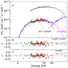 |
Fig. 4. Unfolded spectrum of J1301. Red and black dots are for the FPMA and FPMB telescopes of the NuSTAR observatory (NuSTAR2024), green for the Swift/XRT telescope. Gray dots represent NuSTAR2014 observation (Krivonos et al. 2015). The solid blue line in panel a shows the comptt+comptt spectral model, while the dashed blue lines represent the two components separately. The dashed magenta line shows the best fit with the absorbed cutoff power-law model. A blackbody model with temperature T = 1.0 keV is plotted as a dashed gray line for visual comparison. Panels b and c show the residuals for the comptt+comptt and cutoffpl continuum models, respectively. |
First we tried to describe the XRP’s spectrum in this state by a standard absorbed power law with an exponential cutoff model: tbabs × cutoffpl. The results of the spectral fit are presented in Table 2. The tbabs component models photo-absorption using abundances from Wilms et al. (2000). To account for the non-simultaneity of the observations and potential calibration discrepancies between FPMA, FPMB, and XRT, cross-calibration multiplicative factors were applied using the const model.
The spectrum is broad, significantly broader than a blackbody (see the blackbody spectrum of temperature kT = 1 keV in Fig. 4). The bolometric luminosity (0.5−100 keV) was determined to be (0.6 − 2.4)×1034 erg s−1, assuming a distance range of 3.9−7.9 kpc.
However, at energies above 20 keV, the residuals of the spectrum exhibit a wavelike structure (see Fig. 4c). The shape of the spectrum itself shows a deviation from a smooth form around 20 keV, which was not observed in higher luminosity states. Such a behavior is typical when the spectrum has a double-humped shape, commonly seen when the XRP’s luminosity falls within the 1034 − 1036 erg s−1 range (see, e.g., GX 304−1; Tsygankov et al. 2019a). To account for this, we used the two-component Comptonization spectral model comptt+comptt (Titarchuk 1994), which had previously been applied to similar XRP spectra (e.g., X Persei, Doroshenko et al. 2012; GX 304−1, Tsygankov et al. 2019a; A 0535+262, Tsygankov et al. 2019b; KS 1947+300, Doroshenko et al. 2020; SRGA J124404.1−632232, Doroshenko et al. 2022; GRO J1008−57, Lutovinov et al. 2021; RX J0440.9+4431, Salganik et al. 2023).
The peaks of the comptt+comptt model, located at approximately 10 keV and 70 keV (plasma temperatures of  keV and
  keV, respectively), align well with the typical positions of the soft (≤10 keV) and hard (≥20 keV) humps observed in other XRPs. The optical depth of the high-energy hump was fixed at τ = 100 because it could not be constrained (see the references above). The temperatures of the seed photons, T0, for the two humps were set equal to each other. The bolometric luminosity obtained using this model is slightly higher than that estimated with the cutoffpl continuum model:
  erg s−1.
None of the continuum models showed a significant detection of the Fe Kα line, reported at higher luminosities (Krivonos et al. 2015). The 3σ upper limit on the photon number flux for a narrow iron line (σ = 0.1 keV) at 6.4 keV is Firon = 1.8 × 10⁻⁶ photon cm−2 s−1, corresponding to an equivalent width of < 0.12 keV for the double Comptonization model. No CRSFs are required for the spectrum description in either of the models. The measured neutral hydrogen column density NH is consistent with the value observed at higher fluxes, 2.48 × 1022 cm−2 from Chernyakova et al. (2005).
4. Discussion
Our study of J1301 has revealed intriguing changes in its timing and spectral properties. After a long-term spin-up, the source has transitioned to an equilibrium state, marking a significant shift in its accretion behavior. This transition coincided with the emergence of a new low-luminosity accretion regime at Lbol ∼ 1034 erg s−1, an order of magnitude lower than its previously known quiescent state. The source now exhibits bimodal accretion behavior, switching between two stable luminosity states. In this newly identified low state, the spectral shape of J1301 has also changed, developing a two-hump structure instead of the typical cutoff power-law spectrum observed at higher luminosities. Additionally, the pulsations were detected in this new low state. Below, we discuss the implications of these findings, including estimates of the neutron star magnetic field and the nature of this previously unobserved accretion state.
4.1. A new low-luminosity state in J1301 and bimodal accretion
One of the key findings of this study is the identification of an accretion state at Lbol ∼ 1034 erg s−1, a new for this source (see Sect. 3.1), and an order of magnitude lower than the previously recognized quiescent luminosity of ∼1035 erg s−1 (Chernyakova et al. 2005; Krivonos et al. 2015). This newly discovered state appears to be quite stable, with the source remaining in it for prolonged time periods. However, J1301 occasionally transitions back to the level of Lbol ∼ 1035 erg s−1, demonstrating a well-pronounced bimodal flux distribution. One of these transitions appears to exhibit the classical fast-rise exponential-decay outburst profile characteristic of X-ray binaries, as observed at MJD 60471 (see Fig. 1e). Other transitions were characterized by a sharp rise and decline, as seen at MJD 58044 and 59280 (see Figs. 1c,d). Particularly interesting is that the transition from a luminosity state of ∼1035 erg s−1 to ∼1034 erg s−1 on MJD 58044 occurred in less than 2.3 days. Such rapid drops in luminosity are characteristic of the transition to the propeller regime in XRPs (see Tsygankov et al. 2016, for the cases of 4U 0115+63 and V 0332+53). However, the Group2024 observations were conducted during this newly identified low-luminosity state, where the detection of pulsations provided clear evidence of ongoing accretion. This conclusion is further supported by the observed two-humped spectral shape, consistent with theoretical predictions for low-level accretion (see Sect. 4.2 and Sokolova-Lapa et al. 2021; Mushtukov et al. 2021). Thus, these findings definitively rule out the possibility of J1301 transitioning to the propeller regime.
This new state is highly unusual when compared to classical XRP behavior and reveals a previously unexplored phenomenon. The typical behavior of long-period BeXRBs is characterized by a stable low-luminosity state at 1034 − 1035 erg s−1 (the cold-disk accretion regime; see Tsygankov et al. 2017) accompanied by periodic Type I outbursts and occasional giant Type II outbursts. In contrast, the behavior observed here departs from this norm, exhibiting no stable state and instead featuring abrupt transitions between luminosity levels of 1034 and 1035 erg s−1.
Given the atypical nature of these transitions, it is worth considering whether this behavior is an intrinsic peculiarity of J1301 or if it has gone unnoticed in other BeXRBs. Many persistent BeXRBs exhibit long pulse periods and low X-ray luminosities, making them difficult targets for frequent monitoring. The identification of a previously unknown accretion regime in J1301 raises the possibility that similar transitions could be occurring in other sources but have not been detected due to limited observational coverage. A systematic, high-cadence monitoring program for other persistent BeXRBs would be required to determine how common such a bimodal accretion behavior is.
4.2. Two-hump spectral shape
Previous observations of J1301 at luminosities in the range of Lbol ∼ 1035 − 1036 erg s−1 have shown that its spectrum is best described by a power-law continuum with an exponential cutoff at higher luminosities (Chernyakova et al. 2005; Krivonos et al. 2015), which is typical for accreting XRPs (Coburn et al. 2002; Filippova et al. 2005). However, the NuSTAR2024 observation, conducted at a significantly lower luminosity of  erg s−1, reveals a marked change in the spectral shape. Specifically, the observed spectrum is best described by a two-hump Comptonization model (see Sect. 3.3), which includes an additional high-energy component not accounted for by the cutoff power-law model. This shift from a cutoff power-law spectrum at higher luminosities to a two-hump structure at lower luminosities is consistent with broadband observations of similar spectral transitions in other long-period XRPs, such as GX 304−1 (Tsygankov et al. 2019a), A 0535+262 (Tsygankov et al. 2019b), and GRO J1008−57 (Lutovinov et al. 2021).
The two-hump spectral shape observed at low luminosities cannot be explained by the standard spectral models used for higher accretion rates. The hard X-ray component emerging at low mass accretion rates may result from cyclotron emission reprocessed by magnetic Compton scattering, while the soft component likely originates from Comptonized thermal radiation (Sokolova-Lapa et al. 2021; Mushtukov et al. 2021). Additionally, resonant scattering of photons by hot electrons leads to Doppler shifts in photon energies within the Doppler core of the CRSF. As a result, many photons escape the atmosphere through the wings of the line, where the cross section is lower, forming the observed high-energy component. Consequently, the CRSF appears near the peak of the high-energy hump (as seen in A 0535+262; Tsygankov et al. 2019b).
Based on this, the estimated magnetic field strength is ≳1013 G. However, this whole picture depends on the assumption that the two-hump spectral model accurately describes accretion at these low luminosities. If this model turns out to be oversimplified or if CRSF forms differently in this regime, then our magnetic field estimate could be off. Future hard X-ray observations extending beyond NuSTAR’s range will be needed in order to test this interpretation.
4.3. Transition to the equilibrium state
According to the current understanding of the rotational evolution of XRPs, stably accreting XRPs eventually achieve a balance between spin-up and spin-down torques, leading to what is known as the equilibrium period. As discussed in Sect. 3.2, following a 20-year-long spin-up phase, J1301 has entered an ongoing 8-year phase of a stable spin period, marked by a significant change in its long-term light curve behavior.
This transition clearly indicates that the source has reached the equilibrium state, allowing us to estimate the neutron star’s magnetic field by considering the observed spin period after the transition as the equilibrium period (Peq ≈ 634 s). We applied the accretion disk scenario (see, e.g., Chapter 5 in Lipunov 1992) with fastness parameter ωs = 0.35 (Ghosh & Lamb 1979):
 (1)
(1)
However, it is important to note that the Ghosh & Lamb model, while widely used, has known limitations and uncertainties. The model relies on assumptions about the disk-magnetosphere interaction that may not fully capture the complexities of real accretion processes. For example, the model assumes significant field penetration into the disk, which may be unrealistic due to high disk conductivity (see Lai 2014, for a review). It was also suggested that the accretion flow in strongly magnetized neutron stars may differ significantly from the classical Ghosh & Lamb picture, with alternative models proposing a smaller magnetospheric radius and different torque contributions (Wang 1995; Bozzo et al. 2018). Thus, while Eq. (1) provides a useful framework for interpreting our results, the inferred values should be considered approximate and subject to the theoretical uncertainties.
Using the average 0.5−10 keV luminosity after the transition to equilibrium, Leq = (4 − 17)×1034 erg s−1 (taking into account uncertainties in a distance of  kpc), we estimate the magnetic field strength to be B ≈ (6 − 12)×1013 G. This value is in good agreement with the estimate derived from the power spectrum break frequency, as detailed in Appendix A, and also consistent with the magnetic field strength inferred from the observed two-hump spectral shape, which suggests B ≳ 1013 G (see Sect. 4.2).
5. Conclusions
We have analyzed the long-term behavior of the Be/X-ray pulsar J1301, focusing on its transition to the equilibrium state. The data from the NuSTAR, Swift, XMM-Newton, and Chandra observatories were used to investigate changes in the XRP’s timing and spectral characteristics.
We were able to establish the presence of pulsations in three observations, on MJD 57511.4–57511.6, 59285.6–59309.2, and 60507.3–60520.0, demonstrating that after more than 20 years of continuous spin-up, J1301 has reached a stable spin period (Peq) of approximately 634 s, indicating a shift to an equilibrium state. All three observations have single-peaked pulse profiles. This transition coincided with the emergence of a previously unknown low-luminosity accretion regime at Lbol ∼ 1034 erg s−1, an order of magnitude lower than its previously known quiescent state. Additionally, we find tentative evidence of an orbital period of ≈90 days based on three consecutive outbursts around MJD 60470, 60560, and 60650.
The source exhibited behavior atypical for BeXRBs, occasionally transitioning between these two stable luminosity levels of approximately 1034 erg s−1 and 1035 erg s−1 and remaining in both states for extended periods (i.e., it exhibited a well-pronounced bimodal behavior). The transition from 1035 erg s−1 to 1034 erg s−1 occurred in less than 2.3 days which is the interval between consecutive observations, though the transition itself may have taken an even shorter time. This behavior could indicate a transition to the propeller regime. However, timing analysis of this state confirmed the presence of pulsations, and spectral analysis revealed a two-hump Comptonization shape, in contrast to the cutoff power-law spectrum observed at higher luminosities. The detection of pulsations and the two-hump spectral shape rules out the possibility of a propeller regime in this newly identified state. The mechanism driving the transition to this previously unknown accretion regime remains unclear. However, the identification of a bimodal accretion behavior in J1301 suggests that similar transitions can occur in other sources but have remained undetected due to limited observational coverage.
Despite the absence of CRSF detection in the spectrum, we estimated the magnetic field strength using the equilibrium spin period value and the perturbation propagation model. In these two estimations, the magnetic field was on the order of ≃1013 − 1014 G, which agrees well with the observed spectral shape in the low state. We note that for such a strong magnetic field, CRSF should indeed not be observable in the NuSTAR energy range.
However, it is important to note that these estimates are strongly model-dependent and subject to significant uncertainties. Future observations, particularly in a broader X-ray energy range, will be crucial for refining these estimates and further understanding the accretion mechanisms in this system.
Acknowledgments
AS acknowledges support from the EDUFI Fellowship and Jenny and Antti Wihuri Foundation. DM acknowledge support by the state of Baden-Württemberg through bwHPC. We are grateful to the Swift team for approving and rapid scheduling of the monitoring campaign. We are grateful to the NuSTAR team for approving and rapid scheduling of the observation. This work made use of data supplied by the UK Swift Science Data Centre at the University of Leicester and data obtained with NuSTAR mission, a project led by Caltech, funded by NASA, and managed by JPL. This research also has made use of the NuSTAR Data Analysis Software (NUSTARDAS) jointly developed by the ASI Science Data Centre (ASDC, Italy) and Caltech. This research has made use of data and software provided by the High Energy Astrophysics Science Archive Research Centre (HEASARC), which is a service of the Astrophysics Science Division at NASA/GSFC and the High Energy Astrophysics Division of the Smithsonian Astrophysical Observatory. This research is based on observations obtained with XMM-Newton, an ESA science mission with instruments and contributions directly funded by ESA Member States and NASA. The scientific results reported in this article are based in part of data obtained from the Chandra Data Archive.
References
- Arnaud, K. A. 1996, ASP Conf. Ser., 101, 17 [Google Scholar]
- Bailer-Jones, C. A. L., Rybizki, J., Fouesneau, M., Demleitner, M., & Andrae, R. 2021, AJ, 161, 147 [Google Scholar]
- Bird, A. J., Barlow, E. J., Bassani, L., et al. 2006, ApJ, 636, 765 [NASA ADS] [CrossRef] [Google Scholar]
- Boldin, P. A., Tsygankov, S. S., & Lutovinov, A. A. 2013, Astron. Lett., 39, 375 [NASA ADS] [CrossRef] [Google Scholar]
- Bozzo, E., Ascenzi, S., Ducci, L., et al. 2018, A&A, 617, A126 [NASA ADS] [EDP Sciences] [Google Scholar]
- Burrows, D. N., Hill, J. E., Nousek, J. A., et al. 2005, Space Sci. Rev., 120, 165 [Google Scholar]
- Chernyakova, M., Shtykovsky, P., Lutovinov, A., et al. 2004, ATel, 251, 1 [Google Scholar]
- Chernyakova, M., Lutovinov, A., Rodríguez, J., & Revnivtsev, M. 2005, MNRAS, 364, 455 [NASA ADS] [CrossRef] [Google Scholar]
- Coburn, W., Heindl, W. A., Rothschild, R. E., et al. 2002, ApJ, 580, 394 [NASA ADS] [CrossRef] [Google Scholar]
- Coleiro, A., Chaty, S., Zurita Heras, J. A., Rahoui, F., & Tomsick, J. A. 2013, A&A, 560, A108 [NASA ADS] [CrossRef] [EDP Sciences] [Google Scholar]
- Corbet, R. H. D. 1986, MNRAS, 220, 1047 [NASA ADS] [CrossRef] [Google Scholar]
- Doroshenko, V., Santangelo, A., Kreykenbohm, I., & Doroshenko, R. 2012, A&A, 540, L1 [NASA ADS] [CrossRef] [EDP Sciences] [Google Scholar]
- Doroshenko, R., Piraino, S., Doroshenko, V., & Santangelo, A. 2020, MNRAS, 493, 3442 [NASA ADS] [CrossRef] [Google Scholar]
- Doroshenko, V., Staubert, R., Maitra, C., et al. 2022, A&A, 661, A21 [NASA ADS] [CrossRef] [EDP Sciences] [Google Scholar]
- Evans, P. A., Beardmore, A. P., Page, K. L., et al. 2009, MNRAS, 397, 1177 [Google Scholar]
- Ferrigno, C., Farinelli, R., Bozzo, E., et al. 2013, A&A, 553, A103 [NASA ADS] [CrossRef] [EDP Sciences] [Google Scholar]
- Filippova, E. V., Tsygankov, S. S., Lutovinov, A. A., & Sunyaev, R. A. 2005, Astron. Lett., 31, 729 [NASA ADS] [CrossRef] [Google Scholar]
- Gabriel, C., Denby, M., Fyfe, D. J., et al. 2004, ASP Conf. Ser., 314, 759 [Google Scholar]
- Gehrels, N., Chincarini, G., Giommi, P., et al. 2004, ApJ, 611, 1005 [Google Scholar]
- Ghosh, P., & Lamb, F. K. 1979, ApJ, 234, 296 [Google Scholar]
- Harrison, F. A., Craig, W. W., Christensen, F. E., et al. 2013, ApJ, 770, 103 [Google Scholar]
- Illarionov, A. F., & Sunyaev, R. A. 1975, A&A, 39, 185 [NASA ADS] [Google Scholar]
- Krivonos, R. A., Tsygankov, S. S., Lutovinov, A. A., et al. 2015, ApJ, 809, 140 [NASA ADS] [CrossRef] [Google Scholar]
- Lai, D. 2014, EPJ Web Conf., 64, 01001 [NASA ADS] [CrossRef] [EDP Sciences] [Google Scholar]
- Lipunov, V. M. 1992, Astrophysics of Neutron Stars (Berlin, Heidelberg: Springer) [CrossRef] [Google Scholar]
- Lutovinov, A., Tsygankov, S., & Chernyakova, M. 2012, MNRAS, 423, 1978 [NASA ADS] [CrossRef] [Google Scholar]
- Lutovinov, A., Tsygankov, S., Molkov, S., et al. 2021, ApJ, 912, 17 [Google Scholar]
- Lyubarskii, Y. E. 1997, MNRAS, 292, 679 [Google Scholar]
- Masetti, N., Pretorius, M. L., Palazzi, E., et al. 2006, A&A, 449, 1139 [NASA ADS] [CrossRef] [EDP Sciences] [Google Scholar]
- Mönkkönen, J., Tsygankov, S. S., Mushtukov, A. A., et al. 2019, A&A, 626, A106 [NASA ADS] [CrossRef] [EDP Sciences] [Google Scholar]
- Mönkkönen, J., Tsygankov, S. S., Mushtukov, A. A., et al. 2022, MNRAS, 515, 571 [Google Scholar]
- Mushtukov, A., & Tsygankov, S. 2024, Handbook of X-ray and Gamma-ray Astrophysics (Singapore: Springer), 4105 [CrossRef] [Google Scholar]
- Mushtukov, A. A., Suleimanov, V. F., Tsygankov, S. S., & Portegies Zwart, S. 2021, MNRAS, 503, 5193 [Google Scholar]
- Nakajima, M., Negoro, H., Mihara, T., et al. 2019, IAU Symp., 346, 131 [Google Scholar]
- Reig, P. 2011, Ap&SS, 332, 1 [Google Scholar]
- Reig, P., & Roche, P. 1999, MNRAS, 306, 100 [NASA ADS] [CrossRef] [Google Scholar]
- Revnivtsev, M. G., Sazonov, S. Y., Molkov, S. V., et al. 2006, Astron. Lett., 32, 145 [NASA ADS] [CrossRef] [Google Scholar]
- Revnivtsev, M., Churazov, E., Postnov, K., & Tsygankov, S. 2009, A&A, 507, 1211 [CrossRef] [EDP Sciences] [Google Scholar]
- Salganik, A., Tsygankov, S. S., Doroshenko, V., et al. 2023, MNRAS, 524, 5213 [NASA ADS] [CrossRef] [Google Scholar]
- Sokolova-Lapa, E., Gornostaev, M., Wilms, J., et al. 2021, A&A, 651, A12 [NASA ADS] [CrossRef] [EDP Sciences] [Google Scholar]
- Titarchuk, L. 1994, ApJ, 434, 570 [NASA ADS] [CrossRef] [Google Scholar]
- Tomsick, J. A., Lansbury, G. B., Rahoui, F., et al. 2018, ApJ, 869, 171 [Google Scholar]
- Tsygankov, S. S., Lutovinov, A. A., Doroshenko, V., et al. 2016, A&A, 593, A16 [NASA ADS] [CrossRef] [EDP Sciences] [Google Scholar]
- Tsygankov, S. S., Mushtukov, A. A., Suleimanov, V. F., et al. 2017, A&A, 608, A17 [NASA ADS] [CrossRef] [EDP Sciences] [Google Scholar]
- Tsygankov, S. S., Rouco Escorial, A., Suleimanov, V. F., et al. 2019a, MNRAS, 483, L144 [NASA ADS] [CrossRef] [Google Scholar]
- Tsygankov, S. S., Doroshenko, V., Mushtukov, A. A., et al. 2019b, MNRAS, 487, L30 [NASA ADS] [CrossRef] [Google Scholar]
- Wachter, K., Leach, R., & Kellogg, E. 1979, ApJ, 230, 274 [NASA ADS] [CrossRef] [Google Scholar]
- Wang, Y. M. 1995, ApJ, 449, L153 [NASA ADS] [Google Scholar]
- Weisskopf, M. C., Tananbaum, H. D., Van Speybroeck, L. P., & O’Dell, S. L. 2000, Proc. SPIE, 4012, 2 [Google Scholar]
- Wilms, J., Allen, A., & McCray, R. 2000, ApJ, 542, 914 [Google Scholar]
Appendix A: Disk truncation
The light curves of XRPs exhibit both periodic and aperiodic variability. A widely accepted model for describing the aperiodic variability is the “perturbation propagation” model (Lyubarskii 1997). In this model, variations in X-ray brightness are attributed to fluctuations in the mass accretion rate on Keplerian timescales, driven by the multiplicative superposition of stochastic perturbations within the accretion flow. These perturbations originate from viscous stresses at different radii in the disk. When integrated, the resulting variability produces a characteristic red noise with a power-law power spectrum.
The power spectrum P(f) breaks at the break frequency fbr, which corresponds to the Keplerian frequency νK at the inner disk radius. As a result, below fbr, P(f)∝f−1 (Lyubarskii 1997), and at higher Fourier frequencies, the spectrum is P(f)∝f−2. Measurement of the break frequency allows the estimation of the inner disk radius (Rin) and thus the magnetic field (Revnivtsev et al. 2009):
 (A.1)
(A.1)
We assume Rin to be equal to the magnetospheric radius Rm, which can be related to the luminosity and the magnetic field strength as (e.g., Mushtukov & Tsygankov 2024)
 (A.2)
(A.2)
where mNS = MNS/M⊙, L37 is the luminosity in units of 1037 erg s−1, R6 is the neutron star radius in 106 cm, and B12 is the neutron star magnetic field in 1012 G. The coefficient Λ relates the Alfvén radius to the magnetospheric radius Rm = ΛRA. For accretion from a gas pressure-dominated disk, this coefficient is typically taken to be Λ = 0.5 (Ghosh & Lamb 1979).
Based on the study of J1301 using NuSTAR2014 data, Krivonos et al. (2015) measured the break frequency fbr = 0.0066 Hz in the power spectrum at a bolometric flux of 1.2 × 10⁻¹⁰ erg s−1 cm−2 (calculated based on spectral parameters from Krivonos et al. 2015). From Eqs. (A.1) and (A.2), we estimate the magnetic field to be B≈(5–11)×1013 G assuming canonical neutron star mass M = 1.4 M⊙ and radius R = 12 km.
The identification of the break frequency fbr with the Keplerian frequency at the magnetospheric radius is not firmly established and remains a subject of debate (see, e.g., Mönkkönen et al. 2019, 2022). While this assumption is commonly used, the exact origin of the broad-band noise in power spectra is not fully understood, and alternative interpretations exist. Additionally, the relation between fbr and the inner disk radius may be influenced by factors beyond magnetic truncation, such as local disk instabilities or other accretion flow properties. In light of these uncertainties, estimates of the neutron star’s magnetic field based on fbr should be treated with caution, as they may be subject to systematic uncertainties arising from these alternative influences.
Appendix B: Observation log
XMM-Newton and Swift/XRT observations used in this work can be found in Tables B.1 and B.2.
XMM-Newton observations used in this work.
Swift/XRT observations used in this work.
All Tables
All Figures
|
Fig. 1. Top: Evolution of the pulse period over time (see Sect. 3.2 for details). The dotted line represents a three-piece broken curve approximation of the data points. The dashed magenta line marks the transition to the equilibrium state. Middle: Long-term 0.5−10 keV light curve of J1301. Bottom: Zoomed-in view of segments of the long-term light curve after the transition. The light green zone indicates a flux range lower than the pre-transition quiescent flux. Green arrows indicate the times of the NuSTAR observations. |
| In the text | |
|
Fig. 2. Histogram of the luminosity distribution before and after the transition to equilibrium for Swift/XRT, Chandra, and XMM-Newton observations. Fluxes were converted to luminosities assuming a distance of 5.4 kpc. |
| In the text | |
|
Fig. 3. Left: χ2 periodograms for Chandra2016 (top panel), Group2021 (middle panel), and Group2024 (bottom panel). Right: Normalized pulse profiles of J1301 for the corresponding intervals (see Sect. 3.2). |
| In the text | |
|
Fig. 4. Unfolded spectrum of J1301. Red and black dots are for the FPMA and FPMB telescopes of the NuSTAR observatory (NuSTAR2024), green for the Swift/XRT telescope. Gray dots represent NuSTAR2014 observation (Krivonos et al. 2015). The solid blue line in panel a shows the comptt+comptt spectral model, while the dashed blue lines represent the two components separately. The dashed magenta line shows the best fit with the absorbed cutoff power-law model. A blackbody model with temperature T = 1.0 keV is plotted as a dashed gray line for visual comparison. Panels b and c show the residuals for the comptt+comptt and cutoffpl continuum models, respectively. |
| In the text | |
Current usage metrics show cumulative count of Article Views (full-text article views including HTML views, PDF and ePub downloads, according to the available data) and Abstracts Views on Vision4Press platform.
Data correspond to usage on the plateform after 2015. The current usage metrics is available 48-96 hours after online publication and is updated daily on week days.
Initial download of the metrics may take a while.