| Issue |
A&A
Volume 696, April 2025
|
|
|---|---|---|
| Article Number | A114 | |
| Number of page(s) | 17 | |
| Section | Numerical methods and codes | |
| DOI | https://doi.org/10.1051/0004-6361/202453314 | |
| Published online | 11 April 2025 | |
Radio pulsar population synthesis with consistent flux measurements using simulation-based inference
1
Institute of Space Sciences (CSIC-ICE),
Campus UAB, Carrer de Can Magrans s/n,
08193
Barcelona, Spain
2
Institut d’Estudis Espacials de Catalunya (IEEC),
Carrer Gran Capità 2–4,
08034
Barcelona, Spain
3
Department of Physics, Royal Holloway, University of London,
Egham,
TW20 0EX,
UK
★ Corresponding author; pardo@ice.csic.es
Received:
5
December
2024
Accepted:
25
February
2025
The properties of isolated Galactic radio pulsars can be inferred by modelling their evolution, from birth to the present, through pulsar population synthesis. This involves simulating a mock population, applying observational filters, and comparing the resulting sources to the limited subset of detected pulsars. We specifically focus on the magneto-rotational properties of Galactic isolated neutron stars and provide new insights into the intrinsic radio luminosity law. To better constrain the intrinsic radio luminosity, for the first time in pulsar population synthesis studies, we incorporate data from the Thousand Pulsar Array program on MeerKAT, which contains the largest unified sample of neutron stars with consistent flux measurement to date. In particular, we employed a simulation-based inference technique called Truncated sequential neural posterior estimation (TSNPE) to infer the parameters of our pulsar population model. This technique trains a neural density estimator on simulated pulsar populations to approximate the posterior distribution of underlying parameters. This method efficiently explores the parameter space by focusing on regions most likely to match the observed data, significantly reducing the required training dataset size. We find that adding flux information as an input to the neural network significantly improves the constraints on the pulsars’ radio luminosity and improves the estimates on other input parameters. Moreover, we demonstrate the efficiency of TSNPE over standard neural posterior estimation, as we achieve robust inferences of magneto-rotational parameters consistent with previous studies while using only around 4% of the simulations required by NPE approaches.
Key words: methods: data analysis / methods: statistical / stars: neutron / pulsars: general
© The Authors 2025
 Open Access article, published by EDP Sciences, under the terms of the Creative Commons Attribution License (https://creativecommons.org/licenses/by/4.0), which permits unrestricted use, distribution, and reproduction in any medium, provided the original work is properly cited.
This article is published in open access under the Subscribe to Open model. Subscribe to A&A to support open access publication.
1 Introduction
Neutron stars are remnants of core-collapse supernovae of massive stars characterised by their extreme properties, such as their high magnetic field and rapid rotation. Originally detected in radio as pulsars, neutron stars have since been observed across the electromagnetic spectrum, from radio to gamma rays. This diverse set of observations has resulted in a wide variety of classes of neutron stars, whose many properties, such as magnetic field evolution, are still not fully understood. Among the various classes of neutron stars, radio pulsars are the most prevalent. These isolated neutron stars emit primarily in the radio band. As they rotate, their strong magnetic fields accelerate particles to relativistic speeds along open magnetic field lines, producing the characteristic beamed emission observed in pulsars (Goldreich & Julian 1969; Ruderman & Sutherland 1975). However, the precise mechanisms driving this coherent radio emission remain poorly understood (Zhang et al. 2000; Chen & Ruderman 1993). As a result, studying neutron stars not only deepens our understanding of their nature but also provides valuable insights into broader astrophysical phenomena, including core-collapse supernovae.
Pulsar population synthesis studies are a powerful tool to analyse the whole population of neutron stars. Although we expect between 106 and 108 neutron stars in our galaxy based on core-collapse supernova rates (Rozwadowska et al. 2021), only approximately 3, 000 isolated neutron stars have been detected (Manchester et al. 2005) due to observational biases. By modelling neutron stars from their birth to the present and applying observational filters, population synthesis allows us to compare the observed neutron stars with simulated populations and thus to study the properties of the whole population by looking at the small subset of detected sources. Numerous studies have applied this technique to model the Galactic neutron star population using various statistical techniques (e.g., Narayan & Ostriker 1990; Lorimer 2004; Faucher-Giguère & Kaspi 2006; Gonthier et al. 2007; Bates et al. 2014; Gullón et al. 2014, 2015; Cieślar et al. 2020). However, these studies typically rely on simplified likelihoods or metrics to compare simulations with observations, followed by methods such Markov chain Monte Carlo (MCMC) as applied in Cieślar et al. (2020) or annealing techniques (Gullón et al. 2014) for parameter estimation.
In Graber et al. (2024) (hereafter referred to as Paper I), we demonstrate that simulation-based inference (SBI; see, e.g., Cranmer et al. 2020) is an effective technique for performing inference with complex simulators, such as those modelling the evolution of the neutron star population. SBI, also known as likelihood-free inference, uses neural networks and the stochastic nature of simulators to approximate the posterior distribution without the need for a simplified likelihood model. Paper I shows the strength of this method when performing pulsar population synthesis with a realistic prescription for magnetic field decay, allowing us to infer the magnetic field and period distributions at birth.
With the future Square Kilometre Array (SKA), the number of detected pulsars in our Galaxy will increase by an order of magnitude (Dai et al. 2017), which will be crucial for deepening our understanding of the neutron star population. In particular, MeerKAT has already created the largest unified sample of neutron stars to date, including consistent flux measurements (Posselt et al. 2023). Building on the work in Paper I, we expand the methodology in the present paper by taking advantage of the new accurate flux measurements. Using the pulsar population synthesis code described below, we constrain the magnetic field and period at birth and also gain new insights into the radio luminosity law of isolated Galactic neutron stars.
In Paper I, we employed an SBI method known as Neural posterior estimation (NPE; Papamakarios & Murray 2016), which uses a neural network to directly approximate the posterior distribution of the underlying parameters. However, NPE becomes inefficient when dealing with high-dimensional parameter spaces. In this work, we address this limitation by using a more efficient algorithm called Truncated sequential neural posterior estimation (TSNPE; Deistler et al. 2022). In particular, TSNPE guides the exploration of the parameter space by using the neural network itself, making the inference process significantly more efficient. This efficiency allows us to expand the number of parameters being inferred and extend the scope of our analysis.
The paper is organized as follows: Section 2 summarises the most relevant aspects of our population synthesis framework used in this study. We then provide an overview of SBI and TSNPE in Sections 3.1 and 3.2, respectively, whereas in Sections 3.3 to 3.5, we summarise the technical aspects of TSNPE. In Section 4, we explain the experiments performed in this work. We show the results for the experiments used to test the TSNPE technique in Sections 5.1 and 5.2, while we outline the main results in Section 5.3. Finally, we provide a detailed discussion of our approach and results in Section 6.
2 Pulsar population synthesis
In this work, we focus on modelling the population of isolated rotation-powered radio pulsars. These are isolated neutron stars whose radio emissions are powered by the loss of rotational energy. We performed Monte Carlo simulations to model both the dynamical and magneto-rotational evolution of this type of neutron star, which we followed by the application of observational biases to compare the simulated populations with observations. For a detailed description of all equations and the physics underlying the simulations, we refer the reader to Paper I, though we summarise the main steps here for completeness.
2.1 Dynamical and magneto-rotational evolution
To reduce the computational cost, we took advantage of the fact that the magneto-rotational and dynamical evolution are decoupled. This allowed us to fix the parameters governing the dynamical evolution, which in turn enabled us to perform the corresponding evolution only once to generate a comprehensive database of dynamically evolved neutron stars. This database then served as the foundation for the subsequent magneto-rotational evolution.
To create the dynamically evolved database, we simulated a population of 107 neutron stars, assigning them random ages up to 108 yr to ensure a realistic detection sample, as neutron stars older than this age are no longer observable. Since we expected massive OB stars, the precursors of neutron stars, to be located in star-forming regions directly related to the distribution of free electrons, we sampled the initial positions based on the Galactic electron density distribution from Yao et al. (2017). During supernova explosions, neutron stars receive kicks as a result of asymmetries in the explosion (see Coleman & Burrows 2022; Janka et al. 2022). To model these kicks, we sample the kick velocity from a Maxwell distribution, using a fiducial value of σk ≈ 260 km s−1 for the dispersion parameter (Hobbs et al. 2005), which is broadly consistent with the observed proper motions of radio pulsars (Hobbs et al. 2005; Faucher-Giguère & Kaspi 2006). To determine the positions of neutron stars in the Galaxy at any given time, we then computed their dynamical evolution by solving the Newtonian equations of motion in Galactocentric coordinates.
Radio pulsars can be approximated as rotating magnetic dipoles, with the magnetic dipole axis misaligned with respect to the rotation axis. As neutron stars age, magnetospheric torques cause a gradual loss of rotational energy. This torque leads to a gradual slowdown in the star’s spin and drives the alignment of the magnetic and rotation axes. We simulated this magneto-rotational evolution by sampling neutron stars from our dynamical database and tracking changes in spin period, misalignment angle, and magnetic field.
We began by randomly selecting an initial misalignment angle, χ0, in the range [0, π/ 2] based on the probability distribution (Gullón et al. 2014)
 (1)
(1)
Next, we selected the initial magnetic field strength, B0 (in G), and the initial spin period, P0 (in s), for each neutron star. These parameters are drawn from normal distributions in logarithmic space defined as follows (Popov et al. 2010; Gullón et al. 2014; Igoshev 2020; Igoshev et al. 2022; Xu et al. 2023):
 (2)
(2)
 (3)
(3)
The means, µlog B, µlog P, and the standard deviations, σlog B , σlog P , are free parameters in our model.
To model the evolution of the spin period and the misalignment angle due to the loss of rotational energy via dipole radiation, we followed Philippov et al. (2014) and Spitkovsky (2006) and solved the following coupled differential equations:
 (4)
(4)
 (5)
(5)
where c is the speed of light, RNS ≈ 11 km is the neutron-star radius, and  g cm2 is the stellar moment of inertia (for a fiducial mass MNS ≈ 1.4 M⊙). For realistic pulsars surrounded by plasma-filled magnetospheres, we chose κ0 ≃ κ1 ≃ κ2 ≃ 1.
We also incorporated magnetic field decay to accurately capture the long-term magneto-rotational evolution of neutron stars. The evolution of the dipolar magnetic field strength in neutron stars is influenced by both the Hall effect and ohmic dissipation in the crust (Viganò et al. 2013). This decay is particularly significant for strongly magnetised neutron stars (fields above 1013 G), making it relevant for a considerable fraction of our simulated pulsar population. We compute the dipolar magnetic field at time t by parametrising numerical simulation obtained with the magneto-thermal code of Viganò et al. (2021). However, at late times (t > 106 yr) this numerical prescription becomes unreliable because it relies on implementations of complex microphysics that are unsuitable for cold and old stars. Instead, we modelled the evolution of the magnetic field decay at late times with a power law:
 (6)
(6)
where τlate ≈ 2 × 10⁶ yr was chosen to fit the simulations and the power-law index, alate , is an additional free parameter of our model (see Appendix A of Paper I for details). Therefore, we have a total of five free parameters related to the magneto-rotational evolution, which hereafter is referred to as the magneto-rotational parameters.
2.2 Intrinsic bolometric luminosity prescription
To compare the simulated populations with observations, it is essential to consider observational biases. We begin by computing the geometry of the radio beam to estimate how many neutron stars have radio beams that cross our line of sight (see Section 2.4 in Paper I, for details). For those neutron stars that are potentially detectable, we then compute their radio fluxes to determine if they fall within the detection limits of the modelled radio surveys. To obtain these radio fluxes, we assume that some percentage of the rotational energy, Erot, of each star is converted into coherent radio emission. Therefore, we modelled the intrinsic luminosity as being proportional to a power law of the rotational energy loss, with an exponent α:
 (7)
(7)
where L0 is a normalisation factor whose logarithm is sampled from a normal distribution with mean µlog L and standard deviation σlog L = 0.8 (see also Faucher-Giguère & Kaspi 2006; Gullón et al. 2014). Ė0,rot represents the rotational energy loss corresponding to a neutron star luminosity L0 . Although this prescription differs slightly from that of Paper I (Eq. (16)), both relate the loss of the rotational energy with the luminosity. We use this new prescription in this work to remove correlations between the power law index α and the normalisation factor L0 , which helps with the inference procedure outlined below. We choose Ė0,rot = 1029 erg s−1 to be the minimum observed value for the radio pulsar population (see Figure 3 of Posselt et al. 2023). In this work,  and α are treated as free parameters, resulting in a total of seven free parameters, including those related to the magneto-rotational evolution.
2.3 Radio survey detectability
In what follows, our inference of the luminosity parameters depends on the details of the emission geometry as well as the propagation of the radiation. We summarise our prescription here and refer the reader to Section 2.4 of Paper I for further information. In particular, once we computed the luminosity and the geometry of the beam and extracted the pulsar distances from the dynamical database, we computed the bolometric flux, S, for a given pulsar:
 (8)
(8)
where d is the distance and Ωb the solid angle covered by a pulsar’s two radio beams. To calculate the radio flux density, S f (in Jy), at a given observing frequency, f , from the bolometric flux, S, we followed the approach of Lorimer & Kramer (2012), assuming that the radio emission spectrum follows a power law in f . We note that we adopt two different spectral indices in the following: for the simulations used in the experiments constraining five model parameters, where we compare the results of this work with those of Paper I (see Section 4 below), we adopt a spectral index of −1.6 as suggested by Jankowski et al. (2018). In contrast, for experiments focused on inferring magneto-rotational and luminosity parameters by adding MeerKAT fluxes, we assume a spectral index of −1.8 based on the mean spectral index estimated by Posselt et al. (2023) (see their Figure 8) to maintain consistency. At this point, given the intrinsic pulse width wint, we can compute the fluence as S f wint. Although this fluence is conserved when the radio signal propagates towards the observer, the pulse gets broadened by dispersion and scattering caused by the free electrons and the interstellar medium. Therefore, we computed the radio fluxes reaching Earth as:
 (9)
(9)
where wobs is the observed pulse width.
In this study, we focus on three major surveys conducted with Murriyang, the Parkes radio telescope: the Parkes Multibeam Pulsar Survey (PMPS) (Manchester et al. 2001; Lorimer et al. 2006), the Swinburne Intermediate-latitude Pulsar Survey (SMPS) (Edwards et al. 2001; Jacoby et al. 2009), and the low- and mid-latitude High Time Resolution Universe (HTRU) surveys (Keith et al. 2010).
Equipped with the observed radio fluxes at the central frequency of each radio survey, we can now determine whether each pulsar in our synthetic sample is detectable by each radio survey. First, we exclude stars that do not lie within the survey’s sky coverage. Next, we computed the signal-to-noise ratio using the radiometer equation (Lorimer & Kramer 2012):
![$S/N = {{{S_{{\rm{mean}}}}G\sqrt {{n_{{\rm{pol}}}}{\rm{\Delta }}{f_{{\rm{bw}}}}{t_{{\rm{obs}}}}} } \over {\beta \left[ {{T_{{\rm{sys}}}} + {T_{{\rm{sky}}}}(l,b)} \right]}}\sqrt {{{P - {w_{{\rm{obs}}}}} \over {{w_{{\rm{obs}}}}}}} .$](/articles/aa/full_html/2025/04/aa53314-24/aa53314-24-eq12.png) (10)
(10)
Here, Smean ≃ S f,obswobs/P denotes the mean flux density averaged over a single rotation period P, G is the receiver gain (see Lorimer et al. 1993; Bates et al. 2014, for details), npol is the number of detected polarisations, Δfbw the observing bandwidth, tobs the integration time and β > 1 a degradation factor that accounts for imperfections during the digitisation of the signal. Moreover, Tsys denotes the system temperature and Tsky(l, b) is the sky background temperature dominated by synchrotron emission of Galactic electrons. Therefore, we count a pulsar as detected if its computed S/N ratio exceeds the detection threshold for that survey. A summary of all relevant survey parameters is provided in Table 1 in Paper I.
To efficiently perform the magneto-rotational evolution without assuming a fixed birth rate, we adopt the following approach: we sample a batch of 100 000 neutron stars from our dynamical database, evolve this subset magneto-rotationally, and subsequently compute their radio emission properties. We then evaluate how many of these neutron stars are detected by each survey and check if this number matches the observed population. This process is repeated until the number of detected pulsars in the simulation matches that of the observed sample for each survey. As the number of simulated detected neutron stars approaches that of the observations, we reduce the batch size to closely match the observed number of neutron stars. We note that this method allows us to estimate the birth rate at the end of each simulation by dividing the total number of neutron stars sampled from the dynamical database by the maximum age considered. The resulting output of each simulation consists of three data frames, each containing the detected neutron stars for one of the surveys.
2.4 Observed neutron star population
For the observed neutron star sample, we use the ATNF Pulsar Catalogue (Manchester et al. 2005)1, excluding extragalactic sources and those located in globular clusters. Our focus is on isolated Galactic radio pulsars, as our current model does not account for the physics involved in simulating recycled millisecond pulsars, which have undergone accretion from a companion star. Consequently, we exclude pulsars with period derivatives below Ṗ < 10−19ss−1, and P < 0.01 s to remove recycled neutron stars.
For Experiments 1 and 2 (for more details see Section 4), we employ version v1.69 of the ATNF Pulsar Catalogue as we compare our results with those from Paper I and use their training dataset. However, for Experiments 3 through 5, where we also vary the luminosity and incorporate MeerKAT flux measurements, we use the most recent version of the catalogue v2.5.1. In this updated version, the number of detected pulsars per survey, which we aim to recover in our simulations, is as follows:
 (11)
(11)
We note that even though we apply the same selection criteria to filter the observed data, the numbers of pulsars differ slightly from those reported in Paper I. The discrepancy in the number of detected sources in HTRU between this paper and Paper I is due to a bug in version v1.69 of the ATNF Pulsar Catalogue, while the difference in PMPS is due to the reprocessing of archival data from PMPS (Sengar et al. 2023). Additionally, we have updated the period values for 11 pulsars for which the ATNF Pulsar Catalogue initially reported a harmonic of the true period, following the corrections made by Song et al. (2023). For flux measurements, we use data from the Thousand Pulsar Array (TPA) program (Johnston et al. 2020), which is part of the large survey project MeerTIME on the MeerKAT telescope. The TPA provides a consistently observed sample, as the data were collected using a single telescope with similar observing parameters and processed through a standardised data reduction pipeline. Specifically, we use the flux measurements at 1.429 GHz reported by Posselt et al. (2023). Since the TPA program did not observe all pulsars detected with PMPS, SMPS, and HTRU, we compute the number of overlapping pulsars between MeerKAT and each of these surveys as follows:
 (12)
(12)
We verified that these subsets of overlapping pulsars do not show additional biases in terms of dispersion measure (DM), sky position, period, or period derivative compared to the full observed populations in the three surveys. Because the TPA program was designed to re-observe known pulsars rather than detect new ones, and TPA does not introduce any additional biases, we do not need to model a separate detection filter for the MeerKAT flux measurements. Instead, we extract a random subset of simulated neutron stars for each survey to match the number of pulsars observed by MeerKAT as listed in Eq. (12), when comparing the simulated fluxes measurements with the observed values.
2.5 Representation of simulation output
To feed the simulated neutron star population into the neural- network based SBI algorithm discussed in Section 3, we need to choose a suitable representation. For this purpose, we represent each mock simulation as six density maps: three P-Ṗ diagrams and three P-Ṗ averaged flux maps, corresponding to the three radio surveys modelled in this study. An example of these maps is shown in Figure 1. Both types of maps are P-Ṗ diagrams with parameter limits set to P ∈ [0.001, 100] s and Ṗ ∈ [10−21, 10−9] s s−1, using a resolution of 32 bins. However, they differ in terms of colour representation and the number of simulated neutron stars present. In the P-Ṗ density maps, shown in the top panels, the colour indicates the number of neutron stars in each bin, and the number of simulated neutron stars matches the total number of detected pulsars in each survey, as listed in Eq. (11). On the other hand, the P-Ṗ averaged flux maps, shown in the bottom panels, represent the average flux within each bin matching the numbers listed in Eq. (12). To prevent abrupt changes in pixel intensity in these binned distributions, we have applied a Gaussian smoothing filter with a radius of 4σ and σ = 1 (see Chapter 4 of Russ 2011, for more details on Gaussian smoothing filters), which also improves stability during the training of our machine-learning pipeline. Throughout this work, the ground truth or labels refer to the parameter value θ used to generate each simulated population. To further ensure consistency, we standardised the data so that the neural network receives inputs and labels with similar magnitudes. The parameter labels were standardised over the entire parameter range, while each density map was standardised individually. This process ensures that the mean values of each map are centred at 0 with a standard deviation of 1.
3 Simulation-based inference
3.1 Overview
Recently, SBI has emerged as a powerful tool to perform parameter estimation for complex simulators. Specifically, given a model, parameter estimation consists of computing the free parameters that best reproduce the observed data. As we are interested in computing the uncertainties associated with the estimated parameters, we compute the probability of the parameters, θ, given the data, x, known as the posterior distribution, P(θ| x). The posterior distribution is obtained using Bayes’ theorem (Stuart & Ord 1994) as follows:
 (13)
(13)
where P(θ) is the prior, representing our initial knowledge of the model parameters. The term P(x|θ) is the likelihood, which describes the probability of observing the data given specific parameter values. The denominator, P(x), known as the evidence, is computed by integrating the likelihood over all possible parameter values:
 (14)
(14)
While computing the analytical expression of the posterior distribution is often unfeasible, obtaining samples from the posterior remains possible in many cases. This can be achieved with MCMC methods, provided that the likelihood function is known or can be easily approximated. However, for a complex simulator such as ours (see Section 2 for more details), the likelihood is intractable as it is implicitly defined within the simulator. In this sense, the simulator acts as a stochastic generator that, given parameters θ, outputs a mock observation x. Due to the stochastic nature of the simulator, the output x will vary across different runs, even for a fixed set of parameters θ. Therefore, we can use the simulator to generate samples from the likelihood P(x|θ) when approximating the posterior distribution.
Three approaches are mainly used in SBI when employing neural networks:
Neural posterior estimation: The neural network directly approximates the map between the free parameters of the model, θ, and the posterior distribution, P(θ|x) (e.g. Papamakarios & Murray 2016; Lueckmann et al. 2017; Greenberg et al. 2019; Mishra-Sharma & Cranmer 2022; Vasist et al. 2023; Dax et al. 2021; Barret & Dupourqué 2024).
Neural likelihood estimation: A neural network is trained to emulate the simulator, i.e., used as a fast likelihood sample generator. Once the network has been trained, it can be used together with a sampling method, such as MCMC, to sample the posterior distribution (e.g. Papamakarios et al. 2018; Alsing et al. 2019).
Neural ratio estimation: In this approach, a deep learning classifier learns the likelihood-to-evidence ratio, denoted by r(θ, x) ≡ P(x|θ)/ P(x), which is equivalent to P(θ|x)/ P(θ) using Bayes’ theorem (13). To sample from the posterior distribution, one can then use MCMC or other sampling algorithms (e.g. Hermans et al. 2019; Miller et al. 2021; Bhardwaj et al. 2023; Saxena et al. 2024).
In this work, we use NPE as we are interested in directly approximating the posterior distribution of the underlying parameters. Generally, NPE involves sampling from the prior distribution, θ ~ P(θ), generating synthetic data, x ~ P(x|θ), and which we subsequently used to train a neural density estimator. The neural density estimator, q, is parametrised by a neural network F with weights ϕ (i.e., qF(x,ϕ)). The network is optimised by minimising the following loss function
 (15)
(15)
over a training data set {θi , xi } of size N . This loss is minimised when the neural density estimator approximates the true posterior, that is:
 (16)
(16)
In general, SBI relies on two different strategies to explore the parameter space: amortized posterior estimation or sequential methods. In the former, the neural network is trained once on a dataset generated to cover the entire parameter space. This method is termed ‘amortized’ because, after training, computing the posterior distribution for any mock sample, generated by any set of parameters in the parameter space, is feasible within a matter of seconds. However, this approach requires a substantial number of initial training simulations to cover the whole parameter space, making inferences for a large number of parameters unfeasible.
In contrast, sequential methods focus on approximating the posterior distribution P(θ| x0) at a particular observation x0 . In this case, the learning process is guided by the neural network itself, which focuses on the region of the parameter space that most likely matches the observed data. With this efficient approach, the simulation budget can be considerably reduced, allowing more parameters to be inferred. We note, however, that the amortized nature of the approximate posterior is lost in this case, which is nonetheless only important when having more than one observed data point. In this sense, sequential methods are the most suitable algorithm for this work, where we have a single observed neutron star population and a computationally expensive simulator.
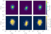 |
Fig. 1 Example of the six density maps for a random simulated neutron star population, which we fed into the SBI pipeline. The top and the bottom row show the P-Ṗ diagrams and the P-Ṗ averaged flux maps for each of the three surveys, respectively. In the top row, the colour represents the density in neutron star number within each bin, while in the bottom row the colour represents the averaged flux in Jy within each bin. For bins without any stars in the bottom row, the average flux has been set to −7. |
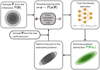 |
Fig. 2 Schematic representation of the workflow for the TSNPE algorithm applied to pulsar population synthesis. |
3.2 Truncated sequential neural posterior estimator
In Paper I, we showed how an amortized neural posterior estimator effectively constrains the initial period and magnetic field at birth for the isolated Galactic neutron stars population. However, the number of parameters that we could infer (the five magneto- rotational parameters) was limited due to the high computational cost of producing simulations across the entire parameter space. In this work, we increase the number of inferred parameters to seven by adapting the luminosity law of the Galactic pulsar population (see Equation (7)). To achieve this, we employ TSNPE (Deistler et al. 2022). This approach is significantly more simulation-efficient, as it directs the simulation effort toward the regions of the parameter space that align with the observations. This method is very promising for complex astrophysical simulators and has, for example, been successfully used to perform parameter inference for ringdown gravitational waves (Pacilio et al. 2024) and estimate distances of dwarf galaxies (Miller et al. 2021). We summarise the workflow of this algorithm in Figure 2. The TSNPE technique uses the following steps:
Sample the proposal prior distribution to obtain θi ~ P(θ).
Using the simulator, generate synthetic data xi ~ P(x|θi) based on θi from step 1.
Train the neural density estimator on the dataset composed of pairs (θi , xi) obtained in the previous steps.
Use the trained neural density estimator to approximate the posterior distribution P(θ| x0) at the observed data, x0 .
Restrict the prior distribution to the approximated posterior distribution computed in step 4 (see Section 3.3 below).
Update the proposal prior distribution with the new restricted prior and return to step 1.
We refer to each iteration of this process as ‘round’ and the process continues until the posterior distribution converges. Initially, the proposal prior covers the entire parameter space. However, as the first-round posterior is used to refine the prior in the subsequent round, we do not need to sample as broadly as in NPE. The first round provides a rough approximation of the posterior, which removes regions of the parameter space that do not align with the observed data, allowing the subsequent rounds to focus on the more relevant areas. This efficient exploration reduces the total training dataset size significantly. Furthermore, in each round, we train the neural network using the simulations generated from previous rounds combined with those generated in the current round.
3.3 Restricted prior distribution
We denote the restricted prior as P(θ)Pθ∈ℳ, where ℳ is the support of the approximated posterior at the observed data, i.e.  , and P is the indicator function. This means that for all θ ∈ ℳ the restricted prior is equal to the prior while it is 0 otherwise (see Figure 2). We note that the support, ℳ, refers to the region of the parameter space where the posterior distribution has non-negligible probability mass, essentially indicating the plausible values for the parameters given the observed data. In the following, we restrict the prior to be proportional to the highest-density region of the approximated posterior distribution, which defines the smallest region of the distribution that includes 1 − ϵ of the total probability mass. The value of ϵ is a model hyperparameter, which we fix to ϵ = 10−4 for simplicity, meaning that only 0.01% of the posterior distribution’s support is excluded. To sample the restricted prior distribution and generate parameter samples for the next round, two methods can be used: the rejection method and the Sampling importance resampling (SIR) algorithm (Rubin 1987).
In the rejection method, samples are drawn from the prior and accepted if and only if their probability under the approximate posterior is above a certain threshold. However, this approach can lead to a high rejection rate, resulting in unfeasible computation times. In contrast, the SIR algorithm avoids this issue by taking advantage of the relationship
 (17)
(17)
and the fact that the approximated posterior distribution qF(x0,ϕ) (θ) is easy to sample. The SIR algorithm draws K samples {θ1, …, θk} from the approximated posterior distribution and computes their respective weights  . These K samples are then resampled according to the distribution of the normalised weights,
  , to obtain
  with m ∈ {1, . . . , M}. It can be shown that the cumulative distribution of the normalised weights is equivalent to the cumulative distribution of the restricted prior (see Section 3.2 of Smith & Gelfand 1992). Therefore, these new samples
  follow the restricted prior distribution P(θ) P θ ∈ ℳ when K → ∞. K is a hyperparameter of the algorithm. In this work, we follow the suggestion by Deistler et al. (2022) and set K = 1024.
3.4 Approximated posterior validation
Before evaluating the quality of our posterior approximation at each round, we first need to introduce the concept of coverage probability (Cook et al. 2006). Coverage probability measures how often the ground truth falls within the estimated credible interval (CI) of the posterior distribution for a set of test samples. For example, a 95% CI with a 99% coverage probability means that, for 99% of the test samples, the ground truth lies within the 95% CI of the approximated posterior distribution. Therefore, the coverage can be used as a metric to assess the quality of the approximated posterior distribution in our test dataset.
For a well-calibrated approximated posterior distribution, the coverage probability will match the intended credibility level, resulting in a diagonal line when plotted. A conservative model, however, will have a higher coverage probability and produce wider approximated posterior distributions that contain the true parameter more frequently, thus lying above the diagonal. A conservative estimate, hence, reduces the risk of excluding the ground truth values. In contrast, an overconfident model has a lower coverage probability, resulting in approximated posterior distributions that are too narrow and often miss the ground truth value, placing its coverage probability below the diagonal.
To assess our predictions after training, we generate a test dataset using the proposal prior from the current round, combined with the test datasets from all previous rounds. Then, we compute the coverage probability on this combined test dataset to assess the quality of the estimation. Our goal is to achieve a conservative coverage probability, ensuring a broader posterior distribution (Hermans et al. 2021). This strategy helps prevent the exclusion of regions in the parameter space that might match the observed data when restricting the prior using the approximated posterior.
3.5 Deep learning setup
In this work, our neural density estimator consists of a convolutional neural network (CNN) combined with a mixture density network (MDN), the same network structure as used in Paper I. The CNN takes the density maps described in Section 2 as input and extracts key features into a latent vector of size 32, which is then fed into the MDN. The CNN architecture includes two 2D-convolutional layers, each followed by a 2D max pooling layer. The MDN, a fully connected neural network, outputs the parameters of a Gaussian mixture that approximates the posterior distribution. It contains three fully connected layers with 32 neurons each, followed by an output layer comprising four fully connected sub-layers, corresponding to the mean, weight, diagonal, and upper triangular components of the covariance matrices for the Gaussian mixture. We set the number of components in the mixture to 10, ensuring sufficient flexibility if the posterior is far from a Gaussian distribution.
Moreover, we fix the batch size to 8 and the learning rate to 5 × 10⁻⁴ . The neural network is trained using the Adam opti- miser (Kingma & Ba 2014), and we apply an early stopping criterion of 20 epochs to prevent overfitting. This implies that training is stopped if the validation metric does not improve for 20 consecutive epochs, with the best validation weights saved. The weights for the CNN are initialized using the Kaiming prescription (He et al. 2015), while for the MDN the weights are initialised with PyTorch’s default initialisation. The neural density estimator is implemented using the open-source Python package sbi (Tejero-Cantero et al. 2020). The training process is executed on a Tesla V100 SXM2 GPU with 32 GB of memory. The generation of simulations in each TSNPE round for both the training and test datasets are parallelised to speed up the algorithm. For this, we use the Python package Dask (Dask Development Team 2016), a library for dynamic task scheduling. In total, 600 CPU workers are employed to handle the parallelised simulations. We have tested the robustness of the results presented in Section 5 to variations of these hyper-parameters with additional experiments.
4 Experiments
We perform two sets of experiments: The first set focuses on testing the TSNPE methodology with our pulsar population synthesis, while the second set applies this tested methodology to infer seven parameters (five magneto-rotational parameters and two related to the radio luminosity) for the observed neutron star population. For the testing experiments, we follow two strategies: Experiments 1 and 2 involve inferring the same five magneto-rotational parameters on the observed pulsar population as in Paper I: µlog B, σlog B, µlog P, σlog P, and alate. We use the results from Paper I as a reference for comparison. In test Experiment 3, we expand the parameter space by including two additional luminosity-related parameters,  and α, resulting in a total of seven parameters. In this case, we also add the three P-Ṗ averaged flux maps as input to our neural network. This final test involves inferring these seven parameters for a simulated population with known ground truths, θ. Once we have assessed the quality of our inference technique, we infer the parameters related to the magneto-rotational evolution and the luminosity for the observational data using the fluxes from the TPA program recorded by the MeerKAT telescope (Experiments 4 and 5). All the experiments are summarised in Table 1.
For all experiments, we first generate the training and testing datasets for the first round. Since the initial prior distribution is the same across experiments with the same number of parameters, the training and testing datasets of the first round are shared between the corresponding experiments. For Experiments 1 and 2, we reuse the simulated dataset from Paper I and extract a random subsample to match the various sizes of our training and testing datasets for the first round as outlined below. On the other hand, for experiments inferring seven parameters, we generate training and testing datasets of 10 000 and 300 simulations, respectively, using the following uniform priors:
 (18)
(18)
The prior ranges for the first five parameters match those used in Paper I, while the luminosity parameters are based on the ranges from Cieślar et al. (2020), although rescaled to match our specific luminosity law in Equation (7). For the experiments constraining five magneto-rotational parameters, we only use the three P-Ṗ maps as in Paper I as an input (shown in the top row of Figure 1). On the other hand, when inferring the parameters related to the luminosity together with those related to the magneto-rotational evolution in Experiments 3–5, we add the three P-Ṗ averaged flux maps (see bottom row of Figure 1). As a result, in this case the input for the neural network consists of six maps.
To manage the computational expenses of generating new simulations from the restricted priors in subsequent rounds, we fix the number of simulations generated in each round for the training dataset. From rounds 2 through 10, the newly generated simulations for the training dataset are fixed at 1000 simulations, and for the test dataset at 300 simulations. This setup provides sufficient data to train the model and evaluate the coverage probability in each round while maintaining manageable computational costs. In each round, l0% of the training dataset is used for validation.
All experiments are run for 10 rounds allowing us to track how the posterior distributions evolve across the rounds. Additionally, we train the neural networks from scratch in each round, i.e., the weights are randomly initialized at the start of every round. We opt for this approach because we observe that using pre-trained weights from previous rounds tends to result in overconfident posterior approximations. For each round, we train five independent neural networks with identical hyperparameters and architecture on the same training dataset. The only difference between them is the randomly initialized weights. The predictions from these five networks are then combined to form an ensemble posterior distribution (see Section 4.2 of Paper I, for details on the ensemble). We adopt this approach because, when using a single neural network, the coverage probability suggests the posterior distribution to be overconfident, i.e., the approximated posterior is narrower than the true distribution (see Section 3.4 for details on coverage probability). By using an ensemble, we avoid restricting the prior distribution too much, thus preventing the exclusion of relevant regions in the parameter space (Hermans et al. 2019).
Summary of the experiments performed in this study.
5 Results
5.1 Five-parameter test: Magneto-rotational
We first assess the performance of the TSNPE algorithm (explained in Section 3.2) when inferring the same number of parameters as in Paper I to test its performance. We use the results of Paper I as a benchmark for this five-parameter experiments. Figures A.1 and A.2 in Appendix A show the results of the Experiments 1 and 2, respectively. Each row displays the 1D marginal posterior distribution for each parameter for a given round, with the coverage probability shown in the last column. We note that the x-axis range in each of the 1D marginal posterior distributions is the initial prior range.
In Experiment 1, where we use 1000 simulations for the first round, the approximated posterior distributions (shown in blue in Figure A.1) for the period parameters (µlog P, σlog P) are broad. The posterior support spans a range that is similar to the prior distribution. In contrast, for the magnetic field parameters (µlog B, σlog B, alate), the first round already narrows down a significant portion of the parameter space allowing subsequent rounds to achieve better approximations and tighter posterior distributions. While the approximated posterior distribution for the initial magnetic field quickly converges after round 2, the inferred posterior for the initial period and magnetic field decay at late times does not appear to converge to a fixed distribution. Instead, the distributions for these parameters shift slightly from one round to the next and no longer seem to narrow further after round 8. Additionally, examining the coverage probability, we see that it closely follows slightly above the diagonal, indicating a conservative estimate of the posterior distribution for all rounds that does not improve significantly as the TSNPE progresses. We associate this with the fact that the test dataset in each round includes simulations generated in that round, along with those from previous rounds. The inferred posterior distributions for the magnetic field at birth agree with those approximated in Paper I (shown in black). This is not the case for the approximated posteriors for the initial period and magnetic field decay at late times as they are shifted compared to the estimates of Paper I. We however note that these posteriors are also approximations obtained using Neural posterior estimation (NPE) and should not be taken as the ground truth.
Given these observed shifts in some of the parameters, we also test the effect of increasing the training dataset size in the first round to 10 000 simulations in Experiment 2. The corresponding results are shown in Figure A.2. In the first round, the posterior distributions for all parameters are already well constrained. While in this initial round the approximated posteriors for the initial magnetic field align with those of Paper I, the initial period approximated posteriors still show slight shifts compared to our earlier results. However, as the rounds progress, the inferred posterior gradually aligns more closely with the results from Paper I. Additionally, by round 7, the parameter alate begins to exhibit bimodality, similar to what was observed in our previous study. This bimodality arises because the individual neural networks within the ensemble produce different estimates for this parameter, as already pointed out in Section 5.5 of Paper I. We also observe some oscillations in the σlog P and alate approximated posteriors between a narrower distribution and one that aligns more closely with that of Paper I. Despite these variations, after five rounds, the posterior distributions largely agree with the estimates from Paper I. Moreover, the coverage probability moves closer to the diagonal as the rounds progress, indicating that the posterior is becoming more accurate. This demonstrates that TSNPE requires only about 19 000 training simulations to obtain well constrained posterior distributions, compared to the 360 000 simulations used in Paper I, highlighting the efficiency of TSNPE over NPE for this problem.
5.2 Seven-parameter test: Magneto-rotational and luminosity
We next apply the TSNPE method to estimate a set of seven parameters: the same five magneto-rotational parameters used in Paper I along with two additional parameters related to the bolometric intrinsic radio luminosity law of Equation (7). As a further test of our method, we first performed Experiment 3 to evaluate the quality of the approximated posterior distribution. In this experiment, the TSNPE algorithm is focused on inferring the posterior distribution of a simulated population of neutron stars with known ground truth parameters θ.
The results of Experiment 3 are presented in Figure A.3 in Appendix A. Similar to previous experiments, each row depicts the 1D marginal posterior distribution for each parameter, with the last column showing the coverage probability for the test dataset. In Figure A.3, we mark the ground truth parameters, θ, by orange dashed lines.
During the first round the posterior approximations for the initial period parameters (µlog P , σlog P) and the magnetic field decay at late times parameter (alate ) remain as broad as the prior ranges. For the parameters related to the initial magnetic field distribution (µlog B, σlog B) and the luminosity law ( , α), the algorithm already discards significant portions of the parameter space in this first round, enabling more refined approximations in subsequent rounds. We highlight that the true value is not necessarily expected to coincide with the peak of the posterior distribution. By definition, a well-calibrated posterior distribution should have coverage that aligns with the diagonal, meaning that, for instance, 99% of the ground truth values will fall within the 99% CI of the respective approximated posteriors. Therefore, while the ground truth may not match the peak of the posterior, it should lie within the support of the approximated posterior. In Figure A.3, the ground truth falls within the 95% CI (shaded in gray), demonstrating that TSNPE successfully recovers the posterior distribution for the simulated neutron star population when using a total of 1000 simulations.
We further observe that as the rounds progress, the coverage stays above the diagonal, suggesting that the posterior estimates are slightly conservative, without significant changes as we iterate through the TSNPE algorithm. For the σlog B parameter, an interesting phenomenon occurs in the early rounds. While in the first round, the approximated posterior distribution is shifted relative to the ground truth, in the second round, a secondary peak forms close to this value. By the third round, the neural network appears to favor this secondary peak, which aligns with the ground truth. In subsequent rounds, the approximated posterior converges to the posterior from this round, highlighting the efficiency of the algorithm.
5.3 Magneto-rotational and luminosity estimation inferred from the observed population
As we have demonstrated the effectiveness of TSNPE when applied to our pulsar population synthesis, we now turn our attention to the main results of this work where we infer the parameters related to the luminosity and the magneto-rotational evolution for the observed population in Experiments 4 and 5. The difference between these experiments is the number of simulations in the first round (see Table 1). As we observe no significant differences in the inference results between them, we only present the results of Experiment 4 in Figure 3. The consistency between both experiments increases our confidence in the robustness of the inference results.
In the first round of Experiment 4, as in Experiment 3, the 1D marginals of the approximated posterior distribution for the parameters µlog P , σlog P and alate remain as broad as the prior ranges. However, for µlog B, σlog B,  and α, a wide range of the parameter space is removed, which helps better constrain the initial period distribution and the late-time magnetic field decay in subsequent rounds.
For all the parameters with the exception of µlog P and σlog P , the approximated marginal posterior distributions converge after round 5. On the other hand, for the initial period parameters, we observe a small shift in the left tail of the marginal posteriors from one round to the next, beginning in round 7. Although the shift is small, we conservatively use the results from round 6 as the best estimate. At this point, the marginal posterior distribution is sufficiently broad to cover the range of values observed in rounds 7–10. A corner plot for the 1D and 2D posteriors of round 6 is illustrated in Figure 4. Corresponding medians are shown in light blue. In the 2D marginal posterior distribution, we observe correlations between several parameters. For this reason, we compute the Pearson and Spearman correlation coefficients and consider parameters to be correlated if and only if their absolute value is greater than 0.5 and the corresponding p-value < 0.05. As a result, we observed strong correlations between the parameters related to the luminosity and the initial period as well as the magnetic field distributions. We discuss the physical interpretations of these correlations in detail below.
In contrast to our results in Paper I and Experiments 1 and 2, the alate parameter appears to be well constrained and does not exhibit any bimodality or shifts between rounds. We will further discuss our interpretation of this improvement in the next section. Finally, in the rightmost panels of Figure 3, we observe the coverage probability to remain above the diagonal for all rounds without significant changes between them, indicating a conservative estimate of the approximated posterior distribution.
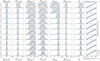 |
Fig. 3 Illustration of the TSNPE algorithm applied to our pulsar population synthesis. Here, we show the results for inferring the seven free parameters related to the magneto-rotational evolution and the luminosity for the observed neutron star population, using 1000 simulations in the first round in Experiment 4. Each row corresponds to one round of inference. The last column shows the coverage probability computed on the test dataset. In each panel, the current round’s computed values are shown in blue, while values from previous rounds are shown in light grey. The grey shaded area in the one-dimensional marginal posterior represents the 95% credibility interval of the approximated posterior for that round. In each of these 1D marginal posterior distributions, the horizontal axes represent the parameters’ prior ranges. The results from Experiment 5 are qualitatively similar to those presented here. |
6 Discussion
6.1 Inference technique: TSNPE
We begin our discussion by comparing the results of this work based on TSNPE with those obtained in Paper I using NPE. While for the initial magnetic field the estimated distributions match the estimates of Paper I, the new inferred distributions for the initial period and magnetic field decay at late times differ slightly from these previous estimates. These differences are more pronounced when we use 1000 simulations in the first round (see Figure A.1). However, when the first round training dataset size is increased to 10 000 simulations, the approximated posteriors move closer to the previous estimates, and by round 10, they closely align with those in Paper I (See Figure A.2). This behaviour is expected as the network is trained with more simulations and thus gains better insight into the parameter landscape, allowing the network to more accurately approximate the posterior distribution. However, when inferring seven parameters for the observed population, the results obtained by round 10 using 10 000 simulations for the training in the first round are comparable to those obtained with only 1000 initial training simulations. This suggests that the 1000 training simulations used in the first round are already sufficient for the neural network to estimate the seven parameters, and adding more does not provide additional information for this task. As discussed below in detail, we associate this improvement with the addition of flux measurements as inputs to the neural density estimator.
The broader marginal posterior distributions for the initial period, compared to the narrower constraints on the other parameters, suggest a degeneracy in the initial period. For example, in Figure 3 where we infer the seven parameters for the observed data, the distribution for the initial magnetic field in the first round is already very narrow. In contrast, the distribution for the initial period remains relatively broad even in the final round, showing a slight shift across rounds. This suggests that estimating µlog P and σlog P is a challenge, as already noted in earlier works using different inference methods (Gullón et al. 2014; Graber et al. 2024). As previously discussed in Section 5.3 of Paper I, the initial period information is gradually lost during the evolution of neutron stars in the P-Ṗ diagram. This effect is easily visualized when the magnetic field is constant, although similar reasoning applies when decay is introduced: Two neutron stars with different initial periods but the same initial magnetic field at birth lie on the same constant magnetic field line in the P-Ṗ diagram. Although both sources move along this constant field line throughout their evolution, the one with a shorter period evolves faster than the one with a longer period (see Equation (4)). Therefore, by the end of the simulation, both sources end up in similar locations in the P-Ṗ plane, making it difficult to distinguish between them. This degeneracy effectively leads to broad posterior distributions for the initial period as observed.
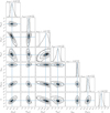 |
Fig. 4 Inference results for the observed pulsar population using round 6 of Experiment 4. The corner plot shows 1D and 2D marginal posterior distributions for the five magneto-rotational parameters and the two parameters related to the intrinsic bolometric luminosity. We highlight the medians in light blue. Corresponding values and 95% CIs are summarized above the panels and in Equation (19). |
6.2 Magnetic field decay at late times
Now we turn our attention to the magnetic field decay at late times. When we infer seven parameters and add the flux measurement as input, this parameter is narrowly constrained, indicating that the density estimator is confident in the inference of this parameter. This is evident in the fifth panel of Figure 3. This is in contrast to what we observe in Paper I and in the testing experiments where we infer five parameters, which estimate a broader and bimodal distribution. Bimodality in the posterior distribution for this parameter arises when the different neural networks in the ensemble disagree, leading to non-overlapping supports.
To investigate the reason for the improved alate constraints, we focus on the two main changes in this work beyond the TSNPE implementation: (i) modifying our luminosity prescription (see Equation (7)) and adding two additional free parameters and (ii) providing additional P-Ṗ averaged flux maps. The former is relevant because the bolometric intrinsic luminosity is proportional to the loss of the rotational energy and the dipolar magnetic field and luminosity are thus related. Therefore, the luminosity of old neutron stars (i.e., tage > τlate) is influenced by the alate value. This effect should primarily affect the synthetic SMPS populations which focus on high latitudes and contain a larger fraction of old pulsars with respect to young pulsars compared to PMPS and HTRU. Specifically, for two simulations with identical parameters but different alate values, the P-Ṗ averaged flux maps for SMPS can differ significantly while PMPS and HTRU are unaffected. We explore this effect on our inference by computing the correlation between alate and those parameters related to the luminosity in the 2D posteriors in Figure 4. We find that both the Pearson and Spearman coefficients are lower than 0.5, indicating no significant correlation between these two variables. We emphasise, however, that the influence of alate is primarily on the SMPS, while the correlation is computed across all three surveys. The coefficients are thus not overly sensitive to this correlation. Additionally, we note that the luminosity prescription used when constraining seven parameters differs slightly from that applied when inferring only five, where the prescription from Paper I was applied. Nonetheless, we cannot associate the new luminosity prescription solely with the improved alate constraints presented in this work.
Therefore, we now turn our attention to the effect of adding the P-Ṗ averaged flux maps as input to the neural density estimator. To test this, we perform an experiment where we infer the seven parameters providing only the three P-Ṗ density maps. We observe that the alate posterior becomes broader, and bimodality arises, highlighting the importance of the flux measurements in the inference process. Additionally, this experiment shows that the approximated posterior distributions for parameters related to the initial period and luminosity become broader as well. Providing the density estimator with additional information on the fluxes of the pulsar population when inferring the magnetic field at late times turns out to be crucial and enhances the overall inference accuracy.
6.3 Best estimated parameters with TSNPE
After assessing the quality of the TSNPE algorithm with the testing experiments, we used this technique to infer the magneto- rotational luminosity parameters for the observed population. In particular, we chose as our ‘best estimates’ the values from round 6 of Experiment 4 as outlined above in Section 5.3. Using the corresponding density estimator, we find the following best estimates at 95% credible level:
 (19)
(19)
From the Pearson and Spearman correlation coefficients calculated for the 2D marginals shown in Figure 4, we find a positive correlation between  and
and  , which indicates that higher initial magnetic fields require an increase in
  to fit the observed data. This relationship is expected because a higher B0 shifts the Ṗ distribution of detected pulsars towards higher values. To match the observations, the model requires an increase in luminosity facilitating the detection of pulsars with lower Ṗ. We also observe a negative correlation between
  and
and  . Therefore, a longer initial period distribution leads to a lower
  . Increasing
  shifts the simulated population to the right in the P-Ṗ diagram since pulsars with lower rotational energy become detectable. This shift requires the population to move toward shorter final periods to align the simulated population with observations. This, in turn, can be compensated by a shift towards shorter periods, resulting in the observed anti-correlation.
Finally, we compared the simulated population using the best-estimated parameters shown in Equation (19) and the observed population. Although an exhaustive comparison is beyond the scope of this work, we run a simulation with these best estimates and provide Figures 5 and 6 to discuss the main aspects. In Figure 5, we show the P-Ṗ maps for both the observed and the simulated neutron star populations for each of the surveys. The simulated pulsar population closely resembles the observed population. Notably, in Paper I, the SMPS sample showed a slight shift towards lower Ṗ values, which we attributed to the weak constraints on alate parameter. We do not observe the same shift in this work as we more tightly constrain this value with the TSNPE algorithm. Overall, the distributions of the best-estimated simulated neutron star population closely resemble those of the observed population, giving us confidence in our inference results. Moreover, in Figure 6, we show the kernel density estimation (KDE) fits for the flux density distribution obtained with a Gaussian kernel, to easily compare between the observed and simulated populations. While the distributions for both PMPS and HTRU closely follow those of the observed population, the simulated fluxes for SMPS differ slightly from the observed ones. This discrepancy might hint at missing physics at late times because (as we already mentioned) SMPS is more sensitive to old pulsars compared to the other two surveys.
To compute the inferred birth rate for each survey, we run 10 different simulations using the best-parameter estimates. The resulting means and standard deviation for the birthrates are as follows:
 (20)
(20)
These estimates are comparable to those found in Paper I and compatible with the recent core-collapse supernova rate inferred by Rozwadowska et al. (2021).
Finally, Table 2 compares the results of this work with previous studies. The inferred initial magnetic field distribution is consistent with prior estimates that apply a similarly realistic prescription for the magnetic field decay, as in the work of Gullón et al. (2014) and in Paper I. However, the initial period distribution tends toward slightly larger values compared to Paper I and previous works. In the former, this difference may be explained by the fact that we fix the value of  to a higher value in Paper I than estimated here. The anti-correlation between
  and
and  , therefore, biases the inference of the initial period distribution toward shorter periods. On the other hand, Igoshev et al. (2022) analysed 56 young neutron stars associated with supernova remnants and studied their magneto-rotational properties only. Their estimates may be biased due to the small number of relatively young sources in their analysis, which could explain the discrepancy between their work and this one. We further note that our results cannot be directly compared with those of Sautron et al. (2024) as their study does not include parameter estimation and adopts a pseudo-luminosity prescription instead of the intrinsic bolometric luminosity used here. On the other hand, the relationship we found between the luminosity, P, and Ṗ is consistent, within uncertainties, with the results of Shi & Ng (2024). However, their inferred normalisation factor, L0 , differs considerably from ours, likely due to a completely different beaming prescription. Additionally, both Sautron et al. (2024) and Shi & Ng (2024) employ magnetic field decay prescriptions that differ significantly from the one used in this work, which additionally contributes to the observed discrepancies in the inferred parameters.
7 Summary
In this work, we demonstrate how combining a sequential SBI approach with a pulsar population synthesis framework together with consistent flux measurement allows us to successfully infer the parameters related to magneto-rotational evolution. This new approach also sheds light on the distribution of the intrinsic bolometric radio luminosity of the Galactic isolated neutron star population. Our main findings are as follows:
When inferring the parameters related to the luminosity and the magneto-rotational evolution, we include flux measurements as an additional input. Specifically, for the observed neutron star population, we use data from the TPA program recorded by the MeerKAT telescope, as reported by Posselt et al. (2023). This dataset is the largest unified neutron star catalogue with consistent flux measurement. Incorporating flux information not only helps us constrain the luminosity but also leads to tighter constraints on the late-time magnetic field decay, compared to our previous work.
We successfully recover narrow posterior distributions for the parameters related to the magnetic field and the luminosity. The inferred period distribution is broader compared to the rest of the parameters. This is expected due to the degeneracies between the period and already noted in previous works using different inference techniques. Overall, the approximated posterior distributions obtained are consistent with previous studies.
While our previous study using NPE (see Paper I) required 360 000 training simulations to estimate the five magneto- rotational parameters, here we achieve comparable results with only 19 000 simulations due to the efficiency of the sequential technique (see Figure A.2). This efficiency enables us to expand the number of inferrable parameters which was unfeasible with the NPE method.
As mentioned previously and also noted in Paper I and other works, the posterior distribution for the initial period is difficult to constrain, resulting in a broader distribution. This is because the information about the initial period is lost during evolution, making it challenging for any inference approach to estimate these parameters. New pulsar surveys in the radio band, as well as in other wavelengths, will increase the number of observed neutron stars, which may help constrain the neutron star population further. Moreover, it is crucial to include the entire pulsar population, not just radio pulsars. As shown in Gullón et al. (2015), including magnetars, highly magnetized neutron stars emitting X-rays, help constrain the higher end of the magnetic field distribution at birth. Current population synthesis models are naturally biased toward lower magnetic field neutron stars.
Furthermore, as reflected in the discrepancies between the simulated flux distribution for the SMPS survey and the observed data, we are still missing some relevant physics in the latetime evolution. Comparing different prescriptions for magnetic field decay at late times, will be crucial in the future. Having demonstrated that TSNPE can successfully infer multiple parameters of the isolated pulsar population synthesis with a reduced simulation budget. Model comparison with SBI as e.g. introduced in Spurio Mancini et al. (2023) is now within reach to help us deepen our understanding of the evolution of old pulsars further.
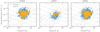 |
Fig. 5 Simulated and observed populations of isolated Galactic radio pulsars. Each panel corresponds to a different survey, from left to right: PMPS, SMPS, and the low- and mid-latitude HTRU survey. The yellow stars indicate the observed pulsar population with data taken from the ATNF Pulsar Catalogue (Manchester et al. 2005, v2.5.1). The blue dots represent the simulated pulsar population for the parameters inferred via TSNPE (see Equation (19)). Lines of constant spin-down power (|Ėrot|) and constant dipolar surface magnetic field are also shown. |
Comparison between best parameters for the log-normal initial magnetic-field, initial period distributions, and the magnetic field decay at late times in the literature.
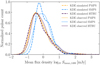 |
Fig. 6 Distributions of mean radio flux densities, Smean,1400, at 1400 MHz for the populations of isolated Galactic radio pulsars in the PMPS, the SMPS, and the low- and mid-latitude HTRU survey (in yellow, light blue and purple, respectively). We show the individual probability density functions obtained via KDE using a Gaussian kernel to facilitate comparison. Estimates for the observed population are shown as solid lines, while our best-parameter simulation is shown with dashed lines. Data taken from the TPA program (Posselt et al. 2023). |
Acknowledgements
The authors thank Emilie Parent for useful exchanges on radio pulsar emission and detections, Clara Dehman for providing magnetic field evolution curves, Bettina Posselt and Aris Karastergiou for useful discussion and insights on the TPA program data, and Michael Deistler and Maximilian Dax for valuable discussions on SBI and TSNPE. The data production, processing, and analysis tools for this paper have been implemented and operated at the Port d’Informació Científica (PIC) data center. PIC is maintained through a collaboration of the Institut de Física d’Altes Energies (IFAE) and the Centro de Investigaciones Energéticas, Medioambientales y Tecnológicas (Ciemat). We particularly thank Christian Neissner and Martin Børstad Eriksen for their support at PIC. C.P.A., M.R. and N.R. are supported by the ERC via the Consolidator grant “MAGNESIA” (No. 817661), the ERC Proof of Concept "DeepSpacePULSE" (No. 101189496), and by the program Unidad de Excelen- cia María de Maeztu CEX2020-001058-M. V.G. is supported by a UKRI Future Leaders Fellowship (grant number MR/Y018257/1). We also acknowledge support from the Catalan grant SGR2021-01269 (PI: Graber/Rea) and the Spanish grant ID2023-153099NA-I00 (PI: Coti Zelati). C.P.A.’s work has been carried out within the framework of the doctoral program in Physics at the Universitat Autonoma de Barcelona.
Appendix A Test experiments
Figures A.1 to A.3 display the results of the TSNPE algorithm over 10 rounds for Experiments 1 to 3, discussed in Sections 5.1 and 5.2. These experiments focus on testing the TSNPE methodology with our pulsar population synthesis. In Experiments 1 and 2, we focus on inferring the five magneto-rotational parameters and compare the results with those obtained in Paper I. In Experiment 3, we infer the five magneto-rotational parameters along with those related to the intrinsic radio luminosity distribution for a simulated neutron star population with known ground truth, θ.
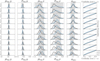 |
Fig. A.1 Illustration of the TSNPE algorithm applied to our pulsar population synthesis. Here, we show results for inferring the five magneto- rotational parameters (as for Paper I) of the observed neutron star population in Experiment 1 with 1000 simulations in round 1. Each row corresponds to one round of inference. The last column shows the coverage probability computed on the test dataset. In each panel, the current round’s computed values are shown in blue, while values from previous rounds are shown in light grey. The grey shaded area in the one-dimensional marginal posterior represents the 95% credibility interval of the approximated posterior for that round. In each of these 1D marginal posterior distributions, the horizontal axes represent the parameters’ prior ranges. For comparison, the posterior distribution estimated in Paper I is shown as black solid lines. |
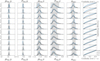 |
Fig. A.2 Same as Figure A.1 but for Experiment 2, where we increased the size of the initial training dataset to 10 000 simulations. |
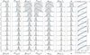 |
Fig. A.3 Similar to Figure A.1 but for Experiment 3, where we applied the TSNPE algorithm to infer both the magneto-rotational parameters and the parameters related to the intrinsic bolometric luminosity from Equation (7). This inference was performed for a simulated neutron star population, and the ground truth values, θ, are represented by the orange dashed lines. |
References
- Alsing, J., Charnock, T., Feeney, S., & Wandelt, B. 2019, MNRAS, 488, 4440 [Google Scholar]
- Barret, D., & Dupourqué, S. 2024, A&A, 686, A133 [NASA ADS] [CrossRef] [EDP Sciences] [Google Scholar]
- Bates, S. D., Lorimer, D. R., Rane, A., & Swiggum, J. 2014, MNRAS, 439, 2893 [NASA ADS] [CrossRef] [Google Scholar]
- Bhardwaj, U., Alvey, J., Miller, B. K., Nissanke, S., & Weniger, C. 2023, Phys. Rev. D, 108, 042004 [Google Scholar]
- Chen, K., & Ruderman, M. 1993, ApJ, 402, 264 [NASA ADS] [CrossRef] [Google Scholar]
- Cieślar, M., Bulik, T., & Osłowski, S. 2020, MNRAS, 492, 4043 [Google Scholar]
- Coleman, M. S. B., & Burrows, A. 2022, MNRAS, 517, 3938 [NASA ADS] [CrossRef] [Google Scholar]
- Cook, S., Gelman, A., & Rubin, D. 2006, J. Comput. Graph. Stat., 15, 675 [CrossRef] [Google Scholar]
- Cranmer, K., Brehmer, J., & Louppe, G. 2020, Proc. Natl. Acad. Sci., 117, 30055 [Google Scholar]
- Dai, S., Johnston, S., & Hobbs, G. 2017, MNRAS, 472, 1458 [NASA ADS] [CrossRef] [Google Scholar]
- Dask Development Team 2016, Dask: Library for dynamic task scheduling [Google Scholar]
- Dax, M., Green, S. R., Gair, J., et al. 2021, Phys. Rev. Lett., 127, 241103 [NASA ADS] [CrossRef] [Google Scholar]
- Deistler, M., Goncalves, P. J., & Macke, J. H. 2022, in Advances in Neural Information Processing Systems, eds. S. Koyejo, S. Mohamed, A. Agarwal, et al. (UK: Curran Associates, Inc.), 35, 23135 [Google Scholar]
- Edwards, R. T., Bailes, M., Van Straten, W., & Britton, M. C. 2001, MNRAS, 326, 358 [NASA ADS] [CrossRef] [Google Scholar]
- Faucher-Giguère, C.-A. & Kaspi, V. M. 2006, ApJ, 643, 332 [CrossRef] [Google Scholar]
- Goldreich, P., & Julian, W. H. 1969, ApJ, 157, 869 [Google Scholar]
- Gonthier, P. L., Story, S. A., Clow, B. D., & Harding, A. K. 2007, Ap&SS, 309, 245 [NASA ADS] [CrossRef] [Google Scholar]
- Graber, V., Ronchi, M., Pardo-Araujo, C., & Rea, N. 2024, ApJ, 968, 16 [CrossRef] [Google Scholar]
- Greenberg, D. S., Nonnenmacher, M., & Macke, J. H. 2019, arXiv e-prints [arXiv:1905.07488] [Google Scholar]
- Gullón, M., Miralles, J. A., Viganò, D., & Pons, J. A. 2014, MNRAS, 443, 1891 [CrossRef] [Google Scholar]
- Gullón, M., Pons, J. A., Miralles, J. A., et al. 2015, MNRAS, 454, 615 [CrossRef] [Google Scholar]
- He, K., Zhang, X., Ren, S., & Sun, J. 2015, arXiv e-prints [arXiv:1502.01852] [Google Scholar]
- Hermans, J., Begy, V., & Louppe, G. 2019, arXiv e-prints [arXiv:1903.04057] [Google Scholar]
- Hermans, J., Delaunoy, A., Rozet, F., et al. 2021, arXiv e-prints [arXiv:2110.06581] [Google Scholar]
- Hobbs, G., Lorimer, D. R., Lyne, A. G., & Kramer, M. 2005, MNRAS, 360, 974 [Google Scholar]
- Igoshev, A. P. 2020, MNRAS, 494, 3663 [NASA ADS] [CrossRef] [Google Scholar]
- Igoshev, A. P., Frantsuzova, A., Gourgouliatos, K. N., et al. 2022, MNRAS, 514, 4606 [CrossRef] [Google Scholar]
- Jacoby, B. A., Bailes, M., Ord, S. M., Edwards, R. T., & Kulkarni, S. R. 2009, ApJ, 699, 2009 [NASA ADS] [CrossRef] [Google Scholar]
- Janka, H.-T., Wongwathanarat, A., & Kramer, M. 2022, ApJ, 926, 9 [NASA ADS] [CrossRef] [Google Scholar]
- Jankowski, F., van Straten, W., Keane, E. F., et al. 2018, MNRAS, 473, 4436 [Google Scholar]
- Johnston, S., Karastergiou, A., Keith, M. J., et al. 2020, MNRAS, 493, 3608 [NASA ADS] [CrossRef] [Google Scholar]
- Keith, M. J., Jameson, A., van Straten, W., et al. 2010, MNRAS, 409, 619 [Google Scholar]
- Kingma, D. P., & Ba, J. 2014, arXiv e-prints [arXiv:1412.6980] [Google Scholar]
- Lorimer, D. R. 2004, IAU Symp., 218, 105 [NASA ADS] [Google Scholar]
- Lorimer, D. R., & Kramer, M. 2012, Handbook of Pulsar Astronomy (Cambridge: Cambridge University Press) [Google Scholar]
- Lorimer, D. R., Bailes, M., Dewey, R. J., & Harrison, P. A. 1993, MNRAS, 263, 403 [Google Scholar]
- Lorimer, D. R., Faulkner, A. J., Lyne, A. G., et al. 2006, MNRAS, 372, 777 [NASA ADS] [CrossRef] [Google Scholar]
- Lueckmann, J.-M., Goncalves, P. J., Bassetto, G., et al. 2017, arXiv e-prints [arXiv:1711.01861] [Google Scholar]
- Manchester, R. N., Lyne, A. G., Camilo, F., et al. 2001, MNRAS, 328, 17 [NASA ADS] [CrossRef] [Google Scholar]
- Manchester, R. N., Hobbs, G. B., Teoh, A., & Hobbs, M. 2005, AJ, 129, 1993 [Google Scholar]
- Miller, B., Cole, A., Forré, P., Louppe, G., & Weniger, C. 2021, Adv. Neural Inform. Process. Sys., 34, 129 [Google Scholar]
- Mishra-Sharma, S., & Cranmer, K. 2022, Phys. Rev. D, 105, 063017 [NASA ADS] [CrossRef] [Google Scholar]
- Narayan, R., & Ostriker, J. P. 1990, ApJ, 352, 222 [NASA ADS] [CrossRef] [Google Scholar]
- Pacilio, C., Bhagwat, S., & Cotesta, R. 2024, Phys. Rev. D, 110, 083010 [Google Scholar]
- Papamakarios, G., & Murray, I. 2016, arXiv e-prints [arXiv:1605.06376] [Google Scholar]
- Papamakarios, G., Sterratt, D. C., & Murray, I. 2018, arXiv e-prints [arXiv:1805.07226] [Google Scholar]
- Philippov, A., Tchekhovskoy, A., & Li, J. G. 2014, MNRAS, 441, 1879 [NASA ADS] [CrossRef] [Google Scholar]
- Popov, S. B., Pons, J. A., Miralles, J. A., Boldin, P. A., & Posselt, B. 2010, MNRAS, 401, 2675 [NASA ADS] [CrossRef] [Google Scholar]
- Posselt, B., Karastergiou, A., Johnston, S., et al. 2023, MNRAS, 520, 4582 [NASA ADS] [CrossRef] [Google Scholar]
- Rozwadowska, K., Vissani, F., & Cappellaro, E. 2021, New Astron., 83, 101498 [NASA ADS] [CrossRef] [Google Scholar]
- Rubin, D. 1987, Bayesian Stat., 3 [Google Scholar]
- Ruderman, M. A., & Sutherland, P. G. 1975, ApJ, 196, 51 [Google Scholar]
- Russ, J. C. 2011, The Image Processing Handbook, 6th edn. (USA: CRC Press, Inc.) [Google Scholar]
- Sautron, M., Pétri, J., Mitra, D., & Dirson, L. 2024, A&A, 691, A349 [NASA ADS] [CrossRef] [EDP Sciences] [Google Scholar]
- Saxena, A., Meerburg, P. D., Weniger, C., de Lera Acedo, E., & Handley, W. 2024, RAS Techniques and Instruments, 3, 724 [Google Scholar]
- Sengar, R., Bailes, M., Balakrishnan, V., et al. 2023, MNRAS, 522, 1071 [NASA ADS] [CrossRef] [Google Scholar]
- Shi, Z., & Ng, C. Y. 2024, ApJ, 972, 78 [NASA ADS] [CrossRef] [Google Scholar]
- Smith, A. F. M., & Gelfand, A. E. 1992, Am. Stat., 46, 84 [Google Scholar]
- Song, X., Weltevrede, P., Szary, A., et al. 2023, MNRAS, 520, 4562 [NASA ADS] [CrossRef] [Google Scholar]
- Spitkovsky, A. 2006, ApJ, 648, L51 [Google Scholar]
- Spurio Mancini, A., Docherty, M. M., Price, M. A., & McEwen, J. D. 2023, RAS Tech. Instrum., 2, 710 [Google Scholar]
- Stuart, A., & Ord, J. K. 1994, Kendall’s Advanced Theory of Statistics, Distribution theory (Hoboken: John Wiley & Sons Inc) [Google Scholar]
- Tejero-Cantero, A., Boelts, J., Deistler, M., et al. 2020, J. Open Source Softw., 5, 2505 [NASA ADS] [CrossRef] [Google Scholar]
- Vasist, M., Rozet, F., Absil, O., et al. 2023, A&A, 672, A147 [NASA ADS] [CrossRef] [EDP Sciences] [Google Scholar]
- Viganò, D., Rea, N., Pons, J. A., et al. 2013, MNRAS, 434, 123 [CrossRef] [Google Scholar]
- Viganò, D., Garcia-Garcia, A., Pons, J. A., Dehman, C., & Graber, V. 2021, Comput. Phys. Commun., 265, 108001 [CrossRef] [Google Scholar]
- Xu, K., Yang, H.-R., Mao, Y.-H., et al. 2023, ApJ, 947, 76 [NASA ADS] [CrossRef] [Google Scholar]
- Yao, J. M., Manchester, R. N., & Wang, N. 2017, ApJ, 835, 29 [NASA ADS] [CrossRef] [Google Scholar]
- Zhang, B., Harding, A. K., & Muslimov, A. G. 2000, ApJ, 531, L135 [NASA ADS] [CrossRef] [Google Scholar]
All Tables
Comparison between best parameters for the log-normal initial magnetic-field, initial period distributions, and the magnetic field decay at late times in the literature.
All Figures
|
Fig. 1 Example of the six density maps for a random simulated neutron star population, which we fed into the SBI pipeline. The top and the bottom row show the P-Ṗ diagrams and the P-Ṗ averaged flux maps for each of the three surveys, respectively. In the top row, the colour represents the density in neutron star number within each bin, while in the bottom row the colour represents the averaged flux in Jy within each bin. For bins without any stars in the bottom row, the average flux has been set to −7. |
| In the text | |
|
Fig. 2 Schematic representation of the workflow for the TSNPE algorithm applied to pulsar population synthesis. |
| In the text | |
|
Fig. 3 Illustration of the TSNPE algorithm applied to our pulsar population synthesis. Here, we show the results for inferring the seven free parameters related to the magneto-rotational evolution and the luminosity for the observed neutron star population, using 1000 simulations in the first round in Experiment 4. Each row corresponds to one round of inference. The last column shows the coverage probability computed on the test dataset. In each panel, the current round’s computed values are shown in blue, while values from previous rounds are shown in light grey. The grey shaded area in the one-dimensional marginal posterior represents the 95% credibility interval of the approximated posterior for that round. In each of these 1D marginal posterior distributions, the horizontal axes represent the parameters’ prior ranges. The results from Experiment 5 are qualitatively similar to those presented here. |
| In the text | |
|
Fig. 4 Inference results for the observed pulsar population using round 6 of Experiment 4. The corner plot shows 1D and 2D marginal posterior distributions for the five magneto-rotational parameters and the two parameters related to the intrinsic bolometric luminosity. We highlight the medians in light blue. Corresponding values and 95% CIs are summarized above the panels and in Equation (19). |
| In the text | |
|
Fig. 5 Simulated and observed populations of isolated Galactic radio pulsars. Each panel corresponds to a different survey, from left to right: PMPS, SMPS, and the low- and mid-latitude HTRU survey. The yellow stars indicate the observed pulsar population with data taken from the ATNF Pulsar Catalogue (Manchester et al. 2005, v2.5.1). The blue dots represent the simulated pulsar population for the parameters inferred via TSNPE (see Equation (19)). Lines of constant spin-down power (|Ėrot|) and constant dipolar surface magnetic field are also shown. |
| In the text | |
|
Fig. 6 Distributions of mean radio flux densities, Smean,1400, at 1400 MHz for the populations of isolated Galactic radio pulsars in the PMPS, the SMPS, and the low- and mid-latitude HTRU survey (in yellow, light blue and purple, respectively). We show the individual probability density functions obtained via KDE using a Gaussian kernel to facilitate comparison. Estimates for the observed population are shown as solid lines, while our best-parameter simulation is shown with dashed lines. Data taken from the TPA program (Posselt et al. 2023). |
| In the text | |
|
Fig. A.1 Illustration of the TSNPE algorithm applied to our pulsar population synthesis. Here, we show results for inferring the five magneto- rotational parameters (as for Paper I) of the observed neutron star population in Experiment 1 with 1000 simulations in round 1. Each row corresponds to one round of inference. The last column shows the coverage probability computed on the test dataset. In each panel, the current round’s computed values are shown in blue, while values from previous rounds are shown in light grey. The grey shaded area in the one-dimensional marginal posterior represents the 95% credibility interval of the approximated posterior for that round. In each of these 1D marginal posterior distributions, the horizontal axes represent the parameters’ prior ranges. For comparison, the posterior distribution estimated in Paper I is shown as black solid lines. |
| In the text | |
|
Fig. A.2 Same as Figure A.1 but for Experiment 2, where we increased the size of the initial training dataset to 10 000 simulations. |
| In the text | |
|
Fig. A.3 Similar to Figure A.1 but for Experiment 3, where we applied the TSNPE algorithm to infer both the magneto-rotational parameters and the parameters related to the intrinsic bolometric luminosity from Equation (7). This inference was performed for a simulated neutron star population, and the ground truth values, θ, are represented by the orange dashed lines. |
| In the text | |
Current usage metrics show cumulative count of Article Views (full-text article views including HTML views, PDF and ePub downloads, according to the available data) and Abstracts Views on Vision4Press platform.
Data correspond to usage on the plateform after 2015. The current usage metrics is available 48-96 hours after online publication and is updated daily on week days.
Initial download of the metrics may take a while.