| Issue |
A&A
Volume 667, November 2022
|
|
|---|---|---|
| Article Number | A82 | |
| Number of page(s) | 12 | |
| Section | Astrophysical processes | |
| DOI | https://doi.org/10.1051/0004-6361/202243305 | |
| Published online | 09 November 2022 | |
The Galactic population of canonical pulsars
1
Université de Strasbourg, CNRS, Observatoire astronomique de Strasbourg, UMR 7550, 67000 Strasbourg, France
e-mail: This email address is being protected from spambots. You need JavaScript enabled to view it.
2
National Centre for Radio Astrophysics, Tata Institute for Fundamental Research, Post Bag 3, Ganeshkhind, Pune 411007, India
3
Janusz Gil Institute of Astronomy, University of Zielona Góra, ul. Szafrana 2, 65-516 Zielona Góra, Poland
Received:
10
February
2022
Accepted:
13
June
2022
Abstract
Context. Current wisdom suggests that the observed population of neutron stars are manifestations of their birth scenarios and their thermal and magnetic field evolution. Neutron stars can be observed at various wavebands as pulsars, and radio pulsars represent by far the largest population of neutron stars.
Aims. In this paper, we aim to constrain the observed population of the canonical neutron star period, its magnetic field, and its spatial distribution at birth in order to understand the radio and high-energy emission processes in a pulsar magnetosphere. For this purpose we design a population synthesis method, self-consistently taking into account the secular evolution of a force-free magnetosphere and the magnetic field decay.
Methods. We generated a population of pulsars and evolved them from their birth to the present time, using the force-free approximation. We assumed a given initial distribution for the spin period, surface magnetic field, and spatial Galactic location. Radio emission properties were accounted for by the polar cap geometry, whereas the gamma-ray emission was assumed to be produced within the striped wind model.
Results. We find that a decaying magnetic field gives better agreement with observations compared to a constant magnetic field model. Starting from an initial mean magnetic field strength of B = 2.5 × 10⁸ T with a characteristic decay timescale of 4.6 × 10⁵ yr, a neutron star birth rate of 1/70 yr and a mean initial spin period of 60 ms, we find that the force-free model satisfactorily reproduces the distribution of pulsars in the P−Ṗ diagram with simulated populations of radio-loud, radio-only, and radio quiet gamma-ray pulsars similar to the observed populations.
Key words: pulsars: general / radiation mechanisms: non-thermal / methods: statistical / gamma rays: stars / radio continuum: stars
© L. Dirson et al. 2022
 Open Access article, published by EDP Sciences, under the terms of the Creative Commons Attribution License (https://creativecommons.org/licenses/by/4.0), which permits unrestricted use, distribution, and reproduction in any medium, provided the original work is properly cited.
This article is published in open access under the Subscribe-to-Open model. This email address is being protected from spambots. You need JavaScript enabled to view it. to support open access publication.
1. Introduction
Pulsars are rapidly rotating, highly magnetized neutron stars surrounded by a plasma-filled magnetosphere that emits regular pulses of radiation at their spin frequency. The term ‘pulsar’ comes from ‘pulsating radio source’ since they were first observed at radio wavelengths. Currently, the number of observed radio pulsars is roughly 30001 (Manchester et al. 2005). Subsequently, however, it was found that pulsars were also bright in X-rays, optical, and gamma-rays. In particular, the Large Area Telescope (LAT) on board the Fermi satellite has forcefully changed our understanding of gamma-ray pulsars by discovering dozens of radio-quiet gamma-ray pulsars as well as millisecond pulsars (MSPs). After more than ten years of operation, the LAT has detected over 250 pulsars (Abdo et al. 2013; Smith et al. 2019), establishing them as the dominant class of GeV sources in the Milky Way. This signified a new era for gamma-ray pulsar statistics, first started by EGRET with the detection of only seven pulsars (Thompson et al. 1995). These recent discoveries have raised fundamental questions, one of the most challenging amongst them being to find a physical consistent theory of pulsar multi-wavelength emission mechanisms. With the advancement of instrumental techniques, future surveys with greatly improved sensitivities are being envisaged. Amongst them, the Square Kilometre Array (SKA) is expected to be 50 times more sensitive, and is predicted to survey the sky 10 000 times faster than any existing imaging radio telescope array2. In this context, it is of utmost importance to be able to anticipate the discovery rate of new pulsars, since it enables us to validate our current understanding of pulsar emission mechanisms, as well as their evolution track and the factors impacting their detection.
Pulsar population synthesis (hereafter PPS) studies are powerful tools aiming to predict the detectability of pulsars. Inferring the underlying properties responsible for the observed pulsar population is an arduous task. Indeed, both the impact of the detection procedure and the inhomogeneous properties of the interstellar medium (ISM) have to be accurately estimated to account for possible observational biases.
Much of the progress in PPS has come from thorough Monte Carlo simulations that generate pulsars and test whether they fulfil the criteria for detection according to geometrical factors and sensitivity issues. It is then possible to develop and optimize a model for the underlying pulsar population, which informs us about the important intrinsic neutron star parameters and distribution, enabling predictions for future surveys. Usually, PPS studies follow two simple approaches. The first one is to take a ‘snapshot’ of the Galaxy as it appears today, where no assumptions are made regarding the prior evolution of the pulsar population. Instead, this population is generated assuming various distribution functions (typically spatial distribution, spin period P and,  - or Ṗ), which are optimized to match the observations. Inspired by earlier studies from Taylor & Manchester (1977) and Lyne et al. (1985), Lorimer et al. (2006) applied the snapshot approach to the canonical3 pulsar population to determine best-fitting probability density functions in Galactocentric radius (R), luminosity (L), height with respect to the Galactic plane (z), and the period P for the currently observed population of pulsars. Alternatively, one may consider ‘evolution’ strategies where the pulsars are evolved from birth up to the present era, starting from an initial spatial distribution, and an initial period and magnetic field distribution. A fine example of the latter genre is the comprehensive study of Faucher-Giguère & Kaspi (2006), which quite successfully reproduced the properties of the main part of the radio pulsar population using a model in which the luminosity has a power-law dependence on P and Ṗ. PPS studies can be also extended to the population of neutron stars observed in other bands, such as X-rays (see for instance Popov et al. 2010) and γ-rays. Indeed, with the broad increase in γ-ray pulsar numbers, a statistical treatment of the γ-ray population in combination with deep radio surveys of the Galactic plane is now feasible. Early works on radio-loud gamma-ray pulsar populations carried out before the Fermi era include Gonthier et al. (2002), (2004), (2007a,b). With the advent of Fermi/LAT, new studies emerged (see for instance Gonthier et al. 2018; Ravi et al. 2010; Takata et al. 2011; Watters & Romani 2011; Pierbattista et al. 2012), trying to constrain the geometry and the location of the gamma-ray emission sites. Watters & Romani (2011) showed that an initial spin period of P0 = 50 ms and a birth rate of one neutron star per 59 yr were required to reproduce the observed γ-ray population. They made the prediction that after ten years of operations, Fermi should detect ∼120 young γ-ray pulsars, of which about one half would be radio-quiet. Gonthier et al. (2004) included an exponentially decaying magnetic field with a 2.8 Myr timescale and displaying a satisfactory agreement with the P−Ṗ distribution at that time. Later, more accurate magnetic field decay models were elaborated, especially for magnetars, as presented in Viganò et al. (2013).
Gamma-ray emission modelling also drastically benefited from the second Fermi pulsar catalogue. Based on fluid simulations in a dissipative regime by extension of the force-free regime, Kalapotharakos et al. (2014) constrained the magnetic axis inclination with respect to the rotation axis and computed the associated light curves for curvature radiation. Later, Kalapotharakos et al. (2017) also constrained the dissipation rate depending on the pulsar spin down, differentiating millisecond pulsars from young pulsars. Eventually, Kalapotharakos et al. (2018) gave a simple analytical fit for the gamma-ray luminosity depending on the cut-off energy, spin down, and surface magnetic field. We used these results to predict the gamma-ray flux in our population synthesis.
The appropriate emission mechanisms of γ-rays emission from pulsars are still under active investigation. Various models have been proposed to explain the particle acceleration sites as the origin of pulsed γ-rays emission. The first model suggested is the polar cap region, which is confined in the open magnetosphere at low altitudes (Sturrock 1971; Ruderman & Sutherland 1975; Daugherty & Harding 1982, 1996). The slot-gap (along the last open magnetic field lines, Arons 1983; Muslimov & Harding 2004; Harding et al. 2008; Harding & Muslimov 2011) and the outer-gap model (extending to the edge of the light cylinder, Cheng et al. 1986, 1986b; Hirotani 2008; Takata et al. 2011) are both located at high altitudes in the outer magnetosphere. Polar cap models predict a sharp, super-exponential cut-off at several GeV, which is steeper than those of the γ -ray spectra of the Crab and Vela pulsars measured by Fermi (Abdo et al. 2013). In the first few years of the 2000s, a new picture emerged for the origin site of gamma-ray pulsars. It is located well outside the light cylinder in the striped wind (Kirk et al. 2002) based on the structure discussed by Coroniti (1990) and by Michel (1994). Relativistic beaming and the spiral structure of the emitting current sheet produces a pulsed radiation (Pétri 2009, 2011a). No PPS studies have been carried out so far by considering the latter emission site. Furthermore, although pulsar magnetospheres are filled with a relativistic electron-positron plasma (Goldreich & Julian 1969), most of the work on pulsar population studies are carried out assuming a spherical neutron star rotating in a vacuum. However, the radiation from neutron stars is produced by charged particles flowing within their magnetosphere at ultra-relativistic speeds. Therefore, it is necessary to take the plasma back reaction into account for the pulsar period and magnetic inclination angle evolution. State-of-the-art simulations of the magneto-thermal evolution (Viganò et al. 2013) and revised magnetospheric models (Philippov et al. 2014) allow for a more accurate prediction of the long-term behaviour of magnetic field strength, angular momentum loss rate, and the inclination angle (angle between the magnetic dipole moment and the rotational axis). Following these studies, Gullón et al. (2014) revisited the population synthesis of isolated radio-pulsars incorporating a magnetic field decay in the framework of the vacuum approximation and realistic magnetospheric models to be compared with each other. Following the work of Gullón et al. (2014), we developed an evolution model for the population study of canonical pulsars in both radio and gamma-ray bandwidths by taking into account both the evolution of the dipole magnetic inclination angle and the decay of the magnetic field in the force-free approximation. The striped wind model was used for the first time in a PPS study to describe the observed γ-ray pulsar population. We used a polar cap model for radio emission. We compare the results of our simulations with the observations by using the shape of the P−Ṗ diagram, as well as the number of radio-only, gamma-only, and gamma-ray radio loud pulsars (see Table 1). In order to better constrain the radio emission sites from the polarization data following the rotating vector model, we focus only on young (non-recycled) pulsars for which the radio emission height is reasonably well constrained.
Number of known pulsars with  above and below 1028 W, and above 1031 W.
The paper is organised as follows. In Sect. 2 we outline the model that we used to generate the observed pulsar population, and their detection is addressed in Sect. 3. In Sect. 4, we present the results of our simulations, and discuss their signification in Sect. 5. A summary is proposed in Sect. 6.
2. P−Ṗ evolution model
We start our population synthesis analysis by describing the underlying model of the period and luminosity evolution, starting from an initial sample of neutron stars with magnetic field strength B0 and birth period P0. We use a Gaussian distribution for the initial spin period and a Gaussian in log space distribution for the magnetic field, such that
 (1)
(1)
We assume mean values of  ms and
  T, and standard deviation σp = 10 ms and σb = 0.5. These distributions are similar to the ones used by Gullón et al. (2014), Johnston et al. (2020), Faucher-Giguère & Kaspi (2006), Yadigaroglu & Romani (1995), and Watters & Romani (2011). We also assume an isotropic distribution of magnetic inclination angles α with respect to the rotation axis, meaning that the variable cosα is uniformly distributed between zero and one.
Moreover, in our model, we generate a population of pulsars with a constant birth rate of 1/70 yr. It is important to note that the age of each pulsar should be taken uniformly from age zero up to the age of the Milky Way, that is about the age of the Universe 13 × 109 yr. Hence, a total number of 1.9 × 10⁸ pulsars should normally be simulated. Here we choose to generate only 107 pulsars since a higher number of simulated pulsars, such as 108 pulsars, increases the simulation time significantly. However, we check that in a few instances of simulations using 108 pulsars the final results only change by a few percent. We include in our model a magnetic field decay with a decay rate τd = kτd ⋅ τv with τv the decay rate given by Viganò et al. (2013) by extrapolation to a lower field strength compared to the magnetars they studied. The pulsar, then evolves with a decreasing total spin down power  which serves as a proxy for the radio and gamma-ray luminosity, as shown later.
In order to derive the pulsar’s detectability, we need to know its distance d to the Earth. To summarize, each pulsar has intrinsic characteristics such as: B0 (magnetic field at birth), P0 (period at birth), P and Ṗ (current period and its time derivative), α0 (inclination angle at birth taken isotropically-uniform in cosα0), α the current inclination angle, nΩ (unit vector along the rotation axis), (x0, y0, z0) (birth position in Galactocentric coordinates), v0 (birth kick velocity), and d (distance to Earth).
Pulsars are spread all over the Galaxy with a radial and height distribution above the Galactic plane deduced from observations. In a Cartesian coordinate system attached to the galaxy, they are located at individual positions denoted by (x, y, z). We try to retrieve the pulsar current spatial distribution from an initial distribution where they are concentrated in the Galactic plane.
2.1. Birth and evolution of the pulsars
The current period P and magnetic moment inclination angle α are evolved from their initial values at birth, according to some spin evolution models. We consider a force-free evolution scenario, as well as the evolution of the inclination angle α. The parameters that we use in our simulations are summarized in Table 2.
Parameters used in our simulations.
2.1.1. Vacuum dipole
The most studied rotator is a magnetic dipole radiating in vacuum. Exact solutions have been given by Deutsch (1955) but the point dipole formula is sufficient to accurately evolve the period (Jackson 2001). The spin down luminosity is given for the orthogonal rotator by
 (2)
(2)
and for an oblique rotator by
 (3)
(3)
where α is the magnetic obliquity, B the magnetic field strength at the magnetic equator, Ω = 2π/P the rotation speed, R the neutron star radius, and μ0 the vacuum permeability, which has the value μ0 = 4π × 10−7 H/m.
This spin down removes energy and angular momentum from the star, leading to a braking with an increase in the period at a rate Ṗ related to the rate of rotational kinetic energy loss  , such that
 (4)
(4)
where  is the spin frequency derivative. The canonical value of the moment of inertia is I = 1038 kg m2. Combining Eqs. (3) and (4), the expected evolution of the rotation frequency becomes
 (5)
(5)
The spin-down of a pulsar is generally written in a more concise form:
 (6)
(6)
where n is the braking index. From Eq. (5), we deduce its value to be n = 3, which also holds for a force-free magnetosphere, (see for instance Pétri 2016), and
 (7)
(7)
with (K1 = 8πR6)/(3μ0c3I). For a typical neutron star radius of R = 12 km, as found by recent NICER observations (Riley et al. 2019; Bogdanov et al. 2019), this constant is estimated:
 (8)
(8)
From Eq. (5), assuming a constant obliquity α = α0, we can derive the period P evolution as
 (9)
(9)
From Eq. (5), we derive P Ṗ = 4 π2 Kvac and  from Eq. (4). These last equations plot with straight lines in the P−Ṗ diagram and are usually shown in the approximation of a vacuum field with no inclination angle evolution. The real path of a single pulsar can significantly deviate from the line of constant B.
2.2. Force-free
The vacuum model can be adapted to the force-free model by replacing the vacuum spin down by its force-free counterpart, as given by Spitkovsky (2006) and Pétri (2012)
 (10)
(10)
The constant K for the spin evolution then becomes
 (11)
(11)
The period then also follows Eq. (9) but with Kvac replaced by Kffe.
2.3. Evolution of the inclination angle
Concomitantly, the magnetic axis tends to align with the rotation axis, with approximately the same timescale as the spin down. Therefore, the stellar braking and spin alignment must be evolved consistently in accordance with the electromagnetic torque exerted on its surface.
A simple analytic solution for the time evolution of α for a vacuum rotator was found by Michel & Goldwire (1970), who determined an exponentially fast alignment according to
 (12)
(12)
where  is the alignment timescale of a vacuum pulsar, and
 (13)
(13)
is the characteristic spin-down time of a pulsar, with μ the norm of the magnetic moment. The subscript ‘0’ refers to the values of pulsar variables at birth, t = t0. Thus, the vacuum pulsar evolves to the aligned configuration exponentially fast, without a significant slow-down of its rotation. When alignment is almost reached, due to the integral of motion Ωcosα = Ω0cosα0, the asymptotic rotation rate becomes Ω = Ω0cosα0, which is not significantly different from Ω0 for high initial inclination.
For a force-free magnetosphere, the situation is radically different. Philippov et al. (2014) indeed investigated the evolution of non-spherical pulsars with a plasma filled magnetosphere with the help of magneto-hydrodynamic (MHD) simulations. An analytic solution to the evolution of pulsar obliquity α(t) derived by Philippov et al. (2014) is
 (14)
(14)
where  is the MHD pulsar alignment timescale. The inclination angle asymptotes at later times to a power law, α(t)∝t−1/2. The alignment timescale is therefore much longer than for a vacuum model. The actual Ṗ values are drastically different. Whereas in the vacuum case the spin down vanishes for an aligned rotator, for an MHD model, even the aligned rotator spins down. Consequently the period derivative Ṗ decreases much slower for the latter model. The integral of motion is now
 (15)
(15)
and contrary to the vacuum case, the final asymptotic rotation rate always tends to zero.
2.4. Magnetic field decay
The neutron star magnetic field is known to decay with time, depending on the temperature and strength of the field. In order to take this effect into account in our population synthesis, for simplicity, we assume that the magnetic field decays according to a power law:
 (16)
(16)
where a and αd are constant parameters controlling the speed of the magnetic field decay. They are assumed to be independent of the neutron star model. Integrating in time, the magnetic field evolves as
 (17)
(17)
with the initial magnetic field strength B0 and the decaying timescale  . We notice that, since a αd is a constant, this decaying time depends on B0. Thus, for a different initial magnetic field strength B1, this timescale changes to
 (18)
(18)
For a decaying field, Eq. (14) is no more valid. It must be replaced by
![Mathematical equation: $$ \begin{aligned}&\ln (\sin \alpha _0) +\frac{1}{2 \sin ^2\alpha _0} + K \Omega _0^2 \frac{\cos ^4 \alpha _0}{\sin ^2 \alpha _0} \frac{\alpha _d \, \tau _d B_0^2}{\alpha _d-2} \left[ \left( 1+ \frac{t}{\tau _d} \right)^{1-2/\alpha _d} -1 \right]\nonumber \\&\qquad \qquad \qquad = \ln (\sin \alpha ) +\frac{1}{2 \sin ^2\alpha }. \end{aligned} $$](/articles/aa/full_html/2022/11/aa43305-22/aa43305-22-eq31.gif) (19)
(19)
If the decaying is very slow, τd ≫ t and the equation simplifies into Eq. (14). The magnetic field decay timescale is affected by the initial field strength and the current age of each pulsar, as given by Eq. (18). The typical decay timescale for a mean magnetic field of 2.5 × 10⁸ T is 4.6 × 10⁵ yr, which is consistent with the estimate of Viganò (2013) for the same field strength. However, a pulsar with a magnetic field lower than the mean value will have longer decaying timescales and vice versa. Moreover, since we use Eq. (18), a value for a is not needed.
2.5. Galactic distribution
It is usually agreed that the z-distribution above the Galactic plane of a population I object is approximately exponential (Binney & Merrifield 1998). The scale height of the z-distribution of pulsar progenitors is of the order 50 − 100 pc (Mdzinarishvili & Melikidze 2004). Today, this disparity is explained by the fact that pulsars are moving away from their initial birthplace due to a large kick velocity.
To describe the position of neutron stars within the galaxy, we work in the right-handed Galactocentric coordinate system (x, y, z) that has the Galactic centre at its origin, with y increasing in the disc plane towards the location of the Sun, and z increasing towards the direction of the north Galactic pole. In order to calculate the distance d between the Earth and the pulsar, we need to know the Sun’s position with respect to the Galactic centre and with respect to the Galactic plane. Currently, neither of these quantities are absolutely known. The Sun is thought to be located at about z⊙ = 15 pc (Siegert 2019) above the Galactic plane and about y⊙ = 8.5 kpc from the Galactic centre. Therefore, the distance of a pulsar from us is  . We also use the cylindrical coordinate system (R, θ, z), with R the distance to an axis passing through the Galactic centre in the plane of constant z. The Cartesian coordinates (x, y, z) are related to the cylindrical coordinates (R, θ, z) in the usual way:
 (20)
(20)
2.5.1. Initial distribution
The initial location of the pulsars is given by the distributions found by Paczynski (1990) for the radial direction:
 (21)
(21)
and for the altitude by
 (22)
(22)
where R is the axial distance from the z-axis, and z is the distance from the Galactic disc. Numerical values are taken to be, Rexp = 4.5 kpc and aR ≡ [1 − e1 − Rmax/Rexp(1 + Rmax/Rexp)]−1 = 1.0683, with Rmax = 20 kpc. Following van der Kruit (1995), we take zexp = 75 pc.
2.5.2. Birth kick velocity
To describe the supernova kick velocity, we proceed similarly to Hobbs et al. (2005), and use a Maxwellian distribution with a characteristic width of σvyoung = 265 km s−1 for pulsars with age < 3 Myr and σvold = 75 km s−1 for older ones. Therefore, one can write the element of velocity space as d3v = dvxdvydvz, for velocities in a standard Cartesian coordinate system. In this case, the distribution for a single direction is a normal distribution with mean μvz = μvx = μvy = 0 and standard deviation σvx = σvy = σvx. The mean velocity in three dimensions and the velocity dispersion in one dimension are connected by  .
.
3. Detection
In order to see if our generated set of pulsars is responsible for the observed set, we need to determine if they are actually detected. The pulsar detection is governed by three main factors. The first is the beaming fraction, which indicates the fraction of the sky covered by the radiation beam (in a particular wavelength, here we suppose radio or gamma-rays), and thus the fraction of the population that is possibly detectable from Earth. The beaming fractions of radio and γ-ray pulsars differ from each other and depend on the pulsars’ spin, geometry, and location of the emission regions. In this paper, we use the force-free model to calculate the γ-ray beaming fraction. The second and third factors are the pulsars’ luminosities and the sensitivity of a given radio or γ-ray survey. Indeed, the detection of pulsars depends on their brightness, and location, and on the sensitivity of the instruments. This requires an emission model for a pulsar. The most basic requirement of such a model is the presence of a dense plasma around the strongly magnetized neutron star. The plasma streams along the open magnetic field line regions and the radio emission rises close to the neutron star’s surface, while the gamma ray emission is constrained to originate close to the light cylinder and preferably outside it, within the striped wind. When combined, these two factors indicate if a given pulsar can be actually detected by a given instrument based on the geometry. To calculate the luminosity of each pulsar, we need its distance d from us. These three factors together provide us with the actual number of detected pulsars.
3.1. Beaming fraction
We assume isotropic distributions for the Earth viewing angle ξ and a conventional width of the radio beam denoted by ρ. The orientation of the unitary rotation vector  is assumed to be isotropic, meaning it is uniform in ϕ and in cosθ. The Cartesian coordinates of the unit rotation vector nΩ are (sinθnΩcosϕnΩ,sinθnΩsinϕnΩ,cosθnΩ). n is the unit vector along the line of sight, with coordinates:
 (23)
(23)
When n, μ, and nΩ are in the same plane, we can define the line of sight inclination angle as  , and the magnetic axis inclination angle as
  . From these angles, we deduce the usual minimum angle between the magnetic axis and line of sight as
  . The ‘impact angle’, β represents the closest path of the line of sight to the magnetic axis.
3.2. Radio emission model
The polar cap geometry can account for most of the observed radio emission properties. This generally accepted model suggested that the radio emission is enclosed in a cone-shaped beam centred on the magnetic axis. The opening angle of the conical envelope is usually defined as the half-opening angle ρ, which depends upon the width of the open field region at the emission height, hem. The observed pulse width wr, depends on geometrical factors, namely how the observer’s line of sight cuts the emission cone. The detailed geometry and efficiency of the radio emission is now presented.
3.2.1. Radio beam geometry
The radio beam geometry is explained in depth, for instance, in Chapter 3 of Lorimer & Kramer (2004). We summarize useful results in this section. A simple geometrical relationship between the half opening angle of the emission cone (ρ), the emission height (hem), and the spin period is given via
 (24)
(24)
Equation (24) is well verified for slow pulsars (Lorimer & Kramer 2004).
The emission height hem is roughly constant, with a mean value of hem ∼ 3.105 m across the population. This can be inferred from observations via Eq. (24), as a number of studies found consistently ρ ∝ P−0.5 (Mitra 2017). With knowledge of the height hem, the period distribution P, and α for each pulsar, the radio beaming fraction can then be computed for all simulated pulsars.
The pulsar is detectable in radio if β = |ξ − α|≤ρ (corresponding to the cone located in one hemisphere), or if |ξ − (π − α)| ≤ ρ (if it is located in the other hemisphere). We must also satisfy α ≥ ρ and α ≤ π − ρ in order to effectively see radio pulsation, because the line of sight must go in and out from the emission cone to observe pulsations.
Equation (24) represents the opening angle of a ‘fully filled’ open-field line region. Consequently, the width of the radio profile, wr, can be calculated from ρ, and the geometry depicted by the angles α and ξ via (see Lorimer & Kramer 2004)
 (25)
(25)
This relation serves to compute the observed pulse width wr of our sample, knowing all other parameters.
3.2.2. Radio luminosity
To estimate if our simulated pulsars can be detected in current pulsar surveys, we exactly follow the procedure suggested by Johnston et al. (2020), where the radio flux density Fr of a pulsar at 1.4 GHz is written as
 (26)
(26)
where d is the distance in kpc and Fj is the scatter term, which is modelled as a Gaussian with a mean of μ = 0.0 and a variance of σ = 0.2. Then, for example, a pulsar with  W at a distance of 1 kpc has a mean flux density of 9 mJy. Thus, if in a radio survey the minimum flux is
  , then the detection signal-to-noise ratio (S/N) is
 (27)
(27)
The minimum flux that is related to its period P and width of radio emission wr is
 (28)
(28)
Here w̃r = wrP/2π. The scaling factor S0 reflects the survey parameters. Johnston et al. (2020) noted that currently the two deepest pulsar surveys that detected a large number of pulsars are the Parkes multibeam survey (Manchester et al. 2001) and the Arecibo survey (Cordes et al. 2006), where both these surveys for normal pulsars have a sensitivity of ∼0.15 mJy. Hence, for detecting a pulsar with S/N ∼ 10, and using Fr ≈ 0.15 mJy and pulsar width w̃r = 0.1P, the estimated S0 ∼ 0.05 mJy. We use the same criteria as those of Johnston et al. (2020) for pulsar detection, and in our simulation, we obtain Fr, P, and w̃r and if the S/N > 10, then we identify the pulsar as detected.
3.3. Gamma-ray emission model
Our gamma-ray photon production relies on the emission emanating from the current sheet within the striped wind. The ultra-relativistic plasma velocity directed along the radial direction radiates along the velocity vector within a small cone of half-opening 1/Γ, where Γ is the wind Lorentz factor. The detailed geometry and efficiency of our model is now described.
3.3.1. Gamma-ray geometry
As shown by Pétri & Mitra (2021), the striped wind geometry in the split monopole force-free magnetosphere resembles the actual dipole force-free magnetosphere, connecting the current sheet wobbling angle around the equator to the pulsar magnetic obliquity and the gamma-ray peak separation Δ. The analytical relation reads:
 (29)
(29)
A distant observer detects only gamma-ray photons when the current sheet crosses his or her line of sight. This constrains the line of sight to remain along the equator, with an inclination angle bounded by |ξ − π/2|≤α. In our population synthesis, we do not investigate the precise pulse profile, discriminating between a single or double peak gamma-ray profile. To complete the gamma-ray emission part, we also need to prescribe the associated luminosity and its possible detection by current instrumentation.
3.3.2. Gamma-ray luminosity
The gamma-ray luminosity function Lγ is extracted from the recent study of Kalapotharakos et al. (2019), where they show that it is described by a fundamental plane such that  where ϵcut is the cut-off energy and B the surface magnetic field strength. Since ϵcut is not accessible in our model, we choose their 2D model, not requiring information about the cut-off energy:
 (30)
(30)
This expression remains very similar to the one given by Pétri (2011a) where he showed that
 (31)
(31)
except for the weak dependence on the magnetic field introduced by Kalapotharakos et al. (2019). We use Expression (30) for the gamma-ray luminosity prescription.
The γ-ray flux as detected on Earth, Fγ, is then simply Lγ corrected for the line-of-sight cut with beaming fraction fΩ and divided by the square of the distance d to a given pulsar. Explicitly we get
 (32)
(32)
For the striped wind model, the fΩ factor has been computed by Pétri (2011b), and varies between 0.22 and 1.90. We use a rough approximation for the beaming fraction term fΩ such that if α < −ξ + 0.6109 then fΩ = 1.9 and fΩ = 1 otherwise. From the sensitivity expectation of the Fermi/LAT instrument, we assume that the sensitivity to pulsars at Galactic latitudes < 2° is Fmin = 4 × 10⁻¹⁵ W m−2 and 16 × 10−15 W m−2 for blind searches.
4. Simulations
In this paper, we mainly focus our attention on reproducing the form of the spin period versus the period derivative P−Ṗ diagram and the number of pulsar types. To compare our simulations with the observations, we exclude the binary pulsars and the pulsars with P < 20 ms from the ATNF catalogue. There is no need to exclude the pulsars with P < 20 ms in our simulations, since there are virtually none. Given that the intrinsic parameters provided in Sect. 2 are poorly constrained, they have been varied within their likely minimum and maximum values until the model satisfactorily reproduces both the P−Ṗ diagram and the number of radio-only, radio-loud gamma-ray, and gamma-ray pulsars (for  W and
W and  W). This enables us to constrain the allowed regions in the parameter space of the pulsars’ intrinsic parameters. We get a reasonable estimate of the observations with the parameters already given in Table 2. It should be noted that the parameters are changed manually and, to save time, we do not use a multidimensional root finder algorithm.
4.1. P−Ṗ diagram
The resulting P−Ṗ diagram extracted from our simulations is shown in Fig. 1 panel (a) for the decaying magnetic field and panel (b) for the constant magnetic field, along with the pulsar data from the ATNF catalogue. Those diagrams are obtained with the parameters given in Table 2. As it can be seen, the model including the magnetic field decay, better matches the observations than the model of the constant magnetic field. We notice that with a decaying magnetic field, more pulsars are lying in the lower part of the diagram (meaning a smaller Ṗ), whereas for a constant magnetic field, more pulsars are lying in the right part of the diagram (meaning longer periods). This is due to the effect of magnetic field evolution, which clearly causes the longer period pulsars to slow down less rapidly than with a constant magnetic field. This mismatch could be improved by refining the distributions of periods and magnetic fields at birth, but other parameters could also impact the current P−Ṗ distribution, for instance the detection limits. The radio emission mechanism can also affect this discrepancy. The exact nature of these dependencies that accurately represents the observed pulsar population needs a detailed investigation, which is beyond the scope of this work. In the P−Ṗ diagram, the region with a magnetic field greater than ∼108 T and  is also depleted. Indeed, the high magnetic field pulsars are not taken into account in our study because they probably belong to a distinct class of magnetized neutron stars. For a better representation of the P−Ṗ diagram, we also show the histograms of periods P in Fig. 2 and period derivatives Ṗ in Fig. 3, along with the data.
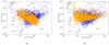 |
Fig. 1. P−Ṗ diagram of the simulated population, along with the observations, including both gamma-ray and radio pulsars. (a) Decaying magnetic field case. (b) Constant magnetic field case. |
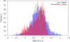 |
Fig. 2. Distribution of the observed period taken from the ATNF catalogue, along with the simulations. |
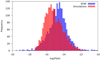 |
Fig. 3. Distribution of the observed period derivative Ṗ taken from the ATNF catalogue, along with the simulations. |
4.2. Pulsar types
We compute the total number Nr, Ng, and Nrg, which are the number of radio-only, gamma-only, and radio-loud gamma-ray pulsars, respectively, and within the energy bands  W and
W and  W. The resulting numbers are within the observations, and are better constrained by the decaying magnetic field model (see Tables 3 and 4). We represent the P−Ṗ diagram for Nr, Ng and Nrg in Figs. 4–6 for both the simulations and the observations. We find good agreement between the observed and simulated population separately for each sub-class.
Quantities Nr, Ng, and Nrg are the number of radio-only, gamma-only, and radio-loud gamma-ray pulsars, respectively, obtained from our simulations for a constant magnetic field.
Quantities Nr, Ng, and Nrg are the number of radio-only, gamma-only, and radio-loud gamma-ray pulsars, respectively, obtained from our simulations with a decaying magnetic field.
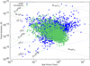 |
Fig. 4. P−Ṗ diagram of the radio-only pulsars for both the simulations and the observations. |
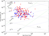 |
Fig. 5. P−Ṗ diagram of the gamma-only pulsars for both the simulations and the observations. |
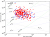 |
Fig. 6. P−Ṗ diagram of the radio-loud gamma ray pulsars for both the simulations and the observations. |
4.3. Spatial distribution
The distances d from Earth to the detected pulsars are shown in Fig. 7 for both the simulations and the observations. We find that more pulsars are detected at closer distances, and less at further distances. The projected 2D distribution is shown in Fig. 8, which represents the Galactic coordinate y as a function of x. As was mentioned earlier, since we detect more pulsars with low  , we detect more pulsars that are closer to us (see Eq. (26)). The distribution of the latitude for the simulated and observed population is shown in Fig. 9. In our simulations, we detect fewer pulsars at a lower Galactic latitude. This is due to the spatial distribution of pulsars, which shows pulsars closer to the Sun compared to observations, and therefore artificially increases their latitude. This may indicate that a more refined treatment of the sensibility depending on the latitude, and a better description of the initial spatial distribution as well as the birth kick velocity, should be implemented. Furthermore, our current simulation does not take into account the Galactic potential. The simulated pulsars’ latitude spreads would shift more towards the Galactic plane, thus increasing the number of pulsars in lower Galactic latitudes, and perhaps better representing the data.
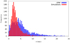 |
Fig. 7. Distribution of the distance to Earth for the simulated and observed populations. |
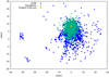 |
Fig. 8. Detected and observed spatial distribution of pulsars projected onto the Galactic plane. |
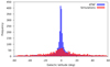 |
Fig. 9. Distribution of the observed Galactic latitude, b, in degrees, taken from the ATNF catalogue, along with the simulations. |
4.4. Influence of the parameters
Here we want to show the influence of the parameters on the quantities Nr, Ng, and Nrg, which are the number of radio only, gamma only, and radio-loud gamma-ray pulsars, respectively, from our simulations with the parameters given in Table 2. This is summarized in Tables 5–10. The most sensitive parameters are the birth rate, the initial mean magnetic field, and σb.
Influence of the birth rate on the quantities Nr, Ng, and Nrg.
Influence of the initial period on the quantities Nr, Ng, Nrg.
Influence of the σP on the Nr, Ng, and Nrg.
Influence of σb on the quantities Nr, Ng, and Nrg.
Influence of the S/N on the quantities Nr, Ng, and Nrg.
First the number of detected pulsars Ntot scales linearly with the birth rate τbirth. Increasing the birth rate by a factor of two decreases Ntot by the same factor. We indeed detect statistically more pulsars if more are present within our Galaxy. This trend is clearly seen for the rates 1/50 yr, 1/100 yr, and 1/200 yr (see Table 5).
The mean magnetic field also drastically impacts Ntot. The number of detected pulsars decreases with increasing field strength (Table 6). This is mainly due to the fact that high magnetic pulsars align faster than low magnetic field pulsars. Furthermore, the magnetic field decay is also faster for higher magnetic fields.
The initial mean period moderately impacts the detected pulsar number, as shown in Table 7. Increasing this period by a factor of ten only increases Ntot by a factor of two. Moreover, Ntot remains insensitive to the spread in this birth period (see Table 8).
Increasing the spread in magnetic field strength allows for lower B field values and, as seen above, a larger number of pulsars will be detected (Table 9). In this paper, we use S/N = 10 to get the detected pulsars, but in reality pulsars have been detected with telescopes having different sensitivities. Table 10 allows us to better understand how the detection changes with the S/N.
Decreasing the S/N naturally increases the number of detected pulsars. For instance, switching from S/N = 10 to S/N = 5 multiplies the number of detected pulsars by a factor of 1.7.
4.5. Radio width wr as a function of the period
Figure 10 represents the logarithm of the width of the radio pulse profile log(wr) as a function of the logarithm of the period log(P), to compare our simulations with the data. We retrieve the trend shown in the observations, namely a decrease of the width with an increase in the period. The slope in log-log scale is −0.53 ± 0.02, meaning wr = (1.04 ± 0.01)P−0.53 ± 0.02 as expected by the emission cone model. A linear fit to the measured pulsar width data from Posselt et al. (2021) gives w10 = (1.17 ± 0.01)P−0.34 ± 0.03, which, although indicative of the expected trend, still does not agree with the index of ∼ − 0.5. We believe that a more robust analysis and a larger data set will be more appropriate to verify the width period relation, which is beyond the scope of this work. However, although expected from geometrical considerations, no small values for wr have been obtained, particularly for faster periods. This may be explained by the fact that fast rotating pulsars usually show a larger opening angle for the emission beam, naturally leading to a broadening of the pulse profile.
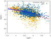 |
Fig. 10. log(wr) as a function of log(P). The quantity wr is expressed in degrees and P is expressed in s. The data are the width at the 10% level taken from Posselt et al. (2021). The solid blue line and the shaded area represent the result of a linear fit to the data and its uncertainties, and the solid red line and the shaded area represent a linear fit to the simulations, with its uncertainties. |
4.6. Inclination angle
Figure 11 shows the initial obliquity cos(α0) at birth and the current obliquity cos(α) distribution of the pulsars, irrespective of their detection. Most of the pulsars tend to the aligned configuration when aging. This is due to the fact that older pulsars are in larger number and are more likely to be aligned. Indeed, Fig. 12 highlights that most of the detected pulsars in our sample are older than 106 yr. This is expected since the birth rate is constant up to Gyr. Figure 13 shows the distributions of initial cos(α0) and current cos(α) obliquity for the detected pulsars. The current obliquity distribution cosα is almost uniform, whereas the distribution at birth cos(α0) peaks for values less than 0.4. This means that mostly only pulsars with larger initial inclination angles, close to orthogonal rotators, will be detected. Moreover, the alignment timescale is longer for high obliquities, meaning small cosα0 (see Fig. 14). Since the pulsed emission becomes harder to detect when the pulsar approaches an aligned rotator, pulsars with a longer alignment timescale are favoured, and therefore there is a bias towards small cosα0.
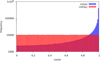 |
Fig. 11. Distribution of cosα and cosα0 for a sub-sample of 106 simulated population (‘before’ the detection). |
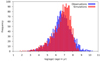 |
Fig. 12. Age distribution of the detected and observed pulsars. |
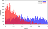 |
Fig. 13. Distribution of cos(α) and cosα0 for the ‘detected’ pulsars. |
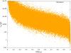 |
Fig. 14. Alignment timescale, |

5. Discussion
Population synthesis of neutron stars represents a valuable and reliable tool to constrain the basic physics of neutron star electrodynamics, from its surface up to large distances well outside the light cylinder. Following the work of Gullón et al. (2014), we have shown that a realistic pulsar model such as the force-free evolution scenario can self-consistently account for the observed population of canonical pulsars, and thus verified the findings of Gullón et al. (2014). Additionally, we have considered the sub-population of gamma-ray pulsars associated with the striped wind emission model. We find a birth rate of 1/70 yr, which is consistent with previous studies (Gonthier et al. 2004; Watters & Romani 2011). In the case of a constant magnetic field, we find that a birth rate of 1/300 yr improves the matching to the observations. However, this value is not consistent with expectations from previous works. The best results are obtained with a decaying magnetic field model.
In our study, we focused only on canonical pulsars for several reasons. First, the radio emission height and geometry were well constrained only for pulsars with periods P > 20 ms. Second, the binary pulsars were mostly revived through an accretion phase that was not included in our model. Third, magnetars with super-critical magnetic field strengths require a special initial magnetic field distribution, deviating from the normal canonical pulsar population we used. These magnetars are probably produced by a dynamo effect right at their birth during the proto-neutron star stage, increasing their internal magnetic field by several orders of magnitude through turbulent motion or magneto-rotational instabilities. Although achievable, we did not include such processes that would lead to a second distribution of magnetic field strengths designed especially for magnetars.
The spatial distribution of neutron stars at birth was postulated and adapted from the literature to fit as well as possible the current observed Galactic distribution, taking into account selection effects related to the sensitivity of radio and high energy telescopes. We found a reasonable agreement between the current spatial distribution and the simulated distribution.
The radio emission geometry constrained by the dipolar region combined with the striped wind emission model for gamma-rays are able to reproduce the entire population of young pulsars summarized in the P−Ṗ diagram. The number of radio only, gamma-ray only, or radio-loud gamma-ray pulsars fits the observed population as given by the ATNF catalogue. In a previous study, Pétri & Mitra (2021) demonstrated that the radio-loud gamma-ray pulsar emission model accurately constrained the geometry of the magnetic axis and line of sight axis with respect to the rotation axis. In this paper, we went one step further, showing that our model is consistent with the entire canonical pulsar population.
There are few other selection effects that can affect the detection of a neutron star in the same way as a radio pulsar, and we have not included these in our analysis. One such selection effect is the propagation of the radio signal in the ISM, which is subject to a scattering effect that smears out the signal, rendering the detection of some pulsars very difficult because the pulsation disappears at low frequencies. Interstellar scattering is associated with the fluctuation of the electron distribution along the observer’s line of sight, where the pulsar signal suffers a multi-path scattering as the signal traverses the ISM, (see Scheuer 1968). The scattering effect, therefore, can be described as the pulse width to be convolved with the response function of the ISM, and as a result the observed pulse width appears to be smeared. If the smearing exceeds the pulse period, then the pulsar cannot be detected as a pulsed signal. The effect of scattering is known to increase with pulsar dispersion measure (see, e.g., Krishnakumar et al. 2015) and hence, also the distance. Thus, the farther the pulsars, the more difficult they becomes to detect. The scattering timescale is a strong function of the observing frequency ν with the timescale decreasing as ∼ν−4.4 (see, e.g., Löhmer et al. 2004), hence sensitive pulsar searches at higher frequencies can in principle be used to detect more pulsars. However, due to steep radio pulsar spectra, pulsars are weaker at higher frequencies, and thus it may not be viable to detect a highly scattered pulsar.
The other selection effect is related to the coherent radio emission mechanism for radio pulsars. Our analysis here considers the geometrical model of a star centred magnetic dipole for the radio pulsars. However, the condition under which the radio emission mechanism can operate in pulsars are not included. Various studies suggest that the presence of a surface multi-polar field facilitates the generation of pair plasma, which in turn can assist mechanisms of coherent radio emission. Thus, the nature of the multi-polar surface field can affect the number of detectable pulsars, and several studies suggest a death-line in the P−Ṗ diagram (see e.g., Chen & Ruderman 1993; Mitra et al. 2020). In the current study, however, the pulsars detected via simulations are similar to the actual pulsars, and thus the above selection effects do not appear to have any major impact on the number of detected pulsars.
6. Summary
In this paper, we have shown that the secular evolution of the neutron star spin rate and its braking is accurately captured by the force-free magnetosphere model, in which radio photons emanate from regions near the polar cap, whereas the gamma-ray photons are produced within the current sheet of the striped wind. Following simple prescriptions for the birth kick, the birth period, and the birth magnetic field strength, assuming an isotropic obliquity and an isotropic viewing angle, we were able to pin down the essential parameters of the canonical pulsar population. Almost orthogonal rotators at birth represent the vast majority of pulsars currently detected due to the alignment effect, the geometry of the radio, and gamma-ray beams.
Our investigation could be improved in several ways, as exposed in the previous Sect. 5. Moreover, knowing the geometry of each individual pulsar, we could model the thermal X-ray emission from the polar caps, for instance for PSR J1136+1551 (Pétri & Mitra 2020). The upcoming advent of the SKA telescope will increase by one order of magnitude the number of known pulsars and constrain even further the evolution scenario and emission physics of these stellar remnants.
According to the ATNF catalogue at https://www.atnf.csiro.au/research/pulsar/psrcat/
Defined here as the pulsars that are non-binaries, with P > 20 ms and that are not magnetars.
Acknowledgments
This work has been supported by the CEFIPRA grant IFC/F5904-B/2018 and ANR-20-CE31-0010. We acknowledge the High Performance Computing Centre of the University of Strasbourg for supporting this work by providing scientific support and access to computing resources. We thank David Smith for stimulating discussions. DM acknowledges the support of the Department of Atomic Energy, Government of India, under project no. 12-R&D-TFR-5.02-0700.
References
- Abdo, A. A., Ajello, M., Allafort, A., et al. 2013, ApJS, 208, 17 [Google Scholar]
- Arons, J. 1983, ApJ, 266, 215 [CrossRef] [Google Scholar]
- Binney, J., & Merrifield, M. 1998, Galactic Astron. [Google Scholar]
- Bogdanov, S., Lamb, F. K., Mahmoodifar, S., et al. 2019, ApJ, 887, L26 [NASA ADS] [CrossRef] [Google Scholar]
- Chen, K., & Ruderman, M. 1993, ApJ, 402, 264 [NASA ADS] [CrossRef] [Google Scholar]
- Cheng, K. S., Ho, C., & Ruderman, M. 1986, ApJ, 300, 500 [CrossRef] [Google Scholar]
- Cordes, J. M., Freire, P. C. C., Lorimer, D. R., et al. 2006, ApJ, 637, 446 [NASA ADS] [CrossRef] [Google Scholar]
- Coroniti, F. V. 1990, ApJ, 349, 538 [Google Scholar]
- Daugherty, J. K., & Harding, A. K. 1982, ApJ, 252, 337 [NASA ADS] [CrossRef] [Google Scholar]
- Daugherty, J. K., & Harding, A. K. 1996, ApJ, 458, 278 [NASA ADS] [CrossRef] [Google Scholar]
- Deutsch, A. J. 1955, Ann. Astrophys., 18, 1 [NASA ADS] [Google Scholar]
- Faucher-Giguère, C.-A., & Kaspi, V. M. 2006, ApJ, 643, 332 [CrossRef] [Google Scholar]
- Goldreich, P., & Julian, W. H. 1969, ApJ, 157, 869 [Google Scholar]
- Gonthier, P. L., Ouellette, M. S., Berrier, J., O’Brien, S., & Harding, A. K. 2002, ApJ, 565, 482 [NASA ADS] [CrossRef] [Google Scholar]
- Gonthier, P. L., Van Guilder, R., & Harding, A. K. 2004, ApJ, 604, 775 [NASA ADS] [CrossRef] [Google Scholar]
- Gonthier, P. L., Harding, A. K., Ferrara, E. C., et al. 2018, ApJ, 863, 199 [NASA ADS] [CrossRef] [Google Scholar]
- Gullón, M., Miralles, J. A., Viganò, D., & Pons, J. A. 2014, MNRAS, 443, 1891 [CrossRef] [Google Scholar]
- Harding, A. K., & Muslimov, A. G. 2011, ApJ, 743, 181 [NASA ADS] [CrossRef] [Google Scholar]
- Harding, A. K., Stern, J. V., Dyks, J., & Frackowiak, M. 2008, ApJ, 680, 1378 [NASA ADS] [CrossRef] [Google Scholar]
- Hirotani, K. 2008, ApJ, 688, L25 [NASA ADS] [CrossRef] [Google Scholar]
- Hobbs, G., Lorimer, D. R., Lyne, A. G., & Kramer, M. 2005, MNRAS, 360, 974 [Google Scholar]
- Jackson, J. D. 2001, Électrodynamique classique : Cours et exercices d’électromagnétisme (Paris: Dunod) [Google Scholar]
- Johnston, S., Smith, D. A., Karastergiou, A., & Kramer, M. 2020, MNRAS, 497, 1957 [NASA ADS] [CrossRef] [Google Scholar]
- Kalapotharakos, C., Harding, A. K., & Kazanas, D. 2014, ApJ, 793, 97 [Google Scholar]
- Kalapotharakos, C., Harding, A. K., Kazanas, D., & Brambilla, G. 2017, ApJ, 842, 80 [NASA ADS] [CrossRef] [Google Scholar]
- Kalapotharakos, C., Brambilla, G., Timokhin, A., Harding, A. K., & Kazanas, D. 2018, ApJ, 857, 44 [NASA ADS] [CrossRef] [Google Scholar]
- Kalapotharakos, C., Harding, A. K., Kazanas, D., & Wadiasingh, Z. 2019, ApJ, 883, L4 [NASA ADS] [CrossRef] [Google Scholar]
- Kirk, J. G., Skjæraasen, O., & Gallant, Y. A. 2002, A&A, 388, L29 [NASA ADS] [CrossRef] [EDP Sciences] [Google Scholar]
- Krishnakumar, M. A., Mitra, D., Naidu, A., Joshi, B. C., & Manoharan, P. K. 2015, ApJ, 804, 23 [NASA ADS] [CrossRef] [Google Scholar]
- Löhmer, O., Mitra, D., Gupta, Y., Kramer, M., & Ahuja, A. 2004, A&A, 425, 569 [NASA ADS] [CrossRef] [EDP Sciences] [Google Scholar]
- Lorimer, D. R., & Kramer, M. 2004, Handbook of Pulsar Astronomy [Google Scholar]
- Lorimer, D. R., Faulkner, A. J., Lyne, A. G., et al. 2006, MNRAS, 372, 777 [NASA ADS] [CrossRef] [Google Scholar]
- Lyne, A. G., Manchester, R. N., & Taylor, J. H. 1985, MNRAS, 213, 613 [NASA ADS] [CrossRef] [Google Scholar]
- Manchester, R. N., Lyne, A. G., Camilo, F., et al. 2001, MNRAS, 328, 17 [NASA ADS] [CrossRef] [Google Scholar]
- Manchester, R. N., Hobbs, G. B., Teoh, A., & Hobbs, M. 2005, AJ, 129, 1993 [Google Scholar]
- Mdzinarishvili, T. G., & Melikidze, G. I. 2004, A&A, 425, 1009 [NASA ADS] [CrossRef] [EDP Sciences] [Google Scholar]
- Michel, F. C. 1994, ApJ, 431, 397 [Google Scholar]
- Michel, F. C., & Goldwire, H. C. Jr. 1970, Astrophys. Lett., 5, 21 [NASA ADS] [Google Scholar]
- Mitra, D. 2017, J. Astrophys. Astron., 38, 52 [NASA ADS] [CrossRef] [Google Scholar]
- Mitra, D., Basu, R., Melikidze, G. I., & Arjunwadkar, M. 2020, MNRAS, 492, 2468 [NASA ADS] [CrossRef] [Google Scholar]
- Muslimov, A. G., & Harding, A. K. 2004, ApJ, 617, 471 [NASA ADS] [CrossRef] [Google Scholar]
- Paczynski, B. 1990, ApJ, 348, 485 [NASA ADS] [CrossRef] [Google Scholar]
- Pétri, J. 2009, A&A, 503, 13 [NASA ADS] [CrossRef] [EDP Sciences] [Google Scholar]
- Pétri, J. 2011a, MNRAS, 412, 1870 [Google Scholar]
- Pétri, J. 2011b, A unified polar cap/striped wind model for pulsed radio and gamma-ray emission in pulsars, physics of Neutron Stars, Saint-Petersbourg, Russie [Google Scholar]
- Pétri, J. 2012, MNRAS, 424, 605 [Google Scholar]
- Pétri, J. 2016, MNRAS, 455, 3779 [Google Scholar]
- Pétri, J., & Mitra, D. 2020, MNRAS, 491, 80 [Google Scholar]
- Pétri, J., & Mitra, D. 2021, A&A, 654, A106 [NASA ADS] [CrossRef] [EDP Sciences] [Google Scholar]
- Philippov, A., Tchekhovskoy, A., & Li, J. G. 2014, MNRAS, 441, 1879 [NASA ADS] [CrossRef] [Google Scholar]
- Pierbattista, M., Grenier, I. A., Harding, A. K., & Gonthier, P. L. 2012, A&A, 545, A42 [NASA ADS] [CrossRef] [EDP Sciences] [Google Scholar]
- Popov, S. B., Pons, J. A., Miralles, J. A., Boldin, P. A., & Posselt, B. 2010, MNRAS, 401, 2675 [NASA ADS] [CrossRef] [Google Scholar]
- Posselt, B., Karastergiou, A., Johnston, S., et al. 2021, MNRAS, 508, 4249 [NASA ADS] [CrossRef] [Google Scholar]
- Ravi, V., Manchester, R. N., & Hobbs, G. 2010, ApJ, 716, L85 [Google Scholar]
- Riley, T. E., Watts, A. L., Bogdanov, S., et al. 2019, ApJ, 887, L21 [Google Scholar]
- Ruderman, M. A., & Sutherland, P. G. 1975, ApJ, 196, 51 [Google Scholar]
- Scheuer, P. A. G. 1968, Nature, 218, 920 [NASA ADS] [CrossRef] [Google Scholar]
- Siegert, T. 2019, A&A, 632, L1 [NASA ADS] [CrossRef] [EDP Sciences] [Google Scholar]
- Smith, D. A., Bruel, P., Cognard, I., et al. 2019, ApJ, 871, 78 [NASA ADS] [CrossRef] [Google Scholar]
- Spitkovsky, A. 2006, ApJ, 648, L51 [Google Scholar]
- Sturrock, P. A. 1971, ApJ, 164, 529 [Google Scholar]
- Takata, J., Wang, Y., & Cheng, K. S. 2011, ApJ, 726, 44 [Google Scholar]
- Taylor, J. H., & Manchester, R. N. 1977, ApJ, 215, 885 [NASA ADS] [CrossRef] [Google Scholar]
- Thompson, D. J., Bertsch, D. L., Dingus, B. L., et al. 1995, ApJS, 101, 259 [NASA ADS] [CrossRef] [Google Scholar]
- van der Kruit, P. C. in Comparison of the Galaxy with External Spiral Galaxies, eds. G. Gilmore, & B. Carswell (Dordrecht: Springer, Netherlands), 27 [Google Scholar]
- Viganò, D. 2013, ArXiv e-prints [arXiv:1310.1243] [Google Scholar]
- Viganò, D., Rea, N., Pons, J. A., et al. 2013, MNRAS, 434, 123 [CrossRef] [Google Scholar]
- Watters, K. P., & Romani, R. W. 2011, ApJ, 727, 123 [NASA ADS] [CrossRef] [Google Scholar]
- Yadigaroglu, I.-A., & Romani, R. W. 1995, ApJ, 449, 211 [NASA ADS] [CrossRef] [Google Scholar]
All Tables
Quantities Nr, Ng, and Nrg are the number of radio-only, gamma-only, and radio-loud gamma-ray pulsars, respectively, obtained from our simulations for a constant magnetic field.
Quantities Nr, Ng, and Nrg are the number of radio-only, gamma-only, and radio-loud gamma-ray pulsars, respectively, obtained from our simulations with a decaying magnetic field.
All Figures
|
Fig. 1. P−Ṗ diagram of the simulated population, along with the observations, including both gamma-ray and radio pulsars. (a) Decaying magnetic field case. (b) Constant magnetic field case. |
| In the text | |
|
Fig. 2. Distribution of the observed period taken from the ATNF catalogue, along with the simulations. |
| In the text | |
|
Fig. 3. Distribution of the observed period derivative Ṗ taken from the ATNF catalogue, along with the simulations. |
| In the text | |
|
Fig. 4. P−Ṗ diagram of the radio-only pulsars for both the simulations and the observations. |
| In the text | |
|
Fig. 5. P−Ṗ diagram of the gamma-only pulsars for both the simulations and the observations. |
| In the text | |
|
Fig. 6. P−Ṗ diagram of the radio-loud gamma ray pulsars for both the simulations and the observations. |
| In the text | |
|
Fig. 7. Distribution of the distance to Earth for the simulated and observed populations. |
| In the text | |
|
Fig. 8. Detected and observed spatial distribution of pulsars projected onto the Galactic plane. |
| In the text | |
|
Fig. 9. Distribution of the observed Galactic latitude, b, in degrees, taken from the ATNF catalogue, along with the simulations. |
| In the text | |
|
Fig. 10. log(wr) as a function of log(P). The quantity wr is expressed in degrees and P is expressed in s. The data are the width at the 10% level taken from Posselt et al. (2021). The solid blue line and the shaded area represent the result of a linear fit to the data and its uncertainties, and the solid red line and the shaded area represent a linear fit to the simulations, with its uncertainties. |
| In the text | |
|
Fig. 11. Distribution of cosα and cosα0 for a sub-sample of 106 simulated population (‘before’ the detection). |
| In the text | |
|
Fig. 12. Age distribution of the detected and observed pulsars. |
| In the text | |
|
Fig. 13. Distribution of cos(α) and cosα0 for the ‘detected’ pulsars. |
| In the text | |
|
Fig. 14. Alignment timescale, |
| In the text | |
Current usage metrics show cumulative count of Article Views (full-text article views including HTML views, PDF and ePub downloads, according to the available data) and Abstracts Views on Vision4Press platform.
Data correspond to usage on the plateform after 2015. The current usage metrics is available 48-96 hours after online publication and is updated daily on week days.
Initial download of the metrics may take a while.