| Issue |
A&A
Volume 695, March 2025
|
|
|---|---|---|
| Article Number | A153 | |
| Number of page(s) | 12 | |
| Section | Planets, planetary systems, and small bodies | |
| DOI | https://doi.org/10.1051/0004-6361/202452749 | |
| Published online | 19 March 2025 | |
Physically motivated analytic model of energy efficiency for extreme-ultraviolet-driven atmospheric escape of close-in exoplanets
1
Faculty of Physics, University of Duisburg-Essen,
Lotharstraße 1,
47057
Duisburg, Germany
2
Department of Physics, School of Science, The University of Tokyo,
7-3-1 Hongo,
Bunkyo, Tokyo
113-0033, Japan
3
Dipartimento di Fisica, Università degli Studi di Milano,
Via Celoria, 16,
20133
Milano, Italy
★ Corresponding author; hiroto.mitani@uni-due.de
Received:
25
October
2024
Accepted:
11
February
2025
Extreme-ultraviolet (EUV) driven atmospheric escape is a key process in the atmospheric evolution of close-in exoplanets. In many evolutionary models, an energy-limited mass-loss rate with a constant efficiency (typically ∼10%) is assumed for calculating the mass-loss rate. However, hydrodynamic simulations have demonstrated that this efficiency depends on various stellar and planetary parameters. Comprehending the underlying physics of the efficiency is essential for understanding planetary atmospheric evolution and recent observations of the upper atmosphere of close-in exoplanets. We introduce relevant temperatures and timescales derived from physical principles to elucidate the mass-loss process. Our analytical mass-loss model is based on phenomenology and consistent across a range of planetary parameters. We compared our mass-loss efficiency with that of radiation hydrodynamic simulations, finding that our model can predict efficiency in both energy-limited and recombination-limited regimes. We further applied our model to exoplanets observed with hydrogen absorption (Lyα and Hα). Our findings suggest that Lyα absorption is detectable in planets subjected to intermediate EUV flux; under these conditions, the escaping outflow is insufficient in low-EUV environments, while the photoionization timescale remains short in high EUV ranges. Conversely, Hα absorption is detectable under high-EUV-flux conditions, facilitated by the intense Lyα flux exciting hydrogen atoms. According to our model, the non-detection of neutral hydrogen can be explained by a low mass-loss rate and is not necessarily due to stellar wind confinement or the absence of a hydrogen-dominated atmosphere in many cases. This model can help identify future observational targets and explicates the unusual absorption detection/non-detection patterns observed in recent studies.
Key words: planets and satellites: atmospheres / planets and satellites: gaseous planets / planets and satellites: general
© The Authors 2025
 Open Access article, published by EDP Sciences, under the terms of the Creative Commons Attribution License (https://creativecommons.org/licenses/by/4.0), which permits unrestricted use, distribution, and reproduction in any medium, provided the original work is properly cited.
This article is published in open access under the Subscribe to Open model. Subscribe to A&A to support open access publication.
1 Introduction
Extreme ultraviolet (EUV) radiation, with energy greater than approximately 13.6 eV, from host stars plays a critical role in heating the upper atmospheres of close-in exoplanets. This occurs through the photoionization of hydrogen atoms. Such heating is a key driver of hydrodynamic escape (Lammer et al. 2003; Yelle 2004; Murray-Clay et al. 2009; Owen & Jackson 2012; Kubyshkina et al. 2018b), which significantly impacts the evolution of close-in exoplanets and influences various exo-planetary characteristics, such as the sub-Jovian desert and mass-radius gap (Kurokawa & Nakamoto 2014; Mazeh et al. 2016; Fulton et al. 2017; Owen & Wu 2017; Gupta & Schlichting 2019). Numerous transit observations have detected escaping atmospheres around close-in exoplanets, typically through Lyα absorption due to its large transit depth (Vidal-Madjar et al. 2003; Lecavelier Des Etangs et al. 2010; Kulow et al. 2014; Ehrenreich et al. 2015). More recent studies have also used Hα (e.g., Cauley et al. 2017; Yan et al. 2021) and the helium triplet (e.g., Oklopčić & Hirata 2018; Spake et al. 2018; Allart et al. 2023) to observe upper atmospheres using ground-based telescopes. Despite the intense radiation expected to heat these upper atmospheres and drive hydrodynamic escape, some closein planets show no helium absorption (Bennett et al. 2023; Allart et al. 2023). This absence could be explained by several factors: the planets might have already lost their hydrogen-dominated atmospheres (e.g., Zhang et al. 2022), strong stellar winds could be confining the atmospheres and reducing absorption signals (Carolan et al. 2020; Mitani et al. 2022), or the escaping outflow might be insufficient due to low EUV flux. Understanding the physics behind the atmospheric thermochemical structure is crucial for interpreting these observational trends.
There are several types of hydrodynamic escape driven by radiation from the host stars (Murray-Clay et al. 2009; Owen 2019). If the radiation is not intense, the system becomes energy-limited and the mass-loss rate of the atmosphere is almost proportional to the flux of EUV radiation. Conversely, in the presence of intense ultraviolet radiation, radiative cooling regulates the gas temperature and the system becomes recombination-limited. In this regime, the mass-loss efficiency decreases, and the mass-loss rate is not proportional to the flux but is nearly proportional to the square root of the flux. The energy efficiency varies with the escape regime and shapes the history of planetary mass loss. In many simulations of planetary evolution, an energy-limited mass-loss rate with a constant efficiency is assumed (e.g., Lopez & Fortney 2013; Fujita et al. 2022). However, this simplification overlooks the variability in the efficiency, which depends on several stellar and planetary parameters and thus does not remain constant. To improve the accuracy of planetary evolution models, it is necessary to understand the criteria that determine this efficiency. The physical conditions that govern these regimes are not well understood but are known to depend on the planetary mass, radius, surface temperature/density, orbital distance, stellar mass, stellar EUV luminosity, and EUV spectral hardness. Previous analytical models (Kubyshkina et al. 2018a) were based on a fit to simulations and did not derive these dependences from a first-principles approach. The recent analytical model of hydrogen tails and observational signatures from Owen et al. (2023) has shown the dependence of photoionization and mass-loss outflow on the observational absorption depth, treating the mass-loss rate as a free parameter.
We have developed an analytical model of the mass-loss rates in a first-principle approach to deepen our understanding of the physics of EUV-driven atmospheric escape that depends on basic stellar and planetary parameters. We examined the physical conditions to analytically characterize the environment and establish simple criteria that can be used for planetary evolution models and for interpreting observations of atmospheric escape.
In Sect. 2, we outline the physical timescales and temperatures that govern the physics of atmospheric escape driven by EUV photoionization heating. In Sect. 3, we present the analytic mass-loss rate and mass-loss efficiency applicable across a general parameter range, including energy-limited and recombination-limited regimes. In Sect. 4, we provide the comparison between our model and observed close-in planets. In Sect. 5, we discuss our model further and in Sect. 6 present our conclusions.
2 Essential parameters
The dynamical and thermal state of the EUV-driven escaping gas is essentially governed by photo-heating and gravity. To investigate the basic physics of EUV-driven atmospheric escape, we introduced key quantities that describe these physical effects.
We defined the characteristic temperature, Tch (Woods et al. 1996; Begelman et al. 1983; Nakatani et al. 2024) for a measure of the magnitude of photo-heating as
 (1)
(1)
where ΓEUV represents the specific EUV photo-heating rate, RHill is the Hill radius, REUV is the effective planetary radius where the optical depth to EUV photons is unity,  is the Bondi radius where cs is the isothermal sound speed of the atmosphere, k is the Boltzmann constant, cp = γ/(γ − 1) is the normalized specific heat at constant pressure with the specific heat ratio γ, µ is the mean molecular weight, cch is the sound speed of the gas at the characteristic temperature, and mH is the hydrogen atomic mass. We note that the sound speed cch on the right-hand side (RHS) depends on the characteristic temperature Tch . The RHS represents the total deposited photo-energy within the typical sound crossing time. We used min(RHill, Rs) − REUV as the typical length scale of the streamline where the bulk of heating occurs, as the photo-heating outside the sonic point does not affect the thermal structure within the sonic point and if the Hill radius is smaller than the Bondi radius, the stellar gravity boosts the gas velocity to sonic speed around the Hill radius. Hence, the characteristic sound speed is defined as

where R′p = min(RHill, RB) − REUV. The characteristic temperature indicates how rapid the photo-heating is compared to the dynamical timescale but does not necessarily give the typical temperature of the photo-heated gas. For instance, under conditions of high EUV irradiation, the characteristic temperature may exceed a million kelvins. However, the actual atmospheric temperature is kept lower due to radiative cooling processes, which effectively limit the gas temperature. In such a planet with a high characteristic temperature, the fraction of the neutral hydrogen is not unity and the characteristic temperature should be lowered. However, the gas temperature reaches the equilibrium temperature as demonstrated in Sect. 3.1 and the characteristic temperature as in Eq. (1) is practically useful to understand the gas temperature.
The heating timescale th is defined as

where h is the specific enthalpy. The specific heating rate ΓEUV is
 (2)
(2)
where m denotes the gas mass per hydrogen nucleus, σν is the absorption cross section of neutral hydrogen for EUV frequency ν, yHI is the atomic hydrogen abundance, and δ is the ratio of the attenuated flux to the unattenuated flux (Fν,0) at a given H I column density (NHI),

Here, ⟨σ⟩ is the average cross section of the ionizing photons reaching NHI ,

and ⟨∆E⟩i is the average deposited energy per ionization at NHI,

where Φν is the specific stellar EUV emission rate and r is the distance to the planet from the host star. The terms δ, ⟨σ⟩, and ⟨E⟩i are only dependent on NHI and a priori calculable, given the EUV spectrum. The first two are monotonically decreasing functions, while the third is a monotonically increasing function. The product δ⟨σ⟩⟨E⟩i is a monotonically decreasing function with respect to NHI, which is also evident by the NHI-derivative of ΓEUV. For convenience later on, we defined  and
and  .
.
We can rewrite ΓEUV in Eq. (2) as
 (3)
(3)

The χe is a function of column density and the range is 0 to 1. In this study we neglected the attenuation because the atmospheric density structure is highly dependent on the radius. For realistic spectra, this assumption is not necessary but constructing a model based on the simplification is a step toward a full understanding of atmospheric escape driven by photo-heating and practically useful to understand the mass-loss rate of close-in exoplanets. Correspondingly, the characteristic sound speed is

where Φ is EUV luminosity of the host star.
From the balance of photo-heating and cooling, the gas has an equilibrium temperature Teq, which is typically ≈104 K for EUV-heated gas, with the corresponding sound speed ceq ≈ 10 km s−1. We note that the equilibrium temperature is not the planetary surface temperature, and that the atmospheric temperature cannot significantly exceed the equilibrium temperature. The equilibrium temperature may depend on the metal abundance of the atmosphere, as metal species serve as coolants. We discuss the effects of metallicity in Sect. 5.2.
The planetary gravity also plays an important role in the atmospheric escape process. The gravitational timescale is accordingly

We also defined the gravitational temperature,
 (4)
(4)
which characterizes the strength of planetary gravity and is compared with Teq and Tch . Essentially, the gas with temperatures hotter than Tg does not feel planetary gravity, and fast winds can be driven. If the characteristic temperature is lower than the gravitational temperature, the gas is significantly inhibited by gravity, and the winds tend to be subsonic (υgas < cg where υgas is the gas velocity and cg is the sound speed at the gravitational temperature) with temperatures on the order of the gravitational temperature, as discussed in Nakatani et al. (2024).
The neutral hydrogen fraction also plays a crucial role in interpreting the observed hydrogen absorption. The balance between photoionization and recombination determines the neutral hydrogen fraction because the dynamical timescale is usually longer than the photoionization timescale in the case of closein exoplanets. We can define the photoionization/recombination timescales as
 (5)
(5)
 (6)
(6)
where tion is the photoionization timescale, trec denotes the recombination timescale, and nH is the number density of hydrogen atoms. αrec ~ 2.7 × 10⁻¹³ cm3/s is the radiative recombination rate coefficient for hydrogen ions. The recombination coefficient is temperature-dependent; however, in many cases, we find that this dependence has a minimal impact on our results. This is primarily because the recombination coefficient scales approximately with the square root of temperature, meaning that temperature variations result in only minor adjustments to the ratio of the relevant timescales. It is important to note that the photoionization timescale is influenced by the EUV flux (which is a function of both EUV luminosity and orbital distance), while the recombination timescale is determined by the gas density. For planetary outflows, these calculations can be based on the physical conditions at the base of the flow. Up to this point, we have introduced th , tion , tg , and trec as relevant timescales, Tch , Teq, and Tg as relevant temperatures, and cch , cg , and ceq as relevant sound speeds.
If Tch > Teq, photo-heating is so rapid that it can increase the gas temperature Tgas to Teq before flowing out to a distance of ~Rhill. In this regime, Tgas ≈ Teq. The ratio between Tch and Teq is

where Rg is the gravitational radius defined as

The above ratio is rewritten as

where ξ = R′p/Rg. The second factor in the RHS defines the critical flux,


It should be noted that the Tch/Teq ratio determines the physical regime, while the critical EUV flux does not.
Similarly, the ratio of Tch to Tg is calculated as

Thus, the ratio of Rp to Rg determines whether the subspace where Tch > Teq also satisfies Tch > Tg, or vice versa. For relatively massive planets (Rg > Rp), the parameter space where Tch > Tg always satisfies Tch > Teq, implying that winds can be gravitationally inhibited even with temperatures of Teq.
3 Analytic model
Mass-loss rates determine the planetary evolution and the absorption signals. Understanding the basic physics of the massloss driven by EUV-photoionization is of use for, for example, finding the origins of peculiar observational signals. In this section we summarize our analytic model of mass-loss rates, which is built upon the essential parameters in Sect. 2 and physical conditions that govern the mass-loss efficiency. Our model is capable of seamlessly bridging between the energy-limited and recombination-limited mass-loss regimes. We provide the analytic formulae in Sect. 3.1. Additionally, we compare our model’s predictions with results from radiation hydrodynamic simulations in Sect. 3.2. This comparison helps validate our analytical approach and provides insights into the dynamics of atmospheric escape under various stellar and planetary conditions.
3.1 Mass-loss rates and efficiency
Mass loss driven by EUV photoionization heating is a crucial process in the evolution of close-in planets. Many planetary evolution studies rely on a simplified model where the mass-loss rate is calculated using an energy-limited formula (Watson et al. 1981; Erkaev et al. 2007):
 (8)
(8)
Here Ṁ represents the mass-loss rate, η is the efficiency of massloss, and K is the factor accounting for stellar gravity (Erkaev et al. 2007). While this formula provides a useful estimate, it usually assumes a constant efficiency (η), which simplifies the complex interplay of factors that can influence mass loss. In reality, η can vary significantly based on the planetary and stellar characteristics. In this section we formulate an analytic expression for the efficiency that depends on planetary and stellar parameters, using the relevant quantities introduced in Sect. 2.
In contrast to the energy-limited regime, radiative cooling plays an important role in the recombination-limited regime. In this regime, previous studies (Murray-Clay et al. 2009; Owen & Wu 2017) estimate the mass-loss rate by approximating the density profile within the sonic point to that in hydrostatic equilibrium:
 (9)
(9)
where Rs = RB, and fully ionized atmosphere (µ = 0.5) with the equilibrium temperature (Tgas = Teq,) are assumed to calculate the sound speed  has been applied instead of
  to account for the day-side illumination effect. The base density is given as nbase ~ (F0/αrecH)1/2 with H being the pressure scale height, which is defined as in Owen & Alvarez (2016):
![$H = \min \left[ {{{{R_{\rm{p}}}} \over 3},{{c_{\rm{s}}^2R_{\rm{p}}^2} \over {2G{M_{\rm{p}}}}}} \right].$](/articles/aa/full_html/2025/03/aa52749-24/aa52749-24-eq28.png) (10)
(10)
The base density formula, although originally derived under the assumption of a thin ionization front, primarily depends on the local recombination-ionization balance and the gas temperature rather than on the actual thickness of the front. Even with a thick ionization front, the gas near the base still reaches equilibrium between ionization and recombination if the recombination timescale is shorter than the flow timescale. The scale height depends on the gas temperature and we can estimate the base density not only for an atmosphere of 104 K, but also for a relatively low-temperature atmosphere. If the EUV flux is weak on a weak gravity planet, such as a sub-Neptune, this assumption is incorrect and the mass-loss rate gets overestimated.
In this model, the effect of stellar gravity is neglected. To ensure consistency across different mass-loss models, we similarly ignored stellar gravity when calculating the efficiency of mass loss. Specifically, we adopted the approximation K = 1 in our calculations to align with the simplifications inherent in the recombination-limited model. This approximation effectively assumes stellar gravity to be negligible. However, including the gravitational factor K in the planetary mass or radius does not significantly alter the results.
Essentially, our model updates Eq. (9) by incorporating the variations in the gas temperature Tgas , the ionization degree of gas, and the sonic point location Rs, which depend on the stellar and planetary parameters. We used a single representative temperature, neglecting the spatial temperature profile. We expressed the representative atmospheric temperature as follows:

This expression is derived from the following phenomenological considerations: the gas temperature does not exceed the equilibrium temperature due to the regulation by radiative cooling (Regime A-1); otherwise, the gas temperature, Tgas , is basically determined by a characteristic temperature, Tch (Regime A-2). On the other hand, if the photo-heating is weak enough to yield Tch lower than the gravitational temperature, Tg (Regime A-3), the deposited energy is charged to heat the gas to Tg at most. We note that, strictly speaking, Tg should be evaluated using REUV instead of Rp in Eq. (4). However, since Rp ≈ REUV in this regime, using Eq. (4) does not affect the results.
The revisions to Tgas also update the sound speed (cs) accordingly:
 (11)
(11)
where ceq , cch, and cg are the sound speeds at equilibrium temperature, characteristic temperature, and gravitational temperature, respectively (see Table 1). We note that cs depends on the mean molecular weight (µ) as well, which is determined once the ionization degree or, equivalently, the atomic hydrogen abundance is set. We approximated the atomic hydrogen abundance to min(tion/trec, 1), which in turn depends on cs through the scale height H incorporated in the base density. Hence, cs and µ must be determined simultaneously. The updates to Tgas and accordingly cs are summarized in Table 1 along with the corresponding parameter spaces.
As for the update to Rs , it does not necessarily coincide with the Bondi radius RB in general, as implicitly assumed in the classical model (Eq. (9)). In the parameter space where the Bondi radius exceeds the Hill radius RB > RHill, such as when the gas temperature is low or the stellar gravity is relatively strong, the stellar gravity becomes the primary accelerating source, and thus Rs ≈ RHill. In contrast, for the case where the Bondi radius approaches the wind-launching radius RB → REUV, meaning a high gas temperature or weak planetary gravity, the winds are instantly accelerated to be supersonic after being launched at the base REUV, resulting in Rs ≈ REUV. We note that we are not interested in the case where EUV photons fail to penetrate within the Hill radius, REUV > RHill , and that RB is constrained to not fall below REUV by definition (see Eq. (1)). We summarize the sonic point locations in Table 2.
The update to the sonic point locations results in two distinct expressions for Ṁ, depending on whether the sonic point Rs lies at the base REUV. If REUV < RB, the expression for Ṁ remains essentially the same as Eq. (9):
![${\dot M_1}\left( {{R_{\rm{s}}}} \right) = \pi R_{\rm{s}}^2{\upsilon _{{\rm{gas}}}}{m_{\rm{H}}}{n_{{\rm{base}}}}\exp \left[ {{{2{R_{\rm{B}}}} \over {{R_{{\rm{EUV}}}}}}\left( {{{{R_{{\rm{EUV}}}}} \over {{R_{\rm{s}}}}} - 1} \right)} \right].$](/articles/aa/full_html/2025/03/aa52749-24/aa52749-24-eq31.png) (12)
(12)
Here, we have replaced Rp in the original equation, Eq. (9), with REUV. On the contrary, for RB → REUV, REUV now serves as the sonic point, and Ṁ is updated to
 (13)
(13)
This equation is the asymptotic form of Eq. (12) when RB → REUV.
In Regimes A-1 and A-2, the gas velocity υg in Eqs. (12) and (13) is set to cs (Eq. (11)) as in the original equation (Eq. (9)). However, in Regime A-3 (gravity-inhibited regime), we applied an empirical correction factor based on the simulation results of our 1D simulations and ATES code to get more realistic massloss efficiencies for low EUV environments: υgas = cg(tg/th). This adjustment is necessary because using a single representative temperature Tg, while neglecting the spatial profile (1/r), is not valid in this regime, and the actual sound speed at the sonic point is significantly lower than the evaluated sound speed cg . Finally, the mass-loss rates of Eqs. (12) and (13) are fully determined once the effective planetary radius REUV is specified. We set this radius as the radius where the density of the isothermal atmosphere with the surface temperature becomes the base density:
 (14)
(14)
where RB is the Bondi radius based on the planetary surface temperature, and ρsurf is the density at the planet’s surface.
It should be noted that we neglected the spectral dependence of REUV, but the density structure of the inner atmosphere is strongly dependent on the radius. The cross-section dependence of REUV has a minor effect on the mass-loss rate.
By applying Eqs. (8), (12), and (13), we can semi-analytically calculate the mass-loss efficiency η across any given parameter space (see also Table 2). In Fig. 1, we present the calculated efficiencies for a fixed planetary mass. The conventional recombination-limited mass-loss rates sharply drop in regions of strong gravity (corresponding to smaller Rp , or equivalently smaller REUV in terms of Eq. (14)). This sharp decline is primarily due to a larger ratio of the sonic radius to the planetary radius, which causes the density at Rs to diminish exponentially (see Eq. (12)). The efficiency of the conventional recombination-limited model tends to overestimate the efficiency in environments characterized by weak gravity. In cases of a thick ionization front, the base density can be overestimated, which poses significant challenges for low-gravity and low-EUV flux planets. However, in such scenarios, the density profile becomes less steep with respect to the radius, thereby mitigating the impact of this overestimation. Our model tends to overestimate the mass-loss rate in these cases. However, the estimated sound speed compensates for this overestimation, unlike the conventional recombination-limited mass-loss rate.
We also compared our efficiency with that derived from 1D simulations (Caldiroli et al. 2021). We find that our efficiency more closely aligns with the simulation results in highly irradiated (FEUV > 104 erg/s/cm2) and relatively weak gravity (ϕp = GMp/Rp < 2 × 10¹³ erg/g) cases, compared to the conventional recombination-limited cases. The slightly decreasing trend in the efficiencies for larger planets is because η is proportional to  as in Eq. (8), with the mass-loss rate weakly depends on the radius (proportional to the square root of the radius as in Eq. (13) and ∝(1 − 2Rs/Rp) in Eq. (9) for larger Rp).
Next, we discuss the dependence of mass-loss efficiency on planetary mass. Figure 2 presents the planetary mass dependence of the efficiencies, similar to Fig. 1 but for a fixed planetary radius. The global trend is also akin to that can be found in Fig. 1; however, the dependence on gravity differs in high-irradiation and lower-gravity environments (left side of the curves), where the efficiency appears almost independent of planetary gravity. This is attributed to the gravity-dependent nature of the effective planetary radius, REUV (Eq. (14)). Efficiency η ∝ ṀMp, and both REUV and the mass-loss rate increase for lower-mass planets. Near Mp ∼ MJ, the Bondi radius approaches the Hill radius. We also find that the Hill radius affects the efficiency slightly (<10%) for high-mass planets (Mp > MJ).
For strong-gravity planets with intense EUV radiation (Rp < RJ, Mp > MJ, and FEUV > 105 erg/s/cm2), our model underestimates the efficiency (for instance, see the deviations between the purple markers and lines in Figs. 1 and 2). This is because our model assumes an equilibrium temperature of 104 K and neglects variations due to its dependence on planetary parameters. In strong-gravity planets, the gas temperature exceeds 104 K by a few tens of percent due to the low density at the sonic point and the corresponding decrease in the radiative cooling rate there. Furthermore, even small temperature changes can significantly alter the mass-loss rate because it depends exponentially on Rs , as shown in Eq. (9). The effect is particularly pronounced in planets with strong gravity where the ratio of Rs to Rp is large. Therefore, our model, which assumes a constant equilibrium temperature of 104 K, underestimates the efficiency of mass loss in these conditions. The assumption of a constant equilibrium temperature is also invalid for strong-gravity planets with low EUV radiation. In these cases, the equilibrium temperature drops below 104 K, causing our model to overestimate the efficiency. Consequently, the efficiency dependence on EUV flux differs for strong-gravity planets. This underestimation is evident from the deviations between the purple markers and lines in our results. To accurately assess the efficiency of stronggravity planets, a detailed analysis incorporating the variability of the equilibrium temperature is essential.
We find slight deviations between our efficiencies and the conventional recombination-limited efficiencies in the weakgravity regimes (the right part of mass-loss efficiency in Fig. 2 and the left part in Fig. 1), even under strong EUV fluxes where the recombination-limited model is often applied. This discrepancy arises from the difference between REUV in Eq. (12) and Rp in Eq. (9).
Our analytical model for sound speed regimes.
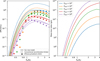 |
Fig. 1 Estimated efficiencies (left) and mass-loss rates (right) for fixed planetary mass Mp = 0.7 MJ but different EUV fluxes, from FEUV = 100erg/s/cm2 (red) to FEUV = 106 erg/s/cm2 (orange). The efficiency of the traditional recombination-limited approach is shown with dashed curves. In the intense EUV flux case, our model predictions are almost the same as the traditional approach (orange and purple). The fitted efficiencies from detailed 1D simulations by Caldiroli et al. (2021) are shown as points. Some points of the strong-gravity case (Mp > 20 MJ) cannot be seen in this panel due to the low efficiency. |
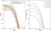 |
Fig. 2 Same as Fig. 1 but for a varying planetary mass (horizontal axis) and a fixed planetary radius, Rp = RJ . |
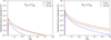 |
Fig. 3 Heating/cooling rate profiles for Mp = 0.7 MJ and Rp = 1.4 RJ with different physical conditions:Tch < Teq (left) and Tch > Teq (right). The solid curve shows the photoionization heating, and the dashed curves the radiative cooling and PdV cooling by gas expansion. |
3.2 Comparison to radiation hydrodynamic simulations
To validate the assumptions and outcomes of our analytic model, we performed our own 1D hydrodynamic simulations with EUV photoionization heating and Lyα radiative cooling, which dominate the heating and cooling processes in the upper atmosphere of typical hot Jupiters. We solved the following hydrodynamic equations:
 (15)
(15)
 (16)
(16)
 (17)
(17)
where ρ, υ, p, E, and H are the gas density, velocity, pressure, energy, and enthalpy per unit volume of gas. The effective gravitational potential Ψ can be given by  where ɑ, r* represents the semimajor axis and local distance to the host star as in Mitani et al. (2022). The simulations include photoionization heating and recombination cooling of hydrogen in Γ and Λ, respectively. EUV radiative transfer is handled using ray tracing. We implemented the Lyα cooling, which dominates the radiative cooling rate. We also solved for nonequilibrium chemistry:
 (18)
(18)
where yi = ni /nH and Ri represent the chemical abundance and the reaction rate, respectively. Our 1D hydrodynamic simulation code is based on the CIP method (Yabe & Aoki 1991). We initialized our simulations with a hydrostatic atmosphere and at the lower boundary, and we imposed a fixed surface temperature (1000 K) and density (n = 1014cm−3); the upper boundary allows the outflow to mimic the escaping atmosphere. The 1D simulations employ a spatial resolution of 5000 grid points, ensuring sufficient detail to resolve the ionization front and escape flow. We confirm that the 1D result is consistent with the open-source 1D code ATES (Caldiroli et al. 2021). We also confirm that the mass-loss rates of the 1D simulations are about four times higher than in 2D simulations, validating the assumption in Eq. (12) as discussed in previous studies (Murray-Clay et al. 2009).
Figure 3 shows the heating and cooling rate profiles for planets with Mp = 0.7 MJ and Rp = 1.4 RJ under different EUV fluxes (F0 = 1000,50000 erg/s/cm2). The higher flux is chosen so that the characteristic temperature exceeds the equilibrium temperature (Tch > Teq). In this case, we find that radiative cooling dominates the cooling process, and the system becomes recombination-limited. If the equilibrium temperature exceeds the characteristic temperature (Tch < Teq), the system becomes energy-limited. We also confirm that the gas temperature can be given by the gravitational temperature for low EUV and strong gravity planets. This condition is consistent with previous simulations by Murray-Clay et al. (2009).
The simulations confirm the outcome of the analytic model that the gas temperature is consistent with the gravitational temperature if Tch < Tg (the lower-flux model, F0 = 1000 erg cm−2s−1). We also ran 2D axisymmetric hydrodynamic simulations as in our previous study (Mitani et al. 2022) and confirm that the mass-loss rates of the 1D simulations are about four times higher than in 2D simulations, validating the assumption in Eq. (12) as discussed in previous studies (Murray-Clay et al. 2009).
4 Classification and understanding of observed exoplanets
Non-detections of Lyα, Hα, and helium triplet absorption have been found in some close-in exoplanets and the exact origin is still unknown: Stellar wind confinement and the absence of hydrogen-dominated atmospheres can both explain the nondetection of the escaping atmosphere. Based on the new analytic model, we can study the conditions in which non-detection can or cannot be explained by simple hydrogen-dominated atmospheric escape.
In this section we compare our analytic model in Sect. 3 to observed close-in exoplanets. We provide the method for finding peculiar exoplanets that may be affected by the stellar wind confinement, the absence of a hydrogen-dominated atmosphere, or other processes. We also provide the classification of observed exoplanets based on our essential parameters (Sect. 2) to reveal the underlying important physics in real systems.
4.1 Observational absorption signals
Recent observations have found some close-in planets with nondetections of hydrogen and helium absorption in their upper atmospheres. To demonstrate how our model can be applied to known close-in exoplanets with upper atmosphere observations, we used recent observational data from the MOPYS project (Orell-Miquel et al. 2024). In these data, planets are labeled with “Detection,” “Non Conclusive,” and “Non Detection” depending on whether hydrogen/helium were found.
Extreme-ultraviolet luminosity is difficult to observe in some systems. For many observed exoplanets in the data, we used X-rays and extreme-ultraviolet (XUV;1–912 Å) flux instead. For a few planets without XUV flux data, we estimated the XUV flux using the semimajor axis and the EUV luminosity of the star. We assumed the age-EUV luminosity relationships from Sanz-Forcada et al. (2011):
 (19)
(19)
where τ is the stellar age in gigayears. We also assumed that the EUV is monochromatic light with an energy of 20 eV to estimate the EUV photon flux, the cross section of photoionization, and the deposited energy from photoionization.
Our model depends on the average of the deposited energy, the cross section, and the photon number flux. The photoionization rate depends on F0σ0ΔE0 as in Eq. (3) and the base density also depends on the EUV flux.
We estimated the mass-loss rate of neutral hydrogen, ṀHI , assuming the timescale of photoionization and recombination at the base determines the neutral hydrogen mass-loss rate. The neutral hydrogen mass-loss rate is one of the factors that determine the Lyα transit depth (Owen et al. 2023). Lyα absorption is most likely detected in intermediate EUV environments, where vigorous winds are generated while retaining sufficient atomic hydrogen against photoionization. We note that the transit depth is linearly dependent on the gas sound speed and ionization rate and only logarithmically related to the overall mass loss rate (see Owen et al. 2023). The photoionization rate, sound speed, and the mass-loss rate of neutral hydrogen are not independent parameters. The Lyα transit depth in Owen (2023) can be a function of one of these three parameters. If we take into account the linear dependence of the photoionization rate, the trend in the prediction of observability is similar to the neutral mass-loss rate plot because the neutral hydrogen mass-loss rate tends to be lower in the case of a high photoionization rate, and the parameter associated with the photoionization rate is also smaller. The gas velocity also does not change the trend because the difference in the sound speed of the gas is usually within a factor of 2. Figure 4 shows the distribution of close-in planets with Lya observations on the map of Mp versus the estimated mass-loss rate of the neutral hydrogen. We applied the neutral hydrogen fraction at the base. Planets with detection do have high massloss rates of neutral hydrogen. The typical error in the mass-loss rates for planets (e.g., planets with ṀHI < 2 × 10¹⁰ g/s in Fig. 4) exposed to low EUV levels is a factor of 2. For planets with high EUV levels (planets with high mass-loss rate in Fig. 5), the error is a few tens of percent. However, the errors for highly irradiated planets might be somewhat underestimated since we uniformly adopted an equilibrium temperature of 104 K for these planets, neglecting variations that could arise from, for example, atmospheric metallicity. We discuss these effects in Sect. 5.2. The error in the equilibrium temperature can be a few tens of percent, which leads to an underestimation of the mass-loss rate error by a factor of 2.
The interstellar medium absorption prevents the observation of the Lyα line center and the radial acceleration due to the stellar wind or radiation pressure is necessary for the observed Lyman-alpha absorption in high-speed wings (McCann et al. 2019; Khodachenko et al. 2019; Schreyer et al. 2024). Since strong stellar winds are required to accelerate significant planetary outflows, our results suggest that planets with detected Lyα emissions have relatively strong stellar winds and high mass-loss rates. In contrast, planets with non-detections are expected to have stellar winds that are an order of magnitude weaker compared to those with detections, or they may experience extremely strong stellar winds that confine the planetary outflow (Mitani et al. 2022). Further modeling of the interaction between planetary outflows and stellar winds is necessary for understanding the non-detection of Lyα with a high mass-loss rate.
Through this analysis, we identified one outlier, K2-25 b, among the Lyα non-detection planets. This planet is located around the evaporation valley and may have lost its hydrogen-dominated atmosphere (Rockcliffe et al. 2021). As demonstrated here, our model has the potential to identify peculiar cases of non-detection/detection of the upper atmosphere’s absorption.
We also calculated the mass-loss rate of neutral hydrogen at the level n = 2 using the analytical formulae of level population Christie et al. (2013). The population of the 2p state is set by radiative excitation and deexcitation. The population of the 2s state is set by collisional excitation from the ground state and collisional deexcitation to the 2p state. The ratio of the population densities is given by

where A2p→1s and B1s→2p represent the Einstein coefficients for radiative transitions, JLyα is the radiative transition rate, and Ci→j denotes collisional transition rates from state i to state j. We calculated the population at the base to estimate the amount of launched excited hydrogen. It is important to note that the hydrogen population is inherently radially dependent throughout the escaping atmosphere. However, the absorption features observed in Hα transits are primarily dominated by hydrogen located near the planetary surface (Christie et al. 2013; Mitani et al. 2022). Consequently, we focused on the population at the base, under the assumption that the contribution from higher altitudes has a negligible impact on the overall absorption signal.
We assumed the stellar Lyα flux is proportional to the EUV flux. Figure 5 shows the distribution of planets with Hα observations. We find the clear separation around Mp ∼ 1030 g, which is consistent with the evaporation valley. Unlike Lyα observations, Hα absorption can be more significant in an intense EUV environment because Lyα radiation from the host star can excite neutral hydrogen, even though the neutral hydrogen fraction becomes lower in such environments. Among the Lyα nondetection planets, we find one outlier, WASP-77 b. This planet is a typical hot Jupiter with a metal-poor atmosphere (Smith et al. 2024), suggesting a high mass-loss rate due to reduced cooling (Sect. 5.2). Despite this, no evidence of Lyα absorption has been detected, which may indicate that the planet is significantly affected by stellar wind confinement.
Hα-detected planets have a large mass-loss rate of neutral hydrogen at the level n = 2. The population of n = 2 hydrogen depends on the stellar Lyα flux, which makes planets with intense EUV radiation easier to detect via Hα absorption, unlike Lyα absorption. According to our model, the non-detection of neutral hydrogen can be explained by a low mass-loss rate and is not necessarily due to stellar wind confinement or the absence of a hydrogen-dominated atmosphere in most cases. Our model can also be used to identify optimal targets for neutral hydrogen observations.
In summary, Lyα absorption is more likely to be detected in an intermediate EUV environment because low EUV radiation cannot drive a strong mass-loss outflow, while high EUV radiation photoionizes neutral hydrogen. Hα absorption, on the other hand, can be detected in a high EUV environment because strong Lyα emission excites neutral hydrogen.
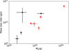 |
Fig. 4 Distribution of close-in planets with Lyα observations. The red (black) points represent the exoplanets in which hydrogen atoms have been (have not been) detected in Lyα. |
4.2 Classification of planetary outflow
To understand further physical conditions of observed exoplanets, we investigated relevant timescales and temperatures in observed exoplanets. We defined the ratio between the photoionization and recombination timescales from Eqs. (5) and (6) as
 (20)
(20)
The ratio equals unity when
 (21)
(21)
The condition tion = trec is represented by a straight line on the log(F0/Fcr)−log ξ plane in Fig. 6. Similarly, Teq = Tch draws another straight line. These lines divide the plane into at least three regions. Atmospheric escape is then classified into these regimes.
Figure 6 shows the distribution of planets with hydrogen observations on the log(F0/Fcr)−log ξ plane. Above the tion = trec line, photoionization reduces the neutral hydrogen not only in the tail but also in the launching atmosphere, making hydrogen observations difficult. This could explain why many planets have inconclusive detections, even though the flux from their stars seems high enough to initiate photoevaporation. It may be relatively easy to detect hydrogen in planets located below the tion = trec line, where the EUV flux exceeds the critical value. Such planets should be prioritized for future observations. The Tch = Teq line determines whether the radiative cooling dominates or not. In many close-in exoplanets with hydrogen observations, the intense radiation can heat the gas up to the equilibrium temperature.
Figure 7 shows the distribution of planets with helium absorption. While we do not observe a clear trend, it appears that planets with helium absorption are generally in high UV (Tch > Teq) environments. This correlation is expected, as high-UV conditions can lead to increased mass-loss rates and a higher fraction of helium in the triplet state. Helium absorption can be reduced by far-ultraviolet (FUV; <13.6 eV) radiation due to the ionization of excited 23S helium state (Oklopčić & Hirata 2018; Oklopčić 2019), which is not considered in this work. To consider the dependence on FUV flux, we categorized the planets based on their host star temperatures: hot (>5500 K) and cool (<5500 K). We find that most planets with non-detection of the helium absorption and experiencing high EUV flux have hot host stars, which likely possess higher FUV luminosities. In contrast, planets with detections and low EUV flux generally have cool host stars. This trend suggests that the EUV/FUV ratio can be a fundamental parameter of helium absorption. Further analytical investigation is required to better understand recent helium triplet observations.
It appears that classifying close-in planets based purely on the dimensionless parameters ξ and F0/Fcr does not reveal a trend in the detectability of hydrogen and helium escape. Instead, we need to look at the mass-loss rates of the observed species, considering their populations, as demonstrated in the previous section.
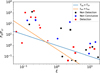 |
Fig. 6 Distribution of close-in exoplanets with hydrogen observations. The red points represent the exoplanets in which hydrogen has been detected in Lyα or Hα, the blue points planets with inconclusive detection in hydrogen absorption, and the black points planets in which hydrogen is not detected. Squares, circles, and stars represent planets with Lyα, Hα, and both line observations, respectively. The straight lines show the condition Teq = Tch and tion = trec. |
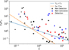 |
Fig. 7 Same as Fig. 6 but for exoplanets with helium observations. Circles and triangles represent planets with cool (<5500 K) and hot (>5500 K) host stars, respectively. |
5 Limitation of the model
5.1 Evolution of mass-loss regimes and planetary mass
The mass-loss timescale for sub-Neptunian planets plays a critical role in understanding the observational features of the sub-Neptunian valley. In the early stages (<1Gyr) of these planets, our model indicates a relatively low mass-loss efficiency (η < 0.1) due to significant cooling under strong radiation (FEUV > 105 erg/s/cm3). As the systems age to reduce the radiation strength, the efficiency approaches unity, leading to mass-loss rates that can exceed those predicted by traditional energy-limited assumptions. We note that the planetary radius decreases with time, and the mass-loss efficiency may also be affected. The planetary radius of high-mass planets decreases by approximately 10% over their lifetime (Fortney & Nettelmann 2010), and the effect is not significant. For low-mass planets, the radius changes by a factor of 2 over time, but the effect can be small because the efficiency is weakly dependent on the radius in low-gravity environments, as shown in Fig. 1. In total, the evolution of EUV luminosity dominates the evolution of the mass-loss rate. The mass loss during the early stage determines the total mass loss (e.g., Allan & Vidotto 2019). Consequently, the overall mass-loss timescale is extended, aligning qualitatively with the decreasing frequency of close-in exoplanets with ages (Berger et al. 2020).
In this study, we did not consider the impact of core-powered mass-loss. Recent theoretical models (Ginzburg et al. 2018; Owen & Schlichting 2024) propose that the core-powered massloss rate, Ṁcore , predominates when the Bondi radius is smaller than the effective planetary radius. Under such circumstances, we can assume that the gas velocity achieves sound speeds at the effective planetary radius. If  , where cinner is the sound speed in the inner atmosphere, the flow is driven by core-powered processes. Even if the EUV-driven mass-loss rate dominates the total mass loss, the core-powered flow can enhance the mass-loss flow as discussed in Owen & Schlichting (2024). In cases where core-powered processes are relevant, our model would require adjustments to account for changes in the base density derived from the core-powered mass loss model. Core-powered mass loss is particularly significant in low-mass and young planets. Near the radius gap, atmospheric escape driven by EUV photo-heating becomes crucial, especially as the efficiency increases in the later stages of planetary evolution.
5.2 X-ray and metal effects
In this study, we did not account for the heating effects of X-ray radiation and the cooling contributions of metal species. Recent observations have identified a hot Jupiter with a metalrich upper atmosphere, which current classical mass-loss models fail to explain adequately. In such environments, X-rays can significantly elevate gas temperatures and penetrate deeper layers owing to their small cross sections. For metal-poor gases, the density required to initiate atmospheric launching can be substantially higher, as it inversely correlates with the cross section; consequently, the characteristic temperature for X-ray photoheating might be notably low. X-ray heating becomes negligible when the energy deposit of X-ray flux is smaller than that of EUV flux. Typically, the mass-loss rates driven by X-rays are lower than those driven by EUV radiation in many planetary atmospheres.
Even when incorporating the effects of metal coolants, our model is readily available once the equilibrium temperature is modified accordingly. In cases where metals like Fe and Mg are present, metal line cooling could predominate the cooling mechanisms due to their higher abundances. For instance, the cooling rates for Mg and O are more substantial compared to other metals.
We calculated the Mg II cooling, which can be dominant in close-in planetary atmosphere (Huang et al. 2023). For real planets, many metal species contribute to the cooling rate. It is difficult to understand the physics of atmospheric escape with many metal coolants. We focused on what happens in atmosphere with one dominant metal species to investigate the physics of metal-rich atmosphere. The Mg II cooling rate is
 (22)
(22)
where fMg is the fraction of Mg II, we used the value of excitation energy, ΔE, the radiative decay rate, Aul, and the critical density, ncrit, from Huang et al. (2017). The equilibrium temperature was calculated by solving
 (23)
(23)
We calculated the characteristic temperature and the photoheating and cooling rates at the base using fixed planetary parameters (Mp = 0.7 MJ and Rp = 1010 cm) and varying EUV flux. We defined the characteristic temperature as the metallicity-dependent equilibrium temperature when Eq. (23) is satisfied.
Figure 8 shows the metallicity dependence of the equilibrium temperature. We find that the equilibrium temperature is ~5000 K in metal-rich (Z > 10 Z⊙) planets due to the strong cooling by Mg II and the mass-loss rate of such a metalrich planet can be significantly lower than the rate of subsolar metallicity planets.
The Lyα cooling rate is influenced by the electron density, as Lyα radiation results from hydrogen atoms being collisionally excited by electrons. Therefore, the abundance of elements like Fe, which contribute to the electron density through ionization, is also significant. However, despite these metal effects, the Lya cooling rate predominantly depends on the gas temperature, maintaining the equilibrium temperature at approximately 104 K in subsolar metallicity planets.
Observationally, the presence of metals complicates the scenario further. Metals increase the electron density through ionization, which in turn shortens the recombination timescale. This effect can be important in planets around massive stars with low EUV luminosity. The effect could enhance the observational transit depth in measurements of hydrogen neutral atoms, even though the metal cooling itself tends to reduce the hydrogen mass-loss rate.
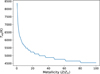 |
Fig. 8 Metallicity dependence of the equilibrium temperature. |
6 Conclusions
Extreme-ultraviolet-driven atmospheric escape is a key process in the evolution of close-in exoplanets. In many previous planetary evolution studies, a constant mass-loss efficiency was assumed despite radiation hydrodynamic simulations revealing that the efficiency depends on the stellar and planetary parameters. Deriving analytical formulae for the mass-loss is crucial for understanding the exoplanetary evolution.
We introduced essential parameters to describe photoheating, gas expansion, and gravitational effects within planetary atmospheres. The temperature dynamics are characterized by three distinct measures: the characteristic temperature, the equilibrium temperature, and the gravitational temperature. The characteristic temperature quantifies the intensity of photo-heating and is defined as a function of the photo-heating rate. The equilibrium temperature results from the balance between photoheating and radiative cooling, while the gravitational temperature reflects the influence of planetary gravity on the atmospheric structure.
Based on these quantities, we developed an analytical model for EUV-driven atmospheric escape in a hydrogen-dominated atmosphere. Our analytical model is capable of predicting the mass-loss efficiency across a broad spectrum of stellar and planetary parameters, bridging the gap between the energylimited (low-EUV-flux) and recombination-limited (high-EUV-flux) regimes.
Our model indicates that the efficiency is greater than 10% for many energy-limited and low-gravity planets and that planets exhibiting Lyα absorption generally have significant mass-loss rates of neutral hydrogen, exceeding 1010 g/s. These planets typically experience an intermediate range of EUV flux; insufficient EUV flux fails to drive substantial outflows, whereas intense EUV flux leads to extensive photoionization of neutral hydrogen. Furthermore, we observe a correlation between the mass-loss rate of neutral hydrogen in the excited state (n = 2) and the Hα absorption signature. Planets showing Hα absorption are typically subjected to strong EUV flux and exhibit high mass-loss rates of excited hydrogen, often exceeding 103 g/s.
Our model also identifies peculiar cases of exoplanets whose upper atmosphere observations deviate from predictions by classical EUV-driven models of hydrogen-dominated atmospheres. Such outliers may have depleted their hydrogen-dominated atmospheres, or their upper atmospheres could be confined by strong stellar winds, reducing their absorption signatures.
In the future, our model can be adapted to include atmospheres with metal line cooling and other photo-heating processes. These intricate physical phenomena could generalize the equilibrium/characteristic temperatures and thereby the overall mass-loss efficiency of exoplanets.
Acknowledgements
HM has been supported by International Graduate Program for Excellence in Earth-Space Science (IGPEES) of the University of Tokyo and JSPS Overseas Research Fellowship. RK acknowledges financial support via the Heisenberg Research Grant funded by the Deutsche Forschungsgemeinschaft (DFG, German Research Foundation) under grant no. KU 2849/9, project no. 445783058. RK also acknowledges financial support from the JSPS Invitational Fellowship for Research in Japan under the Fellowship ID S20156. We thank Naoki Yoshida for the fruitful discussions. Numerical computations were in part carried out on the Cray XC50 at the Center for Computational Astrophysics, National Astronomical Observatory of Japan.
References
- Allan, A., & Vidotto, A. A. 2019, MNRAS, 490, 3760 [Google Scholar]
- Allart, R., Lemée-Joliecoeur, P. B., Jaziri, A. Y., et al. 2023, A&A, 677, A164 [NASA ADS] [CrossRef] [EDP Sciences] [Google Scholar]
- Begelman, M. C., McKee, C. F., & Shields, G. A. 1983, ApJ, 271, 70 [CrossRef] [Google Scholar]
- Bennett, K. A., Redfield, S., Oklopčić, A., et al. 2023, AJ, 165, 264 [NASA ADS] [CrossRef] [Google Scholar]
- Berger, T. A., Huber, D., Gaidos, E., van Saders, J. L., & Weiss, L. M. 2020, AJ, 160, 108 [NASA ADS] [CrossRef] [Google Scholar]
- Caldiroli, A., Haardt, F., Gallo, E., et al. 2021, A&A, 655, A30 [NASA ADS] [CrossRef] [EDP Sciences] [Google Scholar]
- Carolan, S., Vidotto, A. A., Plavchan, P., Villarreal D’Angelo, C., & Hazra, G. 2020, MNRAS, 498, L53 [NASA ADS] [CrossRef] [Google Scholar]
- Cauley, P. W., Redfield, S., & Jensen, A. G. 2017, AJ, 153, 217 [NASA ADS] [CrossRef] [Google Scholar]
- Christie, D., Arras, P., & Li, Z.-Y. 2013, ApJ, 772, 144 [NASA ADS] [CrossRef] [Google Scholar]
- Ehrenreich, D., Bourrier, V., Wheatley, P. J., et al. 2015, Nature, 522, 459 [Google Scholar]
- Erkaev, N. V., Kulikov, Y. N., Lammer, H., et al. 2007, A&A, 472, 329 [NASA ADS] [CrossRef] [EDP Sciences] [Google Scholar]
- Fortney, J. J., & Nettelmann, N. 2010, Space Sci. Rev., 152, 423 [CrossRef] [Google Scholar]
- Fujita, N., Hori, Y., & Sasaki, T. 2022, ApJ, 928, 105 [NASA ADS] [CrossRef] [Google Scholar]
- Fulton, B. J., Petigura, E. A., Howard, A. W., et al. 2017, AJ, 154, 109 [Google Scholar]
- Ginzburg, S., Schlichting, H. E., & Sari, R. 2018, MNRAS, 476, 759 [Google Scholar]
- Gupta, A., & Schlichting, H. E. 2019, MNRAS, 487, 24 [Google Scholar]
- Huang, C., Arras, P., Christie, D., & Li, Z.-Y. 2017, ApJ, 851, 150 [NASA ADS] [CrossRef] [Google Scholar]
- Huang, C., Koskinen, T., Lavvas, P., & Fossati, L. 2023, ApJ, 951, 123 [NASA ADS] [CrossRef] [Google Scholar]
- Khodachenko, M. L., Shaikhislamov, I. F., Lammer, H., et al. 2019, ApJ, 885, 67 [NASA ADS] [CrossRef] [Google Scholar]
- Kubyshkina, D., Fossati, L., Erkaev, N. V., et al. 2018a, ApJ, 866, L18 [NASA ADS] [CrossRef] [Google Scholar]
- Kubyshkina, D., Fossati, L., Erkaev, N. V., et al. 2018b, A&A, 619, A151 [NASA ADS] [CrossRef] [EDP Sciences] [Google Scholar]
- Kulow, J. R., France, K., Linsky, J., & Loyd, R. O. P. 2014, ApJ, 786, 132 [Google Scholar]
- Kurokawa, H., & Nakamoto, T. 2014, ApJ, 783, 54 [NASA ADS] [CrossRef] [Google Scholar]
- Lammer, H., Selsis, F., Ribas, I., et al. 2003, ApJ, 598, L121 [Google Scholar]
- Lecavelier Des Etangs, A., Ehrenreich, D., Vidal-Madjar, A., et al. 2010, A&A, 514, A72 [NASA ADS] [CrossRef] [EDP Sciences] [Google Scholar]
- Lopez, E. D., & Fortney, J. J. 2013, ApJ, 776, 2 [Google Scholar]
- Mazeh, T., Holczer, T., & Faigler, S. 2016, A&A, 589, A75 [NASA ADS] [CrossRef] [EDP Sciences] [Google Scholar]
- McCann, J., Murray-Clay, R. A., Kratter, K., & Krumholz, M. R. 2019, ApJ, 873, 89 [NASA ADS] [CrossRef] [Google Scholar]
- Mitani, H., Nakatani, R., & Yoshida, N. 2022, MNRAS, 512, 855 [NASA ADS] [CrossRef] [Google Scholar]
- Murray-Clay, R. A., Chiang, E. I., & Murray, N. 2009, ApJ, 693, 23 [Google Scholar]
- Nakatani, R., Turner, N. J., & Takasao, S. 2024, arXiv e-prints [arXiv:2406.18461] [Google Scholar]
- Oklopčić, A. 2019, ApJ, 881, 133 [Google Scholar]
- Oklopčić, A., & Hirata, C. M. 2018, ApJ, 855, L11 [Google Scholar]
- Orell-Miquel, J., Murgas, F., Pallé, E., et al. 2024, A&A, 689, A179 [NASA ADS] [CrossRef] [EDP Sciences] [Google Scholar]
- Owen, J. E. 2019, Annu. Rev. Earth Planet. Sci., 47, 67 [CrossRef] [Google Scholar]
- Owen, J. E., & Alvarez, M. A. 2016, ApJ, 816, 34 [Google Scholar]
- Owen, J. E., & Jackson, A. P. 2012, MNRAS, 425, 2931 [Google Scholar]
- Owen, J. E., & Wu, Y. 2017, ApJ, 847, 29 [Google Scholar]
- Owen, J. E., & Schlichting, H. E. 2024, MNRAS, 528, 1615 [NASA ADS] [CrossRef] [Google Scholar]
- Owen, J. E., Murray-Clay, R. A., Schreyer, E., et al. 2023, MNRAS, 518, 4357 [Google Scholar]
- Rockcliffe, K. E., Newton, E. R., Youngblood, A., et al. 2021, AJ, 162, 116 [NASA ADS] [CrossRef] [Google Scholar]
- Sanz-Forcada, J., Micela, G., Ribas, I., et al. 2011, A&A, 532, A6 [NASA ADS] [CrossRef] [EDP Sciences] [Google Scholar]
- Schreyer, E., Owen, J. E., Loyd, R. O. P., & Murray-Clay, R. 2024, MNRAS, 533, 3296 [Google Scholar]
- Smith, P. C. B., Line, M. R., Bean, J. L., et al. 2024, AJ, 167, 110 [NASA ADS] [CrossRef] [Google Scholar]
- Spake, J. J., Sing, D. K., Evans, T. M., et al. 2018, Nature, 557, 68 [Google Scholar]
- Vidal-Madjar, A., Lecavelier des Etangs, A., Désert, J. M., et al. 2003, Nature, 422, 143 [Google Scholar]
- Watson, A. J., Donahue, T. M., & Walker, J. C. G. 1981, Icarus, 48, 150 [NASA ADS] [CrossRef] [Google Scholar]
- Woods, D. T., Klein, R. I., Castor, J. I., McKee, C. F., & Bell, J. B. 1996, ApJ, 461, 767 [NASA ADS] [CrossRef] [Google Scholar]
- Yabe, T., & Aoki, T. 1991, Comput. Phys. Commun., 66, 219 [Google Scholar]
- Yan, F., Wyttenbach, A., Casasayas-Barris, N., et al. 2021, A&A, 645, A22 [EDP Sciences] [Google Scholar]
- Yelle, R. V. 2004, Icarus, 170, 167 [NASA ADS] [CrossRef] [Google Scholar]
- Zhang, M., Knutson, H. A., Wang, L., Dai, F., & Barragán, O. 2022, AJ, 163, 67 [NASA ADS] [CrossRef] [Google Scholar]
All Tables
All Figures
|
Fig. 1 Estimated efficiencies (left) and mass-loss rates (right) for fixed planetary mass Mp = 0.7 MJ but different EUV fluxes, from FEUV = 100erg/s/cm2 (red) to FEUV = 106 erg/s/cm2 (orange). The efficiency of the traditional recombination-limited approach is shown with dashed curves. In the intense EUV flux case, our model predictions are almost the same as the traditional approach (orange and purple). The fitted efficiencies from detailed 1D simulations by Caldiroli et al. (2021) are shown as points. Some points of the strong-gravity case (Mp > 20 MJ) cannot be seen in this panel due to the low efficiency. |
| In the text | |
|
Fig. 2 Same as Fig. 1 but for a varying planetary mass (horizontal axis) and a fixed planetary radius, Rp = RJ . |
| In the text | |
|
Fig. 3 Heating/cooling rate profiles for Mp = 0.7 MJ and Rp = 1.4 RJ with different physical conditions:Tch < Teq (left) and Tch > Teq (right). The solid curve shows the photoionization heating, and the dashed curves the radiative cooling and PdV cooling by gas expansion. |
| In the text | |
|
Fig. 4 Distribution of close-in planets with Lyα observations. The red (black) points represent the exoplanets in which hydrogen atoms have been (have not been) detected in Lyα. |
| In the text | |
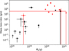 |
Fig. 5 Same as Fig. 4 but for planets with Hα observations. |
| In the text | |
|
Fig. 6 Distribution of close-in exoplanets with hydrogen observations. The red points represent the exoplanets in which hydrogen has been detected in Lyα or Hα, the blue points planets with inconclusive detection in hydrogen absorption, and the black points planets in which hydrogen is not detected. Squares, circles, and stars represent planets with Lyα, Hα, and both line observations, respectively. The straight lines show the condition Teq = Tch and tion = trec. |
| In the text | |
|
Fig. 7 Same as Fig. 6 but for exoplanets with helium observations. Circles and triangles represent planets with cool (<5500 K) and hot (>5500 K) host stars, respectively. |
| In the text | |
|
Fig. 8 Metallicity dependence of the equilibrium temperature. |
| In the text | |
Current usage metrics show cumulative count of Article Views (full-text article views including HTML views, PDF and ePub downloads, according to the available data) and Abstracts Views on Vision4Press platform.
Data correspond to usage on the plateform after 2015. The current usage metrics is available 48-96 hours after online publication and is updated daily on week days.
Initial download of the metrics may take a while.