| Issue |
A&A
Volume 694, February 2025
|
|
|---|---|---|
| Article Number | A321 | |
| Number of page(s) | 22 | |
| Section | Cosmology (including clusters of galaxies) | |
| DOI | https://doi.org/10.1051/0004-6361/202452531 | |
| Published online | 24 February 2025 | |
Euclid: Relativistic effects in the dipole of the two-point correlation function⋆
1
Department of Astrophysics, University of Zurich, Winterthurerstrasse 190, 8057 Zurich, Switzerland
2
Institut de Recherche en Astrophysique et Planétologie (IRAP), Université de Toulouse, CNRS, UPS, CNES, 14 Av. Edouard Belin, 31400 Toulouse, France
3
Institute of Space Sciences (ICE, CSIC), Campus UAB, Carrer de Can Magrans, s/n, 08193 Barcelona, Spain
4
Institut de Ciencies de l’Espai (IEEC-CSIC), Campus UAB, Carrer de Can Magrans, s/n Cerdanyola del Vallés, 08193 Barcelona, Spain
5
Laboratoire Univers et Théorie, Observatoire de Paris, Université PSL, Université Paris Cité, CNRS, 92190 Meudon, France
6
Kobayashi-Maskawa Institute for the Origin of Particles and the Universe, Nagoya University, Chikusa-ku, Nagoya 464-8602, Japan
7
Institute for Advanced Research, Nagoya University, Chikusa-ku, Nagoya 464-8601, Japan
8
Institut d’Estudis Espacials de Catalunya (IEEC), Edifici RDIT, Campus UPC, 08860 Castelldefels, Barcelona, Spain
9
Université de Genève, Département de Physique Théorique and Centre for Astroparticle Physics, 24 quai Ernest-Ansermet, CH-1211 Genève 4, Switzerland
10
Institut für Theoretische Physik, University of Heidelberg, Philosophenweg 16, 69120 Heidelberg, Germany
11
INAF-Osservatorio Astronomico di Brera, Via Brera 28, 20122 Milano, Italy
12
IFPU, Institute for Fundamental Physics of the Universe, via Beirut 2, 34151 Trieste, Italy
13
INAF-Osservatorio Astronomico di Trieste, Via G. B. Tiepolo 11, 34143 Trieste, Italy
14
INFN, Sezione di Trieste, Via Valerio 2, 34127 Trieste, TS, Italy
15
SISSA, International School for Advanced Studies, Via Bonomea 265, 34136 Trieste, TS, Italy
16
Dipartimento di Fisica e Astronomia, Università di Bologna, Via Gobetti 93/2, 40129 Bologna, Italy
17
INAF-Osservatorio di Astrofisica e Scienza dello Spazio di Bologna, Via Piero Gobetti 93/3, 40129 Bologna, Italy
18
INFN-Sezione di Bologna, Viale Berti Pichat 6/2, 40127 Bologna, Italy
19
INAF-Osservatorio Astrofisico di Torino, Via Osservatorio 20, 10025 Pino Torinese, (TO), Italy
20
Dipartimento di Fisica, Università di Genova, Via Dodecaneso 33, 16146 Genova, Italy
21
INFN-Sezione di Genova, Via Dodecaneso 33, 16146, Genova, Italy
22
Department of Physics “E. Pancini”, University Federico II, Via Cinthia 6, 80126 Napoli, Italy
23
INAF-Osservatorio Astronomico di Capodimonte, Via Moiariello 16, 80131 Napoli, Italy
24
INFN section of Naples, Via Cinthia 6, 80126 Napoli, Italy
25
Instituto de Astrofísica e Ciências do Espaço, Universidade do Porto, CAUP, Rua das Estrelas, PT4150-762 Porto, Portugal
26
Faculdade de Ciências da Universidade do Porto, Rua do Campo de Alegre, 4150-007 Porto, Portugal
27
Aix-Marseille Université, CNRS, CNES, LAM, Marseille, France
28
Dipartimento di Fisica, Università degli Studi di Torino, Via P. Giuria 1, 10125 Torino, Italy
29
INFN-Sezione di Torino, Via P. Giuria 1, 10125 Torino, Italy
30
INAF-IASF Milano, Via Alfonso Corti 12, 20133 Milano, Italy
31
Centro de Investigaciones Energéticas, Medioambientales y Tecnológicas (CIEMAT), Avenida Complutense 40, 28040 Madrid, Spain
32
Port d’Informació Científica, Campus UAB, C. Albareda s/n, 08193 Bellaterra (Barcelona), Spain
33
Institute for Theoretical Particle Physics and Cosmology (TTK), RWTH Aachen University, 52056 Aachen, Germany
34
Institute of Cosmology and Gravitation, University of Portsmouth, Portsmouth PO1 3FX, UK
35
INAF-Osservatorio Astronomico di Roma, Via Frascati 33, 00078 Monteporzio Catone, Italy
36
Dipartimento di Fisica e Astronomia “Augusto Righi” – Alma Mater Studiorum Università di Bologna, Viale Berti Pichat 6/2, 40127 Bologna, Italy
37
Instituto de Astrofísica de Canarias, Calle Vía Láctea s/n, 38204 San Cristóbal de La Laguna, Tenerife, Spain
38
Institute for Astronomy, University of Edinburgh, Royal Observatory, Blackford Hill, Edinburgh EH9 3HJ, UK
39
European Space Agency/ESRIN, Largo Galileo Galilei 1, 00044 Frascati, Roma, Italy
40
ESAC/ESA, Camino Bajo del Castillo, s/n., Urb. Villafranca del Castillo, 28692 Villanueva de la Cañada, Madrid, Spain
41
Université Claude Bernard Lyon 1, CNRS/IN2P3, IP2I Lyon, UMR 5822, Villeurbanne F-69100, France
42
Institut de Ciències del Cosmos (ICCUB), Universitat de Barcelona (IEEC-UB), Martí i Franquès 1, 08028 Barcelona, Spain
43
Institució Catalana de Recerca i Estudis Avançats (ICREA), Passeig de Lluís Companys 23, 08010 Barcelona, Spain
44
UCB Lyon 1, CNRS/IN2P3, IUF, IP2I Lyon, 4 rue Enrico Fermi, 69622 Villeurbanne, France
45
Department of Astronomy, University of Geneva, ch. d’Ecogia 16, 1290 Versoix, Switzerland
46
Jodrell Bank Centre for Astrophysics, Department of Physics and Astronomy, University of Manchester, Oxford Road, Manchester M13 9PL, UK
47
INFN-Padova, Via Marzolo 8, 35131 Padova, Italy
48
INAF-Istituto di Astrofisica e Planetologia Spaziali, via del Fosso del Cavaliere, 100, 00100 Roma, Italy
49
Université Paris-Saclay, Université Paris Cité, CEA, CNRS, AIM, 91191 Gif-sur-Yvette, France
50
INAF-Osservatorio Astronomico di Padova, Via dell’Osservatorio 5, 35122 Padova, Italy
51
Max Planck Institute for Extraterrestrial Physics, Giessenbachstr. 1, 85748 Garching, Germany
52
Universitäts-Sternwarte München, Fakultät für Physik, Ludwig-Maximilians-Universität München, Scheinerstrasse 1, 81679 München, Germany
53
Institute of Theoretical Astrophysics, University of Oslo, P.O. Box 1029 Blindern, 0315 Oslo, Norway
54
Jet Propulsion Laboratory, California Institute of Technology, 4800 Oak Grove Drive, Pasadena, CA 91109, USA
55
Felix Hormuth Engineering, Goethestr. 17, 69181 Leimen, Germany
56
Technical University of Denmark, Elektrovej 327, 2800 Kgs., Lyngby, Denmark
57
Cosmic Dawn Center (DAWN), Copenhagen, Denmark
58
Université Paris-Saclay, CNRS/IN2P3, IJCLab, 91405 Orsay, France
59
Max-Planck-Institut für Astronomie, Königstuhl 17, 69117 Heidelberg, Germany
60
NASA Goddard Space Flight Center, Greenbelt, MD 20771, USA
61
Department of Physics and Helsinki Institute of Physics, Gustaf Hällströmin katu 2, 00014 University of Helsinki, Finland
62
Department of Physics, P.O. Box 64 00014 University of Helsinki, Finland
63
Helsinki Institute of Physics, Gustaf Hällströmin katu 2, University of Helsinki, Helsinki, Finland
64
NOVA optical infrared instrumentation group at ASTRON, Oude Hoogeveensedijk 4, 7991 PD Dwingeloo, The Netherlands
65
Universität Bonn, Argelander-Institut für Astronomie, Auf dem Hügel 71, 53121 Bonn, Germany
66
INFN-Sezione di Roma, Piazzale Aldo Moro, 2 – c/o Dipartimento di Fisica, Edificio G. Marconi, 00185 Roma, Italy
67
Dipartimento di Fisica e Astronomia “Augusto Righi” – Alma Mater Studiorum Università di Bologna, via Piero Gobetti 93/2, 40129 Bologna, Italy
68
Department of Physics, Institute for Computational Cosmology, Durham University, South Road DH1 3LE, UK
69
University of Applied Sciences and Arts of Northwestern Switzerland, School of Engineering, 5210 Windisch, Switzerland
70
Institut d’Astrophysique de Paris, 98bis Boulevard Arago, 75014 Paris, France
71
Institut d’Astrophysique de Paris, UMR 7095, CNRS, and Sorbonne Université, 98 bis boulevard Arago, 75014 Paris, France
72
Institute of Physics, Laboratory of Astrophysics, Ecole Polytechnique Fédérale de Lausanne (EPFL), Observatoire de Sauverny, 1290 Versoix, Switzerland
73
Institut de Física d’Altes Energies (IFAE), The Barcelona Institute of Science and Technology, Campus UAB, 08193 Bellaterra (Barcelona), Spain
74
European Space Agency/ESTEC, Keplerlaan 1, 2201 AZ Noordwijk, The Netherlands
75
DARK, Niels Bohr Institute, University of Copenhagen, Jagtvej 155, 2200 Copenhagen, Denmark
76
Space Science Data Center, Italian Space Agency, via del Politecnico snc, 00133 Roma, Italy
77
Centre National d’Etudes Spatiales – Centre spatial de Toulouse, 18 avenue Edouard Belin, 31401 Toulouse Cedex 9, France
78
Institute of Space Science, Str. Atomistilor, nr. 409 Măgurele, Ilfov 077125, Romania
79
Dipartimento di Fisica e Astronomia “G. Galilei”, Università di Padova, Via Marzolo 8, 35131 Padova, Italy
80
Université Paris Cité, CNRS, Astroparticule et Cosmologie, 75013 Paris, France
81
Université St Joseph; Faculty of Sciences, Beirut, Lebanon
82
Departamento de Física, FCFM, Universidad de Chile, Blanco Encalada, 2008 Santiago, Chile
83
Universität Innsbruck, Institut für Astro- und Teilchenphysik, Technikerstr. 25/8, 6020 Innsbruck, Austria
84
Aix-Marseille Université, CNRS/IN2P3, CPPM, Marseille, France
85
Satlantis, University Science Park, Sede Bld, 48940 Leioa-Bilbao, Spain
86
Departamento de Física, Faculdade de Ciências, Universidade de Lisboa, Edifício C8, Campo Grande, PT1749-016 Lisboa, Portugal
87
Instituto de Astrofísica e Ciências do Espaço, Faculdade de Ciências, Universidade de Lisboa, Tapada da Ajuda, 1349-018 Lisboa, Portugal
88
Universidad Politécnica de Cartagena, Departamento de Electrónica y Tecnología de Computadoras, Plaza del Hospital 1, 30202 Cartagena, Spain
89
INFN-Bologna, Via Irnerio 46, 40126 Bologna, Italy
90
Infrared Processing and Analysis Center, California Institute of Technology, Pasadena, CA 91125, USA
91
INAF, Istituto di Radioastronomia, Via Piero Gobetti 101, 40129 Bologna, Italy
92
Kavli Institute for Cosmology Cambridge, Madingley Road, Cambridge CB3 0HA, UK
93
Institute of Astronomy, University of Cambridge, Madingley Road, Cambridge CB3 0HA, UK
94
Junia, EPA department, 41 Bd Vauban, 59800 Lille, France
95
ICSC – Centro Nazionale di Ricerca in High Performance Computing, Big Data e Quantum Computing, Via Magnanelli 2, Bologna, Italy
⋆⋆ Corresponding author; This email address is being protected from spambots. You need JavaScript enabled to view it.
Received:
8
October
2024
Accepted:
20
December
2024
Abstract
Gravitational redshift and Doppler effects give rise to an antisymmetric component of the galaxy correlation function when cross-correlating two galaxy populations or two different tracers. In this paper, we assess the detectability of these effects in the Euclid spectroscopic galaxy survey. We model the impact of gravitational redshift on the observed redshift of galaxies in the Flagship mock catalogue using a Navarro–Frenk–White profile for the host haloes. We isolate these relativistic effects, largely subdominant in the standard analysis, by splitting the galaxy catalogue into two populations of faint and bright objects and estimating the dipole of their cross-correlation in four redshift bins. In the simulated catalogue, we detect the dipole signal on scales below 30 h−1 Mpc, with detection significances of 4σ and 3σ in the two lowest redshift bins, respectively. At higher redshifts, the detection significance drops below 2σ. Overall, we estimate the total detection significance in the Euclid spectroscopic sample to be approximately 6σ. We find that on small scales, the major contribution to the signal comes from the nonlinear gravitational potential. Our study on the Flagship mock catalogue shows that this observable can be detected in Euclid Data Release 2 and beyond.
Key words: cosmology: theory / large-scale structure of Universe
This paper is published on behalf of the Euclid Consortium.
© The Authors 2025
 Open Access article, published by EDP Sciences, under the terms of the Creative Commons Attribution License (https://creativecommons.org/licenses/by/4.0), which permits unrestricted use, distribution, and reproduction in any medium, provided the original work is properly cited.
This article is published in open access under the Subscribe to Open model. This email address is being protected from spambots. You need JavaScript enabled to view it. to support open access publication.
1. Introduction
The current picture of the Universe and its evolution history is based on the concordance Λ cold dark matter (ΛCDM) model, which describes gravitational phenomena according to the laws of general relativity and assumes the Universe to be statistically homogeneous and isotropic on cosmological scales. This simple model is capable of fitting a wide variety of observations: the temperature and polarisation anisotropies of the cosmic microwave background (Hinshaw et al. 2013; Planck Collaboration I 2020), the clustering of galaxies on large scales (Alam et al. 2021; DESI Collaboration 2024), weak gravitational lensing, which causes distortion in the observed shapes of galaxies (Abbott et al. 2022), and the distance measurements from supernovae (Scolnic et al. 2018; DES Collaboration 2024). However, the standard model is not fully satisfactory. From a theoretical point of view, it requires that the majority of the energy content in our Universe takes some unknown form: a cosmological constant, whose inferred value lacks fundamental understanding, drives the current accelerated expansion of the Universe, while the matter content is mostly composed of a non-baryonic component that is yet to be directly detected. Furthermore, as recent cosmological experiments have become more precise, some tensions between parameters inferred from different probes have emerged (Di Valentino et al. 2021a,b; Schöneberg et al. 2022; DESI Collaboration 2024; Tutusaus et al. 2023a). Currently, it remains unclear whether these discrepancies either reveal a breakdown of the ΛCDM model, a sign that astrophysical or systematic effects have been overlooked in the analyses in tension, or whether they are nothing more than a statistical fluke.
One of the main goals of the next generation of cosmological surveys is to resolve these issues, in particular by testing one of the pillars of the standard model: Einstein’s theory of general relativity. In the near future, the Euclid Survey (Laureijs et al. 2011; Amendola et al. 2018; Euclid Collaboration: Mellier et al. 2025) is set to play a key role in this challenge. By using two complementary probes – weak lensing (including galaxy clustering and galaxy-galaxy lensing from its photometric survey) and 3D galaxy clustering (from its spectroscopic survey) – Euclid will map the expansion history of the Universe as well as the growth of cosmic structure within it.
The Euclid Spectroscopic Survey will provide a catalogue of more than 25 million emission-line galaxies using slitless spectroscopy for redshift determination, in the redshift range between z = 0.9 and z = 1.8. One of the key measurements that Euclid will carry out from these data is that of the growth rate at different cosmic times, using redshift-space distortions (RSDs; Kaiser 1987). RSDs manifest because we do not directly observe galaxies where they are but rather infer their physical distances from their observed redshifts, assuming that the latter is approximately given by the Hubble expansion. However, the observed redshift is also affected by the peculiar velocities of galaxies through the Doppler shift, for example. Since we do not know the peculiar velocities of individual objects, we cannot correct each redshift individually but rather model the distortions induced by the peculiar motions in the two-point statistics. The main effect is that galaxies moving along the line-of-sight toward an overdensity will appear closer to each other. Therefore, the observed two-point correlation function (or its Fourier counterpart, the power spectrum) is not isotropic, but also includes even multipoles (quadrupole and hexadecapole) that can be measured to extract cosmological information (Alam et al. 2016; Sanchez et al. 2017).
More recently, a fully relativistic computation has shown that in addition to the Kaiser RSDs, typically exploited in anisotropic galaxy clustering analysis, there are other subtle physical effects that can also influence the observed distribution of galaxies, such as gravitational redshift, Doppler effects, Shapiro time delay, and the integrated Sachs–Wolfe effect (Yoo et al. 2009; Yoo 2010; Bonvin & Durrer 2011; Challinor & Lewis 2011; Jeong et al. 2012). Although their impact on even multipoles of the correlation function has been shown to be negligible even for future galaxy surveys (Jelic-Cizmek et al. 2021), it is possible to isolate them using multiple tracers. Importantly, while standard RSDs generate only even multipoles of the correlation function at leading order, the gravitational redshift and further Doppler-type contributions generate odd multipoles in the two-point cross-correlation function (McDonald 2009; Bonvin et al. 2014).
Measuring the odd multipoles is interesting, as they provide complementary information to the even multipoles. In particular, the dipole is sourced in part by the gravitational redshift, so in principle is sensitive to the distortion of time (Sobral-Blanco & Bonvin 2022). Measuring the distortion of time through the dipole, in combination with existing probes, would thus allow for a range of novel tests. These include: a test of the validity of the equivalence principle for dark matter, by combining with RSDs (Bonvin & Fleury 2018), a test of the validity of local position invariance (Saga et al. 2023), a novel way to measure the anisotropic stress, by combining with weak gravitational lensing (Sobral-Blanco & Bonvin 2021; Tutusaus et al. 2023b), and more generally a way to distinguish between modifications of gravity and additional forces in the dark sector (Castello et al. 2022; Bonvin & Pogosian 2023; Castello et al. 2024). Furthermore, the dipole and octupole can be used to improve our understanding of astrophysical properties of galaxies (Sobral-Blanco et al. 2024).
Gravitational redshift has been measured in galaxy clusters (Wojtak et al. 2011; Sadeh et al. 2015; Rosselli et al. 2023), and also in large-scale structure, with a 2.8σ detection of the relativistic dipole reported at scales below 10 h−1 Mpc using data from SDSS-III (Alam et al. 2017). The detectability of the dipole has been investigated for different combinations of tracers and future cosmological surveys using analytical models for both signals and covariance, showing that it will be robustly detected in the linear and nonlinear regime, see for example Bonvin et al. (2016), Hall & Bonvin (2017), Lepori et al. (2018), Bonvin & Fleury (2018), Lepori et al. (2020) and Saga et al. (2022). The dipole has moreover been detected in N-body simulations, cross-correlating halo populations with different masses (Breton et al. 2019; Beutler & Di Dio 2020), and galaxy populations at low redshift selected based on their apparent flux (Bonvin et al. 2023).
In this paper, we aim to provide a realistic forecast on the detectability of the relativistic dipole in the Euclid Spectroscopic Galaxy Catalogue. Our forecasts are based on a mock catalogue constructed from the Flagship simulation. In Sect. 2 we present the theoretical basis of our work and discuss the models for the dipole in the linear and nonlinear regime. In Sect. 3 we describe the selection we have applied to the Flagship mock catalogue and the methodology of our analysis. In Sect. 4 we present the main results of our paper: we compare the measurements of the dipole for different selections, identify the main contributions to the measured dipole, and assess the detection significance in our mock. Finally, we draw the conclusions of our work in Sect. 5 and further discuss the implications for the measurements in the planned data releases of Euclid.
2. Relativistic effects in galaxy clustering
A galaxy survey can be used to measure the statistics of fluctuations in the galaxy counts,
 (1)
(1)
where N(n,z) is the number of objects observed in a pixel of fixed solid angle in direction n at redshift z, and  is the average count over all pixels. The observed angular positions and redshift of galaxies are influenced by the fact that we do not live in a perfectly homogeneous and isotropic Universe. Consequently, the wavelengths and paths of photons are affected by perturbations, which in turn affects the observed galaxy counts through RSDs and other relativistic effects. We represent the spacetime metric using the metric of a spatially flat Friedmann–Lemaître–Robertson–Walker (FLRW) universe, with scalar perturbations given by the peculiar gravitational potentials Φ and Ψ. The perturbed line element in longitudinal gauge is
![Mathematical equation: $$ \begin{aligned} \mathrm{d} s^2 = a^2(\eta )\left[-\left(1+\frac{2\Psi }{c^2}\right)\,c^2\mathrm{d} \eta ^2+ \left(1-\frac{2\Phi }{c^2}\right) \,\delta _{ij} \,\mathrm{d} x^i\mathrm{d} x^j\right], \end{aligned} $$](/articles/aa/full_html/2025/02/aa52531-24/aa52531-24-eq3.gif) (2)
(2)
where c is the speed of light, η denotes the conformal time, a represents the cosmological scale factor, xi are comoving Cartesian coordinates, and δij is the Kronecker delta operator1.
The fluctuations in galaxy counts have been computed in a perturbed spacetime assuming linear perturbations in Yoo et al. (2009), Yoo (2010), Bonvin & Durrer (2011), Challinor & Lewis (2011), and Jeong et al. (2012), and to higher orders in perturbation theory in Yoo & Zaldarriaga (2014), Bertacca et al. (2014), Di Dio et al. (2014a), Nielsen & Durrer (2017), Di Dio & Seljak (2019), and Di Dio & Beutler (2020). The leading order contributions relevant for this work are:
 (3)
(3)
In this expression, δ is the density contrast in the comoving gauge, V is the peculiar velocity at the source in longitudinal gauge, r ≡ r(z) is the comoving distance corresponding to z, ℋ ≡ a′/a is the conformal Hubble parameter, and the ‘prime’ symbol represents a derivative with respect to the conformal time. The redshift-dependent coefficients b, s, and fevo are the linear galaxy bias, the local count slope, and the evolution bias, respectively. The first line in Eq. (3) contains the dominant contributions to the fluctuation of the galaxy counts due to the linear density fluctuation of objects and the RSDs term. The second line represents the subdominant relativistic contributions and includes gravitational redshift (the first term in the second line) and Doppler terms, which we aim to measure with Euclid.
Equation (3) does not include lensing magnification, nor subdominant relativistic effects that are proportional to the gravitational potentials – the full expression can be found in Challinor & Lewis (2011), Bonvin & Durrer (2011), and Di Dio et al. (2013). These extra relativistic effects are suppressed compared to the gravitational redshift and Doppler corrections, and therefore can be safely neglected (Bonvin 2014). Lensing magnification also contributes to the number counts, and is expected to be an important effect for both the photometric and the spectroscopic Euclid Surveys (Euclid Collaboration: Lepori et al. 2022; Euclid Collaboration: Jelic-Cizmek et al. 2024), and the cross-correlation of photometric galaxy clustering with the cosmic microwave background (Bermejo-Climent et al. 2020). However, the lensing contribution to the dipole is negligible for most applications, because the only contribution comes from an integral over the correlation scale. Bonvin et al. (2014) show that in linear theory the impact of lensing on the dipole is largely subdominant with respect to the Doppler and gravitational redshift at z = 2; this is confirmed to be valid in the nonlinear regime, using N-body simulations, in Breton et al. (2019).
Equation (3) assumes that the photon moves on null geodesics in a perturbed FLRW spacetime, without making any assumption on the dynamics of the perturbations. However, it can be further simplified assuming that matter obeys Euler’s equation2. Using
 (4)
(4)
Eq. (3) becomes
 (5)
(5)
2.1. Relativistic dipole: Linear regime
The information contained in the galaxy counts is normally compressed into summary statistics. For a spectroscopic survey, the most common data compression consists of estimating the multipoles of the two-point correlation function (2PCF) or the multipoles of the power spectrum in Fourier space. In real space, where only the galaxy overdensity contributes to the galaxy counts, the correlation function is isotropic as a consequence of the cosmological principle. The second term in the first line of Eq. (3), known as Kaiser RSDs (Kaiser 1987), breaks the isotropy of the correlation function. At leading order, RSDs generate only even multipoles of the correlation function: quadrupole and hexadecapole. The relativistic effects in the second line of Eq. (3) or Eq. (5) break the symmetry of the correlation function when two tracers with different biases are cross-correlated (McDonald 2009; Bonvin et al. 2014). Therefore, by measuring the odd multipoles in the cross-correlation function, we can isolate the relativistic effects from the dominant density and Kaiser RSDs contributions. The main contribution to the antisymmetric part of the cross-correlation function is given by the dipole and is the focus of this work.
To extract this relativistic dipole from the Euclid Spectroscopic Galaxy Catalogue, we need to split the sample into two distinct populations. Here we split it into a bright population and a faint population. This choice is straightforward to apply from an observational perspective, as flux is a directly observable quantity. Furthermore, assuming that galaxy luminosity traces mass, we expect the two populations to exhibit a significant bias difference for this selection, leading to a stronger signal, see for example Bonvin et al. (2014) and Alam et al. (2017). The method for performing this split is described in Sect. 3, while in this section we discuss the theoretical modelling of this observable. We denote the galaxy count fluctuations for the bright and faint populations by ΔB and ΔF, respectively. In the wide-angle regime, the cross-correlation of the number counts between the two populations depends on three coordinates and is given by
 (6)
(6)
where ⟨…⟩ denotes the ensemble average, and cos θ = n1 · n2. A commonly used coordinate system is given by the mean redshift  , the separation between the two tracers d, estimated assuming a fiducial cosmology, and the orientation of the two tracers
  , where n and
  are unit vectors, with n pointing in the direction of the midpoint of the two tracers and
  pointing from the bright to the faint tracer. In this coordinate system, due to azimuthal symmetry around the direction n, we can expand the correlation function into Legendre polynomials Lℓ:
 (7)
(7)
The coefficients of this expansion  are the multipoles of the correlation function. For separations d much smaller than the comoving distance to the mean redshift
  , we can expand the dipole in powers of d/r, keeping only the leading-order terms (Bonvin et al. 2014). The dominant contributions to the dipole are given by the relativistic dipole in the flat-sky approximation and the leading-order wide-angle contribution from the d/r expansion,
 (8)
(8)
where ν1 and μ2 are the following dimensionless integrals of the linear matter power spectrum  ,
,
 (9)
(9)
 (10)
(10)
and ℛrel and ℛwa are given by the redshift-dependent coefficients
![Mathematical equation: $$ \begin{aligned} \mathcal{R} ^\mathrm{rel}&= \frac{\mathcal{H} }{\mathcal{H} _0} \,\left[\left(b_{\rm B}\, \mathcal{C} _{\rm F} - b_{\rm F}\,\mathcal{C} _{\rm B}\right)f + \frac{3}{5} \left(\mathcal{C} _{\rm F} - \mathcal{C} _{\rm B}\right)\,f^2\right], \end{aligned} $$](/articles/aa/full_html/2025/02/aa52531-24/aa52531-24-eq19.gif) (11)
(11)
 (12)
(12)
 (13)
(13)
with f denoting the growth rate.
2.2. Relativistic dipole: Nonlinear regime
On small scales, it has been shown that the main contribution to the dipole comes from the gravitational redshift arising from the deep potential well of haloes at the galaxy position (Breton et al. 2019). To describe the small-scale dipole signal from the halo potential, we adopt the phenomenological model presented in Saga et al. (2020, 2022), where, on top of the standard RSDs term and linear gravitational redshift term, the observed redshift is further modulated by  with
with  being the nonlinear gravitational potential at the galaxy’s position, which we cannot simply characterise in a perturbative way. Although this correction gives a negligible contribution to even multipoles relative to the standard Doppler effect, it gives a major contribution to the dipole on small scales.
Assuming that we cross-correlate two populations having a typical potential depth  for the bright population and
  for the faint population, the full dipole signal is modelled as a sum of a linear part, given by Eq. (8), and a nonlinear contribution,
 (14)
(14)
Here, the second term on the right-hand side,  , represents a nonlinear contribution to the dipole arising from the nonlinear potential, explicitly given by
 (15)
(15)
where the functions νΨ and ℛΨ are defined as
 (16)
(16)
![Mathematical equation: $$ \begin{aligned} \mathcal{R} ^{\Psi }(\bar{z})&= -\left(\frac{\overline{\Psi }^0_{\rm B}}{c^2} - \frac{\overline{\Psi }^0_{\rm F}}{c^2} \right)\,\left[b_{\rm B} b_{\rm F} + \frac{3}{5} f \left( b_{\rm B} + b_{\rm F} \right) + \frac{3}{7} f^2 \right]. \end{aligned} $$](/articles/aa/full_html/2025/02/aa52531-24/aa52531-24-eq30.gif) (17)
(17)
This expression shows that the dipole signal from the nonlinear potential is nonvanishing only when we cross-correlate different populations with  .
.
Together with the model of the nonlinear potential presented in Sect. 3.2, the model in Eq. (14) has been shown to reproduce very well the measured dipole in N-body simulations down to d ≈ 5 h−1 Mpc (Saga et al. 2020). Since the contribution from the nonlinear gravitational redshift given in Eq. (15) is suppressed as the separation d increases, the total signal in Eq. (14) recovers the results of linear theory on large scales.
In Fig. 1 we show the nonlinear model for the dipole at the redshifts considered in this work. The signal is largely boosted on scales below 30 h−1 Mpc by the contribution of the nonlinear gravitational redshift. In our model, density and velocity fields are assumed to be linear. We have tested the impact of nonlinearities in the matter field by replacing the linear matter power spectrum in Eq. (16) with the nonlinear power spectrum. In all scales of interest for our work, the difference between these two cases is negligible.
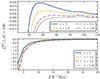 |
Fig. 1. Dipole model, including the contribution from nonlinear gravitational redshift. The top panel includes linear scales up to 120 h−1 Mpc, while the bottom panel is a zoom-in of the observable on nonlinear scales, up to 30 h−1 Mpc. In the two panels, we use a different range to display the dipole model for better visualization: the dipole amplitude is significantly larger on small scales. Specifics are taken from Table B.1, using the split 90% faint, 10% bright. Top and bottom panels focus on the large-scale and small-scale dipole predictions, respectively. |
Other models have been proposed in the literature, which use perturbation theory and include higher-order bias correction (Di Dio & Seljak 2019; Di Dio & Beutler 2020; Beutler & Di Dio 2020). The main disadvantage of this perturbative approach is that it introduces extra parameters into the model that cannot be directly measured in simulations but must instead be fitted to the simulated data vectors. The model presented in Saga et al. (2022) and outlined in this section is more predictive, primarily because the extra ingredients  and
and  can be estimated from simulations.
2.3. Theory covariance
The theory covariance for the linear dipole was first derived in Hall & Bonvin (2017). For the cross-correlation between two galaxy populations, there are three contributions: a pure shot noise term, a pure sample variance term, and a shot noise–sample variance cross-term:
 (18)
(18)
The shot noise term is given by
 (19)
(19)
the sample variance term can be written as
![Mathematical equation: $$ \begin{aligned} \mathrm{Cov}^{(\mathrm {SV})}_{ij}&= \frac{9}{4V}\left(\frac{\mathcal{H} }{\mathcal{H} _0}\right)^2\Bigg [\frac{2}{5} (b_{\rm F} \mathcal{C} _{\rm B} - b_{\rm B} \mathcal{C} _{\rm F})^2 \nonumber \\&\quad + \frac{4}{7} (\mathcal{C} _{\rm B} - \mathcal{C} _{\rm F}) (b_{\rm F} \mathcal{C} _{\rm B} - b_{\rm B} \mathcal{C} _{\rm F}) f + \frac{2}{9} (\mathcal{C} _{\rm B} - \mathcal{C} _{\rm F})^2 f^2\Bigg ]J_{ij} , \end{aligned} $$](/articles/aa/full_html/2025/02/aa52531-24/aa52531-24-eq36.gif) (20)
(20)
and the cross-term is
![Mathematical equation: $$ \begin{aligned} \mathrm{Cov}^{(\mathrm{SV}\,\times \,\mathrm{noise})}_{ij}&= \frac{9}{2\, V}\!\left[\frac{1}{\bar{n}_{\rm F}}\!\left(\frac{b_{\rm B}^2}{3}+\frac{2b_{\rm B} f}{5}+\frac{f^2}{7} \right) \right. \nonumber \\&\qquad \qquad \qquad \left.+\frac{1}{\bar{n}_{\rm B}}\!\left(\frac{b_{\rm F}^2}{3}+\frac{2b_{\rm F} f}{5}+\frac{f^2}{7} \right) \right]G_{ij}\,, \end{aligned} $$](/articles/aa/full_html/2025/02/aa52531-24/aa52531-24-eq37.gif) (21)
(21)
where V denotes the volume of the redshift bin,  is the average number density inside the bin, and Δd is the bin width used to estimate the correlation function. Here Gij and Jij are given by the following integrals of the linear matter power spectrum
 (22)
(22)
 (23)
(23)
In the upper panel of Fig. 2 we show the different contributions to the uncertainty estimated from the linear covariance by taking the square root of its diagonal elements at  . The sample variance term (SV) is largely subdominant on all scales. This is due to the fact that density and RSDs do not contribute to it – only relativistic effects affect this term. On scales larger than 15 h−1 Mpc, the uncertainty is mostly due to the cross term (SV × noise), which, contrary to the sample variance term, is affected by density and RSDs. In the highly nonlinear regime, d < 10 h−1 Mpc, the Poisson noise contribution dominates over the others. As shown in Saga et al. (2022), the theory covariance for the nonlinear model presented in Sect. 2.2 contains additional contributions from nonlinear gravitational redshift. However, they only affect the sample variance contributions and turn out to be negligible.
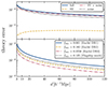 |
Fig. 2. Theory uncertainty, given by the square root of the diagonal elements of the theory covariance, estimated for the redshift bin |

In the lower panel of Fig. 2 we show how the theory uncertainty scales with respect to the sky coverage, assuming a fixed number density of galaxies. The theory uncertainty estimated for the Flagship mock is close to the uncertainty expected for the second data release of Euclid (DR2). We expect the uncertainty in Euclid DR3 to be reduced by about a factor 3/5 compared to the Flagship mock.
3. Method
3.1. Simulated data
3.1.1. The Flagship galaxy mock
The Euclid Flagship simulation (FS hereafter) is the reference simulation for the Euclid mission and it has been used as a key ingredient for the scientific preparation of the mission. The FS features a simulation box of 3600 h−1 Mpc on a side with 16 0003 particles, leading to a mass resolution of mp = 109 h−1 M⊙. This 4 trillion particle simulation is one of the largest N-body simulation performed to date and meets the basic science requirements of the mission: it allows us to include the faintest galaxies that Euclid will observe while sampling a cosmological volume comparable to what the Euclid Surveys will cover. The simulation is performed using PKDGRAV3 (Potter & Stadel 2016) on the ‘Piz Daint’ supercomputer at the Swiss National Supercomputing Centre (CSCS). The FS uses the following values for the density parameters: Ωm = 0.319, Ωb = 0.049, and ΩΛ = 0.681 − Ωrad − Ων, with a radiation density Ωrad = 0.00005509, and a contribution from massive neutrinos Ων = 0.00140343. Additional parameters are: the dark energy equation-of-state parameter w = −1.0, the reduced Hubble constant h = 0.67, the scalar spectral index of initial fluctuations ns = 0.96, and the amplitude of the scalar power spectrum As = 2.1 × 10⁻⁹ (corresponding to σ8 = 0.813) at k = 0.05 Mpc−1. The initial conditions are set at z = 99 using first-order Lagrangian perturbation theory (1LPT) displacements from a uniform particle grid. The transfer functions for the density field and the velocity field are generated at this initial redshift by CLASS (Lesgourgues 2011) and CONCEPT (Dakin et al. 2022).
The main data product are produced on the fly during the simulation and is a continuous full-sky particle light cone that extends to z = 3. The 3D particle light-cone data are used to identify roughly 150 billion dark matter haloes using Rockstar (Behroozi et al. 2013), and to create all-sky 2D maps of dark matter in 200 tomographic redshift shells between z = 0 and z = 99. The halo catalogue and the set of 2D dark matter maps are the main inputs for the Flagship mock galaxy catalogue. For a detailed description of the production of the catalogue, see Euclid Collaboration: Castander et al. (2025), but the main steps can be summarised as follows. First, galaxies are generated following a combination of halo occupation distribution (HOD) and abundance matching techniques. Following the HOD prescription, haloes are populated with central and satellite galaxies. Each halo contains a central galaxy and a number of satellites that depends on the halo mass. The halo occupation is chosen to reproduce observational constraints of galaxy clustering in the local Universe (Zehavi et al. 2011).
The luminosities of the central galaxies are assigned by performing abundance matching between the halo mass function of the simulation halo catalogue and the galaxy luminosity function (LF). The satellite luminosities are assigned assuming a universal Schechter LF in which the characteristic luminosity depends on the central luminosity in a way that ensures that the global LF agrees with observations. Galaxies are divided into three colour types, namely red, green, and blue, and the central and satellite galaxies in each group were distributed to match the clustering as a function of colour observed by Zehavi et al. (2011). The radial positions of the satellites within a given halo follow a best-fit ellipsoidal Navarro–Frenk–White (NFW) profile (Navarro et al. 1997). Finally, galaxy lensing properties are assigned within the Born approximation following the ‘onion universe’ approach presented in Fosalba et al. (2008) and Fosalba et al. (2015).
3.1.2. Selection of spectroscopic sample
We selected the spectroscopic catalogue from the Flagship simulation, version 2.1.10, in the following way. Objects were selected based on their Hα flux, with threshold FHα, lim = 2 × 10⁻¹⁶ erg cm−2 s−1. We considered two samples: a sample that only includes central galaxies and a sample with both central and satellite galaxies. The simulated data set covers a redshift range between zmin = 0.9 and zmax = 1.8, and we split it into four redshift bins, centred at  , with half-bin width
  . This is the binning that is used for the standard analysis of the spectroscopic sample of Euclid (Euclid Collaboration: Mellier et al. 2025). The properties of the objects within each of these redshift bins are summarised in Table 1. Galaxy bias and local count slope are estimated as described in Sect. 3.5.
Properties of the full catalogue.
The fraction of satellite galaxies in the catalogue ranges between 10% and 15% in the four redshift bins. Satellite galaxies are found preferentially in the proximity of the most massive haloes, and this results in a large galaxy bias when satellites are included, compared to the sample that only considers central galaxies. The values of the local count slope are only mildly affected by the presence of satellites.
3.2. Implementation of gravitational redshift in Flagship
In FS, the observed redshift is estimated from the peculiar velocities of galaxies. Other relativistic corrections, including gravitational redshift and the integrated Sachs–Wolfe effect, are neglected. In this work, to include the gravitational redshift zΨ = −Ψ/c2, we simply corrected the observed redshift zobs, FS provided in the Flagship catalogue by
 (24)
(24)
where  is the cosmological redshift, and we have neglected subdominant contributions.
To estimate the gravitational redshift we require the potential Ψ at each galaxy. Since on small scales the relativistic dipole is primarily sourced by gravitational redshift (Breton et al. 2019), it is important that the potential is accurately modelled on these scales. But given that high-resolution gravitational potential maps are not provided by the Flagship simulation, we adopted a semi-analytical approach and assumed that each halo where a galaxy is found can be modelled using a NFW density profile. The gravitational potential of the halo can then be estimated from the Poisson equation. The NFW gravitational potential Ψ ≡ ΨNFW at a comoving distance R from the centre of the halo is
 (25)
(25)
Here, ρs and Rs are the scale density and the scale radius, the two parameters that describe a NFW density profile. They depend on the concentration parameter, the virial radius, and the virial overdensity of the halo, see Mo et al. (2010) and Saga et al. (2022) for the exact expression of these quantities. For satellite galaxies, at a comoving distance R from the centre of the parent halo, we estimated the gravitational potential from Eq. (25). For the central galaxies, we took the limit
 (26)
(26)
This phenomenological model has been tested to be adequate for modelling the dipole (Saga et al. 2020, 2022).
3.3. Flux magnification
The measured fluxes of galaxies depend on the intrinsic luminosity of the object L and its luminosity distance DL by
 (27)
(27)
Since the luminosity distance is affected by perturbations (Bonvin et al. 2006; Challinor & Lewis 2011), the measured fluxes are also affected by relativistic effects such as magnification and Doppler corrections. While the observed fluxes in FS include observational effects such as dust extinction, magnification due to lensing and Doppler effects are not included. We corrected the fluxes to account for these effects using the relation
 (28)
(28)
where FFS are the fluxes stored in the mock, Fmagn are the magnified fluxes, and μL is the magnification factor due to gravitational lensing. This quantity can be expressed in terms of the convergence κ and shear γ = γ1 + i γ2:
 (29)
(29)
The fluxes Fmagn are therefore affected by gravitational lensing through μL and by Doppler effects and gravitational redshift through zobs.
3.4. Flux reference to perform split in bright and faint
The spectroscopic catalogue is constructed by selecting all objects based on their Hα flux. However, Euclid also measures the flux of galaxies in different colour bands, in particular the YE band, JE band, and HE band, see Euclid Collaboration: Jahnke et al. (2025), so performing this split using the Hα flux as reference is not necessarily the optimal choice. In order to determine which quantity is more suitable to split the catalogue in a bright and faint population, we checked the correlation between the fluxes and the mass of the parent halo.
In Fig. 3 we show the correlation of different galaxy fluxes, including the Hα flux, and the fluxes in the YE, JE, and HE bands, and the mass of the host halo. The top panels include only central objects, while the bottom panels include both central and satellite galaxies. Fluxes in infrared bands are more strongly correlated with the halo mass, especially for central galaxies. This is because these fluxes are correlated with the stellar mass of the galaxy, which is correlated to the halo mass. However, the Hα flux is correlated with the star-formation rate, which in general does not correlate with the mass of the host halo. For this reason, fluxes in the infrared bands are expected to be a better choice than the Hα flux to perform the split into bright and faint populations because they better trace the mass of the host halo. Bright objects in the infrared bands are more massive than the analogue selection applied to the Hα flux. Therefore, the former selection leads to larger differences in galaxy bias between faint and bright objects, consequently boosting some of the contributions to the dipole.
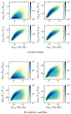 |
Fig. 3. Correlation of galaxy fluxes with the mass of the host halo. The top panel includes only central galaxies, the bottom panel includes both central and satellite galaxies. The reference fluxes are FHα0 = 1 erg cm−2 s−1 and FY0 = FJ0 = FH0 = 1 erg cm−2 s−1 Hz−1, while the reference halo mass is give by M0 = 1 h−1 M⊙, where M⊙ is the mass of the Sun. The colourbar highlights the density of objects in arbitrary units. |
In order to ensure that bright and faint populations have the same redshift evolution across all bins, we did not use a single flux cut. In fact, flux is inversely proportional to the square of the luminosity distance, meaning that a fixed flux cut would lead to more bright objects at low redshift and more faint objects at high redshift. To avoid this asymmetry in the redshift distribution, we performed the split in 20 sub-bins, following a similar procedure to the one described in Bonvin et al. (2023).
3.5. Estimation of biases
We describe here the method we used to estimate the galaxy bias and local count slope for the full Euclid spectroscopic sample, as well as for the bright and faint populations. In our analysis, we neglect the impact of evolution bias3.
3.5.1. Galaxy bias
The galaxy biases for the full and the bright/faint samples is estimated using the method described in Lepori et al. (2023) and Bonvin et al. (2023). We constructed a map of the galaxy number counts using HEALPix (Górski et al. 2005) and we extracted its angular power spectrum; we fitted it to a theory prediction of the power spectrum computed with the code CLASS (Di Dio et al. 2013, 2014b; Lesgourgues 2011; Blas et al. 2011), using HMCODE to account for nonlinear effects (Mead et al. 2016). The angular power spectrum of the map is estimated with the library NaMaster (Alonso et al. 2019), which corrects for the effect of the mask. The HEALPix map is constructed from the comoving position of the objects, and therefore its angular power spectrum only includes density contributions. Thus, we fitted the galaxy bias in real space, so included only the density term in our theory model. In the fit of the simulated spectrum to the model, we fixed the cosmology so that the only free parameter is the galaxy bias.
3.5.2. Local count slope
The local count slope for the entire sample is calculated from the slope of the cumulative LF of objects  , estimated at the flux limit (Bonvin et al. 2023).
The impact of flux magnification is more complex for the bright and faint populations, because the two samples are constructed by applying multiple flux cuts. Magnification from multiple flux selections has been first discussed in Borgeest et al. (1991). In Appendix A we derive an expression for the effective local count slope of the two populations, adapted to our case of interest, and we test the robustness of this method. Here we report the final result. Since bright and faint populations are the result of two flux selections, first in Hα flux and, second, in YE-band flux, we expect that for both populations, magnification can change the count of objects in two ways: moving objects across the threshold FHα, lim to the faint or bright population, and transferring objects from the faint to the bright population across the threshold FYE, lim. This is shown schematically in Fig. A.1. Therefore, we can define an effective count slope for the bright and faint population as the sum of two contributions,
 (30)
(30)
where
 (31)
(31)
and we introduce the LF of bright and faint galaxies in the redshift bin  , that is
  and
and  , respectively. The luminosities
  are the luminosities corresponding to the flux FX in the background FLRW cosmology.
Since across the flux cut FY, lim objects are transferred from the bright to the faint catalogue and vice versa, sF, YE and sB, YE are not independent, that is,
 (32)
(32)
In practice, we estimated the slopes sB/F, Hα by fixing the flux cuts in the YE band and performing the same cuts on a version of the mock that is deeper in Hα flux. The slope sB, YE is estimated after applying the selection in the Hα flux, from the cumulative LF of the bright population at the flux cut in the YE band. Since we performed the split between bright and faint in sub-bins, the YE-band flux cut is redshift dependent. We estimated the slope of the cumulative LF in sub-bins and estimated an effective value by taking an average weighted by the number of objects in each sub-bin.
3.6. Measurements of the dipole and its covariance
We used the Landy–Szalay (LS) estimator (Landy & Szalay 1993) to measure the 3D cross-correlation between bright and faint objects within each redshift bin,
 (33)
(33)
This pair count-based estimator requires introducing two Poisson-sampled random catalogues, RB and RF, that mimic the redshift distribution of the respective bright (DB) and faint (DF) data catalogues but have a uniform distribution in the solid angle. The XYBF in Eq. (33) are then histograms of pair counts between catalogue XB and catalogue YF, binned in d and μ and normalised by their total number of pairs, i.e., the pair counts in each bin are divided by the product of the number of objects in catalogue XB and the number of objects in catalogue YF.
The LS estimator has been shown to have the lowest possible variance and bias among all possible estimators based on pair counts, if the correlation is small (ξ ≪ 1) and if the number densities of the random catalogues are sufficiently high (Landy & Szalay 1993; Kerscher et al. 2000; Keihänen et al. 2019). In order to get unbiased results, we hence created random catalogues that have ten times as many objects as their corresponding data catalogues.
In practice, we created the Poisson-sampled random catalogues from the density distribution of the data catalogues using the inversion method, as described in Schulz (2023). The LS estimator is computed using a modified version of the publicly available code CUTE (Alonso 2012). The modifications, which are the same as in Breton et al. (2019), extend the capabilities of CUTE to allow the computation of odd multipoles in the two-point correlation function. We counted the pairs for separations 2 h−1 Mpc ≤ d ≤ 30 h−1 Mpc and orientations −1 ≤ μ ≤ 1, binning into d-bins of width Δd = 2 h−1 Mpc and μ-bins of width Δμ = 0.004.
We did not estimate the correlation for smaller separations because such separations are not well sampled by our catalogues. The average separation between a bright object and the closest faint object can be derived from the cross-correlation function monopole, as it represents the average overdensity of faint objects in the neighbourhood of a bright object. From the measurements of the real-space monopoles on the light cone at small separations we found that there are typically no faint objects separated by d ≲ 1 h−1 Mpc from the average bright object, and at  , the average separation between a bright and the closest faint object is d = 3.6 h−1 Mpc. The number of pairs with separation below this value is generally small, leading to very large Poisson errors on the measurement at those separations. Additionally, at very small separations, the LS estimator can in principle become undefined in certain (d, μ)-bins if there are no pairs between the two random catalogues. For these reasons, we excluded d < 2 h−1 Mpc from the analysis.
The ℓ-th multipole of the LS estimator is defined by the relation
 (34)
(34)
In practice, the integral is numerically computed as a sum over the μ-bins. We thus computed the dipole of the LS estimator as
 (35)
(35)
The covariance of the measurement was estimated with the jackknife (JK) method (Norberg et al. 2009),
![Mathematical equation: $$ \begin{aligned} \mathrm{Cov}^\mathrm{JK}_{ij}&:= \mathrm{Cov}^\mathrm{JK}\left(\xi _1(\bar{z}, d_i),\xi _1(\bar{z},d_j)\right)\\&= \frac{(N-1)}{N}\sum ^N_{k=1}\left[\xi ^k_1(\bar{z}, d_i) - \bar{\xi }_1(\bar{z},d_i)\right]\left[\xi ^k_1(\bar{z},d_j) - \bar{\xi }_1(\bar{z},d_j)\right] ,\nonumber \end{aligned} $$](/articles/aa/full_html/2025/02/aa52531-24/aa52531-24-eq65.gif) (36)
(36)
where the survey volume at redshift  was divided into N = 50 sub-volumes with approximately equal surface area and shape by running a KMEANS4 algorithm (Kwan et al. 2017; Suchyta et al. 2016) on one of the corresponding random catalogues. The same split was applied to the data catalogues and the LS dipole was measured N times, each time removing a different sub-volume k from the survey. In Eq. (36),
  is the dipole measured within the survey volume at redshift
  from which the k-th sub-volume has been removed, and
  is the JK sample mean,
 (37)
(37)
We confirmed that increasing the number of sub-volumes from 50 to 100 does not change the estimated covariance. We conclude that with 50 JK regions, the JK covariance is already well converged and is thus a robust estimate of the measurement covariance.
In Fig. 4 we compare the uncertainty estimate from the JK and the theory covariance. The theory covariance underestimates the uncertainty on all scales. In the redshift bin centred at  , the discrepancy between the JK and theory covariance ranges between 10% and 20% on scales larger than 10 h−1 Mpc, while on smaller scales, the uncertainty estimated from our mock is up to a factor of two larger than the theory uncertainty. This difference is even larger at higher redshift. In the nonlinear regime, the JK covariance provides a significantly more conservative forecast for the detection significance.
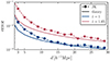 |
Fig. 4. Comparison of the uncertainty estimate from the theory covariance (continuous lines) and numerical covariance, computed from the mock using the JK resampling method (data points). We consider the two representative redshift bins centred at |


3.7. Method to estimate the significance of the detection
Given a set of observations for the dipole and its theoretical prediction, we want to provide a quantitative estimate of its detection. To do this, we determined the detection in units of σ as the difference in χ2 between accepting or rejecting the presence of the dipole. In practice, we considered the following χ2 when we include a dipole in our prediction,
 (38)
(38)
where i and j run over different separation bins,  stands for the theoretical prediction of the dipole,
  represents its estimate from observed data, and cov corresponds to the covariance, which can be the theoretical covariance, the JK covariance, or their combination.
We further considered the χ2 when no dipole is added into the prediction,
 (39)
(39)
The detection significance in units of σ can then be expressed as
![Mathematical equation: $$ \begin{aligned} \text{ detection}\,[\sigma ]=\sqrt{\Delta \chi ^2}=\sqrt{\chi ^2_{\rm no\,dipole}-\chi ^2_{\rm dipole}}\,. \end{aligned} $$](/articles/aa/full_html/2025/02/aa52531-24/aa52531-24-eq78.gif) (40)
(40)
It is important to note that the computation of the detection significance requires the inversion of the covariance matrix. However, JK covariances may contain a non-negligible level of noise, which can lead to biased results. We corrected for this by applying the Hartlap factor (Hartlap et al. 2007). In more detail, we multiplied the inverse covariance matrix by (NJK − p − 2)/(NJK − 1), where NJK stands for the number of JK regions and p represents the number of separation bins.
4. Results
In this section, we report the main results of the paper.
In Sect. 4.1 we discuss the signal-to-noise ratio (S/N) of the relativistic dipole in the linear regime. In Sect. 4.2 we present the measurement of the dipole from the Flagship simulation on small scales, for separations smaller than 30 h−1 Mpc. We consider two ways of splitting the catalogue of Euclid into a bright and faint population, and we report the significance of detection for these two cases. In Sect. 4.3 we isolate the different contributions to the dipole and discuss the contribution of nonlinear velocities. In Sect. 4.4 we investigate the impact of satellite objects and flux magnification on the significance of detection.
In Table B.1 we report the details for two representative splits considered in this work: a case with 90% of faint objects and 10% of bright objects, and a case with 50% of bright and faint objects. The table shows the number of objects in each redshift bin, the galaxy bias and local count slope estimates, and the mean gravitational potential at the position of the galaxy. These quantities have been used to compute the theory model in the linear and nonlinear regime and to estimate the theory covariance. We report the measurements for our selection of objects including only central galaxies, as well as both central and satellite galaxies.
4.1. Relativistic dipole in the linear regime
As a preliminary study, we examine the expected S/N of the dipole for the spectroscopic catalogue of Euclid on large scales. The S/N is estimated in each redshift bin as
\,\, \xi _{1}(\bar{z}_i, d_k) }\,, \end{aligned} $$](/articles/aa/full_html/2025/02/aa52531-24/aa52531-24-eq79.gif) (41)
(41)
where the dipole  and covariance Cov[ξ1j,ξ1k], given by Eq. (18), are both computed using linear theory. We evaluate Eq. (41) including separations between dmin ≡ 20 h−1 Mpc and dmax ≡ 200 h−1 Mpc, and a bin width Δd = 2 h−1 Mpc. We use the sky coverage of the Flagship simulation (fsky = 0.125).
In Fig. 5 we show the S/N as a function of the mean redshift, for a range of splits with different percentages of bright and faint objects. The S/N increases as we increase the percentage of faint objects; these configurations maximise the differences between biases. We find that the S/N is larger in the low-redshift bins. However, for all configurations and redshifts, we find a S/N < 1, which indicates that we cannot detect the dipole in the catalogue of Euclid in the linear regime. This is not so surprising: the linear model of the dipole contains a Doppler term ∼c/(rℋ) that boosts the signal-to-noise ratio at low redshift but decays at high redshift. The forecast shown in Fig. 5 includes only central objects. We checked that including satellite galaxies does not change this picture substantially. We also verified that measurements of the dipole from the Flagship simulation on large scales are consistent with zero within their error bars. Since the relativistic dipole is not detectable by Euclid on large scales, the rest of this analysis focuses on the nonlinear regime.
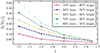 |
Fig. 5. S/N of the dipole on linear scales (≥20 h−1 Mpc) for a range of population splits. Here the model prediction is given by linear theory. |
4.2. Relativistic dipole in the nonlinear regime
In this section, we present the measurements of the relativistic dipole on small scales from the Flagship simulation. We split the spectroscopic mock catalogue into two populations based on the Y-band flux of the objects, as described in Sect. 3.4. We consider two representative cases: a split with equal numbers of bright and faint objects (50%–50% case) and a split with 10% of bright objects and 90% of faint objects (10%–90% case).
In Fig. 6 we show the measurement of the dipole in the four redshift bins at  , for the 50%–50% case (left panels) and 10%–90% case (right panels). The catalogue processed to obtain these measurements only contains central galaxies, and we neglect flux magnification. The predictions of theory is estimated from the model in Sect. 2.2, which assumes that the kinematic contributions to the dipole are adequately modelled using linear theory, with nonlinearities mainly affecting the gravitational redshift contribution. The specifics of the galaxy populations (galaxy bias and mean gravitational potential at the galaxy position) are estimated from the catalogues and their values are reported in Table B.1.
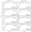 |
Fig. 6. Measurements of the dipole on small scales, compared to the phenomenological theory model described in Sect. 2.2. The left panels refer to the 50%–50% split, the right panels refer to the 10%–90% split. The rows from top to bottom correspond to the measurements at redshift |

The data points agree with the prediction of the theory roughly within two standard deviations on scales d ≥ 3 h−1 Mpc for both cases. The fact that the first data point at d = 1 h−1 Mpc is rather off compared to the theory prediction is not that surprising, as very few pairs of bright and faint objects are found at this separation.
As expected, in the 50%–50% case, we find that the amplitude of the signal is smaller compared to the 10%–90% case. However, the errors in the measurements are larger in the 10%–90% case due to larger shot noise in the reduced bright sample. To assess which split gives an overall better S/N, we follow the method described in Sect. 3.7 to quantify the significance of detection in the two cases. In Table 2 we report the values of the detection significance for three possible choices for the covariance: the theory covariance, the JK covariance, and a combination of the two. The combined covariance is constructed as (see, e.g., Bonvin et al. 2023)
Detection significance.
 (42)
(42)
where  is the theory correlation matrix, given by
 (43)
(43)
and i and j run over the components of the covariance matrix. The combined covariance provides the same error estimate as the JK method, having the advantage that the non-diagonal elements do not exhibit spurious numerical oscillations and follow the trend expected from the theory covariance. Assuming the measurements in different redshift bins are independent, we also computed the total detection significance by summing in quadrature the significance of all bins. The first data point at d = 1 h−1 Mpc is excluded from this analysis.
The JK covariance and the combined covariance give roughly consistent results, forecasting a detection significance between 3σ and 4σ in the redshift bins  and a detection significance ≲2σ at higher redshift. The total detection significance amounts to 5σ–6σ. Overall, the 10%–90% split leads to slightly better detection significance. Therefore, in the remainder of this paper, we consider this case our baseline. The theory covariance gives a considerably better detection significance, ranging between 11σ (50%–50% split) and 13σ (10%–90% split), when all the redshift bins are combined. As a conservative choice, we consider the combined covariance as the fiducial.
The estimation of the detection significance assumes perfect knowledge of the linear galaxy bias of the two populations. While we can measure this quantity very accurately in simulations, where the underlying cosmological model is known, this will not be possible with the Euclid real data. This issue can be overcome by considering a joint analysis of the even multipoles of both galaxy populations combined with the dipole measurement, leaving the galaxy bias as free parameters in the analysis. It is shown in Sobral-Blanco & Bonvin (2022) that the bias of the bright and faint populations are typically very well constrained by the even multipoles and that the uncertainty on the biases barely impacts the measurement of gravitational redshift. More precisely, comparing the detectability of gravitational redshift with the detectability of gravitational redshift multiplied by the bias difference bB − bF leads to a difference in precision of 0.1%. This shows that even if the bias difference is fully degenerated with the gravitational redshift signal in the dipole, the biases are so well constrained by the even multipoles that the degeneracy can be extremely well broken.
4.3. Isolating the different contributions to the dipole
In this section, we study the different physical effects that contribute to the nonlinear dipole. We adopt the baseline split (10%–90%). In order to isolate Doppler effects and gravitational redshift, we measure the dipole from the Flagship catalogue including different contributions to the observed redshift. We consider the following combinations: a) the only contribution to the redshift comes from the Hubble expansion (background redshift), b) we include only the effect of peculiar velocities (and neglect gravitational redshift), c) we include only the effect of gravitational redshift, and d) we include both peculiar velocities and gravitational redshift.
Note that case a) does not completely remove the effect of peculiar velocities on the dipole due to the so-called light-cone effect (Kaiser 2013; Bonvin et al. 2014; Breton et al. 2019). This arises because the rate (in terms of look-back time, for example) at which a light ray intercepts sources depends on the peculiar motion of the sources, and it is higher when the sources move towards the light ray (away from the observer). This information is carried back to the observer, who consequently sees an enhanced (suppressed) number density in regions where sources are moving away from (towards) the observer. For example, on the near side of a cluster where infalling galaxies move away from us, the density is seen to be higher, whereas on the far side it is lower. The overall effect is a dipole (which is opposite in sign to the one from the gravitational redshift). Thus, all a), b), c), and d) are affected by the light-cone effect but only b) and d) explicitly include the Doppler contribution to the redshift.
In Fig. 7 we show the measurements for a) and b) in the left panels, and for c) and d) in the right panels, compared to our theory prediction that includes linear velocities and nonlinear gravitational potential. The two contributions of peculiar velocities, coming from the light-cone and Doppler effects, are individually consistent with zero at  . In the redshift bin
  , the light-cone effect is not completely negligible, as the dipole measurements exhibit a systematic negative amplitude on scales below 10 h−1 Mpc. However, the combined Doppler and light-cone effects lead to a dipole consistent with zero on scales > 3 h−1 Mpc. This suggests that at
  the contributions from nonlinear Doppler effects and the light-cone effects are individually not negligible. However, since they generate a dipole of opposite sign, their combined contribution is consistent with zero on scales > 3 h−1 Mpc. Since both of these effects are coupled to the gravitational redshift in the full dipole measurements, we cannot robustly conclude that the effect of nonlinear peculiar velocities is negligible at
  , where we forecast the greater detection significance. A model that can consistently treat both nonlinear velocities and nonlinear gravitational potential is needed for a correct interpretation of the dipole measurement at these scales.
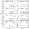 |
Fig. 7. Measurements of the dipole isolating different contributions, using the 10% bright – 90% faint split. In the left panels, we show the ‘light cone’ data points from the catalogue using the background redshift to perform both selection and measurements, while ‘Doppler + light cone’ uses the redshift corrected by the peculiar velocities of the galaxies. In the right panels, ‘gravitational redshift + light cone’ uses a redshift that includes gravitational redshift but does not account for the peculiar motion of the sources, and the measurements labelled as ‘all’ include both peculiar velocities and gravitational redshift. The theory predictions (red continuous lines) represent our fiducial theory model, which incorporates linear velocities and nonlinear gravitational redshift. Rows from top to bottom correspond to measurements at redshift |

4.4. Impact of satellite galaxies and flux magnification
In our baseline settings, we have only included central galaxies, and we have neglected flux magnification. In this section, we discuss the impact of satellite galaxies and flux magnification on the dipole measurements, which includes both the Doppler and the subdominant contribution from lensing magnification.
We performed the dipole measurements for our baseline split (10%–90%) including satellite objects in the sample (and neglecting flux magnification). The specifics for the catalogues with satellites are reported in Table B.1. Compared to the selection with only central objects, including satellites results in a larger number of objects, larger galaxy bias, and higher average gravitational potential at the positions of the sources for both populations. This is because satellite galaxies are primarily found inside the most massive haloes of the simulation.
In the left panels of Fig. 8 we compare the dipole measurements and theory prediction for the cases with and without satellite galaxies. Both measurements and theory prediction change very little when satellite objects are included. In Table 3 we report the detection significance for measurements with satellite objects (second column). We see that the detection significance is systematically slightly decreased in all redshift bins. However, this does not change the outcome of the analysis substantially: we forecast a detection significance of ≈4σ and ≈3σ in the bins centred at  and
and  , respectively. At higher redshift, the detection significance is below 2σ.
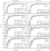 |
Fig. 8. Impact of satellite galaxies (left panels) and flux magnification (right panels) on the measurements, for the 10% bright – 90% faint split. Since in our fiducial model velocities are treated linearly, flux magnification has a negligible impact on the theory prediction. Rows from top to bottom correspond to measurements at redshift |
We perform a similar analysis to test the impact of flux magnification. In the right panels of Fig. 8 we compare the dipole measurements for the cases with and without flux magnification. Flux magnification does not affect the gravitational redshift contribution to the dipole, and since this is by far the largest contribution to our prediction, its impact on the theory model is largely negligible. The measured dipole for the catalogues with flux magnification is consistent with the measurements without flux magnification. In Table 3 we report the significance of the detection for these measurements. We find that it is compatible with the estimate for our baseline setting, with only central galaxies and no flux magnification. The differences between the two cases are ≤0.3σ in all redshift bins.
Impact of satellite galaxies and flux magnification on the detection significance.
Overall, we find that including satellites or flux magnification does not change the outcome of the analysis in a relevant way.
5. Conclusions
In this paper, we present a measurement of the dipole of the two-point correlation function in the Flagship simulation, for a selection of objects tailored to the Euclid Spectroscopic Survey. This observable is sourced by gravitational redshift and Doppler effects, and it has been shown that it can be used to test the equivalence principle on cosmological scales, see, for example, Bonvin & Fleury (2018).
Since the contribution of gravitational redshift to the observed redshift is not currently included in the Flagship mock, we implemented this effect by modelling the gravitational potential at the position of each galaxy using the NFW profile for the host haloes. In order to isolate these relativistic effects from the standard clustering contributions, given by the galaxy overdensity and RSDs, we split the full sample of galaxies into two populations. The split is performed using their fluxes in the YE band as reference. We show that this choice leads to larger differences in galaxy bias for the bright and faint sample, being more correlated with the mass of the host halo than the Hα flux. On large scales, the dipole measured from the Flagship mock is consistent with zero regardless of the percentage of bright and faint objects. This is not surprising, as a signal-to-noise analysis based on linear theory leads to S/N < 1. On small scales, the amplitude of the signal is significantly larger due to the contributions of nonlinear gravitational redshift. Using the model presented in Saga et al. (2020, 2022) as a reference, on scales d < 30 h−1 Mpc and for our fiducial split with 90% faint objects and 10% bright objects, we found a detection significance of 4.5σ, 3.7σ, 1.5σ, and 2.1σ in the four redshift bins  , respectively. The overall detection significance amounts to 6σ. These values are obtained from the combined covariance, which rescales the analytical covariance to match the uncertainty estimated from the mock using the JK method. This is our fiducial choice, which leads to a conservative estimate. A split with equal number of bright and faint objects leads to a slightly lower detection significance at low redshift.
While our nonlinear model accounts for nonlinear gravitational redshift, it models velocities using linear theory. We tested this assumption by separating the different contributions to the dipole: the light-cone effect, the sum of light-cone and Doppler effects, and the gravitational redshift. Although the gravitational redshift is the largest contribution to the nonlinear dipole, the light-cone effect is not completely negligible at  . Nevertheless, the contributions from light-cone and Doppler effects appear to roughly cancel out. We cannot interpret this cancellation in our nonlinear model, since it only models velocities using linear theory. To correctly separate the different contributions to the dipole at low redshift and on small scales, we require a model that can consistently treat both the nonlinearities in the velocities and the gravitational potential (see, e.g., Dam & Bonvin 2023). We leave the development of a complete nonlinear model to future work.
We also studied the impact of satellite galaxies and flux magnification on the estimated dipole, finding that the detection significance of the dipole is not substantially affected by them. Although flux magnification has negligible impact on our measurements, in Appendix A we validate different methods to estimate the local count slope for selections with multiple flux cuts. This work is relevant for modelling lensing magnification in galaxy clustering when the selection of galaxies is not a simple flux cut. The measurements in the Flagship mock catalogue cover 1/8 of the sky, which roughly corresponds to 5000 deg2. This is about twice the sky coverage planned for Euclid DR1. Assuming that the number density and galaxy bias of the Flagship mock reflects the properties of the galaxies observed by Euclid in all the three planned Data Releases (Euclid Collaboration: Scaramella et al. 2022; Euclid Collaboration: Mellier et al. 2025), we forecast that a detection of the dipole is foreseeable for DR2 and DR3. In estimating the detection significance of the dipole, we have assumed that the Euclid spectroscopic sample is pure and complete. A detailed analysis accounting for these effects and other systematic uncertainties is left for future work.
While we include in our measurements scales d < 30 h−1 Mpc, we point out that most of the signal-to-noise comes from separations d ∼ 5 h−1 Mpc. This is the typical scale at which gravitational redshift has been detected in galaxy clusters; see, for example, Wojtak et al. (2011), Sadeh et al. (2015), and Rosselli et al. (2023). The key observable in these measurements is the distribution of line-of-sight (LOS) velocities for cluster member galaxies around the cluster centre: the kinematic Doppler effect gives rise to a broad symmetric distribution around a zero LOS velocity, while gravitational redshift shifts the value of the mean velocity of this distribution. Compared to the cluster measurements, the method we propose has the advantage of not requiring the identification of cluster member galaxies or associating the cluster centre with a specific galaxy in the spectroscopic catalogue. Measuring the galaxy cross-correlation function is, in a way, more general, as various splitting strategies can be tested and combined to optimise the measurements. The different systematics affecting the two observables make them highly complementary. A quantitative comparison between the two approaches would require forecasting the detectability of gravitational redshift in the Euclid cluster catalogue (Sartoris et al. 2016; Euclid Collaboration: Adam et al. 2019), which is beyond the scope of this work.
We adopt Einstein’s summation convention in which repeated indices are summed over.
This assumption is violated in presence of a fifth force acting on the dark matter component; see, for example, Bonvin & Fleury (2018).
Our galaxy selection leads to the same observed redshift evolution of the two populations and partially cancels out the dipole contribution of source count evolution, which is proportional to the difference in the evolution biases of the two populations. Neglecting evolution bias is also fully justified by the outcome of our analysis in Sect. 4.1, where we show that the overall linear dipole is very small.
The luminosities  are the luminosities corresponding to the flux FX in the background.
Acknowledgments
The work of FL, SS, JA, and CB is supported by the Swiss National Science Foundation. CB and LD acknowledge support from the European Research Council (ERC) under the European Union’s Horizon 2020 research and innovation program (grant agreement No. 863929; project title “Testing the law of gravity with novel large-scale structure observables”). The Euclid Consortium acknowledges the European Space Agency and a number of agencies and institutes that have supported the development of Euclid, in particular the Agenzia Spaziale Italiana, the Austrian Forschungsförderungsgesellschaft funded through BMK, the Belgian Science Policy, the Canadian Euclid Consortium, the Deutsches Zentrum für Luft- und Raumfahrt, the DTU Space and the Niels Bohr Institute in Denmark, the French Centre National d’Etudes Spatiales, the Fundação para a Ciência e a Tecnologia, the Hungarian Academy of Sciences, the Ministerio de Ciencia, Innovación y Universidades, the National Aeronautics and Space Administration, the National Astronomical Observatory of Japan, the Netherlandse Onderzoekschool Voor Astronomie, the Norwegian Space Agency, the Research Council of Finland, the Romanian Space Agency, the State Secretariat for Education, Research, and Innovation (SERI) at the Swiss Space Office (SSO), and the United Kingdom Space Agency. A complete and detailed list is available on the Euclid website (https://www.euclid-ec.org/). This work has made use of CosmoHub (Tallada et al. 2020; Carretero et al. 2017). CosmoHub has been developed by the Port d’Informacio Cientifica (PIC), maintained through a collaboration of the Institut de Fisica d’Altes Energies (IFAE) and the Centro de Investigaciones Energeticas, Medioambientales y Tecnologicas (CIEMAT) and the Institute of Space Sciences (CSIC & IEEC). CosmoHub was partially funded by the “Plan Estatal de Investigacion Cientifica y Tecnica y de Innovacion” program of the Spanish government, has been supported by the call for grants for Scientific and Technical Equipment 2021 of the State Program for Knowledge Generation and Scientific and Technological Strengthening of the R+D+i System, financed by MCIN/AEI/ 10.13039/501100011033 and the EU NextGeneration/PRTR (Hadoop Cluster for the comprehensive management of massive scientific data, reference EQC2021-007479-P) and by MICIIN with funding from European Union NextGenerationEU(PRTR-C17.I1) and by Generalitat de Catalunya.
References
- Abbott, T. M. C., Aguena, M., Alarcon, A., et al. 2022, Phys. Rev. D, 105, 023520 [CrossRef] [Google Scholar]
- Alam, S., Ho, S., & Silvestri, A. 2016, MNRAS, 456, 3743 [Google Scholar]
- Alam, S., Zhu, H., Croft, R. A. C., et al. 2017, MNRAS, 470, 2822 [NASA ADS] [CrossRef] [Google Scholar]
- Alam, S., Aubert, M., Avila, S., et al. 2021, Phys. Rev. D, 103, 083533 [NASA ADS] [CrossRef] [Google Scholar]
- Alonso, D. 2012, ArXiv e-prints [arXiv:1210.1833] [Google Scholar]
- Alonso, D., Sanchez, J., & Slosar, A. 2019, MNRAS, 484, 4127 [Google Scholar]
- Amendola, L., Appleby, S., Bacon, D., et al. 2018, Living Rev. Rel., 21, 2 [NASA ADS] [CrossRef] [Google Scholar]
- Behroozi, P. S., Wechsler, R. H., & Wu, H.-Y. 2013, ApJ, 762, 109 [NASA ADS] [CrossRef] [Google Scholar]
- Bermejo-Climent, J. R., Ballardini, M., Finelli, F., & Cardone, V. F. 2020, Phys. Rev. D, 102, 023502 [NASA ADS] [CrossRef] [Google Scholar]
- Bertacca, D., Maartens, R., & Clarkson, C. 2014, JCAP, 09, 037 [Google Scholar]
- Beutler, F., & Di Dio, E. 2020, JCAP, 07, 048 [CrossRef] [Google Scholar]
- Blas, D., Lesgourgues, J., & Tram, T. 2011, JCAP, 07, 034 [CrossRef] [Google Scholar]
- Bonvin, C. 2014, Class. Quant. Grav., 31, 234002 [NASA ADS] [CrossRef] [Google Scholar]
- Bonvin, C., & Durrer, R. 2011, Phys. Rev. D, 84, 063505 [NASA ADS] [CrossRef] [Google Scholar]
- Bonvin, C., & Fleury, P. 2018, JCAP, 05, 061 [CrossRef] [Google Scholar]
- Bonvin, C., & Pogosian, L. 2023, Nature Astron., 7, 1127 [NASA ADS] [CrossRef] [Google Scholar]
- Bonvin, C., Durrer, R., & Gasparini, M. A. 2006, Phys. Rev. D, 73, 023523 [Erratum: Phys. Rev. D 85, 029901 (2012)] [Google Scholar]
- Bonvin, C., Hui, L., & Gaztañaga, E. 2014, Phys. Rev. D, 89, 083535 [NASA ADS] [CrossRef] [Google Scholar]
- Bonvin, C., Hui, L., & Gaztañaga, E. 2016, JCAP, 08, 021 [CrossRef] [Google Scholar]
- Bonvin, C., Lepori, F., Schulz, S., et al. 2023, MNRAS, 525, 4611 [NASA ADS] [CrossRef] [Google Scholar]
- Borgeest, U., von Linde, J., & Refsdal, S. 1991, A&A, 251, L35 [NASA ADS] [Google Scholar]
- Breton, M.-A., Rasera, Y., Taruya, A., Lacombe, O., & Saga, S. 2019, MNRAS, 483, 2671 [NASA ADS] [CrossRef] [Google Scholar]
- Carretero, J., Tallada, P., Casals, J., et al. 2017, in Proceedings of the European Physical Society Conference on High Energy Physics. 5–12 July, 488 [CrossRef] [Google Scholar]
- Castello, S., Grimm, N., & Bonvin, C. 2022, Phys. Rev. D, 106, 083511 [CrossRef] [Google Scholar]
- Castello, S., Mancarella, M., Grimm, N., et al. 2024, JCAP, 05, 003 [CrossRef] [Google Scholar]
- Challinor, A., & Lewis, A. 2011, Phys. Rev. D, 84, 043516 [NASA ADS] [CrossRef] [Google Scholar]
- Dakin, J., Hannestad, S., & Tram, T. 2022, MNRAS, 513, 991 [CrossRef] [Google Scholar]
- Dam, L., & Bonvin, C. 2023, Phys. Rev. D, 108, 103505 [NASA ADS] [CrossRef] [Google Scholar]
- DES Collaboration (Abbott, T. M. C., et al.) 2024, ApJ, 973, L14 [NASA ADS] [CrossRef] [Google Scholar]
- DESI Collaboration (Adame, A. G., et al.) 2024, JCAP, accepted [arXiv:2404.03002] [Google Scholar]
- Di Dio, E., & Beutler, F. 2020, JCAP, 09, 058 [CrossRef] [Google Scholar]
- Di Dio, E., & Seljak, U. 2019, JCAP, 04, 050 [CrossRef] [Google Scholar]
- Di Dio, E., Montanari, F., Lesgourgues, J., & Durrer, R. 2013, JCAP, 11, 044 [CrossRef] [Google Scholar]
- Di Dio, E., Durrer, R., Marozzi, G., & Montanari, F. 2014a, JCAP, 12, 017 [Erratum: JCAP 06, E01 (2015)] [Google Scholar]
- Di Dio, E., Montanari, F., Durrer, R., & Lesgourgues, J. 2014b, JCAP, 01, 042 [CrossRef] [Google Scholar]
- Di Valentino, E., Anchordoqui, L. A., Akarsu, Özgür, et al. 2021a, Astropart. Phys., 131, 102604 [NASA ADS] [CrossRef] [Google Scholar]
- Di Valentino, E., Anchordoqui, L. A., Akarsu, Özgür, et al. 2021b, Astropart. Phys., 131, 102605 [NASA ADS] [CrossRef] [Google Scholar]
- Euclid Collaboration (Adam, R., et al.) 2019, A&A, 627, A23 [NASA ADS] [CrossRef] [EDP Sciences] [Google Scholar]
- Euclid Collaboration (Lepori, F., et al.) 2022, A&A, 662, A93 [NASA ADS] [CrossRef] [EDP Sciences] [Google Scholar]
- Euclid Collaboration (Scaramella, R., et al.) 2022, A&A, 662, A112 [NASA ADS] [CrossRef] [EDP Sciences] [Google Scholar]
- Euclid Collaboration (Jelic-Cizmek, G., et al.) 2024, A&A, 685, A167 [NASA ADS] [CrossRef] [EDP Sciences] [Google Scholar]
- Euclid Collaboration (Castander, F. J., et al.) 2025, A&A, in press, https://doi.org/10.1051/0004-6361/202450853 [Google Scholar]
- Euclid Collaboration (Jahnke, K., et al.) 2025, A&A, in press, https://doi.org/10.1051/0004-6361/202450786 [Google Scholar]
- Euclid Collaboration (Mellier, Y., et al.) 2025, A&A, in press, https://doi.org/10.1051/0004-6361/202450810 [Google Scholar]
- Fosalba, P., Gaztañaga, E., Castander, F. J., & Manera, M. 2008, MNRAS, 391, 435 [NASA ADS] [CrossRef] [Google Scholar]
- Fosalba, P., Gaztañaga, E., Castander, F. J., & Crocce, M. 2015, MNRAS, 447, 1319 [NASA ADS] [CrossRef] [Google Scholar]
- Górski, K. M., Hivon, E., Banday, A. J., et al. 2005, ApJ, 622, 759 [Google Scholar]
- Hall, A., & Bonvin, C. 2017, Phys. Rev. D, 95, 043530 [CrossRef] [Google Scholar]
- Hartlap, J., Simon, P., & Schneider, P. 2007, A&A, 464, 399 [NASA ADS] [CrossRef] [EDP Sciences] [Google Scholar]
- Hildebrandt, H. 2016, MNRAS, 455, 3943 [NASA ADS] [CrossRef] [Google Scholar]
- Hinshaw, G., Larson, D., Komatsu, E., et al. 2013, ApJS, 208, 19 [Google Scholar]
- Jelic-Cizmek, G., Lepori, F., Bonvin, C., & Durrer, R. 2021, JCAP, 04, 055 [NASA ADS] [CrossRef] [Google Scholar]
- Jeong, D., Schmidt, F., & Hirata, C. M. 2012, Phys. Rev. D, 85, 023504 [NASA ADS] [CrossRef] [Google Scholar]
- Kaiser, N. 1987, MNRAS, 227, 1 [Google Scholar]
- Kaiser, N. 2013, MNRAS, 435, 1278 [NASA ADS] [CrossRef] [Google Scholar]
- Keihänen, E., Kurki-Suonio, H., Lindholm, V., et al. 2019, A&A, 631, A73 [NASA ADS] [CrossRef] [EDP Sciences] [Google Scholar]
- Kerscher, M., Szapudi, I., & Szalay, A. S. 2000, ApJ, 535, L13 [NASA ADS] [CrossRef] [Google Scholar]
- Kwan, J., Sánchez, C., Clampitt, J., et al. 2017, MNRAS, 464, 4045 [NASA ADS] [CrossRef] [Google Scholar]
- Landy, S. D., & Szalay, A. S. 1993, ApJ, 412, 64 [Google Scholar]
- Laureijs, R., Amiaux, J., Arduini, S., et al. 2011, ArXiv e-prints [arXiv:1110.3193] [Google Scholar]
- Lepori, F., Di Dio, E., Villa, E., & Viel, M. 2018, JCAP, 05, 043 [CrossRef] [Google Scholar]
- Lepori, F., Iršič, V., Di Dio, E., & Viel, M. 2020, JCAP, 04, 006 [CrossRef] [Google Scholar]
- Lepori, F., Schulz, S., Adamek, J., & Durrer, R. 2023, JCAP, 02, 036 [CrossRef] [Google Scholar]
- Lesgourgues, J. 2011, ArXiv e-prints [arXiv:1104.2932] [Google Scholar]
- McDonald, P. 2009, JCAP, 11, 026 [Google Scholar]
- Mead, A., Heymans, C., Lombriser, L., et al. 2016, MNRAS, 459, 1468 [NASA ADS] [CrossRef] [Google Scholar]
- Mo, H., van den Bosch, F., & White, S. 2010, Galaxy Formation and Evolution (Cambridge University Press) [CrossRef] [Google Scholar]
- Navarro, J. F., Frenk, C. S., & White, S. D. M. 1997, ApJ, 490, 493 [Google Scholar]
- Nielsen, J. T., & Durrer, R. 2017, JCAP, 03, 010 [CrossRef] [Google Scholar]
- Norberg, P., Baugh, C. M., Gaztañaga, E., & Croton, D. J. 2009, MNRAS, 396, 19 [Google Scholar]
- Planck Collaboration I. 2020, A&A, 641, A1 [NASA ADS] [CrossRef] [EDP Sciences] [Google Scholar]
- Potter, D., & Stadel, J. 2016, Astrophysics Source Code Library [record ascl:1609.016] [Google Scholar]
- Rosselli, D., Marulli, F., Veropalumbo, A., Cimatti, A., & Moscardini, L. 2023, A&A, 669, A29 [NASA ADS] [CrossRef] [EDP Sciences] [Google Scholar]
- Sadeh, I., Feng, L. L., & Lahav, O. 2015, Phys. Rev. Lett., 114, 071103 [NASA ADS] [CrossRef] [Google Scholar]
- Saga, S., Taruya, A., Breton, M.-A., & Rasera, Y. 2020, MNRAS, 498, 981 [NASA ADS] [CrossRef] [Google Scholar]
- Saga, S., Taruya, A., Breton, M.-A., & Rasera, Y. 2022, MNRAS, 511, 2732 [NASA ADS] [CrossRef] [Google Scholar]
- Saga, S., Taruya, A., Rasera, Y., & Breton, M.-A. 2023, MNRAS, 524, 4472 [NASA ADS] [CrossRef] [Google Scholar]
- Sanchez, A. G., Scoccimarro, R., Crocce, M., et al. 2017, MNRAS, 464, 1640 [CrossRef] [Google Scholar]
- Sartoris, B., Biviano, A., Fedeli, C., et al. 2016, MNRAS, 459, 1764 [Google Scholar]
- Schöneberg, N., Franco Abellán, G., Pérez Sánchez, A., et al. 2022, Phys. Rept., 984, 1 [CrossRef] [Google Scholar]
- Schulz, S. 2023, MNRAS, 526, 3951 [NASA ADS] [CrossRef] [Google Scholar]
- Scolnic, D. M., Jones, D. O., Rest, A., et al. 2018, ApJ, 859, 101 [NASA ADS] [CrossRef] [Google Scholar]
- Sobral-Blanco, D., & Bonvin, C. 2021, Phys. Rev. D, 104, 063516 [NASA ADS] [CrossRef] [Google Scholar]
- Sobral-Blanco, D., & Bonvin, C. 2022, MNRAS, 519, L39 [NASA ADS] [CrossRef] [Google Scholar]
- Sobral-Blanco, D., Bonvin, C., Clarkson, C., & Maartens, R. 2024, ArXiv e-prints [arXiv:2406.19908] [Google Scholar]
- Suchyta, E., Huff, E. M., Aleksić, J., et al. 2016, MNRAS, 457, 786 [Google Scholar]
- Tallada, P., Carretero, J., Casals, J., et al. 2020, Astron. Comput., 32, 100391 [Google Scholar]
- Tutusaus, I., Bonvin, C., & Grimm, N. 2023a, ArXiv e-prints [arXiv:2312.06434] [Google Scholar]
- Tutusaus, I., Sobral-Blanco, D., & Bonvin, C. 2023b, Phys. Rev. D, 107, 083526 [NASA ADS] [CrossRef] [Google Scholar]
- Wojtak, R., Hansen, S. H., & Hjorth, J. 2011, Nature, 477, 567 [NASA ADS] [CrossRef] [Google Scholar]
- Yoo, J. 2010, Phys. Rev. D, 82, 083508 [NASA ADS] [CrossRef] [Google Scholar]
- Yoo, J., & Zaldarriaga, M. 2014, Phys. Rev. D, 90, 023513 [NASA ADS] [CrossRef] [Google Scholar]
- Yoo, J., Fitzpatrick, A. L., & Zaldarriaga, M. 2009, Phys. Rev. D, 80, 083514 [NASA ADS] [CrossRef] [Google Scholar]
- Zehavi, I., Zheng, Z., Weinberg, D. H., et al. 2011, ApJ, 736, 59 [NASA ADS] [CrossRef] [Google Scholar]
Appendix A: Validation of the effective local count slope estimates
Here we derive an expression for the effective local count slope of the bright and faint population. We identify the number of bright objects in a redshift bin, at a given angular position in the sky, as the number of galaxies with FHα ≥ FHα, lim and FYE ≥ FYE, lim. Proceeding similarly to the case with a single flux limit, we can Taylor expand the number of objects with magnified fluxes  . Denoting by
  5 the number of objects without flux magnification, and including only linear terms, we obtain
 (A.1)
(A.1)
Using that
 (A.2)
(A.2)
where δDL is the perturbation to the luminosity distance computed in Bonvin et al. (2006) and Challinor & Lewis (2011), we find that the contribution to the number counts of bright objects due to flux magnification is
 (A.3)
(A.3)
The parameters sB, Hα, and sB, YE are defined as
 (A.4)
(A.4)
Therefore, the effective count slope from the bright population, can be estimated as
 (A.5)
(A.5)
Similarly, one can define an effective count slope for the faint population,
 (A.6)
(A.6)
where
 (A.7)
(A.7)
and  . We also note that sF, YE and sB, YE are not independent of each other, because magnification fluxes at the boundary FYE, lim lead to a transfer of objects from the faint to the bright sample or vice versa, which implies
 (A.8)
(A.8)
and thus
 (A.9)
(A.9)
We also notice that, when the same reference flux is used for the spectroscopic selection and for splitting the population into bright and faint objects, that is, FYE → FHα, we have that sB, Hα is identically zero, and
 (A.10)
where  is the number of objects in the redshift bin with non-magnified fluxes above the survey limit. In this particular case, we also have
 (A.11)
where s is the local count slope of the full sample. Therefore, we recover the result derived in Bonvin et al. (2023).
Figure A.1 shows the physical intuition behind this computation. For each population of bright/faint objects, magnification can cause:
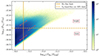 |
Fig. A.1. Correlation between FHα and FY for the redshift bin centred at |

-
transfer of objects across the FHα, lim threshold. Magnified galaxies at the edge of the threshold, with intrinsic luminosity below the survey limit, might be detected and classified as bright or faint, depending on their Y-band flux. This is represented in Fig. A.1 with the two arrows across the continuous line. The transfer between discarded objects and bright and faint populations is parameterised by the slope coefficients sB, Hα and sF, Hα, respectively. These two coefficients are estimated from a version of the bright and faint catalogue with deeper coverage in Hα flux, keeping the YE-band flux selection fixed;
-
transfer of objects across the FYE, lim cut between the faint and bright population. Objects that are intrinsically too faint to be classified as bright and are at the edge of the flux cut, if magnified, may be included in the bright population, and vice versa. This transfer is represented with the arrow across the dashed line and can be parameterised with the slope coefficient sB, YE. This coefficient is estimated from the slope of the cumulative number of bright objects after applying the cut in the Hα flux.
The effective values of the local count slopes can also be estimated directly using the following procedure:
-
We magnify the fluxes by an arbitrary factor
 . For each object, we have
 (A.12)
 -
We repeat our selection, using the magnified fluxes. It is crucial at this point that the flux cut is exactly the same applied to the original fluxes.
-
Denoting with NB/F the number of objects in the bright/faint catalogue selected with the original fluxes, and with
 the number of objects selected with the magnified fluxes, we can estimate the effective local count slope as (Hildebrandt 2016)
 (A.13)
The result does not depend on the value of
 , for small values of
  . Notice that
  is the relative variation in flux that we have applied. Therefore, we are effectively computing numerically the logarithmic derivative of the total number of objects in the bright/faint catalogue with respect to a flux variation, which is the definition of the local count slope.
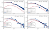 |
Fig. A.2. Angular power spectra for split 1 (50% of bright galaxies and 50% of faint galaxies). Each panel represents a combination of maps: the top-left panel is the cross-correlation of the two number count maps of the bright sample, the top-right panel is the cross-correlation of the faint sample map at low redshift with the bright sample map at high redshift (both sensitive to the local count slope of the bright population), the bottom-left panel is the cross-correlation of the bright sample map at low redshift with the faint sample map at high redshift, and the bottom-right panel is the cross-correlation of the two number count maps of the faint sample (both sensitive to the local count slope of the faint population). Data points represent simulation measurements, using the estimator defined in Eq. (A.14). Continuous red lines show the theory prediction using the analytical formula derived in this section for the local count slope, and black dotted lines are the predictions obtained from the values of the local count slope computed using the numerical differentiation method described in the text. A dashed line shows the absolute value of the theory model obtained with a local count slope equal to zero, that is, assuming no flux magnification (their true values are negative). |
We compared the value of the local count slope using the two methods described above, finding agreement at the level of a few percent. We tested the consistency of both these measurements with the lensing magnification measured in the cross-correlation between redshift bins. As test cases, we considered the split with 50% bright and 50% faint objects (split 1), and the split with 10% bright and 90% faint objects (split 2). We constructed number count maps of the bright and faint populations. The binning in redshift was performed using the background redshift, so that RSD effects are not present. We considered two types of maps: maps that are constructed from the comoving position of the objects and selected based on their intrinsic flux (no flux magnificaton), and maps constructed from the magnified position of the objects and selected based on their magnified flux. The first case includes only contribution from the local density fluctuations of the galaxies, and the second case includes also lensing magnification.
For each split, we estimated the angular cross spectrum by cross-correlating a map at low redshift ( ) with a map at high redshift (
 ). In total, there are four possible configurations: (map of bright galaxies at
  ) × (map of bright galaxies at
  ), (map of faint galaxies at
  ) × (map of bright galaxies at
  ), (map of bright galaxies at
  ) × (map of faint galaxies at
  ), and (map of faint galaxies at
  ) × (map of faint galaxies at
  ). Following Fosalba et al. (2015), we constructed an estimator for the magnified spectra Cℓest, given by
 (A.14)
where Cℓest, magn are the cross spectra estimated from the magnified maps, while Cℓest, dens are extracted from the density maps. The latter spectra are consistent with zero within statistical fluctuations, because there is no overlap between the two redshift bins. Therefore, this estimator removes the sample variance.
In Figs. A.2 and A.3 we compare the cross spectra estimated from the FS data with the two theory predictions for the local count slope that we have described above, for split 1 and split 2, respectively. Continuous red lines use values of the effective local count slope estimated from the analytical formula (theory 1), while black dotted lines represent the theory prediction with local count slope measured from the numerical derivative of the galaxy counts with respect to a variation of flux (theory 2). The theory prediction has been predicted using the CLASS code (Blas et al. 2011; Lesgourgues 2011; Di Dio et al. 2013), using the HMCODE to model nonlinearities (Mead et al. 2016). For comparison, we also show in dashed red lines the absolute value of the theory prediction obtained setting the value of local count slope to zero (their true values are negative). While the latter prediction is completely off compared to the simulation measurements, the other two theory spectra are almost identical and agree very well with the data from FS. This cross-correlation, for all four combinations of maps, is mostly dominated by the cross-correlation of the galaxy density at  (sensitive to the galaxy bias) and lensing magnification at
  (sensitive to the local count slope). Therefore, it shows that the measurements of the local count slope are consistent with the magnification signal in the galaxy clustering angular statistics.
Appendix B: Properties of the galaxy populations
In Table B.1, we report the properties of the galaxy populations we have used in our analysis.
Specifics of the most representative galaxy samples.
All Tables
Impact of satellite galaxies and flux magnification on the detection significance.
All Figures
|
Fig. 1. Dipole model, including the contribution from nonlinear gravitational redshift. The top panel includes linear scales up to 120 h−1 Mpc, while the bottom panel is a zoom-in of the observable on nonlinear scales, up to 30 h−1 Mpc. In the two panels, we use a different range to display the dipole model for better visualization: the dipole amplitude is significantly larger on small scales. Specifics are taken from Table B.1, using the split 90% faint, 10% bright. Top and bottom panels focus on the large-scale and small-scale dipole predictions, respectively. |
| In the text | |
|
Fig. 2. Theory uncertainty, given by the square root of the diagonal elements of the theory covariance, estimated for the redshift bin |
| In the text | |
|
Fig. 3. Correlation of galaxy fluxes with the mass of the host halo. The top panel includes only central galaxies, the bottom panel includes both central and satellite galaxies. The reference fluxes are FHα0 = 1 erg cm−2 s−1 and FY0 = FJ0 = FH0 = 1 erg cm−2 s−1 Hz−1, while the reference halo mass is give by M0 = 1 h−1 M⊙, where M⊙ is the mass of the Sun. The colourbar highlights the density of objects in arbitrary units. |
| In the text | |
|
Fig. 4. Comparison of the uncertainty estimate from the theory covariance (continuous lines) and numerical covariance, computed from the mock using the JK resampling method (data points). We consider the two representative redshift bins centred at |
| In the text | |
|
Fig. 5. S/N of the dipole on linear scales (≥20 h−1 Mpc) for a range of population splits. Here the model prediction is given by linear theory. |
| In the text | |
|
Fig. 6. Measurements of the dipole on small scales, compared to the phenomenological theory model described in Sect. 2.2. The left panels refer to the 50%–50% split, the right panels refer to the 10%–90% split. The rows from top to bottom correspond to the measurements at redshift |
| In the text | |
|
Fig. 7. Measurements of the dipole isolating different contributions, using the 10% bright – 90% faint split. In the left panels, we show the ‘light cone’ data points from the catalogue using the background redshift to perform both selection and measurements, while ‘Doppler + light cone’ uses the redshift corrected by the peculiar velocities of the galaxies. In the right panels, ‘gravitational redshift + light cone’ uses a redshift that includes gravitational redshift but does not account for the peculiar motion of the sources, and the measurements labelled as ‘all’ include both peculiar velocities and gravitational redshift. The theory predictions (red continuous lines) represent our fiducial theory model, which incorporates linear velocities and nonlinear gravitational redshift. Rows from top to bottom correspond to measurements at redshift |
| In the text | |
|
Fig. 8. Impact of satellite galaxies (left panels) and flux magnification (right panels) on the measurements, for the 10% bright – 90% faint split. Since in our fiducial model velocities are treated linearly, flux magnification has a negligible impact on the theory prediction. Rows from top to bottom correspond to measurements at redshift |
| In the text | |
|
Fig. A.1. Correlation between FHα and FY for the redshift bin centred at |
| In the text | |
|
Fig. A.2. Angular power spectra for split 1 (50% of bright galaxies and 50% of faint galaxies). Each panel represents a combination of maps: the top-left panel is the cross-correlation of the two number count maps of the bright sample, the top-right panel is the cross-correlation of the faint sample map at low redshift with the bright sample map at high redshift (both sensitive to the local count slope of the bright population), the bottom-left panel is the cross-correlation of the bright sample map at low redshift with the faint sample map at high redshift, and the bottom-right panel is the cross-correlation of the two number count maps of the faint sample (both sensitive to the local count slope of the faint population). Data points represent simulation measurements, using the estimator defined in Eq. (A.14). Continuous red lines show the theory prediction using the analytical formula derived in this section for the local count slope, and black dotted lines are the predictions obtained from the values of the local count slope computed using the numerical differentiation method described in the text. A dashed line shows the absolute value of the theory model obtained with a local count slope equal to zero, that is, assuming no flux magnification (their true values are negative). |
| In the text | |
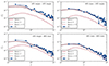 |
Fig. A.3. Same as in Fig. A.2, but for split 2 (10% of bright galaxies and 90% of faint galaxies). |
| In the text | |
Current usage metrics show cumulative count of Article Views (full-text article views including HTML views, PDF and ePub downloads, according to the available data) and Abstracts Views on Vision4Press platform.
Data correspond to usage on the plateform after 2015. The current usage metrics is available 48-96 hours after online publication and is updated daily on week days.
Initial download of the metrics may take a while.