| Issue |
A&A
Volume 695, March 2025
|
|
|---|---|---|
| Article Number | A262 | |
| Number of page(s) | 15 | |
| Section | Numerical methods and codes | |
| DOI | https://doi.org/10.1051/0004-6361/202452351 | |
| Published online | 26 March 2025 | |
Time-adaptive PIROCK method with error control for multi-fluid and single-fluid magnetohydrodynamics systems
1
Lockheed Martin Solar & Astrophysics Laboratory,
3251 Hanover St,
Palo Alto,
CA
94304,
USA
2
Bay Area Environmental Research Institute,
NASA Research Park,
Moffett Field,
CA
94035,
USA
3
Section of Mathematics, University of Geneva,
Switzerland
4
Rosseland Centre for Solar Physics, University of Oslo,
PO Box 1029 Blindern,
0315
Oslo,
Norway
5
Institute of Theoretical Astrophysics, University of Oslo,
PO Box 1029 Blindern,
0315
Oslo,
Norway
6
SETI Institute,
339 Bernardo Ave
Mountain View,
CA
94035,
USA
★ Corresponding author
Received:
23
September
2024
Accepted:
6
February
2025
Context. The solar atmosphere is a complex environment characterized by numerous species with varying ionization states, which are particularly evident in the chromosphere, where the significant variations in ionization degree occur. This region transitions from highly collisional to weakly collisional states that exhibit diverse plasma state transitions influenced by varying magnetic strengths and collisional properties. The complexity of processes in the solar atmosphere introduces substantial numerical stiffness in multi-fluid models, leading to severe timestep restrictions in standard time integration methods.
Aims. To address the computational challenges, new numerical methods are essential. These methods must effectively manage the diverse timescales associated with multi-fluid and multi-physics models, including convection, dissipative effects, and reactions. The widely used time operator splitting technique provides a straightforward approach but necessitates careful timestep management to prevent stability issues and errors. Despite studies on splitting errors, their impact on solar and stellar astrophysics has largely been overlooked.
Methods. We focus on a multi-fluid multi-species model, which poses significant challenges for time integration. We propose a second-order Partitioned Implicit-Explicit Orthogonal Runge–Kutta (PIROCK) method. This method combines efficient explicit stabilized and implicit integration techniques while employing variable time-stepping with error control.
Results. Compared to a standard third-order explicit time integration method and a first-order Lie splitting approach as considered recently, the PIROCK method demonstrates robust advantages in terms of accuracy, numerical stability, and computational efficiency. For the first time, our results reveal PIROCK’s capability to effectively solve multi-fluid problems with unprecedented efficiency. Preliminary results on chemical fractionation, combined with this efficient method, represent a significant step toward understanding the well-known first-ionization-potential effect in the solar atmosphere.
Key words: magnetic reconnection / magnetohydrodynamics (MHD) / plasmas / shock waves / waves / Sun: chromosphere
© The Authors 2025
 Open Access article, published by EDP Sciences, under the terms of the Creative Commons Attribution License (https://creativecommons.org/licenses/by/4.0), which permits unrestricted use, distribution, and reproduction in any medium, provided the original work is properly cited.
This article is published in open access under the Subscribe to Open model. Subscribe to A&A to support open access publication.
1 Introduction
The solar atmosphere which is characterized by complexity, houses numerous species with varying ionization states. This complexity is most obvious in the solar chromosphere, which exhibits significant variations in ionization degree, transitioning from highly collisional to weakly collisional states. In particular, the chromosphere exhibits various plasma state transitions, showcasing diverse magnetic strengths and collisional properties across different regions (see Morosin et al. 2022; Przybylski et al. 2022; Martínez-Sykora et al. 2020; Ni et al. 2020). The growing awareness of the significance of ion-neutral interactions in influencing the dynamics and energy balance of the lower solar atmosphere is evident within the scientific community, in the codes that have been developed, and in ongoing efforts (see Martínez-Sykora et al. 2015; Ballester et al. 2018; Soler & Ballester 2022, and references therein).
When constructing multi-fluid models, the complex nature of processes in the solar atmosphere introduces significant numerical stiffness, leading to severe timestep restrictions based on standard time integration methods. To mitigate computational costs, new numerical methods are required. Attention must be given to the numerical method’s capability to handle the diverse timescales associated with multi-fluid and multi-physics models, including convection, dissipative effects, reactions, and other processes. Alvarez Laguna et al. (2016) employed a numerical strategy based on a full implicit integration to address the numerical stiffness inherent in the multi-fluid magnetohydrodynamics (MHD) equations. However, implicit approaches demand substantial memory resources and involve expensive linear algebra tools. As an alternative, researchers commonly employ conventional explicit schemes, such as Runge–Kutta (RK) methods (e.g. the fourth-order RK scheme by Vögler et al. 2005; Navarro et al. 2022; Wray et al. 2015). Another notable technique is the third-order 2 N RK scheme (RK3-2N) introduced by Carpenter & Kennedy (1994) and explored by Gudiksen et al. (2011) and Brandenburg et al. (2021) among others. Despite their ease of implementation, these methods often face challenges in efficiently handling the time integration of stiff equations. The stiffness is primarily attributed to the stringent Courant-Friedrichs-Lewy (CFL) condition they impose, and thus they require small timesteps for stability. The impact of this limitation becomes particularly evident in the context of the multi-fluid MHD model (see Wargnier et al. 2023; Leake et al. 2012; Jara-Almonte et al. 2021).
In the field of solar physics, a notable challenge revolves around integrating (in time) diffusive terms such as the thermal conduction of electrons and the ambipolar diffusion coefficient. Specifically, codes such as MANCHA3D (Navarro et al. 2022) and MURAM (Vögler et al. 2005; Rempel 2017; Przybylski et al. 2022) confront this challenge by adopting a parabolic-hyperbolic approach for thermal conduction. This method involves solving a non-Fickian diffusion equation, as elaborated by Rempel (2017). An alternative strategy, the super-time-stepping (STS) method (Genevi et al. 1996), has been widely employed, such as in González-Morales et al. (2018) and Nóbrega-Siverio et al. (2020a), to address ambipolar diffusion and to address the thermal conduction (e.g., Navarro et al. 2022). With construction based on Chebyshev polynomials, this STS method can be easily implemented explicitly and allows for a relaxed CFL condition and larger timesteps. However, the main drawback of the STS method is not only its first-order accuracy but also its internal stability issues concerning round-off errors. In the numerical analysis literature, this stability issue was already analyzed in van der Houwen & Sommeijer (1980), and an implementation, named the Runge–Kutta–Chebyshev (RKC) method, based on recurrence relations with favorable internal stability has been proposed. In Meyer et al. (2012),1 the Runge–Kutta–Legendre STS method, a second-order variant of the second-order RKC method from van der Houwen & Sommeijer (1980) was proposed based on the family of Legendre polynomials with the main feature of higher damping properties in the stabilization of diffusion terms in the context of astrophysical MHD simulations. Attention was then directed towards the explicit second-order orthogonal Chebyshev method known as ROCK2 (Abdulle & Li 2008; Abdulle 2002; Abdulle & Medovikov 2001; Zbinden 2011). Although not yet applied in the context of solar physics simulations, the ROCK2 method demonstrates competitiveness with implicit solvers and offers adaptive stability domains tailored to challenging dissipative problems taking advantage of high damping properties of near optimal families of orthogonal polynomials.
Effectively addressing the simultaneous treatment of convective-diffusive-source terms in a multi-fluid MHD model, which is akin to solving a conventional stiff reaction-convective-diffusion problem, poses a notable challenge in developing a temporal integration method. The commonly used time operator splitting technique, as explored in Strang (1968); Duarte et al. (2012); Duarte (2011); Descombes et al. (2014), offers a straightforward approach to separately integrating these terms. As noted already in Meyer et al. (2012, Sect. 3.3), explicit stabilized methods may suffer from stability issues when applied also to hyperbolic terms and are typically applied in astrophysical MHD simulations only to the diffusion terms in combination with splitting methods where the parabolic and non-parabolic terms are integrated alternatively (see the recent literature in Caplan et al. 2024; Shoda et al. 2024; Zhou et al. 2024). Such explicit stabilized methods, which are widely employed in solar physics and have been seen in applications such as Bifrost (Gudiksen et al. 2011), are suitable for the multi-fluid MHD model through a splitting strategy. Careful management of the timestep is crucial due to potential errors from splitting, which can globally impact the overall temporal accuracy. This holds even when accurate temporal integration methods of high order are considered separately. Attempts to comprehend these errors have been undertaken within applied mathematics, particularly in studies by Descombes et al. (2011) and Descombes et al. (2014).
An alternative strategy involves partitioned implicit-explicit Runge–Kutta methods (IRKC), as proposed by Verwer & Sommeijer (2004). Additionally, a second-order partitioned method, PRKC, is discussed by Zbinden (2011) combining a second-order explicit stabilized method with a third-order explicit Runge–Kutta method. In this work, we have considered the PIROCK method developed by Abdulle & Vilmart (2013a), a partitioned Runge–Kutta method inspired by the earlier approaches (Abdulle 2002; Verwer & Sommeijer 2004; Zbinden 2011) and combining efficient integration methods, precisely ROCK2 for diffusive terms, a third-order Runge–Kutta Heun method, and a second-order Singly Diagonally Implicit Runge–Kutta (SDIRK) method for reactive terms. The method incorporates an adaptive timestep strategy using local error estimators based on embedded methods.
We consider a comprehensive multi-fluid multi-species (MFMS) model detailed in our prior work Wargnier et al. (2023), addressing a convective–diffusive–reaction problem with the inclusion of the Hall term. In Section 2, we provide a brief overview of the model within the context of a single ordinary differential equation. Following that, we detail the spatial discretization and the formulation of hyperdiffusive terms incorporated into the model in Section 3. Moving on to Section 4, we review methods found in the literature for separately integrating diffusive, advective, and stiff reactive terms, using a simple Dahlquist test problem as a reference. We also discuss the time integration strategy employed in the solar physics literature for integrating these terms collectively. In Section 5, we provide a brief description of the PIROCK algorithm, its modification, and the adaptive timestep control strategy based on error estimators. In Section 6, we present and compare simulation results using PIROCK against third-order explicit time integration and a first-order Lie splitting method (e.g., Wargnier et al. 2023). We aim to demonstrate PIROCK as the optimal strategy for MFMS model time integration, significantly reducing computational costs while maintaining second-order accuracy. We highlight its efficiency compared to classical explicit methods, such as the Bifrost code for single-fluid MHD models, including hyperdiffusive terms and ambipolar diffusion.
2 Multi-fluid multi-species governing equations
This section provides an overview of the Multi-fluid Multi-Species (MFMS) model. The model was previously described in Section 2 of Wargnier et al. (2023), where additional details were provided. In subsequent discourse, the notation i shall represent a fluid of species associated with a heavy particle at any ionization level or excited state, excluding electrons, within the composite mixture of electrons and heavy particles. The notation e represents the electron fluid.
In contrast to previous work (Wargnier et al. 2023), we account for all terms without any simplifications, including the Hall term. After discretization in space, the system of equations can be straightforwardly reformulated as a set of ordinary differential equations that are segregated into different terms as depicted by the equation:
![$\[\frac{d \mathbf{Y}(t)}{d t}=\mathbf{F}_{\mathrm{A}}(\mathbf{Y}(t))+\mathbf{F}_{\mathrm{R}}(\mathbf{Y}(t))+\mathbf{F}_{\mathrm{D}}(\mathbf{Y}(t)),\]$](/articles/aa/full_html/2025/03/aa52351-24/aa52351-24-eq1.png) (1)
(1)
where ![$\[\mathbf{Y}=\left(\rho_{i}, \rho_{i} \mathbf{u}_{i}^{T}, e_{i}, e_{\mathrm{e}}, \mathbf{B}^{T}\right)^{T}\]$](/articles/aa/full_html/2025/03/aa52351-24/aa52351-24-eq2.png) is the vector of conservative variables that involves the mass density ρi, velocity ui, thermal energies ei of each ionized/excited or ground level heavy species, as well as the electron thermal energy e𝔢 and the magnetic field B. FA, FD, and FR are the advective, diffusive fluxes and reactive terms, respectively, and are defined in a compact form as follows:
is the vector of conservative variables that involves the mass density ρi, velocity ui, thermal energies ei of each ionized/excited or ground level heavy species, as well as the electron thermal energy e𝔢 and the magnetic field B. FA, FD, and FR are the advective, diffusive fluxes and reactive terms, respectively, and are defined in a compact form as follows:
![$\[\left\{\begin{aligned}\mathbf{F}_{\mathrm{A}}(\mathbf{Y}) & =-\nabla \cdot \mathbf{f}_{\mathrm{A}}(\mathbf{Y})-\mathbf{S}_{\mathrm{A}}(\mathbf{Y}, \nabla \mathbf{Y}), \\\mathbf{f}_{\mathrm{A}}(\mathbf{Y}) & =\left(\rho_i \mathbf{u}_i, \rho_i \mathbf{u}_i \otimes \mathbf{u}_i+P_i \mathbb{I}, e_i \mathbf{u}_i, e_{\mathrm{e}} \mathbf{u}_{\mathrm{e}}, \mathbb{I} \wedge\left(\mathbf{u}_{\mathrm{e}} \wedge \mathbf{B}\right)\right)^T, \\\mathbf{S}_{\mathrm{A}}(\mathbf{Y}, \nabla \mathbf{Y}) & =\left(0_i, n_i q_i\left(\left[\mathbf{u}_{\mathrm{e}}-\mathbf{u}_i\right] \wedge \mathbf{B}-\frac{\nabla P_{\mathrm{e}}}{n_{\mathrm{e}} q_{\mathrm{e}}}\right),\right. \\& \left.P_i \nabla \cdot \mathbf{u}_i, P_{\mathrm{e}} \nabla \cdot \mathbf{u}_{\mathrm{e}},-\nabla \wedge\left(\frac{\nabla P_{\mathrm{e}}}{n_{\mathrm{e}} q_{\mathrm{e}}}\right)\right)^T\end{aligned}\right.\]$](/articles/aa/full_html/2025/03/aa52351-24/aa52351-24-eq3.png) (2)
(2)
![$\[\begin{aligned}& \left\{\begin{array}{l}\mathbf{F}_{\mathrm{D}}(\mathbf{Y})=\nabla \cdot \mathbf{f}_{\mathrm{D}}(\nabla \mathbf{Y}) \\\mathbf{f}_{\mathrm{D}}(\nabla \mathbf{Y})=\left(0_i, \boldsymbol{\tau}_i^*,-\boldsymbol{\tau}_i^*: \nabla \mathbf{u}_i, H_{\mathrm{e}}^{\text {spitz }}, \mathbb{I} \wedge\left(\frac{\mathbf{R}_{\mathrm{e}}^\text{col}}{n_{\mathrm{e}} q_{\mathrm{e}}}+\mathbf{E}^*\right)\right)^T\end{array}\right. \\& \left\{\begin{array}{l}\mathbf{F}_{\mathrm{R}}(\mathbf{Y})=\left(\Gamma_i^{\text {ion,rec }}, \mathbf{R}_i^{\text {ion,rec }}+\mathbf{R}_i^{\mathrm{col}}+\left[\frac{n_i q_i}{n_{\mathrm{e}} q_{\mathrm{e}}}\right] \mathbf{R}_{\mathrm{e}}^{\mathrm{col}},\right. \\\left.H_i^{\text {ion,rec }}+H_i^{\text {col }}, H_{\mathrm{e}}^{\text {ion,rec }}+H_{\mathrm{e}}^{\mathrm{col}}, 0_3\right)^T\end{array}\right.\end{aligned}\]$](/articles/aa/full_html/2025/03/aa52351-24/aa52351-24-eq4.png) (3)
(3)
where Pi and P𝔢 denote the pressure of a particular fluid species i, and the electron pressure respectively. 𝕀 is the identity matrix, 03 is the null matrices of size three, ni and n𝔢 are the number densities of particular fluid species i and electrons respectively, while qi and q𝔢 are the ion and electron charges, respectively.
The advective terms FA are split into advective fluxes ∇ · fA(Y) and source terms SAY, ∇Y). In contrast to the reactive terms FR discussed later, the advection source terms SA have the particularity of depending on the gradient of the conservative variables ∇Y, rendering them less suitable for integration with an implicit method, as considered for FR. Furthermore, SA includes non-conservative products such as Pi∇ · ui or P𝔢∇ · u𝔢. The source term SA includes also the battery term ∇ P𝔢/(n𝔢q𝔢) and the ion-coupling term niqi ([u𝔢 − ui] ∧ B). In our study, we have also treated the ion-coupling term as a reactive source term FR, assuming a constant magnetic field and current during its integration. This strategy is convenient in cases where the term becomes numerically stiff. Our results, which demonstrate satisfactory performance in calculations and accuracy, support the feasibility of this approach.
The diffusive fluxes FD encompass physical diffusive terms, such as ![$\[H_{\mathrm{e}}^{\text {spitz }}\]$](/articles/aa/full_html/2025/03/aa52351-24/aa52351-24-eq5.png) representing the anisotropic electron heat flux, and
representing the anisotropic electron heat flux, and ![$\[\mathbf{R}_{\mathrm{e}}^{\mathrm{col}} /\left(n_{\mathrm{e}} q_{\mathrm{e}}\right)\]$](/articles/aa/full_html/2025/03/aa52351-24/aa52351-24-eq6.png) , which denotes the collision term derived from the electron momentum equation and is defined within the electric field formulation. Additionally, artificial hyperdiffusive terms such as
, which denotes the collision term derived from the electron momentum equation and is defined within the electric field formulation. Additionally, artificial hyperdiffusive terms such as ![$\[\boldsymbol{\tau}_{i}^{*}\]$](/articles/aa/full_html/2025/03/aa52351-24/aa52351-24-eq7.png) and E* for each momentum equation associated with species i and magnetic field are included. Further elaboration on the hyperdiffusive terms in the MFMS context is provided in the subsequent Section 3. The diffusive term, being the divergence of a function dependent on the gradient of the conservative variable, behaves akin to a second-order differential operator.
and E* for each momentum equation associated with species i and magnetic field are included. Further elaboration on the hyperdiffusive terms in the MFMS context is provided in the subsequent Section 3. The diffusive term, being the divergence of a function dependent on the gradient of the conservative variable, behaves akin to a second-order differential operator.
In the definition of the reactive terms ![$\[\mathbf{F}_{\mathrm{R}}, \Gamma_{i}^{\text {ion,rec }}\]$](/articles/aa/full_html/2025/03/aa52351-24/aa52351-24-eq8.png) is the sum of the mass transition rate due to recombination or de-excitation, and ionization or excitation, associated with fluid species i.
is the sum of the mass transition rate due to recombination or de-excitation, and ionization or excitation, associated with fluid species i. ![$\[\mathbf{R}_{i}^{\text {ion,rec }}\]$](/articles/aa/full_html/2025/03/aa52351-24/aa52351-24-eq9.png) is sum of all the momentum exchange terms for species i due to both ionization and recombination processes.
is sum of all the momentum exchange terms for species i due to both ionization and recombination processes. ![$\[H_{i}^{\text {ion,rec }}\]$](/articles/aa/full_html/2025/03/aa52351-24/aa52351-24-eq10.png) and
and ![$\[H_{\mathrm{e}}^{\text {ion,rec }}\]$](/articles/aa/full_html/2025/03/aa52351-24/aa52351-24-eq11.png) are the sum of the heating and cooling terms due to the ionization and recombination processes associated with particles i and electrons, respectively.
are the sum of the heating and cooling terms due to the ionization and recombination processes associated with particles i and electrons, respectively. ![$\[\mathbf{R}_{i}^{\text {col }}\]$](/articles/aa/full_html/2025/03/aa52351-24/aa52351-24-eq12.png) is the sum of all the momentum exchange terms due to collisions between fluid species i with any other fluid species in the mixture considered,
is the sum of all the momentum exchange terms due to collisions between fluid species i with any other fluid species in the mixture considered, ![$\[H_{i}^{\text {col }}\]$](/articles/aa/full_html/2025/03/aa52351-24/aa52351-24-eq13.png) is the sum of all the heating terms due to collisions associated with particle i. Similarly, as in Wargnier et al. (2023), the radiative losses are optically thin in the term
is the sum of all the heating terms due to collisions associated with particle i. Similarly, as in Wargnier et al. (2023), the radiative losses are optically thin in the term ![$\[H_{\mathrm{e}}^{\text {ion,rec }}\]$](/articles/aa/full_html/2025/03/aa52351-24/aa52351-24-eq14.png) . Unlike advective or diffusive terms, these reactive terms lack spatial connectivity. Their numerical stiffness arises from their association with small timescales, such as collisions, ionization, and recombination processes.
. Unlike advective or diffusive terms, these reactive terms lack spatial connectivity. Their numerical stiffness arises from their association with small timescales, such as collisions, ionization, and recombination processes.
Given the quasi-neutrality assumption and the presence of multiple ionized species, the electron velocity can be expressed as a function of the hydrodynamic velocity of each ion and the total current. This is written as:
![$\[\mathbf{u}_{\mathrm{e}}=\sum_i \frac{n_i q_i \mathbf{u}_i}{n_{\mathrm{e}} q_{\mathrm{e}}}-\frac{\mathbf{J}}{n_{\mathrm{e}} q_{\mathrm{e}}},\]$](/articles/aa/full_html/2025/03/aa52351-24/aa52351-24-eq15.png) (4)
(4)
where J = (∇ ∧)/μ0 is the total current defined from Maxwell-Ampere’s law and μ0 is the vacuum permeability. We note that the Hall term appears in the magnetic induction in fA by considering the contribution of the total current of the electron velocity in the second term of Eq. (4).
3 Spatial discretization and hyper-diffusive terms treated as FD
We emphasize that this paper mainly focuses on temporal integration while the considered spatial discretization method utilized in this study closely resembles the approach outlined by Gudiksen et al. (2011), as detailed in the previous work Wargnier et al. (2023). It entails the application of a sixth-order differential operator for calculating gradients associated with convective and diffusive fluxes, along with a fifth-order interpolation scheme for repositioning conservative quantities on a staggered grid. We highlight that the method presented here is general and could be adapted straightforwardly to other choices of spatial discretization methods. After spatial discretization, it treats temporal integration as an ordinary differential equation, as depicted in Eq. (1).
The high-order finite difference scheme necessitates the incorporation of artificial numerical terms, referred to as hyperdiffusive terms. Analogous to Nordlund (1982) in the single-fluid MHD case, these terms are employed for stability and mitigate spurious oscillations near shocks or discontinuities, also known as the Gibbs phenomenon. The initial MFMS model is adjusted for numerical approximation needs by including artificial hyperdiffusive terms to enhance stability. It is important to note that these terms are treated as diffusive terms (FD). They will be temporarily integrated using the same method employed for physical diffusive terms, such as electron thermal conduction.
The hyperdiffusive terms are defined by ![$\[\boldsymbol{\tau}_{i}^{*}\]$](/articles/aa/full_html/2025/03/aa52351-24/aa52351-24-eq16.png) and E* in fD. The artificial viscous stress tensor for each momentum equation is defined in a parabolic form for any fluid-species i, as follows:
and E* in fD. The artificial viscous stress tensor for each momentum equation is defined in a parabolic form for any fluid-species i, as follows:
![$\[\nabla \cdot \boldsymbol{\tau}_i^*=\nabla \cdot\left(\alpha_i\left(\mathbf{u}_i\right) \nabla\left(\mathbf{u}_i\right)\right)\]$](/articles/aa/full_html/2025/03/aa52351-24/aa52351-24-eq17.png) (5)
(5)
![$\[\alpha_i\left(\mathbf{u}_i\right)=\left(C_i^k ~\Delta k ~Q\left(\partial_k \text{u}_{i, j}\right)\right)_{k, j \in\{x, y, z\}^2},\]$](/articles/aa/full_html/2025/03/aa52351-24/aa52351-24-eq18.png) (6)
(6)
where Δk denotes the grid spacing sizes along dimensions x, y, or z; Q defined by Gudiksen et al. (2011) functions as a quenching operator aimed at detecting strong gradients or discontinuities in space and amplifying diffusion within those regions; ∂kui,j denotes the spatial derivative of the j-component of velocity ui along dimension k; and ![$\[C_{i}^{k}\]$](/articles/aa/full_html/2025/03/aa52351-24/aa52351-24-eq19.png) is a factor defined as:
is a factor defined as:
![$\[C_i^k=\rho_i\left(\nu_1 c_{i, f}+\nu_2\left|\mathbf{u}_{i, k}\right|+\nu_3 \Delta k\left|\partial_k \mathbf{u}_{i, k}\right|\right),\]$](/articles/aa/full_html/2025/03/aa52351-24/aa52351-24-eq20.png) (7)
(7)
where ν1, ν2, and ν3 are arbitrary coefficients typically ranging between zero and one; and ci,f is the fast magnetosonic wave associated with species i.
Our study incorporates artificial hyperdiffusive terms into the magnetic field equation represented by E*. This approach mirrors that of Nordlund (1982) for single-fluid MHD but has been extended to MFMS, analogous to the treatment of the viscous stress tensor discussed previously. We introduce supplementary artificial hyperdiffusive terms characterized by timescales corresponding to the Hall and ion-coupling terms, which are absent in the conventional single-fluid MHD framework. Additional elucidation regarding these adjustments aligns with the methodology outlined by Nóbrega-Siverio et al. (2020b) within the framework of the ambipolar diffusion term.
4 Stability of Runge–Kutta methods
The MFMS model Eq. (1) has been explicitly formulated as a sum of three types of terms: diffusion terms (FD), advection terms (FA), and stiff reactive terms (FR). Both types of terms FD and FA display spatial connectivity, whereas the stiff source terms (FR) lack spatial connectivity and feature timescales considerably smaller than those associated with other terms.
In this section, following Hairer & Wanner (1996, Section IV), we concentrate on the Dalquist test problem to discuss the time integration of these three types of terms. We review temporal integration methods, predominantly Runge–Kutta methods, emphasizing current effective and accurate approaches.
4.1 The Dalquist equation
We considered the so-called Dahlquist test equation
![$\[\frac{d y(t)}{d t}=F(y(t))=\lambda y(t), y(0)=1,\]$](/articles/aa/full_html/2025/03/aa52351-24/aa52351-24-eq21.png) (8)
(8)
where λ ∈ ℂ is a fixed parameter corresponding to an eigenvalue of the system obtained after linearizing a nonlinear stiff system of differential equations. It is well understood that in the considered Eq. (1), the function F from Eq. (8) plays the role of the respective terms FA, FR, or FD. In this context, for these three cases, the eigenvalue λ will exhibit different characteristics, such as being purely imaginary (FA), complex with a dominant negative real part (FD), or purely real (FR).
Applying to Eq. (8) a Runge–Kutta method with timestep Δt yields a recursion of the form
![$\[y_{n+1}=R(z) y_n,\]$](/articles/aa/full_html/2025/03/aa52351-24/aa52351-24-eq22.png) (9)
(9)
where z = λΔt and R(z) is a rational function called the stability function of the Runge–Kutta method. The numerical solution yn in Eq. (9) remains bounded for n → +∞ if and only if z ∈ S, where we defined the stability domain of the Runge–Kutta method as
![$\[S=\{z \in \mathbb{C};|R(z)| \leq 1\}.\]$](/articles/aa/full_html/2025/03/aa52351-24/aa52351-24-eq23.png) (10)
(10)
Depending on the nature of an evolution problem (FA, FR, or FD), different Runge–Kutta methods can be more suitable. We will review them in the following subsections.
4.2 Explicit stabilized Runge–Kutta methods for diffusion problems
We first focus on diffusive terms applied to the Dahlquist test in Eq. (8) with F = FD. The eigenvalue λ is close to the negative real axis in the complex plane. Tackling the integration of diffusion operators presents challenges due to the numerical stiffness induced by the CFL condition stemming from the involvement of second-order differential operators.
For the explicit Euler method yn+1 = yn + ΔtF(yn), the stability function R(z) = 1 + z defines a stability domain S as a disk centered at −1 with radius 1, encompassing the real interval [−2, 0]. This results in a stability condition Δt ≤ 2/|λ|, where λ denotes the largest eigenvalue. When diffusive terms are discretized using standard finite difference methods with a spatial mesh size Δx, the largest eigenvalue typically scales as |λ| ≤ CΔx−2. This imposes a severe CFL condition to ensure numerical stability.
A natural approach to circumvent this timestep restriction and stability for diffusion problems is to use implicit methods, but these can suffer from a prohibitive cost and difficulties in implementation due to the need for sophisticated linear algebra solvers with preconditioners in Newton-type nonlinear solvers (Hairer & Wanner 1996).
4.2.1 Limitations of the super-time-stepping method
As an alternative to implicit schemes, the use of explicit stabilized methods can be very efficient for diffusion problems, as presented in Hairer & Wanner (1996, Section IV.2) (see also the review by Abdulle (2015)). The idea is to consider explicit schemes with stability function defined in Eq. (9) that have extended stability domains S along the negative real axis as defined in Eq. (10). To achieve such improved stability properties, the main idea is to allow the variation of the number s of the internal stage of the methods that then grow adaptively with the required stability. This is in contrast with standard Runge–Kutta methods, where the number of internal stages is, in general, constant and has to be increased to improve the order of accuracy. For a fixed s ≥ 1, among all polynomials Rs(z) = 1 + z + a2z2 + a3z3 + . . . + aszs of degree at most s, corresponding to consistent explicit s-stage Runge–Kutta methods, the polynomial that maximizes the length Ls of the stability domain [−Ls, 0] ⊂ S is given by
![$\[R_s(z)=T_s\left(1+\frac{z}{s^2}\right)\]$](/articles/aa/full_html/2025/03/aa52351-24/aa52351-24-eq24.png) (11)
(11)
and benefits from the large stability domain size Ls = 2s2 along the negative real axis and Ts denotes the Chebyshev polynomial of degree s (for instance T0(x) = 1, T1(x) = x, T2(x) = 2x2 − 1, . . .). This is shown using the property Ts(cos θ) = cos(sθ) for all θ that characterizes Chebyshev polynomials. This method relaxes the CFL condition of diffusion problems and allows for larger timesteps. It entails an increase in internal stages, resulting in a quadratically expanding the size Ls of the stability domain along the negative real axis, rendering it more stable than standard explicit methods, computationally cheaper and easier to implement than implicit methods. Precisely, the stability condition becomes for diffusion problems Δt|λ| ≤ Ls = 2s2 which yields the relaxed CFL condition Δt ≤ Cs2Δx2.
Then, a naive implementation is to implement such explicit stabilized methods as a composition of explicit Euler steps, as proposed independently by Saul’ev (1960) and Guillou & Lago (1960),
![$\[k_j=k_{j-1}+\delta_j \Delta t F\left(k_{j-1}\right), \quad j=1, \ldots, s,\]$](/articles/aa/full_html/2025/03/aa52351-24/aa52351-24-eq25.png) (12)
(12)
with k0 = yn, and the output yn+1 = ks coincides with the last internal stage, corresponding to the factorization ![$\[R_{s}(z)={\prod}_{j=1}^{s}\left(1+\delta_{j} z\right)\]$](/articles/aa/full_html/2025/03/aa52351-24/aa52351-24-eq26.png) , where −1/δj, j = 1 . . ., s denote the s roots of the optimal stability polynomial Rs defined in Eq. (11) (i.e., Rs(−1/δj) = 0 for all j = 1 . . ., s, see again the review by Abdulle 2015). While the ordering of the roots can be optimized, this naive approach still results in first-order methods with unstable internal stages. As a result, these methods are typically practical only for small degrees s, generally less than ten. This approach was rediscovered as the STS method (see Genevi et al. 1996) and commonly used in the context of the temporal integration of the ambipolar diffusion in single-fluid MHD models by (e.g., Genevi et al. 1996; González-Morales et al. 2018; Nóbrega-Siverio et al. 2020a; Mignone et al. 2007).
, where −1/δj, j = 1 . . ., s denote the s roots of the optimal stability polynomial Rs defined in Eq. (11) (i.e., Rs(−1/δj) = 0 for all j = 1 . . ., s, see again the review by Abdulle 2015). While the ordering of the roots can be optimized, this naive approach still results in first-order methods with unstable internal stages. As a result, these methods are typically practical only for small degrees s, generally less than ten. This approach was rediscovered as the STS method (see Genevi et al. 1996) and commonly used in the context of the temporal integration of the ambipolar diffusion in single-fluid MHD models by (e.g., Genevi et al. 1996; González-Morales et al. 2018; Nóbrega-Siverio et al. 2020a; Mignone et al. 2007).
4.2.2 Second-order orthogonal Chebyshev method
The stability issues related to round-off errors, primarily due to instabilities in the internal stages, were effectively addressed in the seminal work by van der Houwen & Sommeijer (1980). They resolved this by computing the internal steps of the Runge–Kutta methods using a recurrence formula analogous to the recurrence formula Tj(x) = 2xTj−1(x) − Tj−2(x) for all j ≥ 2 of Chebyshev polynomials. The internal steps are then given by:
![$\[k_j=\frac{2 \Delta t}{s^2} F\left(k_{j-1}\right)+2 k_{j-1}-k_{j-2}, \quad j=2, \ldots, s,\]$](/articles/aa/full_html/2025/03/aa52351-24/aa52351-24-eq27.png) (13)
(13)
where ![$\[k_{0}=y_{n}, k_{1}=y_{n}+\frac{\Delta t}{s^{2}} F\left(y_{n}\right)\]$](/articles/aa/full_html/2025/03/aa52351-24/aa52351-24-eq28.png) , and the output yn+1 = ks coincides with the last internal stage.
, and the output yn+1 = ks coincides with the last internal stage.
Although both implementations in Eqs. (12) and (13) share the same stability function (Eq. (11)), making them equivalent methods for a linear vector field F and in the absence of roundoff errors, the advantage of the implementation in Eq. (13) based on the Chebyshev recurrence compared with the STS method in Eq. (12) is illustrated in Fig. 1. Here, favorable internal stability is observed compared to the naive implementation in Eq. (12), where the stability polynomials of the internal stages exhibit large amplitude oscillations. This issue is evident for s = 10 and worsens as the number of internal stages s increases, making Eq. (12) unusable for larger numbers s of stages due to its unstable behavior already with respect to roundoff errors, as analyzed by van der Houwen & Sommeijer (1980).
In particular, the main contribution in van der Houwen & Sommeijer (1980) is a class of second-order explicit stabilized methods based on Chebyshev polynomials with favorable internal stability and error control, known as the RKC method. This work inspired new classes of explicit stabilized methods with quasi-optimally large stability domains, notably the explicit second-order orthogonal Chebyshev method known as ROCK2 based on appropriate families of orthogonal polynomials2 (Abdulle & Li 2008; Abdulle 2002; Abdulle & Medovikov 2001; Zbinden 2011).
The ROCK2 method shares a concept similar to the STS method, featuring a quadratically increasing stability domain, but boasts three significant advantages. Firstly, STS is only first order, while ROCK2 is a second-order method with a stability condition Δt|λ| ≤ Cs2, where C = 0.81 is quasi-optimal among second-order explicit stabilized methods (see the stability domain as defined in Eq. (10) of length L13 ≃ 136 in the left picture of Fig. 2). Secondly, ROCK2 can handle large internal stages (up to 200 is implemented) without encountering stability issues, thanks to a recurrence based on orthogonal polynomials, compared to the ten-stage limit for STS. Lastly, ROCK2 includes an embedded method, enabling seamless integration with an error estimator for optimal timestep estimation, as detailed in Section 5.2. We note that the hyperdiffusive term can be implemented and benefit from this method. Notably, it does not require a precise spectral radius estimation but only an upper bound, providing a significant computational cost advantage. Further details can be found in Appendix A.
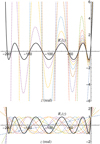 |
Fig. 1 Comparison of the STS implementation in Eq. (12), top, and the stable implementation based on Chebyshev recurrence in Eq. (13), bottom, of the first-order Chebyshev method with an optimal stability polynomial given in Eq. (11). The stability polynomial Rs(z) defined in Eq. (11) for s = 10 (see black curves) and the stability polynomials of internal stages (related to kj, j = 1 . . ., s − 1, see color curves) are plotted as a function of z which is assumed purely real here. The STS implementation exhibits poor internal stability, with internal stability polynomials oscillating with large amplitude resulting in instabilities with respect to roundoff errors, in contrast to the Chebyshev recurrence implementation defined in Eq. (13), with favorable internal stability where the amplitude of the internal stage stability polynomials remains bounded by 1. |
 |
Fig. 2 Stability domains as defined in Eq. (10) of the schemes involved in PIROCK: ROCK2 (in gray. here s = 13 internal stages) for diffusion terms, an explicit method of order 3 for advection terms (dark gray), and the L-stable diagonally implicit Runge–Kutta method of order 2 for stiff reaction terms (light gray). Right picture: Zoom near the origin to illustrate that the advection method (dark gray) includes the portion of the imaginary axis. The stability domains are plotted for z in the complex plane (horizontal axis: real part Re(z), vertical axis: imaginary part Im(z)). |
4.3 Runge–Kutta methods for advection problems and diagonally implicit Runge–Kutta methods for stiff reaction problems
We focus on the Dalquist test for both advection (FA in Eq. (1)) and stiff reaction problems (FR), as described by Eq. (8). We recall that the constant λ in Eq. (8) plays the role of an eigenvalue of a linearized version of the vector field, which is purely imaginary for advection problems and real for stiff reaction problems.
As explained in the introduction and considered by many other codes, classical Runge–Kutta methods have demonstrated effectiveness and robustness for pure advection problems. We opt for a classical third-order explicit Runge–Kutta Heun method in our proposed scheme for advection problems. Indeed, it turns out that the stability domain of explicit Runge–Kutta methods with an odd order of accuracy includes a portion of the imaginary axis in a neighborhood of the origin. This method is characterized by embedded error estimation, which allows for assessing solution errors without requiring extra evaluations. This capability is attained through a second-order approach that combines the internal stages utilized in the third-order method implemented in our approach.
For stiff reaction problems, source terms are often integrated implicitly due to the absence of spatial connectivity and high numerical stiffness. Indeed, we note that Ebysus, similar to Bifrost, uses a staggered mesh; therefore, all the terms of FR are centered a priori. Our approach employs a two-stage second-order Singly Diagonally Implicit Runge–Kutta (SDIRK) method, known for its L-stability and efficient implementation (see Alexander 1977; Hairer & Wanner 1996). L-stability means that the stability domain defined in Eq. (10) contains the left half place {ℜ(z) ≤ 0} and in addition R(∞) = 0 which is a desirable property for severely stiff problems. The diagonal structure of the matrix of Runge–Kutta coefficients allows for a single lower-upper (LU) factorization per timestep when using a quasi-Newton method, as elucidated by Alexander (1977) and Hairer & Wanner (1996). The integration method is detailed in Appendix B. Notably, given the nonlinearity of the source terms in Eq. (1), the Jacobian has been calculated numerically using finite differences to avoid computing derivatives. We note that such a numerical Jacobian approximation does not affect the accuracy of the implicit Runge–Kutta method used for the reaction terms, but only possibly its nonlinear implementation using a Newton method (Hairer & Wanner 1996, Section IV.8).
4.4 Time integration strategies for stiff diffusion-reaction-advection problems
In the preceding subsections, we reviewed the methods we employed to individually integrate each term, namely FA, FR, and FD, within the framework of the Dalquist problem. However, a significant challenge lies in devising a temporal integration method that effectively handles all three terms simultaneously. Previously, we discussed various strategies for handling all three terms simultaneously. In particular, we mentioned the time operator splitting technique, as considered in Strang (1968); Duarte et al. (2012); Duarte (2011); Descombes et al. (2014).
An emerging strategy employs the partitioned implicit-explicit RK methods (IRKC) method, as described by Verwer & Sommeijer (2004). Additionally, there is a modified version, as described by Sommeijer & Verwer (2007), as a two-step method with enhanced imaginary stability, and also a second-order partitioned method PRKC Zbinden (2011).
In this study, we consider a novel partitioned implicit–explicit integrator named PIROCK, as described by Abdulle & Vilmart (2013a). PIROCK combines each time integration method for individual terms outlined in the previous Sections 4.2 and 4.3. The selection of PIROCK is driven by its versatility and efficiency, serving as a “swiss-knife” solution for handling various regimes of the typical problem described in Eq. (1) with a single code. In the context of integrating the MFMS system, the PIROCK approach emerges as particularly apt. Diverging from conventional splitting methods, the PIROCK approach incorporates a timestep control strategy based on error estimators, thereby facilitating the optimization of the timestep while guaranteeing stability. Consequently, we circumvent the inherent errors associated with splitting methods.
5 The PIROCK method
In this section, we provide a concise overview of the PIROCK algorithm proposed by Abdulle & Vilmart (2013a).
5.1 Overview of PIROCK
PIROCK3 is a unified second-order partitioned Runge–Kutta method that amalgamates the RK integration methods ROCK2, Heun, and SDIRK discussed in Sections 4.3, and 4.2, respectively. The construction details of PIROCK are described in-depth in the work by Abdulle & Vilmart (2013a). A description of the algorithm is given in Appendix C.
The PIROCK method performs the diffusion step first and introduces the advection and reaction steps as a finishing procedure, as described in Appendix C. This diffusion step is coupled with the FA and FR methods, following a choice of coupling that is not unique. This particular coupling has been selected because it has the same computational cost as three non-partitioned RK methods, corresponding to the presented ROCK2, Heun, and SDIRK methods but with two additional evaluations of the diffusion function FD required at each step. The PIROCK method necessitates s + 3 evaluations of FD, where s is the number of internal stages of the ROCK2 method, along with three evaluations of FA and two resolutions of a nonlinear system of FR at each timestep.
When s = 1, indicating a scenario where diffusive processes have limited influence, or when the spectral radius of the Jacobian of FD is small compared to the spectral radius of the Jacobian of FA, the PIROCK method simplifies to a standard non-partitioned third-order RK scheme. In this context, advective and diffusive terms are explicitly evaluated using the Heun method, while source terms are implicitly integrated with the SDIRK approach (Appendix C).
It is noteworthy that Shampine (see Hairer & Wanner (1996, Section IV.8)) previously proposed the utilization of multiplying certain steps by ![$\[\mathbf{J}_{\mathrm{R}}^{-1}\]$](/articles/aa/full_html/2025/03/aa52351-24/aa52351-24-eq29.png) , where
, where ![$\[\mathbf{J}_{\mathrm{R}}^{-1}\]$](/articles/aa/full_html/2025/03/aa52351-24/aa52351-24-eq30.png) denotes the inverse of the Jacobian matrix associated with the source terms FR, as a means of stabilization. In this approach used in PIROCK, the factor
denotes the inverse of the Jacobian matrix associated with the source terms FR, as a means of stabilization. In this approach used in PIROCK, the factor ![$\[\mathbf{J}_{\mathrm{R}}^{-1}\]$](/articles/aa/full_html/2025/03/aa52351-24/aa52351-24-eq31.png) is also used to stabilize further the coupling of the diffusion step with the FA and FR methods as described by Abdulle & Vilmart (2013b).
is also used to stabilize further the coupling of the diffusion step with the FA and FR methods as described by Abdulle & Vilmart (2013b).
5.2 Timestep calculation, embedded methods, and number of stages of the ROCK2 method
This section discusses the procedure for calculating the timestep and the number of stages of the ROCK2 method. The chosen approach is based on an adaptive timestep that takes into account the errors using the idea of embedded methods introduced by Hairer et al. (1993).
Runge–Kutta methods, including the PIROCK method, can be characterized by coefficients that define the internal stages, as presented in the Butcher tableau (see Butcher 1996). To harness the benefits of embedded methods, a novel set of coefficients is introduced as a perturbation to this Butcher tableau. These newly defined coefficients are chosen to deliberately violate the second-order non-partitioned conditions while adhering only to the first-order conditions – except for advection methods, which incorporate a second-order condition in the PIROCK method. The determination of these coefficients relies on algebraic constraints derived exclusively from these conditions. Finally, the error estimators are computed straightforwardly by comparing the first and second-order approximations of each integrator, incurring no additional costs. The error is a combination of the already calculated internal stages of the RK method.
During each time integration step, if s > 1, the error estimators are computed as a combination of the internal stages of the PIROCK method described in Appendix C, covering the entire spatial domain, as follows:
![$\[\begin{aligned}& \operatorname{err}_D=\Delta t ~\sigma_s\left(1-\frac{\tau_s}{\sigma_s^2}\right)\left\|\mathbf{F}_{\mathrm{D}}\left(\widetilde{\mathbf{Y}}_{s-1}\right)-\mathbf{F}_{\mathrm{D}}\left(\mathbf{Y}_{s-2}\right)\right\|, \\& \operatorname{err}_A=\frac{\Delta t}{10}\left\|-\frac{3}{2} \mathbf{F}_{\mathrm{A}}\left(\mathbf{Y}_{s+1}\right)+3 \mathbf{F}_{\mathrm{A}}\left(\mathbf{Y}_{s+4}\right)-\frac{3}{2} \mathbf{F}_{\mathrm{A}}\left(\mathbf{Y}_{s+5}\right)\right\|^{\frac{2}{3}}, \\& \operatorname{err}_R=\frac{\Delta t}{6}\left\|\mathbf{J}_{\mathrm{R}}^{-1}\left(\mathbf{F}_{\mathrm{R}}\left(\mathbf{Y}_{s+1}\right)-\mathbf{F}_{\mathrm{R}}\left(\mathbf{Y}_{s+2}\right)\right)\right\|,\end{aligned}\]$](/articles/aa/full_html/2025/03/aa52351-24/aa52351-24-eq32.png) (14)
(14)
where σs and τs are coefficients derived from the Chebyshev recurrence relation of orthogonal Chebyshev polynomials, calculated to achieve second-order accuracy for any given total number of stages s, ∥.∥ denotes the L2 norm, the power 2/3 in the definition of errA accounts for the order 3 of the considered explicit method for advection terms compared to the order 2 of PIROCK, and ![$\[\widetilde{\mathbf{Y}}_{s-1}\]$](/articles/aa/full_html/2025/03/aa52351-24/aa52351-24-eq33.png) corresponds to the solution of Y during the finishing procedure for diffusion (as shown in Appendix C).
corresponds to the solution of Y during the finishing procedure for diffusion (as shown in Appendix C).
Subsequent to this, the global error is straightforwardly defined as:
![$\[\mathrm{err}=\max \left(\mathrm{err}_{\mathrm{D}}, \mathrm{err}_{\mathrm{A}}, \mathrm{err}_{\mathrm{R}}\right).\]$](/articles/aa/full_html/2025/03/aa52351-24/aa52351-24-eq34.png) (15)
(15)
The error estimators facilitate adaptive timestep adjustments to maintain the solution error within a user-prescribed tolerance tol, aiming for err ≃ tol. Two scenarios arise in this context. If the error exceeds the tolerance (err > tol), the proposed test is rejected, prompting consideration of a new smaller timestep to achieve err ≃ tol. Conversely, when the error is well below the tolerance, an increase in timestep is warranted. Estimating the timestep accounts for these scenarios to achieve the prescribed error tolerance tol while avoiding too many rejected steps.
The timestep estimation is refined slightly in Abdulle & Vilmart (2013a) by considering the previous timestep Δtp. This modification is standard for stiff problems (Hairer & Wanner 1996, Section IV.8) to avoid undesired oscillations in the timestep sizes across steps, resulting in a smooth evolution of the timestep. In this context, the next timestep Δtn is predicted as
![$\[\Delta t^n=0.8 ~\Delta t \sqrt{\frac{\mathrm{tol}}{\mathrm{err}}} \min \left(1, \frac{\Delta t}{\Delta t^p} \sqrt{\frac{\mathrm{err} ^p}{\mathrm{err}}}\right)\]$](/articles/aa/full_html/2025/03/aa52351-24/aa52351-24-eq35.png) (16)
(16)
where errp is the error calculated from the previous step and 0.8 is a standard safety factor for stiff problems. We note that if err is very small compared to the tolerance, there might be a temptation to choose a large timestep. However, it is crucial to remember that in addition to the timestep selection strategy in Eq. (16) the maximum timestep in PIROCK is determined by the spectral radius of the Jacobian of the advective terms FA. The error estimator may underestimate errors when CFL conditions imposed by the advective terms are violated, so we ensure the CFL constraint is always respected.
Ultimately, the PIROCK method’s number of stages (s) is approximated based on the spectral radius estimation of the diffusive term, denoted as RD, using:
![$\[s \simeq \sqrt{\frac{\Delta t ~R_D}{0.43}},\]$](/articles/aa/full_html/2025/03/aa52351-24/aa52351-24-eq36.png) (17)
(17)
where the estimation of the spectral radius for the diffusive term FD in the system of equations in Eq. (1) follows a conventional power method, commonly referred to as the Von Mises iteration von Mises & Pollaczek-Geiringer (1929).
6 Results
In this section, we comprehensively assess the PIROCK method as applied to the system of equations (1) by examining 1D and 2.5D scenarios. We systematically evaluate the performance of the PIROCK method with tolerances from tol = 10−2 to tol = 10−5 in comparison to two established numerical approaches:
The “explicit” approach, denoted as explicit, employs a full explicit integration strategy. In this approach, all terms of Eq. (1) are integrated explicitly, including the diffusive (FD) and source (FR) terms, employing an RK3-2N method.
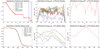
Fig. 3 Density distribution across the entire domain for PIROCK with different tolerances, the explicit approach, and reference solutions (top left). The top-middle panel depicts the distribution of the logarithm of the absolute difference, log10(|ρ − ρref|), between the different scenarios and the reference solution. The top-right panel shows the distribution of the logarithm of the absolute difference between analytical and reference solution log10(|ρ − ρref|). The bottom panels mirror the top ones but focus specifically on the shock region between x=0.82 and 0.88 (indicated by the two vertical blue lines in the top-left panel). The red dashed line represents the reference solution, and the black dashed line corresponds to the explicit. The remaining colors represent different PIROCK cases with varying tolerances.
The “operator splitting” approach, denoted as splitting, follows the methodology as outlined by Wargnier et al. (2023). In this approach, FA and artificial hyperdiffusive terms are integrated using an RK3-2N method, the Spitzer term is integrated using a wave method, as described by Rempel (2017), and the source terms are integrated implicitly through a fifthorder implicit Runge Kutta method also known as Radau IIA method (see Hairer & Wanner 1999, 1996). The coupling of these terms is handled using a first-order Lie splitting approach.
The following comparative analysis demonstrates the suitability of the PIROCK method for both multi-fluid and single-fluid MHD models and its potential benefits in terms of computational cost savings.
We initially focus on a 1D single-fluid Sod-Shock tube problem for this comparison. We compare the explicit approach with PIROCK for different tolerances, evaluating the computational cost versus accuracy between the two methods. We aim to comprehend how PIROCK determines the number of stages s for this type of problem and how it stabilizes the scheme while significantly reducing computational cost by executing fewer steps than the explicit approach.
In the following investigation, we explore a 2.5 D reconnection scenario utilizing an MFMS model. Our analysis begins by examining various species involved, including {H, H+, He, He+ 𝔢}. Through comparative analysis, we assess the performance of the PIROCK method with different tolerances and compare it with the splitting and explicit.
6.1 Sod shock
In this section, we analyze a Sod Shock problem following Sod (1978). We compare PIROCK cases (with tolerances from tol = 10−2 to tol = 10−5 and an extra case at tol = 10−8) with an explicit calculation to evaluate their performance in a purely hyperbolic problem. We consider only the advective part of the system of Eqs. (1) for a 1D hydrodynamic single-fluid with artificial hyperdiffusion. Therefore, the system involves a single set of continuity, momentum, and energy equations, represented by the conservative variables vector Y = (ρ,ρux, e).
6.1.1 Initial conditions
The initial left and right state of the vector Y in the Sod-Shock problem is described by
![$\[\mathbf{Y}_L=\left(1,0, \frac{1}{(\gamma-1)}\right)^T \text { and } \mathbf{Y}_R=\left(0.125,0, \frac{0.1}{(\gamma-1)}\right)^T,\]$](/articles/aa/full_html/2025/03/aa52351-24/aa52351-24-eq37.png) (18)
(18)
where γ = 1.4. We consider a smooth initial solution where the two states YL and YR are connected by the following hyperbolic tangent:
![$\[\mathbf{f}(x)=\left(\frac{\mathbf{Y}_L+\mathbf{Y}_R}{2}\right)+\left(\frac{\mathbf{Y}_L-\mathbf{Y}_R}{2}\right) \tanh \left(\frac{x-0.5}{\lambda}\right),\]$](/articles/aa/full_html/2025/03/aa52351-24/aa52351-24-eq38.png) (19)
(19)
where x ∈ [0, 1] and λ = 10−2. We ran simulations for all PIROCK and explicit cases until t = tf = 0.2. We consider a uniform mesh of 256 grid points.
A reference solution was constructed utilizing the explicit case with an extremely small fixed timestep of Δt = 10−9 for method comparison. Additionally, we compared our results with the classical analytical solution of the Sod-Shock problem that considers discontinuous initial conditions instead of a smooth hyperbolic tangent.
To be consistent with what is generally used in Bifrost (e.g., Martínez-Sykora et al. 2020; Nóbrega-Siverio et al. 2016, 2017), we have chosen the hyperdiffusive terms coefficients ν1 = ν2 = 0.2 and ν3 = 0.3 in Eq. (6) for all cases.
6.1.2 Comparative analysis of all methods
Figure 3 illustrates the density distribution for all cases. The topleft panel displays the distribution of numerical solutions for the entire domain, while the top-middle panel shows the difference from the reference solution. The top-right panel shows the difference between the reference and analytical solution of the density. The bottom panels zoom on the region between x = 0.82 and 0.88, indicated by the two vertical blue lines around the shock wave in the top-left panel. This emphasis highlights differences in the solution in this region, where the error and L2 norm are maximized.
All cases (including various tolerances of PIROCK and the explicit case) successfully capture the characteristic waves and jump conditions of the Sod-Shock test case, as compared with the analytical solution (top-left panel of Fig. 3). The tolerance decreases, and the difference between the numerical solution for the PIROCK cases and the reference solution diminishes (top-middle panel). This trend is further emphasized when focusing on the shock region (bottom row of Fig. 3). Higher tolerances (10−2 and 10−3) yield a slightly more diffusive solution compared to lower tolerances.
Table 1 compares various parameters between the explicit and PIROCK cases for different tolerances. Specifically, we assess the number of steps to reach t = tf, the average timestep ![$\[\overline{\Delta t}\]$](/articles/aa/full_html/2025/03/aa52351-24/aa52351-24-eq40.png) chosen by each method, the number of evaluations for the hyperdiffusion term FD and the advection term FA, the maximum number of stages s selected by PIROCK during the simulation, the L2 norm between the numerical and reference solutions for the density variable ρ, the average CPU time per step for each case and the total computational time.
chosen by each method, the number of evaluations for the hyperdiffusion term FD and the advection term FA, the maximum number of stages s selected by PIROCK during the simulation, the L2 norm between the numerical and reference solutions for the density variable ρ, the average CPU time per step for each case and the total computational time.
In our study, we observed that the explicit case necessitates 2203 steps to achieve an average timestep of Δt = 8.76 × 10⁻⁵, yielding a L2 norm of the density of 2 × 10⁻⁶, with a total computational time of 13.2 s. Transitioning to the PIROCK case with the highest tolerance (10−2 or 10−3), we managed to reduce the total computational cost to 3.8 s, requiring only 160 steps. However, this optimization comes at the expense of a higher L2 norm of the density, measured at 7.6 × 10⁻⁵. As the tolerance decreases further (10−4 or 10−5), we noted an increase in computational cost (from 3.9 to 5.1 s) alongside a decrease in the L2 norm (ranging from 3.4 × 10⁻⁵ to 10−5). This trend aligns with the underlying principles of the PIROCK approach, which is expected to refine the solution as the tolerance diminishes. Additionally, our findings suggest the possibility of achieving a superior approximation of the solution compared to the explicit 3 rd order method by further reducing the tolerance to 10−8.
As depicted in Table 1, an increase in tolerance prompts a corresponding increase in the maximum number of stages (smax). Specifically, for tolerances ranging from 10−4 to 10−2, the number of stages rises to 10 and 12, respectively, compared to mere counts of 1 and 4 for tolerances of 10−8 and 10−5. This observed behavior is attributed to PIROCK’s dynamic adjustment of the stage number s while maintaining an approximation error (err) close to the prescribed user tolerance (tol). When the tolerance is increased, the PIROCK algorithm allows for a larger timestep and optimally adjusts the number of stages while remaining in the stability domain of the diffusive terms. We note that the explicit method is restricted not only from the CFL condition of the advective term but also from the hyperdiffusive terms. However, PIROCK solves the hyperdiffusive terms with the ROCK2 method.
In summary, PIROCK allows for fine-tuning solution quality and computational costs through user-defined tolerance. The method demonstrates superior efficiency, requiring substantially fewer steps than the explicit approach. The explicit approach takes 13.3 s compared to 3.8 seconds for the highest tolerance tol = 10−2. The achieved solution quality remains highly satisfactory relative to the number of steps taken, establishing PIROCK as a more efficient alternative to the explicit approach even for a classical Sod-Shock test.
Comparative analysis of the explicit and PIROCK methods with varying tolerances.
Initial number densities in the 2.5 D reconnection problem.
6.2 Problem of 2.5 dimensional reconnection
As previously outlined, our initial endeavor entails addressing a significant magnetic reconnection challenge involving four distinct species: {H, H+, He, He+}, with initial number densities presented in Table 2. Extending upon our previous study investigating magnetic reconnection with four species (see Wargnier et al. 2023), our objective is to showcase the applicability of the PIROCK method on the MFMS model in addressing complex solar physics phenomena involving multiple species, while maintaining computational efficiency. We compare with conventional methods such as explicit and splitting.
Comparative analysis of all methods, including the splitting, explicit, and PIROCK methods with varying tolerances.
Comparison of L2 norm of the error of the species density relative to splitting, explicit and PIROCK methods (tolerances tol = 10−2 and 10−5).
6.2.1 Initial conditions
We consider a reconnection problem with identical thermodynamic conditions but different box sizes and mixtures. The initial thermodynamic conditions for the 2.5D reconnection problem are based on those in Wargnier et al. (2023) (Section 4.1), with T0 = 16 000 K, n0 = 4.8 × 109 cm−3, and plasma beta βp = 0.1.
To compare the methods efficiently without performing an extensive analysis, we use a smaller computational domain. The smaller domain is necessary because the explicit and splitting methods are computationally very expensive, as shown below. The domain lengths in the y and z directions, denoted as Ly and Lz, are 1.5 Mm and 3 Mm, respectively, with Δy = 100 km and Δz = 75 km, resulting in a grid of 150 × 400 points and a magnetic field strength B0 = 2 G.
It is important to note that, unlike Wargnier et al. (2023), we have considered periodic boundary conditions along the z direction and open boundary conditions in the y direction, and the Hall term is taken into account. We compared the PIROCK method (tol = 10−2 and 10−5) with the splitting and explicit methods up to t = 200 s.
6.2.2 Comparative analysis of numerical methods
A reference solution was constructed using a fixed timestep of Δt = 10−8 s. The method used for this reference solution was a third-order Runge–Kutta scheme for the differential and advective terms (FD and FA), and an implicit scheme, similar to PIROCK, for the reactive term (FR).
In Table 3, we compared the methods splitting, explicit, and PIROCK (with tolerances 10−2 and 10−5) across various aspects such as the number of steps, average timestep value, number of function evaluations, maximum number of stages (smax), average computational cost per step, and total computational cost of the simulation. The results clearly demonstrate the efficiency of the PIROCK method in terms of computational cost. Specifically, the number of steps required for PIROCK (3000 for tol = 10−2 and 12 000 for tol = 10−5) is significantly lower compared to explicit (1 000 000 steps) and splitting (800 000 steps). The average timestep (1.5 × 10⁻⁴ and 4.8 × 10⁻⁵) for PIROCK is at least three orders of magnitude larger than for explicit (4.59 × 10⁻⁷) and splitting (5.7 × 10⁻⁷). Even though the computational cost per step is higher, the total computational cost for PIROCK is dramatically lower than for the splitting and the explicit by almost two orders of magnitude.
In Table 4, we present the L2 norm for all densities of the model compared to the reference solution. It is observed that for all species, the L2 norm is similar or slightly better for PIROCK. This indicates that for a much lower computational cost, we achieve nearly the same precision (or better) for the density. However, the improvement in precision between the tolerances 10−2 and 10−5 is not significant.
Figures 4 and 5 illustrate the final time distribution of the velocity uz,H and the density ρH, along with a 2 D comparison of the difference between the reference and the solution obtained for each method. Focusing on Fig. 4, we observe that the error is primarily localized in the current sheet, the outflow regions of the reconnection, and strong discontinuities (near plasmoids) and shocks. However, PIROCK appears to capture the solution better in these shock regions, as shown by the 1D distribution (bottom panel). It is also evident that splitting is quite imprecise compared to the other methods. This imprecision arises because we use a first-order Lie splitting, which introduces a first-order temporal error, making the method much less accurate than the explicit and PIROCK methods, which are of orders 3 and 2, respectively. Similar results are obtained for all other variables.
PIROCK proves to be highly efficient regarding both computational cost and accuracy for all variables. The number of steps is significantly reduced, allowing for a much larger timestep and a drastically lower computational cost than traditional splitting and explicit methods.
6.2.3 Fluxes calculation and chemical fractionation
In this section, we demonstrate the capabilities of PIROCK in efficiently solving multi-fluid reconnection problems. As an example, we quantify the chemical fractionation between hydrogen and helium during magnetic reconnection. We conduct a study similar to Wargnier et al. (2023) but with significant differences. In our case, the flux calculations in the outflow (z) direction are performed over a much larger domain, which promotes increased plasmoid formation. Additionally, periodic boundaries are used instead of open boundaries throughout the entire setup.
Additionally, the grid size and resolution of the current sheet are different; we note here that the spatial resolution is 150x400 grid points, with Δy = 100 km and Δz = 75 km, whereas in Wargnier et al. (2023) it was 800x800 with Δy = Δz = 5.33 km. Moreover, although the domain is periodic in the z-direction, we have verified that the boundary conditions do not influence these flux calculations.
To characterize the chemical fractionation in the outflows, similar to Wargnier et al. (2023), the fluxes of helium and hydrogen species have been calculated and compared at the exhaust of the reconnection event until t = 180 s. These calculations are conducted at fixed heights of zi = 1.9 Mm and 1.7 Mm. For any species α, the corresponding flux in number density is calculated as
![$\[\phi(\alpha)=\Delta t \Delta x \int_{l_y}\left[u_{z, \alpha} n_\alpha\right]\left(y, z=z_i\right) d y,\]$](/articles/aa/full_html/2025/03/aa52351-24/aa52351-24-eq45.png) (20)
(20)
where Δx is the grid size in the x direction (set to unity), and ly is the length in the y direction limited to the outflow region. The outflow regions are defined as the FWHM of the maximum outflow velocity at z = zi. This length is obtained by locating the maximum outflow velocity at z = zi, and the termination of the exhaust is approximated at 90% of this maximum in the y direction to estimate ly.
In Fig. 6, which shows the time evolution of the flux ratio ϕ(He + He+)/(ϕ(He + He+) + ϕ(H + H+)) at different heights, z = 1.7 Mm and z = 1.9 Mm, we observe significant changes in the flux distribution as the reconnection evolves. Focusing on the black curve at z = 1.7 Mm, as turbulence develops with the formation of plasmoids and shocks, the helium flux increases significantly relative to the total flux. This indicates that during the passage of shocks, a higher fraction of helium is produced than hydrogen, with the flux ratio reaching up to 42%, as observed around t ≈ 140 s during a plasmoid event.
As the shock propagates and reaches z = 1.9 Mm (red curve), a similar increase in helium flux can be seen, corresponding to earlier events at z = 1.7 Mm. For example, the rise in flux at t ≈ 140 s in the black curve corresponds to a peak at t = 150 s in the red curve. This suggests the presence of multiple shocks and plasmoids propagating and causing peaks in the flux ratio. The helium fraction increases significantly during turbulent reconnection. The mechanism explaining this increase is similar to what is described in Wargnier et al. (2023). Briefly, during the laminar phase, the ionization fraction of hydrogen is higher, and hydrogen is slowly expelled, with relatively small outflows. However, in the turbulent phase, characterized by stronger flows and the formation of plasmoids, the number of helium elements increases, and helium is ionized due to the temperature rise, resulting in an enrichment of helium in the outflows. The difference, as explained earlier, lies in the resolution, the number of grid points, the domain size, and the evolution of the magnetic field topology due to the periodic boundary conditions, which are distinct between the two cases.
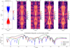 |
Fig. 4 Top, far left: distribution of the reference solution of the velocity uz,H in a restricted domain along the y direction (y ∈ [0.2, 0.8] Mm) in km s−1. Top, center and right: two-dimensional figures representing represent the logarithm of the difference between the reference and the numerical solution |
![$\[\log _{10}\left(u_{z, H}^{r e f}-u_{z, H}\right)\]$](/articles/aa/full_html/2025/03/aa52351-24/aa52351-24-eq43.png)
![$\[\log _{10}\left(u_{z, H}^{r e f}- u_{z, H}\right)\]$](/articles/aa/full_html/2025/03/aa52351-24/aa52351-24-eq44.png)
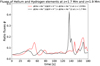 |
Fig. 6 Time evolution of the flux ratio of helium species relative to the total flux of all species, ϕ(He + He+)/(ϕ(He + He+) + ϕ(H + H+)), at two different locations, z = 1.7 Mm (black line) and z = 1.9 Mm (red line). |
7 Conclusion
This study concentrated on devising a novel and efficient temporal integration method tailored to the multi-fluid MHD model. The latter has been introduced and reformulated as a set of ordinary differential equations, elucidating the diffusive, convective, and stiff source terms within the model. However, we point out that the outlined numerical strategy holds applicability to any single or multi-fluid MHD system provided that we can reformulate the system of equations as a stiff reaction-diffusive-convective set of equations. Notably, the numerical strategy remains agnostic to the specifics of spatial discretization.
We presented an overview of Runge–Kutta methods commonly used for integrating diffusive, stiff reactive, and advective terms, aiming to identify the most suitable numerical time integration method. In solar and stellar physics, while various methods excel in integrating stiff reactive or advective terms, diffusive terms pose a primary challenge. In this work, we introduce, for the first time in the context of solar and stellar physics, the well-known ROCK2 method. This approach is particularly attractive due to its explicit, second-order, and competitive nature with implicit schemes. Another challenge is integrating diffusion-advection and reactive terms simultaneously. Traditional approaches such as time operator splitting have been considered, albeit with known splitting errors and stability issues for multiple stiff terms. We focus on the PIROCK method, developed by Abdulle & Vilmart (2013a), an implicit-explicit partitioned Runge–Kutta method, for integrating diffusive, stiff reactive, and advective terms altogether. PIROCK combines ROCK2 for diffusion, SDIRK for stiff reactive terms, and a third-order Heun method for advective terms, incorporating an adaptive timestep strategy and error calculations using methods introduced by Hairer et al. (1993). It is important to note that the artificial hyperdiffusive terms in the model are integrated using the ROCK2 method simultaneously with all other physical diffusion terms.
We conducted a comparative analysis of the PIROCK method against two other approaches: a purely explicit method using a 3rd-order Runge–Kutta scheme with an explicit integration of reactive and diffusive terms and a splitting approach employing Lie Splitting identically to Wargnier et al. (2023). Focusing initially on a single-fluid MHD Sod-Shock tube problem, we assessed the explicit and PIROCK methods for varying tolerances. Results demonstrate that user-defined tolerances effectively regulate solution quality and computational cost, as expected. By choosing to integrate hyperdiffusive terms within the ROCK2 part of PIROCK, it becomes possible to control the quality of the numerical solution, especially in shocks and discontinuities, using the properties of embedded methods, which is not achievable with standard explicit methods due to the timestep being always limited by the CFL constraint of hyperdiffusive terms. In this context, it is feasible to reduce the computational cost from 13.3 s (2203 steps) to just 3.8 s (160 steps) (for tol = 10−2) with a loss of accuracy from 2 × 10⁻⁶ to 7.6 × 10⁻⁵ as detailed in Table 1. However, we emphasize that the solution quality remains highly satisfactory, and this loss of precision is simply associated with increased diffusion and regularization around discontinuities and shocks. In this respect, PIROCK demonstrates greater flexibility (regarding computational cost versus accuracy) compared to the traditional explicit approach that involves hyperdiffusive terms.
Next, we focused on a 2D multi-fluid reconnection problem involving multiple species {H, H+, He, He+} with the complete model including all terms. Results show that PIROCK outperforms splitting and explicit for all variables compared to our constructed reference solution. Regarding computational cost only, PIROCK outperforms splitting and is more than one, almost two, orders of magnitude faster for the highest tolerances. PIROCK has a slightly higher per-step computational cost due to the high number of source term evaluations FR and the chosen number of stages s for the integration of diffusive terms with ROCK2. Nevertheless, at a tolerance of 10−2, PIROCK requires only 3306 steps to reach the final time t = tf = 50s, whereas splitting requires 821 974, hence a number of timesteps reduced by a factor 250. Concerning accuracy, it is clear that PIROCK outperforms the standard splitting approach, and the latter shows an excess of diffusion, especially close to shocks and discontinuities. The excessive diffusion in the splitting approach is attributed to first-order temporal errors due to the Lie splitting error, while PIROCK is a second-order scheme.
Finally, thanks to this new numerical method, we are now able to tackle complex multi-fluid problems that were previously unsolvable in reasonable computational time. We have demonstrated the ability of our numerical model to address chemical fractionation between hydrogen and helium species in the context of magnetic reconnection. Our results highlight the decoupling of species when the reconnection regime becomes turbulent similarly, as in Wargnier et al. (2023). These cases show the potential of the numerical model for future multi-fluid applications such as the first-ionization-potential (FIP) effect, which required more fluids (high and low FIP elements) and is now feasible thanks to PIROCK. The latter will be investigated in a follow-up paper.
In summary, the PIROCK method exhibits remarkable superiority over conventional approaches such as standard splitting methods and standard explicit methods in terms of accuracy, stability, and computational efficiency, regardless of tolerance levels. This superiority is evident across various scenarios, including typical two-dimensional solar physics situations and hyperbolic Sod shock problems, covering both the multi-fluid system of equations (1) and the single-fluid approach. These findings underscore the method’s exceptional performance compared to established classical time integration methods. The advances introduced by PIROCK will be highly beneficial to NASA’s Interface Region Imaging Spectrograph satellite mission which observes how the low solar atmosphere is energized, but heavily depends on numerical simulations to interpret the observations. PIROCK will lead to much improved computational efficiency for numerical simulations that benefit IRIS and other NASA missions, such as the future MUlti-Slit Solar Explorer (MUSE, De Pontieu et al. 2020), which is focused on a better understanding of the solar corona.
Acknowledgements
The authors would like to thank Ernst Hairer for helpful discussions. This project received partial financial support from NASA grants 80NSSC21K0737, 80NSSC21K1684, and contracts NNG09FA40C (IRIS) and 80GSFC21C0011 (MUSE). The simulations have been run in the Pleiades cluster through the computing projects s1061, s2601, and s2967 from the High-End Computing (HEC) division of NASA. The second author was partially supported by the Swiss National Science Foundation, projects No. 200020_214819, and No. 200020_192129.
Appendix A ROCK2 algorithm for diffusive terms
For a given number of stage s > 1 and an initial condition Y0, the ROCK2 time integration method applies to the problem ![$\[\frac{d \mathbf{Y}(t)}{d t}= \mathbf{F}_{\mathrm{D}}(\mathbf{Y}(t))\]$](/articles/aa/full_html/2025/03/aa52351-24/aa52351-24-eq46.png) with initial condition Y0, reads
with initial condition Y0, reads
![$\[\begin{aligned}\mathbf{Y}_1 & =\mathbf{Y}_0+\alpha \mu_1 \Delta t \mathbf{F}_{\mathrm{D}}\left(\mathbf{Y}_0\right) \\\mathbf{Y}_j & =\alpha \mu_j \Delta t \mathbf{F}_{\mathrm{D}}\left(\mathbf{Y}_{j-1}\right)-\nu_j \mathbf{Y}_{j-1}-\kappa_j \mathbf{Y}_{j-2}, \\\mathbf{Y}_{s-1} & =\mathbf{Y}_{s-2}+\sigma_s \Delta t \mathbf{F}_{\mathrm{D}}\left(\mathbf{Y}_{s-2}\right) \\\mathbf{Y}_s & =\mathbf{Y}_{s-1}+\sigma_s \Delta t \mathbf{F}_{\mathrm{D}}\left(\mathbf{Y}_{s-1}\right) \\\mathbf{Y}_n & =\mathbf{Y}_s-\sigma_s \Delta t\left(1-\frac{\tau_s}{\sigma_s^2}\right) \Delta \mathbf{F}_{\mathrm{D}}^s \\\Delta \mathbf{F}_{\mathrm{D}}^s & =\left[\mathbf{F}_{\mathrm{D}}\left(\mathbf{Y}_{s-1}\right)-\mathbf{F}_{\mathrm{D}}\left(\mathbf{Y}_{s-2}\right)\right],\end{aligned}\]$](/articles/aa/full_html/2025/03/aa52351-24/aa52351-24-eq47.png) (ID)
(ID)
where j = 2, . . ., s − 2, μj, vj and κj are obtained from the Chebyshev recurrence relation of the orthogonal Chebyshev polynomials (as described in Eqs. 24-25 from Abdulle & Medovikov (2001) and defined as {Pj}j≥0 in Abdulle & Vilmart (2013a)), and Yn is the vector conservative variables after integration. We note that the Chebyshev polynomials {Pj}j≥0 are the stability functions of each internal stage of the ROCK2 method (Eq. (ID)). The original ROCK2 methods uses α = 1 while we use a parameter α > 1 in PIROCK. The values of the coefficients σs and τs depend on the total number of stage s and are chosen such that they satisfy second order accuracy of the method for any s.
Appendix B 2-stage second-order Singly Diagonally Implicit Runge–Kutta (SDIRK) method for source terms
The 2-stage second-order and L-stable Singly Diagonally Implicit Runge–Kutta (SDIRK) method applies to the problem ![$\[\frac{d \mathbf{Y}(t)}{d t}=\mathbf{F}_{\mathrm{R}}(\mathbf{Y}(t))\]$](/articles/aa/full_html/2025/03/aa52351-24/aa52351-24-eq48.png) with initial condition Y0, reads
with initial condition Y0, reads
![$\[\begin{aligned}& \mathbf{Y}_1=\mathbf{Y}_0+\gamma \Delta t \mathbf{F}_{\mathrm{R}}\left(\mathbf{Y}_1\right) \\& \mathbf{Y}_2=\mathbf{Y}_0+(1-2 \gamma) \Delta t \mathbf{F}_{\mathrm{R}}\left(\mathbf{Y}_1\right)+\gamma \Delta t \mathbf{F}_{\mathrm{R}}\left(\mathbf{Y}_2\right) \\& \mathbf{Y}_n=\mathbf{Y}_0+\frac{\Delta t}{2} \mathbf{F}_{\mathrm{R}}\left(\mathbf{Y}_1\right)+\frac{\Delta t}{2} \mathbf{F}_{\mathrm{R}}\left(\mathbf{Y}_2\right),\end{aligned}\]$](/articles/aa/full_html/2025/03/aa52351-24/aa52351-24-eq49.png) (IR)
(IR)
where ![$\[\gamma=1-\sqrt{2} / 2\]$](/articles/aa/full_html/2025/03/aa52351-24/aa52351-24-eq50.png) and Yn is the vector of conservative variables after integration.
and Yn is the vector of conservative variables after integration.
Appendix C PIROCK algorithm
C.1 Scenario with Dominant Diffusive Processes (s > 1)
For thoroughness, we present the formulation of the PIROCK method, when s > 1 with initial condition Y0, for the integration of the complete system in Eq. (1), as detailed in Abdulle & Vilmart (2013a),
Diffusion stabilization procedure:
![$\[\begin{aligned}& \mathbf{Y}_1=\mathbf{Y}_0+\alpha \mu_1 ~\Delta t \mathbf{F}_{\mathrm{D}}\left(\mathbf{Y}_0\right) \\& \mathbf{Y}_j=\alpha \mu_j \Delta t \mathbf{F}_{\mathrm{D}}\left(\mathbf{Y}_{j-1}\right)-v_j \mathbf{Y}_{j-1}-\kappa_j \mathbf{Y}_{j-2}, \quad j=2, \ldots, s-1.\end{aligned}\]$](/articles/aa/full_html/2025/03/aa52351-24/aa52351-24-eq51.png)
Finishing procedure for diffusion (additional two steps):
![$\[\begin{aligned}& \widetilde{\mathbf{Y}}_{s-1}=\mathbf{Y}_{s-2}+\sigma_s \Delta t \mathbf{F}_{\mathrm{D}}\left(\mathbf{Y}_{s-2}\right), \\& \widetilde{\mathbf{Y}}_s=\widetilde{\mathbf{Y}}_{s-1}+\sigma_s \Delta t \mathbf{F}_{\mathrm{D}}\left(\widetilde{\mathbf{Y}}_{s-1}\right).\end{aligned}\]$](/articles/aa/full_html/2025/03/aa52351-24/aa52351-24-eq52.png)
Integration of advective-reaction terms and coupling with diffusion:
![$\[\begin{aligned}\mathbf{Y}_{s+1} & =\mathbf{Y}_{s-1}+\gamma \Delta t \mathbf{F}_{\mathrm{R}}\left(\mathbf{Y}_{s+1}\right) \\\mathbf{Y}_{s+2} & =\mathbf{Y}_{s-1}+\Delta t(1-2 \gamma) \mathbf{F}_{\mathrm{R}}\left(\mathbf{Y}_{s+1}\right)+\Delta t \gamma \mathbf{F}_{\mathrm{R}}\left(\mathbf{Y}_{s+2}\right)+\Delta t \mathbf{F}_{\mathrm{A}}\left(\mathbf{Y}_{s+1}\right), \\\mathbf{Y}_{s+3} & =\mathbf{Y}_{s-1}+\Delta t(1-2 \gamma) \mathbf{F}_{\mathrm{A}}\left(\mathbf{Y}_{s+1}\right)+\Delta t(1-\gamma) \mathbf{F}_{\mathrm{R}}\left(\mathbf{Y}_{s+1}\right), \\\mathbf{Y}_{s+4} & =\mathbf{Y}_{s-1}+\frac{\Delta t}{3} \mathbf{F}_{\mathrm{A}}\left(\mathbf{Y}_{s+1}\right), \\\mathbf{Y}_{s+5}= & \mathbf{Y}_{s-1}+\frac{2 \Delta t}{3} \mathbf{J}_{\mathrm{R}}^{-1} \mathbf{F}_{\mathrm{A}}\left(\mathbf{Y}_{s+4}\right)+\Delta t\left(\frac{2}{3}-\gamma\right) \mathbf{F}_{\mathrm{R}}\left(\mathbf{Y}_{s+1}\right) \\& +\frac{\Delta t 2 \gamma}{3} \mathbf{F}_{\mathrm{R}}\left(\mathbf{Y}_{s+2}\right).\end{aligned}\]$](/articles/aa/full_html/2025/03/aa52351-24/aa52351-24-eq53.png)
Final integration from Y0 to Yn:
![$\[\begin{aligned}\mathbf{Y}_n= & \widetilde{\mathbf{Y}}_s-\sigma_s \Delta t\left(1-\frac{\tau_s}{\sigma_s^2}\right)\left[\mathbf{F}_{\mathrm{D}}\left(\widetilde{\mathbf{Y}}_{s-1}\right)-\mathbf{F}_{\mathrm{D}}\left(\mathbf{Y}_{s-2}\right)\right] \\& +\frac{\Delta t}{4} \mathbf{F}_{\mathrm{A}}\left(\mathbf{Y}_{s+1}\right)+\frac{3 \Delta t}{4} \mathbf{F}_{\mathrm{A}}\left(\mathbf{Y}_{s+5}\right) \\& +\frac{\Delta t}{2} \mathbf{F}_{\mathrm{R}}\left(\mathbf{Y}_{s+1}\right)+\frac{\Delta t}{2} \mathbf{F}_{\mathrm{R}}\left(\mathbf{Y}_{s+2}\right) \\& +\frac{\Delta t \mathbf{J}_{\mathrm{R}}^{-1}}{2-4 \gamma}\left[\mathbf{F}_{\mathrm{D}}\left(\mathbf{Y}_{s+3}\right)-\mathbf{F}_{\mathrm{D}}\left(\mathbf{Y}_{s+1}\right)\right],\end{aligned}\]$](/articles/aa/full_html/2025/03/aa52351-24/aa52351-24-eq54.png) (P)
(P)
where ![$\[\mathbf{J}_{\mathrm{R}}=\mathbb{I}-\gamma \Delta t \frac{\partial \mathbf{F}_{\mathrm{R}}}{\partial \mathbf{Y}}\left(\mathbf{Y}_{s-1}\right), \gamma, \tau_{s}, \sigma_{s}, \nu_{j}, \kappa_{j}\]$](/articles/aa/full_html/2025/03/aa52351-24/aa52351-24-eq55.png) and μj are coefficients that have been described in Sections A and B,
and μj are coefficients that have been described in Sections A and B, ![$\[\alpha=1 /\left(2 P_{s-1}^{\prime}(0)\right)\]$](/articles/aa/full_html/2025/03/aa52351-24/aa52351-24-eq56.png) (chosen such that the internal stage Ys−1 integrates the diffusion part alone for half stepsize
(chosen such that the internal stage Ys−1 integrates the diffusion part alone for half stepsize ![$\[\alpha P_{s-1}^{\prime}(0) \Delta t=\Delta t / 2)\]$](/articles/aa/full_html/2025/03/aa52351-24/aa52351-24-eq57.png) and Yn is the vector of conservative variable after integration. We note that the PIROCK algorithm P is identical to the one presented in Abdulle & Vilmart (2013a) where we choose the particular case where α > 1 and stage parameter s given in Eq. (17) (due to the stability domain size 0.43s2 along the negative real axis for the diffusion terms). We emphasize the negligible computational expense incurred in computing
and Yn is the vector of conservative variable after integration. We note that the PIROCK algorithm P is identical to the one presented in Abdulle & Vilmart (2013a) where we choose the particular case where α > 1 and stage parameter s given in Eq. (17) (due to the stability domain size 0.43s2 along the negative real axis for the diffusion terms). We emphasize the negligible computational expense incurred in computing ![$\[\mathbf{J}_{\mathrm{R}}^{-1}\]$](/articles/aa/full_html/2025/03/aa52351-24/aa52351-24-eq58.png) , where
, where ![$\[\mathbf{J}_{\mathrm{R}}^{-1}\]$](/articles/aa/full_html/2025/03/aa52351-24/aa52351-24-eq59.png) represents the inverse of the Jacobian matrix tied to the source terms FR. This efficiency stems from the fact that the LU factorization of the Jacobian JR is readily obtainable during the computation of the implicit stages of FR.
represents the inverse of the Jacobian matrix tied to the source terms FR. This efficiency stems from the fact that the LU factorization of the Jacobian JR is readily obtainable during the computation of the implicit stages of FR.
C.2 Scenario where s = 1
In contrast to the preceding subsection, we now examine the PIROCK case with s = 1. This corresponds to a scenario where the dominant advective process within the same system (S) is considered. For an initial condition Y0, the algorithm in this context is as follows:
![$\[\begin{aligned}\mathbf{Y}_1= & \mathbf{Y}_0+\gamma \Delta t \mathbf{F}_{\mathrm{R}}\left(\mathbf{Y}_1\right), \\\mathbf{Y}_2= & \mathbf{Y}_0+\Delta t(1-2 \gamma) \mathbf{F}_{\mathrm{R}}\left(\mathbf{Y}_1\right)+\Delta t \gamma \mathbf{F}_{\mathrm{R}}\left(\mathbf{Y}_2\right) \\& +\Delta t \mathbf{F}_{\mathrm{A}}\left(\mathbf{Y}_1\right)+\Delta t \mathbf{F}_{\mathrm{D}}\left(\mathbf{Y}_1\right), \\\mathbf{Y}_3= & \mathbf{Y}_0+\frac{\Delta t}{3} \mathbf{F}_{\mathrm{A}}\left(\mathbf{Y}_1\right)+\frac{\Delta t}{3} \mathbf{F}_{\mathrm{D}}\left(\mathbf{Y}_1\right), \\\mathbf{Y}_n= & \mathbf{Y}_0+\frac{2 \Delta t}{3} \mathbf{J}_{\mathrm{R}}^{-1}\left(\mathbf{F}_{\mathrm{A}}\left(\mathbf{Y}_3\right)+\mathbf{F}_{\mathrm{D}}\left(\mathbf{Y}_3\right)\right) \\& +\Delta t\left(\frac{2}{3}-\gamma\right) \mathbf{F}_{\mathrm{R}}\left(\mathbf{Y}_1\right)+\frac{\Delta t 2 \gamma}{3} \mathbf{F}_{\mathrm{R}}\left(\mathbf{Y}_2\right),\end{aligned}\]$](/articles/aa/full_html/2025/03/aa52351-24/aa52351-24-eq60.png) (P2)
(P2)
where ![$\[\gamma=1-\sqrt{2} / 2\]$](/articles/aa/full_html/2025/03/aa52351-24/aa52351-24-eq61.png) and Yn is the vector of conservative variables after integration.
and Yn is the vector of conservative variables after integration.
References
- Abdulle, A. 2002, SIAM J. Sci. Comput., 23, 2041 [CrossRef] [Google Scholar]
- Abdulle, A. 2015, Explicit Stabilized Runge–Kutta Methods (Springer Berlin Heidelberg: Encyclopedia of Applied and Computational Mathematics), 460 [Google Scholar]
- Abdulle, A., & Li, T. 2008, Commun. Math. Sci., 6, 845 [CrossRef] [Google Scholar]
- Abdulle, A., & Medovikov, A. A. 2001, Numer. Math., 90, 1 [CrossRef] [Google Scholar]
- Abdulle, A., & Vilmart, G. 2013a, J. Comput. Phys., 242, 869 [Google Scholar]
- Abdulle, A., & Vilmart, G. 2013b, Yareta [Fortran source code], https://doi.org/10/grp98q [Google Scholar]
- Alexander, R. 1977, SIAM J. Numer. Anal., 14, 1006 [NASA ADS] [Google Scholar]
- Alvarez Laguna, A., Lani, A., Deconinck, H., Mansour, N. N., & Poedts, S. 2016, J. Comput. Phys., 318, 252 [NASA ADS] [CrossRef] [Google Scholar]
- Ballester, J. L., Alexeev, I., Collados, M., et al. 2018, Space Sci. Rev., 214, 58 [Google Scholar]
- Brandenburg, A., Johansen, A., Bourdin, P. A., et al. 2021, J. Open Source Softw., 6, 2807 [CrossRef] [Google Scholar]
- Butcher, J. 1996, Appl. Numer. Math., 20, 247 [Google Scholar]
- Caplan, R. M., Johnston, C. D., Daldoff, L. K. S., & Linker, J. A. 2024, J. Phys. Conf. Ser., 2742, 012020 [Google Scholar]
- Carpenter, M. H., & Kennedy, C. A. 1994, NASA Technical Memorandum; National Aeronautics and Space Administration, Langley Research Center [National Technical Information Service, distributor] [Google Scholar]
- De Pontieu, B., Martínez-Sykora, J., Testa, P., et al. 2020, ApJ, 888, 3 [NASA ADS] [CrossRef] [Google Scholar]
- Descombes, S., Duarte, M., Dumont, T., Louvet, V., & Massot, M. 2011, Confluentes Math., 03, 413 [Google Scholar]
- Descombes, S., Duarte, M., Dumont, T., et al. 2014, SIAM J. Numer. Anal., 52, 1311 [Google Scholar]
- Duarte, M. 2011, PhD thesis, Ecole Centrale Paris, France, https://tel.archives-ouvertes.fr/tel-00667857 [Google Scholar]
- Duarte, M., Massot, M., Descombes, S., et al. 2012, SIAM J. Sci. Comput., 34, A76 [NASA ADS] [Google Scholar]
- Genevi, V. A., Alexiades, V., Amiezy, G., & Gremaudz, P.-A. 1996, Commun. Num. Meth. Eng., 12, 12 [Google Scholar]
- González-Morales, P. A., Khomenko, E., Downes, T. P., & de Vicente, A. 2018, A&A, 615, A67 [Google Scholar]
- Gudiksen, B. V., Carlsson, M., Hansteen, V. H., et al. 2011, A&A, 531, A154 [NASA ADS] [CrossRef] [EDP Sciences] [Google Scholar]
- Guillou, A., & Lago, B. 1960, IER Congr. Ass. Fran. Calcul., AFCAL, 43 [Google Scholar]
- Hairer, E., & Wanner, G. 1996, Solving Ordinary Differential Equations II. Stiff and Differential-Algebraic Problems, 14 [Google Scholar]
- Hairer, E., & Wanner, G. 1999, J. Comput. Appl. Math., 111, 93 [CrossRef] [Google Scholar]
- Hairer, E., Norsett, S., & Wanner, G. 1993, Solving Ordinary Differential Equations I: Nonstiff Problems, 8 (Springer Berlin Heidelberg) [Google Scholar]
- Jara-Almonte, J., Murphy, N. A., & Ji, H. 2021, Phys. Plasmas, 28, 042108 [NASA ADS] [CrossRef] [Google Scholar]
- Leake, J. E., Lukin, V. S., Linton, M. G., & Meier, E. T. 2012, ApJ, 760, 109 [Google Scholar]
- Martínez-Sykora, J., Moreno-Insertis, F., & Cheung, M. C. M. 2015, ApJ, 814, 2 [CrossRef] [Google Scholar]
- Martínez-Sykora, J., Szydlarski, M., Hansteen, V. H., & Pontieu, B. D. 2020, ApJ, 900, 101 [CrossRef] [Google Scholar]
- Meyer, C. D., Balsara, D. S., & Aslam, T. D. 2012, Mon. Not. Roy. Astron. Soc., 422, 2102 [NASA ADS] [Google Scholar]
- Mignone, A., Bodo, G., Massaglia, S., et al. 2007, ApJS, 170, 228 [Google Scholar]
- Morosin, R., de la Cruz Rodríguez, J., Díaz Baso, C. J., & Leenaarts, J. 2022, A&A, 664, A8 [NASA ADS] [CrossRef] [EDP Sciences] [Google Scholar]
- Navarro, A., Khomenko, E., Modestov, M., & Vitas, N. 2022, A&A, 663, A96 [NASA ADS] [CrossRef] [EDP Sciences] [Google Scholar]
- Ni, L., Ji, H., Murphy, N. A., & Jara-Almonte, J. 2020, Proc. R. Soc. A: Math. Phys. Eng. Sci., 476, 20190867 [Google Scholar]
- Nóbrega-Siverio, D., Moreno-Insertis, F., & Martínez-Sykora, J. 2016, ApJ, 822, 18 [Google Scholar]
- Nóbrega-Siverio, D., Martínez-Sykora, J., Moreno-Insertis, F., & Rouppe van der Voort, L. 2017, ApJ, 850, 153 [CrossRef] [Google Scholar]
- Nóbrega-Siverio, D., Moreno-Insertis, F., Martínez-Sykora, J., Carlsson, M., & Szydlarski, M. 2020a, A&A, 633, A66 [NASA ADS] [CrossRef] [EDP Sciences] [Google Scholar]
- Nóbrega-Siverio, D., Martínez-Sykora, J., Moreno-Insertis, F., & Carlsson, M. 2020b, A&A, 638, A79 [EDP Sciences] [Google Scholar]
- Nordlund, Å. 1982, A&A, 107, 1 [Google Scholar]
- Przybylski, D., Cameron, R., Solanki, S. K., et al. 2022, A&A, 664, A91 [NASA ADS] [CrossRef] [EDP Sciences] [Google Scholar]
- Rempel, M. 2017, ApJ, 834, 10 [Google Scholar]
- Saul’ev, V. 1960, Fizmatgiz, Moscow, 43 (in Russian) [Google Scholar]
- Shoda, M., Namekata, K., & Takasao, S. 2024, A&A, 691, A152 [NASA ADS] [CrossRef] [EDP Sciences] [Google Scholar]
- Sod, G. A. 1978, J. Comput. Phys., 27, 1 [CrossRef] [MathSciNet] [Google Scholar]
- Soler, R., & Ballester, J. L. 2022, Front. astron. space sci., 9 [Google Scholar]
- Sommeijer, B., & Verwer, J. 2007, J. Comput. Phys., 224, 3 [Google Scholar]
- Strang, G. 1968, SIAM J. Numer. Anal., 5, 506 [CrossRef] [MathSciNet] [Google Scholar]
- van der Houwen, P. J., & Sommeijer, B. P. 1980, Z. Angew. Math. Mech., 60, 479 [CrossRef] [MathSciNet] [Google Scholar]
- Verwer, J. G., & Sommeijer, B. P. 2004, SIAM J. Sci. Comput., 25, 1824 [NASA ADS] [Google Scholar]
- Vögler, A., Shelyag, S., Schüssler, M., et al. 2005, A&A, 429, 335 [Google Scholar]
- von Mises, R., & Pollaczek-Geiringer, H. 1929, Zamm-zeitsch. Fur Angew. Math. Mech., 9, 152 [Google Scholar]
- Wargnier, Q. M., Martínez-Sykora, J., Hansteen, V. H., & Pontieu, B. D. 2023, ApJ, 946, 115 [NASA ADS] [CrossRef] [Google Scholar]
- Wray, A. A., Bensassi, K., Kitiashvili, I. N., Mansour, N. N., & Kosovichev, A. G. 2015, Simulations of Stellar Magnetoconvection using the Radiative MHD Code ‘StellarBox’ [arXiv:1507.07999] [Google Scholar]
- Zbinden, C. J. 2011, SIAM J. Sci. Comput., 33, 1707 [CrossRef] [Google Scholar]
- Zhou, Y., Li, X., & Keppens, R. 2024, ApJ, 968, 15 [NASA ADS] [CrossRef] [Google Scholar]
Publicly available at Abdulle & Vilmart (2013b).
The source code of PIROCK is publicly available at Abdulle & Vilmart (2013b).
All Tables
Comparative analysis of all methods, including the splitting, explicit, and PIROCK methods with varying tolerances.
Comparison of L2 norm of the error of the species density relative to splitting, explicit and PIROCK methods (tolerances tol = 10−2 and 10−5).
All Figures
|
Fig. 1 Comparison of the STS implementation in Eq. (12), top, and the stable implementation based on Chebyshev recurrence in Eq. (13), bottom, of the first-order Chebyshev method with an optimal stability polynomial given in Eq. (11). The stability polynomial Rs(z) defined in Eq. (11) for s = 10 (see black curves) and the stability polynomials of internal stages (related to kj, j = 1 . . ., s − 1, see color curves) are plotted as a function of z which is assumed purely real here. The STS implementation exhibits poor internal stability, with internal stability polynomials oscillating with large amplitude resulting in instabilities with respect to roundoff errors, in contrast to the Chebyshev recurrence implementation defined in Eq. (13), with favorable internal stability where the amplitude of the internal stage stability polynomials remains bounded by 1. |
| In the text | |
|
Fig. 2 Stability domains as defined in Eq. (10) of the schemes involved in PIROCK: ROCK2 (in gray. here s = 13 internal stages) for diffusion terms, an explicit method of order 3 for advection terms (dark gray), and the L-stable diagonally implicit Runge–Kutta method of order 2 for stiff reaction terms (light gray). Right picture: Zoom near the origin to illustrate that the advection method (dark gray) includes the portion of the imaginary axis. The stability domains are plotted for z in the complex plane (horizontal axis: real part Re(z), vertical axis: imaginary part Im(z)). |
| In the text | |
|
Fig. 3 Density distribution across the entire domain for PIROCK with different tolerances, the explicit approach, and reference solutions (top left). The top-middle panel depicts the distribution of the logarithm of the absolute difference, log10(|ρ − ρref|), between the different scenarios and the reference solution. The top-right panel shows the distribution of the logarithm of the absolute difference between analytical and reference solution log10(|ρ − ρref|). The bottom panels mirror the top ones but focus specifically on the shock region between x=0.82 and 0.88 (indicated by the two vertical blue lines in the top-left panel). The red dashed line represents the reference solution, and the black dashed line corresponds to the explicit. The remaining colors represent different PIROCK cases with varying tolerances. |
| In the text | |
|
Fig. 4 Top, far left: distribution of the reference solution of the velocity uz,H in a restricted domain along the y direction (y ∈ [0.2, 0.8] Mm) in km s−1. Top, center and right: two-dimensional figures representing represent the logarithm of the difference between the reference and the numerical solution |
| In the text | |
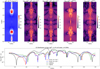 |
Fig. 5 Same as Fig. 4 but for ρH. |
| In the text | |
|
Fig. 6 Time evolution of the flux ratio of helium species relative to the total flux of all species, ϕ(He + He+)/(ϕ(He + He+) + ϕ(H + H+)), at two different locations, z = 1.7 Mm (black line) and z = 1.9 Mm (red line). |
| In the text | |
Current usage metrics show cumulative count of Article Views (full-text article views including HTML views, PDF and ePub downloads, according to the available data) and Abstracts Views on Vision4Press platform.
Data correspond to usage on the plateform after 2015. The current usage metrics is available 48-96 hours after online publication and is updated daily on week days.
Initial download of the metrics may take a while.