| Issue |
A&A
Volume 692, December 2024
|
|
|---|---|---|
| Article Number | A214 | |
| Number of page(s) | 10 | |
| Section | The Sun and the Heliosphere | |
| DOI | https://doi.org/10.1051/0004-6361/202452324 | |
| Published online | 13 December 2024 | |
Estimating the early propagation direction of the coronal mass ejection with DIRECD during the severe event on May 8 and for the follow-up event on June 8, 2024
1
Skolkovo Institute of Science and Technology, Bolshoy Boulevard 30, bld. 1, 121205 Moscow, Russia
2
University of Graz, Institute of Physics, Universitätsplatz 5, 8010 Graz, Austria
3
University of Graz, Kanzelhöhe Observatory for Solar and Environmental Research, Kanzelhöhe 19, 9521 Treffen, Austria
4
University of Zagreb, Faculty of Geodesy, Hvar Observatory, Kaciceva 26, HR-10000 Zagreb, Croatia
5
NorthWest Research Associates, 3380 Mitchell Lane, Boulder, 80301 CO, USA
⋆ Corresponding author; shantanu.jain@skoltech.ru
Received:
20
September
2024
Accepted:
22
October
2024
Context. On May 8, 2024, the solar active region 13664 produced an X-class flare, several M-class flares, and multiple coronal mass ejections (CMEs) directed towards Earth. The initial CME resulted in coronal dimmings, which are characterized by localized reductions in extreme-ultraviolet (EUV) emissions and are indicative of mass loss and expansion during the eruption. On June 8, 2024, after one solar rotation, the same active region produced another eruptive M-class flare that was followed by coronal dimmings that were observed by the Solar Dynamics Observatory (SDO) and the Solar Terrestrial Relations Observatory (STEREO) spacecraft.
Aims. We analyzed the early CME evolution and propagation direction from the expansion of the coronal dimming observed low in the corona using the method called dimming inferred estimation of the CME direction (DIRECD).
Methods. DIRECD derived the key parameters of the early CME propagation from the expansion behavior of the associated coronal dimming at the end of its impulsive phase by generating a 3D CME cone model whose orthogonal projection on the solar sphere matches the dimming geometry. To validate the resulting 3D CME cone, we compared the CME properties derived in the low corona with white-light coronagraph data.
Results. Using DIRECD, we find that the CME on May 8, 2024 expands close to radially, with an inclination angle of 7.7°, an angular width of 70°, and a cone height of 0.81 Rsun, which was derived at the end of the impulsive dimming phase, and for which the CME showed connections to the dimming and still left footprints in the low corona. It was inclined 7.6° north in the meridional plane and 1.1° east in the equatorial plane. The CME on June 8, 2024, after one solar rotation, was inclined by 15.7° from the radial direction, had an angular width of 81°, and had a cone height of 0.89 Rsun. The CME was inclined 6.9° south in the meridional plane and 14.9° west in the equatorial plane. A validation with white-light coronagraph data confirmed the accuracy of the 3D cone by matching the CME characteristics and projections with STEREO-A COR2 observations.
Conclusions. Our study demonstrates that by tracking low coronal signatures such as the coronal dimming expansion in 2D for the May and June 2024 CMEs, we can estimate the 3D CME direction early in the CME evolution. This provides early lead times for mitigating adverse space weather impacts.
Key words: Sun: activity / Sun: corona / Sun: coronal mass ejections (CMEs) / Sun: evolution
© The Authors 2024
 Open Access article, published by EDP Sciences, under the terms of the Creative Commons Attribution License (https://creativecommons.org/licenses/by/4.0), which permits unrestricted use, distribution, and reproduction in any medium, provided the original work is properly cited.
This article is published in open access under the Subscribe to Open model. Subscribe to A&A to support open access publication.
1. Introduction
Coronal mass ejections (CMEs) are the most powerful events in the Solar System. They cause significant disturbance in space weather. These phenomena involve clouds of magnetized plasma that are expelled from the Sun at very high velocities (Michalek et al. 2009; Gopalswamy et al. 2009; Tsurutani & Lakhina 2014; Cheng et al. 2017; Veronig et al. 2018). CMEs can pose a threat to technological systems, as they can disrupt radio transmissions, induce currents in power grids, and lower the orbits of Earth-orbiting satellites (Sandford 1999; Doherty et al. 2004; Baker et al. 2013). Statistical analyses showed that fast CMEs that launched sequentially from the same active region are more geoeffective than isolated CMEs (Vennerstrom et al. 2016; Lugaz et al. 2017; Rodríguez Gómez et al. 2020; Scolini et al. 2020). It is therefore important to detect and study the early evolution of CMEs. Since the early CME evolution is not well observed by coronagraphs due to projection effects (Schwenn et al. 2005) and the early location cannot be known due to the occulation disk, a number of studies have tried to explore whether any CME-related phenomena may give us more insight into the early CME evolution.
Coronal dimmings are one such phenomenon associated with CMEs. he dimmings are regions of reduced extreme ultraviolet (EUV) and X-ray emission in the low corona (Hudson et al. 1996; Sterling & Hudson 1997; Thompson et al. 1998). Numerous studies have explored the strong connection between the initial development of CMEs and coronal dimmings in the lower corona. Some of these investigations examined the relation of coronal dimmings to the mass of a CME (e.g., (Harrison & Lyons 2000; Harrison et al. 2003; Zhukov & Auchère 2004; López et al. 2017), the morphology and early evolution of the CME (Attrill et al. 2006; Qiu & Cheng 2017), and their timing (Miklenic et al. 2011; Ronca et al. 2024). Additionally, various studies have examined the statistical relation between CMEs and coronal dimmings (Bewsher et al. 2008; Reinard & Biesecker 2009; Mason et al. 2016; Krista & Reinard 2017; Aschwanden 2017), which revealed strong correlations between the CME mass and the dimming area, the dimming brightness and the magnetic flux within the dimming region, and between the CME maximum speed and parameters such as the area growth rate, brightness change rate, and magnetic flux rate, along with the mean intensity of the dimmings (Dissauer et al. 2018a, 2019; Chikunova et al. 2020).
Several models exist for determining the CME propagation direction and deflections. One such model is called the graduated cylindrical shell (GCS) model (Thernisien et al. 2006; Thernisien 2011). It is a parametric forward-fitting approach that is used to describe the three-dimensional shape of CMEs based on stereoscopic observations from coronagraphs at heights of up to 20 Rsun. Another method is elliptical tie-pointing (Byrne et al. 2010), which involves tracing the elliptical CME front from multiple viewpoints (e.g., from two spacecraft, such as STEREO-A and STEREO-B) and determining its 3D structure by triangulating the positions of corresponding points in each view. Additionally, geometric triangulation (Liu et al. 2010; Podladchikova et al. 2019) is used to estimate the 3D position of a CME by measuring the same feature in images taken from two different viewpoints and using the angular separation between the spacecraft to infer the 3D position of specific points or features within the CME structure. These and other techniques contribute to understanding CME propagation in space.
(Chikunova et al. 2023) found a link between the dimming morphology and the 3D structure of CMEs, suggesting that dimming observations might also provide insights into early CME evolution. This idea was further explored using the DIRECD method described by Jain et al. (2024) to infer the initial CME propagation direction from coronal dimmings. The DIRECD method focuses on estimating the early-stage CME direction using coronal dimming, while the GCS and other models provide a more detailed 3D structure of CMEs after they are observed by coronagraphs.
We analyze two recent extreme space weather events that occurred on May 8, 2024 and June 8, 2024, when CMEs erupted from the same active region AR3664 (AR3697 after one solar rotation), and we estimate the CME parameters in its early evolution from the associated coronal dimmings using the DIRECD method with further refined selection criteria. The associated flares were listed in the XRT flare catalog (Watanabe et al. 2012) and the publicly available space weather database of notifications, knowledge, information1 (DONKI) catalog. During the May 2024 storms, the agencies reported a variety of impacts, such as satellites that experienced increased drag (Parker & Linares 2024) and strong geomagnetic disturbances in the Earth’s atmosphere (Hayakawa et al. 2024).
2. Event of May 8, 2024
In the early hours of May 8, 2024, a series of eruptions were ejected into interplanetary space from active region 13364 (one of the largest in the current solar cycle). We focus our study to the first CME that erupted at 04:30 UT and was closely followed by three CMEs (see the related video using Jhelioviewer Müller et al. 2017). A total of six CMEs erupted and arrived near Earth on May 10. At around 12:30 UT on May 10, the first CME reached Earth, leading to a significant geomagnetic storm that included auroras as far as 21° latitude (Parker & Linares 2024) and increased ionospheric activity (Spogli et al. 2024). Moreover, around 5000 spacecraft had to adjust their altitude to counteract the effects of a geomagnetic storm (Parker & Linares 2024). The Dst index, which measures the intensity of geomagnetic storms and is primarily linked to the magnetospheric ring current (Gonzalez et al. 1994), peaked at –412 nT (real-time quicklook Dst index) on May 11, 2024, at 03:00 UT. This amplitude was accurately predicted several hours in advance by the StormFocus service2, as shown in the prediction screenshot3. The forecast was based on real-time solar wind and interplanetary magnetic field data provided at the L1 Sun-Earth libration point (Podladchikova & Petrukovich 2012; Podladchikova et al. 2018). This was the largest geomagnetic storm since November 20, 2003, with a peak Dst of –422 nT, and since 1995, no storms have surpassed this intensity. This makes the May 8, 2024, event the second strongest storm of the 21st century.
The first solar eruptions in the early hours of May 8, 2024 (Hayakawa et al. 2024) were followed by coronal dimming that was observed on the solar surface by the SDO (Pesnell et al. 2012) and the STEREO (Kaiser et al. 2008) spacecraft. In this study, we use the information from these dimmings observed by SDO to estimate CME properties such as angular width, inclination from the radial direction, and height, where the CME connects to the dimming, and we relate the properties with white-light coronagraph data.
2.1. Dimming detection for the May 8, 2024, event
We detected coronal dimmings using the region-growing algorithm described by Dissauer et al. (2018a,b, 2019) from a series of 193 Å images (4096 × 4096 pixel) from the Atmospheric Imaging Assembly (AIA) (Lemen et al. 2012) telescopes on board the SDO spacecraft with a one-minute cadence within the time range 04:30–06:30 UT. We took a pre-eruption base map (30 minutes prior to the start time, at 04:00 UT) and applied differential rotation correction to the same reference time (04:00 UT) for all the images in the sequence to compare the drop in EUV intensity with respect to the pre-eruptive coronal state. The SDO/AIA images were processed and calibrated using the aiapy programs in the SunPy library (The SunPy Community et al. 2020). We further cropped the images around the eruption source determined by visual analysis from the JHelioviewer client, focusing on a region of 1000 × 1000 arcseconds. The dimming detection algorithm was applied to logarithmic base-ratio images using the automatic thresholding technique (Dissauer et al. 2018b). We extracted the darkest 30% of pixels with a logarithmic threshold of −0.15 and applied median filtering with a box of 10 × 10 pixels to reduce noise in the images. The detected dimming pixels were saved in a cumulative map at each time step, and the area of the dimming expansion was calculated using the method presented in Chikunova et al. (2023), which allowed us to estimate the surface area of a sphere for each pixel4.
Figure 1 presents the evolution of the derived dimming area At (top panel) and its time derivative dA/dt (bottom panel) over a duration of 2 hours. We determined the end of the impulsive phase to be 05:43 UT, defined by the criteria in Dissauer et al. (2018b), where the end of the impulsive phase occurs when the change rate of the dimming area dA/dt falls below 15% of its maximum value.
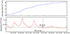 |
Fig. 1. Expansion of the dimming area At (top panel) and its time derivative dAt/dt (bottom panel) over 2 hours for the 8 May 2024 event. The end of the impulsive phase (indicated by the vertical dashed line) is defined as the time when the derivative of the dimming area curve, dAt/dt, declined to 15% of its maximum value. |
Figure 2 shows the timing map of the dimming evolution. Each dimming pixel is colored according to the time it was first detected relative to the event start time. For DIRECD, we used the dimming map at the end of the impulsive phase (panel c).
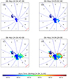 |
Fig. 2. Dimming evolution for the May 8, 2024 CME at four different time steps: (a) 15 minutes before the maximum of the impulsive phase (04:47 UT), (b) at the maximum of the impulsive phase (05:02 UT), (c) at the end of the impulsive phase (05:43 UT), and (d) 2 hours after the start. The blue lines indicate 12 angular sectors and the color bar shows the first detection of each dimming pixel. |
2.2. Application of DIRECD to the May 2024 event
The DIRECD method for estimating the early propagation of CMEs from the expansion of dimmings involves the following main steps. First, we estimated the dominant direction of the dimming extent based on the evolution of the dimming area (Fig. 2). Second, using the derived dominant direction of the dimming evolution on the solar sphere, we solved an inverse problem to reconstruct an ensemble of 3D CME cones at different heights, widths, and deflections from the radial propagation. Third, we searched for the CME parameters for which the 3D cone orthogonal projections onto the solar sphere would match the geometry of the dimming at the end of its impulsive phase best.
Figure 3a shows the area distribution curve for each sector at the end of the dimming impulsive phase. We defined the dominant dimming direction in the middle of the sector with the largest dimming area (sector 10). Further, we chose two dimming edges that are farthest from the source, which is the centroid of the detected dimming. One edge is in sector 10 along the dominant dimming direction, and the other edge is in sector 3, as shown in Fig. 3b. We then constructed two 3D lines from the Sun center to the two dimming edges. These lines form the boundaries of an ensemble of 3D cones, whose projections align with the dimming geometry. We then generated an ensemble of 3D CME cones where every cone was defined by its unique height, inclination angle, and width, maintaining a connection to the dimming. Given the relation between CMEs and dimmings, the CME cone naturally tilts in the dominant dimming direction, aligning the axis of the smaller cone with this direction. As the inclination angle increases, the length of the main cone axis shortens. In our approach, we fixed the small cone axis while allowing the larger cone axis to vary. This means that the identification of the dominant dimming direction is a critical and advantageous part of the method.
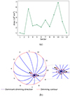 |
Fig. 3. Dominant direction of the dimming expansion at the end of the impulsive phase for May 8, 2024. Top: Dimming area in the different sectors (shown in the bottom panels in blue), revealing its maximum extent in sector 10. Bottom: Cumulative dimming pixel mask outlined in gray with red contours. The blue lines indicate the 12 sectors. The dashed purple line gives the sector of the dominant dimming development. The small black dots show the dimming edges at the farthest edges from the source (one of them is in the sector of the dominant dimming direction and the other is in sector 3), which were used to generate the 3D CME cones at different heights, associated widths, and inclination angles. |
Figure A.1 shows an ensemble of 20 such cones with heights ranging from 0.15 to 2.08 Rsun, angular widths varying from 132.6° to 49.8°, and changing inclination angles of 24.4°–5.2° (Cols. 1 and 3) and their orthogonal projections onto the solar sphere (Cols. 2 and 4). Columns 1 and 3 depict the top view to better show the reconstructed cones, and Columns 2 and 4 show the face-on view. The heights in the constructed ensemble of cones are a representation of the heights at which the CME is assumed to leave footprints in the low corona and remains connected to the dimming. Figure A.1 shows that the cone projections are required to be wider for smaller heights and become narrower for larger heights, but only marginally so, to fit the observed dimming extent.
To quantify the dynamics of the cone projections and to choose the 3D CME cone that matches the dimming geometry best, we first considered the consecutive differences of the cone projection areas AΔhi, j for every cone height (hi, hj),
The evolution of AΔh1, 2 is shown in Fig. 4 (blue line, top panel) and indicates the shrinking projection areas. We selected the cone that fit the dimming best at the point of the strongest shrinking in the projection areas, where the cone projections remain sensitive to changes in the cone parameters. This is estimated to be at 5% (vertical dashed line) of the blue line peak. In the current case, this corresponds to a 3D CME cone with a height range of 0.61 Rsun–0.81 Rsun, corresponding to a width range of 79.0°–69.8° and to inclination angles of 9.0°–7.7°.
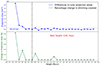 |
Fig. 4. Consecutive differences of the cone projection areas AΔh1, 2 defined by Eq. (1) (blue line, top panel) and the percentage of the relative change in the dimming area inside the projection area for consecutive cones (green line, bottom panel) for the May 8, 2024, event. The vertical dashed line indicates the step (associated with a cone height of 0.81 Rsun, a width of 69.8°, and an inclination angle of 7.7°) where the consecutive differences (blue line) reach 5% of the maximum of the cone projection area and just before the increase in percentage of the relative change in the dimming area within the projections (green line). |
Additionally, we required the majority of the dimming area to be inside the cone projection by considering the percentage of the relative change in the dimming area inside the projection area for the consecutive cones (Fig. 4, green line, bottom panel), defined as

where Ad and Ap are the dimming and projection area, respectively. Sk is the area of the dimming inside the projection area for a cone height hk, and Sk + 1 is the area of the dimming inside the projection area for the consecutive cone height hk + 1.
We chose the 3D CME cone that matched the dimming best just before the abrupt increase in the criteria above, which is in range of the initial choice of the CME parameters early in its evolution (see the details in Appendix B). Figure 5a shows the resulting best-fit 3D CME cone (green) with a height of 0.81 Rsun, a width of 69.8°, and an inclination angle of 7.7°, and its orthogonal projections (green dots) together with the dimming boundaries at the end of its impulsive phase.
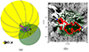 |
Fig. 5. Application of the DIRECD method to relate the expansion of coronal dimming to the early CME propagation. (a) Best fit DIRECD cone with the dimming outlined by magenta boundaries. Points A and B mark the largest north and south dimming extent. The best-fit green cone has a height of 0.81 Rsun, a width of 69.8°, and an inclination angle of 7.7°. The green dots indicate the orthogonal projections of the CME cone onto the solar surface. We require an edge of the cone base to be orthogonally projected to points A and B to match the dimming extent. (b) Dimming detection: 193 Å SDO/AIA base-difference image together with the boundary of the identified dimming region (red) at the end of the impulsive phase at 05:43 UT. Points A and B mark the largest north and south dimming extent. |
The height of 0.81 Rsun here indicates the height up to which the CME is assumed to leave footprints in the low corona and remains connected to the dimming (Jain et al. 2024). Figure 5b shows a 193 Å SDO/AIA base-difference image, along with the boundary of the identified dimming region (in red) at the end of the impulsive phase. The source is marked by point C. The largest extent of the dimming in the north and south direction is indicated by points A and B, respectively.
Figure 6 shows the best-fit cone inclination within the radial and meridional planes. The red meridional plane intersects the center O of the Sun, source C on the solar surface, and the North Pole. The green plane passes through point C and is aligned parallel to the equatorial plane of the Sun.
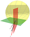 |
Fig. 6. Projection of the CME direction onto the meridional (red) and equatorial (green) planes. The radial direction lies in the red meridional plane by definition (along the line CC′), and the dashed red line shows its projection onto the equatorial plane (CC″). The dashed black line gives the projection of the central cone axis CP (the CME direction in 3D) to the meridional plane (CP′), and the equatorial plane (CP″). |
We obtained that the event on May 8, 2024 was inclined north from the radial direction by 7.6° (i.e., in the meridional plane) and east by 1.1° (in the equatorial plane).
To connect the structures of the eruption in the EUV with white-light coronagraph data, Figure 7 shows line-of-sight (LOS) projections of the DIRECD cone extrapolated to 6 Rsun at 05:38 UT (panel a), 05:53 UT (panel b), 08:53 UT (panel c), and 09:53 UT(panel d), capturing the moment when the CME was visible in STEREO-A COR2.
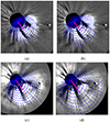 |
Fig. 7. Line-of-sight projections of the DIRECD cone (blue mesh) extended to (a) 6 Rsun at 05:38 UT, (b) 7 Rsun at 05:53 UT, (c) 10 Rsun at 08:53 UT, and (d) 12 Rsun at 09:53 UT plotted on STEREO-A COR2 images. The pink line represents LOS projections of the central cone axes. |
The pink line shows the LOS projections of the central axis for the extended cones, pointing toward the center of the CME bubble. Fig. 7 shows that the central cone line is closely aligned with the inner parts of the CME bubble, whereas the LOS projections of the extended 3D cones closely match the edge of the CME structure that is observed at different time steps in COR2. This correspondence indicates that the connections between the dimming and CME expansion are established by the end of the impulsive dimming phase. Analysis of the dimming evolution allowed us to extract key CME parameters early in its development, such as the 3D propagation direction and angular width. They revealed a subsequent self-similar expansion. This finding is consistent with the studies by Chikunova et al. (2023) and Jain et al. (2024), which demonstrated that the dimming morphology closely reflects the inner part of 3D GCS CME reconstructions where both the DIRECD CME cone and the GCS croissant were reconstructed at the same time at the end of the impulsive dimming phase (the CME bubble was already seen in coronagraphs at this time). These results reinforce the idea that the extent of the dimming is related to the CME propagation and leaves distinct footprints in the low corona that can be observed up to a certain height, as indicated by the parameters derived from DIRECD. These resemblances imply that the best-fit cone from the DIRECD method can be used not only to link the 2D dimming with the 3D CME bubble to provide an estimate of the early CME direction, but also to provide further information for improving the estimations of the GCS parameters using dimmings are signatures of the CME propagation in the low corona. This can provide us with a comprehensive picture of the CME evolution in the low corona (using DIRECD) to higher up in the heliosphere (using GCS or similar reconstructions).
3. Event of June 8, 2024
On June 8, 2024, at 00:49 UT, active region AR3697 (previously AR3664) produced yet another intense solar flare (M9.7) that ionized the top of the Earth’s atmosphere and caused shortwave radio blackouts across the western Pacific Ocean. However, its impact on Earth was weaker, and the associated CME did not cause a geomagnetic storm. The event was accompanied by a huge coronal dimming as observed from SDO and STEREO-A. For SDO, part of the observed dimming was very close to the limb and part of the eruption was off-limb. For STEREO-A, the dimming was observed on-disk, but also very close to the limb. Applying DIRECD, we used the STEREO-A on-disk dimming information.
We used a set of STEREO/EUVI (Extreme Ultraviolet Imager) images within the time range 00:30–03:30 UT, taking the first map as the base map (00:30 UT), and we applied the same calibration steps and dimming detection as for the May 2024 event. In this way, we created a series of base-difference images showing the absolute intensity drop with respect to the pre-eruption state, with a threshold of −40 DN (chosen based on the dimming development at different stages), and we extracted the top 30% of darkest pixels as seed pixels for the region-growing algorithm.
Figure 8 shows the dimming area evolution over the 3 hours of interest. The end of the impulsive phase (15% of maximum) is at 02:22:30 UT. The timing map shows that the dimming seems to expand radially from the source in all sectors (Fig. 9). We note that there is a partial off-limb dimming at the end of our three-hour time period (panel d), but we used the dimming map at the end of impulsive phase for DIRECD (panel c), where the dimming expansion is on-disk. As shown in Fig. 10a, the dominant dimming direction is in sector 10. This is illustrated by the dotted line in Fig. 10b along with the farthest dimming edges from the source (edge 1 between sectors 6 and 7, and edge 2 in sector 11), which we extended into 3D space to constrain the 3D-generated CME cones.
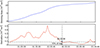 |
Fig. 8. Expansion of the dimming area At (top panel) and its time derivative dAt/dt (bottom panel) over 3 hours for the June 8, 2024, event. The end of the impulsive phase is defined as the time when the derivative of the dimming area curve, dAt/dt, declined to 15% of its maximum value. |
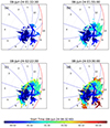 |
Fig. 9. Dimming evolution for the June 8, 2024 CME at (a) 22 minutes before the maximum of the impulsive phase (01:32 UT), (b) at the maximum of the impulsive phase (01:55 UT), (c) at the end of the impulsive phase (02:22 UT), and (d) 3 hours after the start time of our analysis. The blue lines indicate 12 angular sectors and the color bar shows the first dectection of each dimming pixel. |
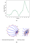 |
Fig. 10. Dominant direction of the dimming expansion at the end of the impulsive phase for June 8, 2024. Top: Dimming area in the different sectors (shown in the bottom panels), showing its maximum in sector 10. Bottom: Cumulative dimming pixel mask outlined in gray with red contours. The blue lines indicate the 12 sectors. The dashed purple line gives the sector of the dominant dimming development. The small black dots show the dimming edges at the farthest edges from the source (one of them in sector 11 and other in sector 6), which were used to generate the 3D CME cones at different heights, associated widths, and inclination angles. |
Figure A.2 shows an ensemble of 20 cones with heights ranging from 0.12 to 2.03 Rsun, angular widths of 136.8° −62.7°, and changing inclination angles from 52.5° to 11.1° (Cols. 1 and 3) and their orthogonal projections onto the solar sphere (Cols. 2 and 4). To determine the 3D CME cone that matches the dimming geometry best, we used the same criteria as for the May 8, 2024, event, as shown in Fig. 11.
We obtained that the best-fit 3D CME cone has a height of 0.89 Rsun (where the CME still connects to the dimming), a width of 81°, and inclination angle of 15.7° (Fig. 12a). Figure 12b shows a 195 Å STEREO-A EUVI base-difference image, along with the boundary of the identified dimming region (in red) at the end of the impulsive phase. The source is marked by point C. The largest extent of the dimming in the north and south direction is indicated by points A and B, respectively.
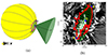 |
Fig. 12. Application of the DIRECD method to relate the expansion of coronal dimming to the early CME propagation for June event. (a) Best fit cone outlined by magenta boundaries. The best-fit green cone has a height of 0.89 Rsun, a width of 81°, and inclination angle of 15.7°. The green dots indicate the orthogonal projections of the CME cone onto the solar surface. We require an edge of the cone base to be orthogonally projected to points A and B to match the dimming extent. (b) Dimming detection: 195Å EUVI/STEREO-A base-difference image together with the boundary of the identified dimming region (red) at the end of impulsive phase at 02:22 UT. Points A and B mark the largest north and south dimming extent. |
Figure 13 shows the best-fit cone inclination within the radial and meridional planes. We obtained that the event on June 8, 2024 was inclined south from the radial direction by 6.9° (i.e., in the meridional plane) and west by 14.9° (in the equatorial plane).
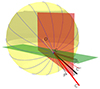 |
Fig. 13. Same as Fig. 6, but for June 8, 2024. The best-fit cone is inclined 6.9° south (meridional plane) and 14.9° west (equatorial plane). |
The best-fit cone extrapolated to 7 Rsun and 9 Rsun (keeping width and the inclination angle constant), and its LOS projections are plotted on both STEREO-A EUVI (02:22 UT) and COR2 (03:07 UT, 04:07 UT) images (Fig. 14). The LOS projections of the central cone axes are directed at the center of the bubble, which is captured by the core dimming. This confirms that dimmings serve as reliable indicators for deriving key CME parameters early in its development. It is to be noted that the secondary dimming regions extend farther north and south than the initial core dimming. They correspond to the outer edges of CME bubble white-light signature as observed in STEREO-A and were not fit within the DIRECD cone.
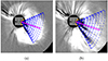 |
Fig. 14. Line-of-sight projections of the DIRECD cone extended to (a) 7 Rsun (blue mesh) on top of a composite of 195 Å EUVI (02:22 UT) and COR2 (03:07 UT), and to (b) 9 Rsun (blue mesh) on top of a composite of 195 Å EUVI (02:22 UT) and COR2 (04:07 UT). The pink line represents LOS projections of the central cone axes, and the orange arrows show the direction of bubble from the secondary dimming regions. |
Remote dimming regions extend farther north and south beyond the central dimming area. These regions, indicated by orange arrows in Fig. 14, are not accounted for in the DIRECD model, but are aligned with the outer boundaries of the CME bubble white-light signature, as seen in the STEREO-A COR2 coronagraph image.
4. Conclusions
We estimated the early evolution and propagation of the CME direction with DIRECD for the severe event on May 8 and the follow-up event on June 8, 2024, from the expansion of the coronal dimming. It was shown that the link between the dimming and the CME expansion was established by the end of the impulsive dimming phase, which allowed us to determine the key CME characteristics during the early CME evolution.
Using SDO/AIA 193 Å images for the May 8, 2024, event, we found that the CME expands close to radial, with an inclination angle of 7.7°, an angular width of 69.8°, and a cone with a height of 0.81 Rsun, which was derived at the end of the impulsive dimming phase, and for which the CME showed connections to the dimming and still left footprints in the low corona. The CME was inclined north by 7.6° in the meridional plane and east by 1.1° in the equatorial plane. For the follow-up event on June 8, 2024, we used STEREO/EUVI images for the on-disk dimming and determined that the CME was inclined on 15.7°, had an angular width of 81°, and a height of 0.89 Rsun, for which the dimming was still connected to the CME. The CME was inclined south by 6.9° in the meridional plane and west by 14.9° in the equatorial plane.
Furthermore, we validated the 3D CME cone derived by DIRECD by correlating the CME properties derived in the low corona with white-light coronagraph data. We showed that for both events, the extended 3D CME cones, with the key parameters inferred from the EUV coronal dimmings, closely match the shape and edges of the CME structures that were simultaneously observed in the coronagraph, and no CME deflection was observed up to the edge of the STEREO-A field of view. By linking the expanding dimming with the initial stages of the CME development, this approach underscores that coronal dimmings are valuable indicators of the early CME evolution. It also suggests that the DIRECD method can be used not only to correlate 2D dimming with the 3D CME bubble, but also to enhance GCS reconstructions with additional information about the early CME propagation direction in the low corona.
The findings and outcomes of this study offer valuable insights into early CME evolution inferred from the coronal dimmings in the low corona, and the DIRECD method proved to be efficient in estimating the initial CME propagation direction and early CME parameters. Moreover, forecasting space weather involves using simulations such as EUHFORIA (Pomoell & Poedts 2018) to model the behavior of CMEs, for instance, with the cone model, as they move through the heliosphere and approach Earth. For these forecasts to be reliable, the models must incorporate the most precise parameters available. A key parameter in this process is the CME propagation direction, defined by the insertion point coordinates, that is, longitude and latitude, at approximately 0.1 AU, as done in EUHFORIA. The DIRECD method could improve the accuracy of these key parameters at 0.1 AU, which would lead to more reliable predictions for space weather events.
Acknowledgments
S.J., T.P. acknowledge support by the Russian Science Foundation under the project 23-22-00242, https://rscf.ru/en/project/23-22-00242/. G.C. and M.D. acknowledge the support by the Croatian Science Foundation under the project IP-2020-02-9893 (ICOHOSS). A.V. and M.D. acknowledge the support from the Austrian-Croatian Bilateral Scientific Project “Analysis of solar eruptive phenomena from cradle to grave”. SDO data is courtesy of NASA/SDO and the AIA, and HMI science teams. The STEREO/SECCHI data are produced by an international consortium of the Naval Research Laboratory (USA), Lockheed Martin Solar and Astrophysics Lab (USA), NASA Goddard Space Flight centre (USA), Rutherford Appleton Laboratory (UK), University of Birmingham (UK), Max-Planck- Institut für Sonnenforschung (Germany), Centre Spatiale de Liége (Belgium), Institut d’Optique Théorique et Appliquée (France), and Institut d’Astrophysique Spatiale (France). We thank the referee for valuable comments on this study.
References
- Aschwanden, M. J. 2017, ApJ, 847, 27 [NASA ADS] [CrossRef] [Google Scholar]
- Attrill, G., Nakwacki, M. S., Harra, L. K., et al. 2006, Sol. Phys., 238, 117 [Google Scholar]
- Baker, D. N., Li, X., Pulkkinen, A., et al. 2013, Space Weather, 11, 585 [NASA ADS] [CrossRef] [Google Scholar]
- Bewsher, D., Harrison, R. A., & Brown, D. S. 2008, A&A, 478, 897 [NASA ADS] [CrossRef] [EDP Sciences] [Google Scholar]
- Byrne, J. P., Maloney, S. A., McAteer, R. T. J., Refojo, J. M., & Gallagher, P. T. 2010, Nat. Commun., 1, 74 [NASA ADS] [CrossRef] [Google Scholar]
- Cheng, X., Guo, Y., & Ding, M. 2017, Sci. China Earth Sci., 60, 1383 [Google Scholar]
- Chikunova, G., Dissauer, K., Podladchikova, T., & Veronig, A. M. 2020, ApJ, 896, 17 [NASA ADS] [CrossRef] [Google Scholar]
- Chikunova, G., Podladchikova, T., Dissauer, K., et al. 2023, A&A, 678, A166 [NASA ADS] [CrossRef] [EDP Sciences] [Google Scholar]
- Dissauer, K., Veronig, A. M., Temmer, M., Podladchikova, T., & Vanninathan, K. 2018a, ApJ, 863, 169 [NASA ADS] [CrossRef] [Google Scholar]
- Dissauer, K., Veronig, A. M., Temmer, M., Podladchikova, T., & Vanninathan, K. 2018b, ApJ, 855, 137 [NASA ADS] [CrossRef] [Google Scholar]
- Dissauer, K., Veronig, A. M., Temmer, M., & Podladchikova, T. 2019, ApJ, 874, 123 [NASA ADS] [CrossRef] [Google Scholar]
- Doherty, P., Coster, A. J., & Murtagh, W. 2004, GPS Solutions, 8, 267 [NASA ADS] [CrossRef] [Google Scholar]
- Gonzalez, W. D., Joselyn, J. A., Kamide, Y., et al. 1994, J. Geophys. Res., 99, 5771 [NASA ADS] [CrossRef] [Google Scholar]
- Gopalswamy, N., Yashiro, S., Michalek, G., et al. 2009, Earth Moon Planets, 104, 295 [NASA ADS] [CrossRef] [Google Scholar]
- Harrison, R. A., & Lyons, M. 2000, A&A, 358, 1097 [NASA ADS] [Google Scholar]
- Harrison, R. A., Bryans, P., Simnett, G. M., & Lyons, M. 2003, A&A, 400, 1071 [NASA ADS] [CrossRef] [EDP Sciences] [Google Scholar]
- Hayakawa, H., Ebihara, Y., Mishev, A., et al. 2024, ApJ, accepted [arXiv:2407.07665] [Google Scholar]
- Hudson, H. S., Acton, L. W., & Freeland, S. L. 1996, ApJ, 470, 629 [CrossRef] [Google Scholar]
- Jain, S., Podladchikova, T., Chikunova, G., Dissauer, K., & Veronig, A. M. 2024, A&A, 683, A15 [NASA ADS] [CrossRef] [EDP Sciences] [Google Scholar]
- Kaiser, M. L., Kucera, T., Davila, J., et al. 2008, Space Sci. Rev., 136, 5 [NASA ADS] [CrossRef] [Google Scholar]
- Krista, L. D., & Reinard, A. A. 2017, ApJ, 839, 50 [NASA ADS] [CrossRef] [Google Scholar]
- Lemen, J. R., Title, A. M., Akin, D. J., et al. 2012, Sol. Phys., 275, 17 [Google Scholar]
- Liu, Y., Thernisien, A., Luhmann, J. G., et al. 2010, ApJ, 722, 1762 [Google Scholar]
- López, F. M., Hebe Cremades, M., Nuevo, F. A., Balmaceda, L. A., & Vásquez, A. M. 2017, Sol. Phys., 292, 6 [CrossRef] [Google Scholar]
- Lugaz, N., Temmer, M., Wang, Y., & Farrugia, C. J. 2017, Sol. Phys., 292, 1 [NASA ADS] [CrossRef] [Google Scholar]
- Mason, J. P., Woods, T. N., Webb, D. F., et al. 2016, ApJ, 830, 20 [NASA ADS] [CrossRef] [Google Scholar]
- Michalek, G., Gopalswamy, N., & Yashiro, S. 2009, Sol. Phys., 260, 401 [NASA ADS] [CrossRef] [Google Scholar]
- Miklenic, C., Veronig, A. M., Temmer, M., Möstl, C., & Biernat, H. K. 2011, Sol. Phys., 273, 125 [NASA ADS] [CrossRef] [Google Scholar]
- Müller, D., Nicula, B., Felix, S., et al. 2017, A&A, 606, A10 [Google Scholar]
- Parker, W. E., & Linares, R. 2024, J. Spacecr. Rockets, 61, 1412 [NASA ADS] [CrossRef] [Google Scholar]
- Pesnell, W. D., Thompson, B. J., & Chamberlin, P. 2012, The Solar Dynamics Observatory (SDO) (Springer) [Google Scholar]
- Podladchikova, T. V., & Petrukovich, A. A. 2012, Space Weather, 10, S07001 [NASA ADS] [CrossRef] [Google Scholar]
- Podladchikova, T., Petrukovich, A., & Yermolaev, Y. 2018, J. Space Weather Space Clim., 8, A22 [NASA ADS] [CrossRef] [EDP Sciences] [Google Scholar]
- Podladchikova, T., Veronig, A. M., Dissauer, K., Temmer, M., & Podladchikova, O. 2019, ApJ, 877, 68 [NASA ADS] [CrossRef] [Google Scholar]
- Pomoell, J., & Poedts, S. 2018, J. Space Weather Space Clim., 8, A35 [NASA ADS] [CrossRef] [EDP Sciences] [Google Scholar]
- Qiu, J., & Cheng, J. 2017, ApJ, 838, L6 [NASA ADS] [CrossRef] [Google Scholar]
- Reinard, A. A., & Biesecker, D. A. 2009, ApJ, 705, 914 [Google Scholar]
- Rodríguez Gómez, J. M., Podladchikova, T., Veronig, A., et al. 2020, ApJ, 899, 47 [CrossRef] [Google Scholar]
- Ronca, G. M., Chikunova, G., Dissauer, K., Podladchikova, T., & Veronig, A. M. 2024, A&A, 691, A195 [NASA ADS] [CrossRef] [EDP Sciences] [Google Scholar]
- Sandford, W. H. 1999, J. Navig., 52, 42 [NASA ADS] [CrossRef] [Google Scholar]
- Schwenn, R., dal Lago, A., Huttunen, E., & Gonzalez, W. D. 2005, Ann. Geophys., 23, 1033 [Google Scholar]
- Scolini, C., Chané, E., Temmer, M., et al. 2020, ApJS, 247, 21 [Google Scholar]
- Spogli, L., Alberti, T., Bagiacchi, P., et al. 2024, Ann. Geophys., 67, PA218 [CrossRef] [Google Scholar]
- Sterling, A. C., & Hudson, H. S. 1997, ApJ, 491, L55 [Google Scholar]
- The SunPy Community, Barnes, W. T., Bobra, M. G., et al. 2020, ApJ, 890, 68 [NASA ADS] [CrossRef] [Google Scholar]
- Thernisien, A. 2011, ApJS, 194, 33 [Google Scholar]
- Thernisien, A. F. R., Howard, R. A., & Vourlidas, A. 2006, ApJ, 652, 763 [Google Scholar]
- Thompson, B. J., Plunkett, S. P., Gurman, J. B., et al. 1998, Geophys. Res. Lett., 25, 2465 [Google Scholar]
- Tsurutani, B. T., & Lakhina, G. S. 2014, Geophys. Res. Lett., 41, 287 [NASA ADS] [CrossRef] [Google Scholar]
- Vennerstrom, S., Lefevre, L., Dumbović, M., et al. 2016, Sol. Phys., 291, 1447 [NASA ADS] [CrossRef] [Google Scholar]
- Veronig, A. M., Podladchikova, T., Dissauer, K., et al. 2018, ApJ, 868, 107 [NASA ADS] [CrossRef] [Google Scholar]
- Watanabe, K., Masuda, S., & Segawa, T. 2012, Sol. Phys., 279, 317 [NASA ADS] [CrossRef] [Google Scholar]
- Zhukov, A. N., & Auchère, F. 2004, A&A, 427, 705 [NASA ADS] [CrossRef] [EDP Sciences] [Google Scholar]
Appendix A: Ensemble of cones
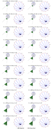 |
Fig. A.1. 3D CME cones at heights of 0.15–2.08 Rsun with widths of 132.6–49.8° and inclination angles of 24.4–5.2° for 8 May 2024 (columns 1 and 3), and their orthogonal projections onto the solar sphere (columns 2 and 4) bounded by the dimming edges. |
Appendix B: Percentage of relative change of the dimming area inside the projection for the consecutive cones
In this section we present a detailed explanation of the criterion used to derive the 3D CME cone, which matches best to the dimming geometry, presented by Eq. 2.
With increase in the cone height, Eq. 2 is monotonically decreasing, which means that denominator Sk decreases for each next step, and Sk < Sk + 1.
Let us consider the introduced criterion at two consecutive steps,
As follows from Eq. B.1, a value of each further shrinking of dimming area inside the projection also decreases, so Sk − Sk + 1 < Sk − 1 − Sk. This indicates the removal of insignificant or possibly random outer fragments of the dimming, which may not be in direct contact with the main dimming area (such as isolated islands). As also follows from Eq. B.1, the ratio of the further shrinking of the dimming area inside the projection to the previous one is smaller than the ratio of the areas inside the projections (Eq. B.2):
However, with a further increase of the cone height, a situation may change sharply, and the sign at a step k0 + 1 is changed to the opposite one:
or
The non-equality in Eq. B.3 changes the sign, as on the step k0 + 1 the area of dimming inside the projection Sk0 + 1 decreased more than on a previous steps. This leads to a strong increase of the numerator of ratio  which is even more, than the ratio of just areas.
The sharp decrease in the dimming area inside the projection is due to a significant increase in the area of contact between the projection perimeter and the selected dimming at step k0 + 1 compared to the previous steps. A further increase in height and a corresponding reduction in projection obviously leads to an undue reduction in the dimming area and distortion of the results. Therefore, we use condition B.3 as a criterion determining the choice of the best-fit 3D cone and associated CME parameters.
All Figures
|
Fig. 1. Expansion of the dimming area At (top panel) and its time derivative dAt/dt (bottom panel) over 2 hours for the 8 May 2024 event. The end of the impulsive phase (indicated by the vertical dashed line) is defined as the time when the derivative of the dimming area curve, dAt/dt, declined to 15% of its maximum value. |
| In the text | |
|
Fig. 2. Dimming evolution for the May 8, 2024 CME at four different time steps: (a) 15 minutes before the maximum of the impulsive phase (04:47 UT), (b) at the maximum of the impulsive phase (05:02 UT), (c) at the end of the impulsive phase (05:43 UT), and (d) 2 hours after the start. The blue lines indicate 12 angular sectors and the color bar shows the first detection of each dimming pixel. |
| In the text | |
|
Fig. 3. Dominant direction of the dimming expansion at the end of the impulsive phase for May 8, 2024. Top: Dimming area in the different sectors (shown in the bottom panels in blue), revealing its maximum extent in sector 10. Bottom: Cumulative dimming pixel mask outlined in gray with red contours. The blue lines indicate the 12 sectors. The dashed purple line gives the sector of the dominant dimming development. The small black dots show the dimming edges at the farthest edges from the source (one of them is in the sector of the dominant dimming direction and the other is in sector 3), which were used to generate the 3D CME cones at different heights, associated widths, and inclination angles. |
| In the text | |
|
Fig. 4. Consecutive differences of the cone projection areas AΔh1, 2 defined by Eq. (1) (blue line, top panel) and the percentage of the relative change in the dimming area inside the projection area for consecutive cones (green line, bottom panel) for the May 8, 2024, event. The vertical dashed line indicates the step (associated with a cone height of 0.81 Rsun, a width of 69.8°, and an inclination angle of 7.7°) where the consecutive differences (blue line) reach 5% of the maximum of the cone projection area and just before the increase in percentage of the relative change in the dimming area within the projections (green line). |
| In the text | |
|
Fig. 5. Application of the DIRECD method to relate the expansion of coronal dimming to the early CME propagation. (a) Best fit DIRECD cone with the dimming outlined by magenta boundaries. Points A and B mark the largest north and south dimming extent. The best-fit green cone has a height of 0.81 Rsun, a width of 69.8°, and an inclination angle of 7.7°. The green dots indicate the orthogonal projections of the CME cone onto the solar surface. We require an edge of the cone base to be orthogonally projected to points A and B to match the dimming extent. (b) Dimming detection: 193 Å SDO/AIA base-difference image together with the boundary of the identified dimming region (red) at the end of the impulsive phase at 05:43 UT. Points A and B mark the largest north and south dimming extent. |
| In the text | |
|
Fig. 6. Projection of the CME direction onto the meridional (red) and equatorial (green) planes. The radial direction lies in the red meridional plane by definition (along the line CC′), and the dashed red line shows its projection onto the equatorial plane (CC″). The dashed black line gives the projection of the central cone axis CP (the CME direction in 3D) to the meridional plane (CP′), and the equatorial plane (CP″). |
| In the text | |
|
Fig. 7. Line-of-sight projections of the DIRECD cone (blue mesh) extended to (a) 6 Rsun at 05:38 UT, (b) 7 Rsun at 05:53 UT, (c) 10 Rsun at 08:53 UT, and (d) 12 Rsun at 09:53 UT plotted on STEREO-A COR2 images. The pink line represents LOS projections of the central cone axes. |
| In the text | |
|
Fig. 8. Expansion of the dimming area At (top panel) and its time derivative dAt/dt (bottom panel) over 3 hours for the June 8, 2024, event. The end of the impulsive phase is defined as the time when the derivative of the dimming area curve, dAt/dt, declined to 15% of its maximum value. |
| In the text | |
|
Fig. 9. Dimming evolution for the June 8, 2024 CME at (a) 22 minutes before the maximum of the impulsive phase (01:32 UT), (b) at the maximum of the impulsive phase (01:55 UT), (c) at the end of the impulsive phase (02:22 UT), and (d) 3 hours after the start time of our analysis. The blue lines indicate 12 angular sectors and the color bar shows the first dectection of each dimming pixel. |
| In the text | |
|
Fig. 10. Dominant direction of the dimming expansion at the end of the impulsive phase for June 8, 2024. Top: Dimming area in the different sectors (shown in the bottom panels), showing its maximum in sector 10. Bottom: Cumulative dimming pixel mask outlined in gray with red contours. The blue lines indicate the 12 sectors. The dashed purple line gives the sector of the dominant dimming development. The small black dots show the dimming edges at the farthest edges from the source (one of them in sector 11 and other in sector 6), which were used to generate the 3D CME cones at different heights, associated widths, and inclination angles. |
| In the text | |
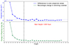 |
Fig. 11. Same as Fig. 4, but for June 8, 2024. |
| In the text | |
|
Fig. 12. Application of the DIRECD method to relate the expansion of coronal dimming to the early CME propagation for June event. (a) Best fit cone outlined by magenta boundaries. The best-fit green cone has a height of 0.89 Rsun, a width of 81°, and inclination angle of 15.7°. The green dots indicate the orthogonal projections of the CME cone onto the solar surface. We require an edge of the cone base to be orthogonally projected to points A and B to match the dimming extent. (b) Dimming detection: 195Å EUVI/STEREO-A base-difference image together with the boundary of the identified dimming region (red) at the end of impulsive phase at 02:22 UT. Points A and B mark the largest north and south dimming extent. |
| In the text | |
|
Fig. 13. Same as Fig. 6, but for June 8, 2024. The best-fit cone is inclined 6.9° south (meridional plane) and 14.9° west (equatorial plane). |
| In the text | |
|
Fig. 14. Line-of-sight projections of the DIRECD cone extended to (a) 7 Rsun (blue mesh) on top of a composite of 195 Å EUVI (02:22 UT) and COR2 (03:07 UT), and to (b) 9 Rsun (blue mesh) on top of a composite of 195 Å EUVI (02:22 UT) and COR2 (04:07 UT). The pink line represents LOS projections of the central cone axes, and the orange arrows show the direction of bubble from the secondary dimming regions. |
| In the text | |
|
Fig. A.1. 3D CME cones at heights of 0.15–2.08 Rsun with widths of 132.6–49.8° and inclination angles of 24.4–5.2° for 8 May 2024 (columns 1 and 3), and their orthogonal projections onto the solar sphere (columns 2 and 4) bounded by the dimming edges. |
| In the text | |
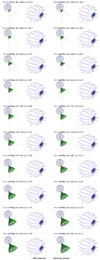 |
Fig. A.2. Same as Fig. A.1, but for June 8, 2024. |
| In the text | |
Current usage metrics show cumulative count of Article Views (full-text article views including HTML views, PDF and ePub downloads, according to the available data) and Abstracts Views on Vision4Press platform.
Data correspond to usage on the plateform after 2015. The current usage metrics is available 48-96 hours after online publication and is updated daily on week days.
Initial download of the metrics may take a while.