| Issue |
A&A
Volume 695, March 2025
|
|
|---|---|---|
| Article Number | A230 | |
| Number of page(s) | 21 | |
| Section | Numerical methods and codes | |
| DOI | https://doi.org/10.1051/0004-6361/202452180 | |
| Published online | 26 March 2025 | |
Euclid preparation
LXII. Simulations and non-linearities beyond Lambda cold dark matter. 1. Numerical methods and validation
1
Department of Astrophysics, University of Zurich,
Winterthurerstrasse 190,
8057
Zurich, Switzerland
2
Institute of Cosmology and Gravitation, University of Portsmouth,
Portsmouth
PO1 3FX, UK
3
Dipartimento di Fisica e Astronomia, Università di Bologna,
Via Gobetti 93/2,
40129
Bologna, Italy
4
INAF-Osservatorio di Astrofisica e Scienza dello Spazio di Bologna,
Via Piero Gobetti 93/3,
40129
Bologna, Italy
5
INFN-Sezione di Bologna,
Viale Berti Pichat 6/2,
40127
Bologna, Italy
6
Max Planck Institute for Gravitational Physics (Albert Einstein Institute),
Am Muhlenberg 1,
14476
Potsdam-Golm, Germany
7
Institute of Space Sciences (ICE, CSIC), Campus UAB, Carrer de Can Magrans, s/n,
08193 Barcelona,
Spain
8
Institut de Ciencies de l’Espai (IEEC-CSIC), Campus UAB, Carrer de Can Magrans, s/n Cerdanyola del Vallés,
08193 Barcelona,
Spain
9
Laboratoire Univers et Théorie, Observatoire de Paris, Université PSL, Université Paris Cité, CNRS,
92190 Meudon,
France
10
Institute of Theoretical Astrophysics, University of Oslo, PO Box 1029 Blindern,
0315 Oslo,
Norway
11
Jet Propulsion Laboratory, California Institute of Technology,
4800 Oak Grove Drive,
Pasadena,
CA
91109, USA
12
Max-Planck-Institut für Astrophysik,
Karl-Schwarzschild-Str. 1,
85748
Garching, Germany
13
Department of Physics, Institute for Computational Cosmology, Durham University, South Road,
DH1 3LE,
UK
14
Jodrell Bank Centre for Astrophysics, Department of Physics and Astronomy, University of Manchester, Oxford Road,
Manchester
M13 9PL, UK
15
INAF-IASF Milano,
Via Alfonso Corti 12,
20133
Milano, Italy
16
Istituto Nazionale di Fisica Nucleare, Sezione di Bologna,
Via Irnerio 46,
40126
Bologna, Italy
17
Institute for Astronomy, University of Edinburgh, Royal Observatory, Blackford Hill,
Edinburgh
EH9 3HJ, UK
18
Higgs Centre for Theoretical Physics, School of Physics and Astronomy, The University of Edinburgh,
Edinburgh
EH9 3FD, UK
19
Institut für Theoretische Physik, University of Heidelberg,
Philosophenweg 16,
69120
Heidelberg, Germany
20
Institut de Recherche en Astrophysique et Planétologie (IRAP), Université de Toulouse, CNRS, UPS, CNES, 14 Av. Edouard Belin,
31400 Toulouse,
France
21
Université St Joseph; Faculty of Sciences,
Beirut,
Lebanon
22
Institut de Physique Théorique, CEA, CNRS, Université Paris-Saclay
91191
Gif-sur-Yvette Cedex, France
23
School of Mathematics and Physics, University of Surrey, Guildford, Surrey,
GU2 7XH,
UK
24
INAF-Osservatorio Astronomico di Brera,
Via Brera 28,
20122
Milano, Italy
25
IFPU, Institute for Fundamental Physics of the Universe,
via Beirut 2,
34151
Trieste, Italy
26
INAF-Osservatorio Astronomico di Trieste,
Via G. B. Tiepolo 11,
34143
Trieste, Italy
27
INFN, Sezione di Trieste,
Via Valerio 2,
34127
Trieste TS, Italy
28
SISSA, International School for Advanced Studies,
Via Bonomea 265,
34136
Trieste TS, Italy
29
INAF-Osservatorio Astrofisico di Torino,
Via Osservatorio 20,
10025
Pino Torinese (TO), Italy
30
Dipartimento di Fisica, Università di Genova, Via Dodecaneso 33, 16146,
Genova,
Italy
31
INFN-Sezione di Genova,
Via Dodecaneso 33,
16146
Genova, Italy
32
Department of Physics “E. Pancini”, University Federico II, Via Cinthia 6, 80126,
Napoli,
Italy
33
INAF-Osservatorio Astronomico di Capodimonte,
Via Moiariello 16,
80131
Napoli, Italy
34
INFN section of Naples,
Via Cinthia 6,
80126
Napoli, Italy
35
Instituto de Astrofísica e Ciências do Espaço, Universidade do Porto, CAUP,
Rua das Estrelas,
4150-762
Porto, Portugal
36
Faculdade de Ciências da Universidade do Porto,
Rua do Campo de Alegre,
4150-007
Porto, Portugal
37
Aix-Marseille Université, CNRS, CNES, LAM,
Marseille,
France
38
Dipartimento di Fisica, Università degli Studi di Torino,
Via P. Giuria 1,
10125
Torino, Italy
39
INFN-Sezione di Torino,
Via P. Giuria 1,
10125
Torino, Italy
40
INAF – Osservatorio Astronomico di Roma,
Via Frascati 33,
00078
Monteporzio Catone, Italy
41
INFN-Sezione di Roma, Piazzale Aldo Moro 2, c/o Dipartimento di Fisica, Edificio G. Marconi,
00185 Roma,
Italy
42
Centro de Investigaciones Energéticas, Medioambientales y Tecnológicas (CIEMAT),
Avenida Complutense 40,
28040
Madrid, Spain
43
Port d’Informació Científica, Campus UAB,
C. Albareda s/n,
08193
Bellaterra (Barcelona), Spain
44
Institute for Theoretical Particle Physics and Cosmology (TTK), RWTH Aachen University,
52056 Aachen,
Germany
45
Institut d’Estudis Espacials de Catalunya (IEEC), Edifici RDIT, Campus UPC, 08860 Castelldefels,
Barcelona,
Spain
46
Dipartimento di Fisica e Astronomia “Augusto Righi” – Alma Mater Studiorum Università di Bologna,
Viale Berti Pichat 6/2,
40127
Bologna, Italy
47
Instituto de Astrofísica de Canarias, Calle Vía Láctea s/n, 38204, San Cristóbal de La Laguna,
Tenerife,
Spain
48
European Space Agency/ESRIN, Largo Galileo Galilei 1, 00044 Frascati,
Roma,
Italy
49
ESAC/ESA, Camino Bajo del Castillo, s/n., Urb. Villafranca del Castillo, 28692 Villanueva de la Cañada,
Madrid,
Spain
50
Université Claude Bernard Lyon 1, CNRS/IN2P3, IP2I Lyon, UMR 5822,
Villeurbanne
69100, France
51
Institute of Physics, Laboratory of Astrophysics, Ecole Polytechnique Fédérale de Lausanne (EPFL), Observatoire de Sauverny,
1290 Versoix,
Switzerland
52
Institut de Ciències del Cosmos (ICCUB), Universitat de Barcelona (IEEC-UB),
Martí i Franquès 1,
08028
Barcelona, Spain
53
Institució Catalana de Recerca i Estudis Avançats (ICREA),
Passeig de Lluís Companys 23,
08010
Barcelona, Spain
54
UCB Lyon 1, CNRS/IN2P3, IUF, IP2I Lyon, 4 rue Enrico Fermi,
69622 Villeurbanne,
France
55
Departamento de Física, Faculdade de Ciências, Universidade de Lisboa,
Edifício C8, Campo Grande,
1749-016
Lisboa, Portugal
56
Instituto de Astrofísica e Ciências do Espaço, Faculdade de Ciências, Universidade de Lisboa,
Campo Grande,
1749-016
Lisboa, Portugal
57
Department of Astronomy, University of Geneva,
ch. d’Ecogia 16,
1290
Versoix, Switzerland
58
Université Paris-Saclay, CNRS, Institut d’astrophysique spatiale,
91405 Orsay,
France
59
INFN – Padova,
Via Marzolo 8,
35131
Padova, Italy
60
INAF – Istituto di Astrofisica e Planetologia Spaziali, via del Fosso del Cavaliere,
100,
00100
Roma, Italy
61
Université Paris-Saclay, Université Paris Cité, CEA, CNRS, AIM,
91191,
Gif-sur-Yvette, France
62
FRACTAL S.L.N.E.,
calle Tulipán 2, Portal 13 1A,
28231,
Las Rozas de Madrid, Spain
63
INAF – Osservatorio Astronomico di Padova,
Via dell’Osservatorio 5,
35122
Padova, Italy
64
Max Planck Institute for Extraterrestrial Physics,
Giessenbachstr. 1,
85748
Garching, Germany
65
Universitäts-Sternwarte München, Fakultät für Physik, Ludwig-Maximilians-Universität München,
Scheinerstrasse 1,
81679
München, Germany
66
Dipartimento di Fisica “Aldo Pontremoli”, Università degli Studi di Milano,
Via Celoria 16,
20133
Milano, Italy
67
Felix Hormuth Engineering,
Goethestr. 17,
69181
Leimen, Germany
68
Technical University of Denmark,
Elektrovej 327,
2800
Kgs. Lyngby, Denmark
69
Cosmic Dawn Center (DAWN),
Denmark
70
Université Paris-Saclay, CNRS/IN2P3, IJCLab,
91405 Orsay,
France
71
Max-Planck-Institut für Astronomie,
Königstuhl 17,
69117
Heidelberg, Germany
72
NASA Goddard Space Flight Center,
Greenbelt,
MD
20771, USA
73
Department of Physics and Astronomy, University College London, Gower Street,
London
WC1E 6BT, UK
74
Department of Physics and Helsinki Institute of Physics,
Gustaf Hällströmin katu 2, 00014 University of Helsinki,
Finland
75
Aix-Marseille Université, CNRS/IN2P3, CPPM,
Marseille,
France
76
Université de Genève, Département de Physique Théorique and Centre for Astroparticle Physics,
24 quai Ernest-Ansermet,
1211
Genève 4, Switzerland
77
Department of Physics, PO Box 64,
00014 University of Helsinki,
Finland
78
Helsinki Institute of Physics, Gustaf Hällströmin katu 2, University of Helsinki,
Helsinki,
Finland
79
NOVA optical infrared instrumentation group at ASTRON, Oude Hoogeveensedijk 4,
7991PD Dwingeloo,
The Netherlands
80
Centre de Calcul de l’IN2P3/CNRS,
21 avenue Pierre de Coubertin
69627
Villeurbanne Cedex, France
81
Universität Bonn, Argelander-Institut für Astronomie,
Auf dem Hügel 71,
53121
Bonn, Germany
82
Dipartimento di Fisica e Astronomia “Augusto Righi” – Alma Mater Studiorum Università di Bologna,
via Piero Gobetti 93/2,
40129
Bologna, Italy
83
Université Paris Cité, CNRS, Astroparticule et Cosmologie,
75013 Paris,
France
84
University of Applied Sciences and Arts of Northwestern Switzerland, School of Engineering,
5210 Windisch,
Switzerland
85
Institut d’Astrophysique de Paris, 98bis Boulevard Arago,
75014 Paris,
France
86
Institut d’Astrophysique de Paris, UMR 7095, CNRS, and Sorbonne Université, 98 bis boulevard Arago,
75014 Paris,
France
87
Institut de Física d’Altes Energies (IFAE), The Barcelona Institute of Science and Technology,
Campus UAB,
08193
Bellaterra (Barcelona), Spain
88
European Space Agency/ESTEC,
Keplerlaan 1,
2201
AZ Noordwijk, The Netherlands
89
DARK, Niels Bohr Institute, University of Copenhagen,
Jagtvej 155,
2200
Copenhagen, Denmark
90
Waterloo Centre for Astrophysics, University of Waterloo, Waterloo,
Ontario
N2L 3G1, Canada
91
Department of Physics and Astronomy, University of Waterloo, Waterloo,
Ontario
N2L 3G1, Canada
92
Perimeter Institute for Theoretical Physics, Waterloo,
Ontario
N2L 2Y5, Canada
93
Space Science Data Center, Italian Space Agency, via del Politecnico snc,
00133 Roma,
Italy
94
Centre National d’Etudes Spatiales – Centre spatial de Toulouse,
18 avenue Edouard Belin,
31401
Toulouse Cedex 9, France
95
Institute of Space Science, Str. Atomistilor, nr. 409 Măgurele, Ilfov,
077125,
Romania
96
Dipartimento di Fisica e Astronomia “G. Galilei”, Università di Padova,
Via Marzolo 8,
35131
Padova, Italy
97
Departamento de Física, FCFM, Universidad de Chile, Blanco Encalada 2008,
Santiago,
Chile
98
Universität Innsbruck, Institut für Astro- und Teilchenphysik,
Technikerstr. 25/8,
6020
Innsbruck, Austria
99
Satlantis,
University Science Park, Sede Bld
48940,
Leioa-Bilbao, Spain
100
Instituto de Astrofísica e Ciências do Espaço, Faculdade de Ciências, Universidade de Lisboa,
Tapada da Ajuda,
1349-018
Lisboa, Portugal
101
Universidad Politécnica de Cartagena, Departamento de Electrónica y Tecnología de Computadoras,
Plaza del Hospital 1,
30202
Cartagena, Spain
102
Kapteyn Astronomical Institute, University of Groningen,
PO Box 800,
9700
AV Groningen, The Netherlands
103
INFN-Bologna,
Via Irnerio 46,
40126
Bologna, Italy
104
Dipartimento di Fisica, Università degli studi di Genova, and INFN-Sezione di Genova,
via Dodecaneso 33,
16146
Genova, Italy
105
Infrared Processing and Analysis Center, California Institute of Technology,
Pasadena,
CA
91125, USA
106
INAF, Istituto di Radioastronomia,
Via Piero Gobetti 101,
40129
Bologna, Italy
107
Astronomical Observatory of the Autonomous Region of the Aosta Valley (OAVdA),
Loc. Lignan 39,
11020,
Nus (Aosta Valley), Italy
108
Institute of Astronomy, University of Cambridge, Madingley Road,
Cambridge
CB3 0HA, UK
109
School of Physics and Astronomy, Cardiff University, The Parade,
Cardiff
CF24 3AA, UK
110
Junia, EPA department, 41 Bd Vauban,
59800 Lille,
France
111
ICSC – Centro Nazionale di Ricerca in High Performance Computing, Big Data e Quantum Computing, Via Magnanelli 2,
Bologna,
Italy
112
Instituto de Física Teórica UAM-CSIC, Campus de Cantoblanco,
28049 Madrid,
Spain
113
CERCA/ISO, Department of Physics, Case Western Reserve University,
10900 Euclid Avenue,
Cleveland,
OH
44106, USA
114
INFN-Sezione di Milano,
Via Celoria 16,
20133
Milano, Italy
115
Departamento de Física Fundamental. Universidad de Salamanca. Plaza de la Merced s/n,
37008 Salamanca,
Spain
116
Departamento de Astrofísica, Universidad de La Laguna, 38206 La Laguna,
Tenerife,
Spain
117
Dipartimento di Fisica e Scienze della Terra, Università degli Studi di Ferrara,
Via Giuseppe Saragat 1,
44122
Ferrara, Italy
118
Istituto Nazionale di Fisica Nucleare, Sezione di Ferrara,
Via Giuseppe Saragat 1,
44122
Ferrara, Italy
119
Center for Data-Driven Discovery, Kavli IPMU (WPI), UTIAS, The University of Tokyo,
Kashiwa, Chiba
277-8583,
Japan
120
Ludwig-Maximilians-University,
Schellingstrasse 4,
80799
Munich, Germany
121
Max-Planck-Institut für Physik,
Boltzmannstr. 8,
85748
Garching, Germany
122
Dipartimento di Fisica – Sezione di Astronomia, Università di Trieste,
Via Tiepolo 11,
34131
Trieste, Italy
123
Minnesota Institute for Astrophysics, University of Minnesota,
116 Church St SE,
Minneapolis,
MN
55455, USA
124
Institute Lorentz, Leiden University,
Niels Bohrweg 2,
2333
CA Leiden, The Netherlands
125
Université Côte d’Azur, Observatoire de la Côte d’Azur, CNRS, Laboratoire Lagrange,
Bd de l’Observatoire, CS 34229,
06304
Nice cedex 4, France
126
Institute for Astronomy, University of Hawaii,
2680 Woodlawn Drive,
Honolulu,
HI
96822, USA
127
Department of Physics & Astronomy, University of California Irvine,
Irvine
CA 92697, USA
128
Department of Astronomy & Physics and Institute for Computational Astrophysics, Saint Mary’s University,
923 Robie Street,
Halifax, Nova Scotia
B3H 3C3,
Canada
129
Departamento Física Aplicada, Universidad Politécnica de Cartagena, Campus Muralla del Mar, 30202 Cartagena,
Murcia,
Spain
130
Instituto de Astrofísica de Canarias (IAC); Departamento de Astrofísica, Universidad de La Laguna (ULL),
38200,
La Laguna,
Tenerife, Spain
131
Department of Physics, Oxford University, Keble Road,
Oxford
OX1 3RH, UK
132
CEA Saclay, DFR/IRFU, Service d’Astrophysique,
Bat. 709,
91191
Gif-sur-Yvette, France
133
Department of Computer Science, Aalto University,
PO Box 15400,
Espoo 00
076, Finland
134
Instituto de Astrofísica de Canarias, c/ Via Lactea s/n, La Laguna E-38200, Spain. Departamento de Astrofísica de la Universidad de La Laguna, Avda. Francisco Sanchez,
La
Laguna 38200, Spain
135
Ruhr University Bochum, Faculty of Physics and Astronomy, Astronomical Institute (AIRUB), German Centre for Cosmological Lensing (GCCL),
44780 Bochum,
Germany
136
Univ. Grenoble Alpes, CNRS, Grenoble INP, LPSC-IN2P3, 53, Avenue des Martyrs,
38000 Grenoble,
France
137
Department of Physics and Astronomy,
Vesilinnantie 5,
20014 University of Turku,
Finland
138
Serco for European Space Agency (ESA), Camino bajo del Castillo, s/n, Urbanizacion Villafranca del Castillo, Villanueva de la Cañada,
28692 Madrid,
Spain
139
ARC Centre of Excellence for Dark Matter Particle Physics,
Melbourne,
Australia
140
Centre for Astrophysics & Supercomputing, Swinburne University of Technology, Hawthorn,
Victoria
3122, Australia
141
School of Physics and Astronomy, Queen Mary University of London, Mile End Road,
London
E1 4NS, UK
142
Department of Physics and Astronomy, University of the Western Cape, Bellville,
Cape
Town 7535, South Africa
143
ICTP South American Institute for Fundamental Research, Instituto de Física Teórica, Universidade Estadual Paulista,
São Paulo, Brazil
144
IRFU, CEA, Université Paris-Saclay
91191
Gif-sur-Yvette Cedex, France
145
Oskar Klein Centre for Cosmoparticle Physics, Department of Physics, Stockholm University,
Stockholm
106 91, Sweden
146
Astrophysics Group, Blackett Laboratory, Imperial College London,
London
SW7 2AZ, UK
147
INAF-Osservatorio Astrofisico di Arcetri,
Largo E. Fermi 5,
50125
Firenze, Italy
148
Dipartimento di Fisica, Sapienza Università di Roma,
Piazzale Aldo Moro 2,
00185
Roma, Italy
149
Centro de Astrofísica da Universidade do Porto,
Rua das Estrelas,
4150-762
Porto, Portugal
150
Dipartimento di Fisica, Università di Roma Tor Vergata, Via della Ricerca Scientifica 1,
Roma,
Italy
151
INFN, Sezione di Roma 2, Via della Ricerca Scientifica 1,
Roma,
Italy
152
HE Space for European Space Agency (ESA), Camino bajo del Castillo, s/n, Urbanizacion Villafranca del Castillo, Villanueva de la Cañada,
28692 Madrid,
Spain
153
Aurora Technology for European Space Agency (ESA), Camino bajo del Castillo, s/n, Urbanizacion Villafranca del Castillo, Villanueva de la Cañada,
28692 Madrid,
Spain
154
INAF-Osservatorio Astronomico di Brera, Via Brera 28, 20122 Milano, Italy, and INFN-Sezione di Genova, Via Dodecaneso 33, 16146,
Genova,
Italy
155
Theoretical astrophysics, Department of Physics and Astronomy, Uppsala University,
Box 515,
751
20 Uppsala, Sweden
156
Department of Physics, Royal Holloway, University of London
TW20 0EX,
UK
157
Mullard Space Science Laboratory, University College London, Holmbury St Mary, Dorking,
Surrey
RH5 6NT, UK
158
Department of Astrophysical Sciences, Peyton Hall, Princeton University,
Princeton,
NJ
08544, USA
159
Niels Bohr Institute, University of Copenhagen,
Jagtvej 128,
2200
Copenhagen, Denmark
160
Center for Cosmology and Particle Physics, Department of Physics, New York University,
New York,
NY
10003, USA
161
Center for Computational Astrophysics, Flatiron Institute,
162 5th Avenue,
New York,
NY
10010, USA
★ Corresponding author; julian.adamek@uzh.ch
Received:
9
September
2024
Accepted:
5
December
2024
To constrain cosmological models beyond ACDM, the development of the Euclid analysis pipeline requires simulations that capture the non-linear phenomenology of such models. We present an overview of numerical methods and N-body simulation codes developed to study the non-linear regime of structure formation in alternative dark energy and modified gravity theories. We review a variety of numerical techniques and approximations employed in cosmological N-body simulations to model the complex phenomenology of scenarios beyond ACDM. This includes discussions on solving non-linear field equations, accounting for fifth forces, and implementing screening mechanisms. Furthermore, we conduct a code comparison exercise to assess the reliability and convergence of different simulation codes across a range of models. Our analysis demonstrates a high degree of agreement among the outputs of different simulation codes, typically within 2% for the predicted modification of the matter power spectrum and within 4% for the predicted modification of the halo mass function, although some approximations degrade accuracy a bit further. This provides confidence in current numerical methods of modelling cosmic structure formation beyond ACDM. We highlight recent advances made in simulating the non-linear scales of structure formation, which are essential for leveraging the full scientific potential of the forthcoming observational data from the Euclid mission.
Key words: methods: numerical / dark matter / dark energy / large-scale structure of Universe
© The Authors 2025
 Open Access article, published by EDP Sciences, under the terms of the Creative Commons Attribution License (https://creativecommons.org/licenses/by/4.0), which permits unrestricted use, distribution, and reproduction in any medium, provided the original work is properly cited.
This article is published in open access under the Subscribe to Open model. Subscribe to A&A to support open access publication.
1 Introduction
Significant progress in cosmological observations is expected in the upcoming years, in particular from the Euclid survey (Laureijs et al. 2011; Euclid Collaboration: Mellier et al. 2025; Euclid Collaboration: Scaramella et al. 2022; Nesseris et al. 2022; Martinelli et al. 2021; Euclid Collaboration: Castro et al. 2023), Vera Rubin Observatory’s Legacy Survey of Space and Time (LSST, Ivezić et al. 2019), the Roman Space Telescope (Spergel et al. 2015), and the Dark Energy Spectroscopic Instrument (DESI, DESI Collaboration: Aghamousa et al. 2016). These surveys will offer precision observations to high redshifts, allowing us to study the evolution of the Universe with unprecedented accuracy and potentially uncover the nature of dark matter and dark energy (DE). Gaining a deeper understanding of the nature of DE and addressing the long-standing question of whether the cosmological constant (A) is responsible for the late-time accelerated expansion of the Universe is indeed one of the primary goals of the Euclid survey (Amendola et al. 2018).
The Euclid space telescope was launched on July 1 2023 and is going to observe billions of galaxies out to redshift z ≈ 2, covering more than a third of the sky in optical and near-infrared wavelengths. Euclid will deliver precise measurements of the shapes and redshifts of galaxies (Euclid Collaboration: Bretonnière et al. 2022, 2023; Euclid Collaboration: Merlin et al. 2023; Euclid Collaboration: Desprez et al. 2020; Euclid Collaboration: Ilbert et al. 2021), from which we shall measure weak gravitational lensing (Euclid Collaboration: Ajani et al. 2023) and galaxy clustering (Euclid Collaboration: Adam et al. 2019). These primary probes can be used to rigorously investigate different cosmological scenarios, in particular those related to DE that go beyond the Lambda cold dark matter (ACDM) concordance model.
Although the ACDM model is generally very successful in matching observations, the true identities of CDM and the cosmological constant A remain unknown. Additionally, some tensions have persisted in recent years, most notably the Hubble tension (see Di Valentino et al. 2021a, for a summary and references) whereby local measurements of the Hubble parameter today, H0, appear to disagree with those inferred from high-redshift observations by around 5 σ. Further examples are the S8 tension (see Di Valentino et al. 2021b, for a summary and references) and some anomalies found in measurements of the cosmic microwave background (Abdalla et al. 2022). The presence of these tensions may hint at a breakdown of the ACDM model and further motivates the exploration of alternative scenarios.
Over the past few years, cosmologists have explored different possibilities to account for the late-time accelerating expansion of the Universe (Tsujikawa 2010; Clifton et al. 2012; Joyce et al. 2016) either by introducing a new field, referred to as the DE field, or by proposing a modified theory of gravity (MG). A wide range of MG or DE models is equivalent to adding a new light scalar degree of freedom to the theory of general relativity (GR).
In these theories, the scalar degree of freedom exhibits time evolution, sometimes accompanied by spatial fluctuations within the cosmic horizon. Even in the absence of such fluctuations, the background evolution may be different from ACDM, leading to modifications in structure formation. Significant spatial fluctuations in these models may arise due to various factors, including a low characteristic speed of sound in the theory (Gleyzes et al. 2014; Hassani et al. 2019), or as a result of the non-minimal coupling of the scalar field to matter or gravity (see Amendola 2004, for an example). The MG and DE theories featuring a coupling of the scalar field to matter can further affect perturbations at sub-horizon scales by mediating a fifth force. If the coupling is universal and includes baryons, a screening mechanism is essential to evade the precise constraints of local experiments (Will 2014). Screening mechanisms are typically achieved through non-linear phenomena in such theories. If, on the other hand, the coupling to matter is non-universal and confined entirely to the dark sector, local experiments have no constraining power, and cosmological observations provide the main constraints.
Given the diversity of possible DE or MG scenarios, a large information gain is expected from non-linear scales in the cosmological large-scale structure. These scales must be studied using N-body simulations that capture the essential aspects of the DE or MG models under consideration. This usually means that at least one additional equation needs to be solved for the extra degree of freedom. In many cases, this leads to a difficult non-linear problem that could require special techniques or approximations that need to be developed. This makes N -body simulations for models of DE or MG a challenging task.
In this paper, we first review the main features of the different classes of DE and MG models that have been proposed over the past years (see also Amendola et al. 2018, and Frusciante et al., in prep. for a more comprehensive and detailed overview). For each of them, we then discuss the numerical methods implemented within a selection of existing N-body codes (summarised in Table 1). Focussing on MG models with a universal coupling, we then compare the results of different N-body implementations for two well-studied theories; namely, the Hu–Sawicki f (R) gravity (Hu & Sawicki 2007) and the ‘normal branch’ of the Dvali–Gabadadze–Porrati braneworld model (nDGP, Dvali et al. 2000; Schmidt 2009a). We choose simulation parameters following the code comparison paper by Winther et al. (2015) [W15 hereafter], allowing us to validate a number of new codes against existing results.
This article is part of a series that collectively explores simulations and non-linearities beyond the ACDM model:
Numerical methods and validation (this work).
Results from non-standard simulations (Euclid Collaboration: Rácz et al. 2025).
Constraints on f(R) models from the photometric primary probes (Euclid Collaboration: Koyama et al. 2024).
Cosmological constraints on non-standard cosmologies from simulated Euclid probes (D’Amico et al., in prep.).
The purpose of this first article in the series is to serve as a reference for models beyond ACDM and their existing implementations in various codes. This paper is structured as follows. In Sect. 2, we give a broad overview of different numerical approaches to treating the additional physics of models beyond ACDM. In Sect. 3, we discuss a number of different codes that implement those approaches and carry out a validation exercise, comparing several recently developed codes with the existing state-of-the-art ones. We conclude in Sect. 4. In an appendix, we discuss some performance considerations.
Summary table of the N-body codes implementing various extensions to the standard ACDM cosmology that have been used to produce simulations employed in Euclid pre-launch analysis, validation, and forecasting.
2 Methods
2.1 Non-standard background evolution
A wide range of models beyond the simplest cosmological constant scenario are based on an additional scalar degree of freedom – for example, a classical scalar field, ϕ – that evolves dynamically in the expanding Universe and whose background energy density, ρϕ, provides the source for the observed DE abundance. To induce cosmic acceleration and to match existing constraints on the background expansion history, the equation-of-state parameter, w, of such an additional field must be sufficiently negative at recent epochs but is poorly constrained at earlier times. This allows for models where w also evolves dynamically as long as it converges to values close to w ≈ −1 in the late Universe. For these models, the DE component modifies the background expansion history of the Universe, which is encoded by the general expression of the Hubble function,

where ΩX denotes the density parameter of constituent X = m, r, k, DE for matter, radiation, curvature and DE, respectively, and the equation-of-state parameter, w, of DE can be obtained by solving the background field equations – including the evolution of the additional scalar degree of freedom ϕ – or can be parameterised. A common parameterisation suggested by Chevallier, Polarski & Linder (CPL, Chevallier & Polarski 2001; Linder 2003) is based on the desired evolution of w at low redshifts,

Alternatively, one can set the desired relative abundance of DE at late (ΩDE = 1 − Ωm) and early (ΩEDE) epochs as in the early dark energy (EDE, Wetterich 2004) parameterisation,

The modified expansion history expressed by Eq. (1) will indirectly affect the evolution of matter density fluctuations and modify the formation process of collapsed structures by changing the Hubble friction term in the equation for linear matter perturbations, which in Newtonian gauge and in Fourier space for sub-horizon scales reads:

where δm and δDE are the density contrasts of matter and DE perturbations, respectively, G is Newton’s constant, and a dot represents a derivative with respect to cosmic time.
Besides the richer background dynamics that is endowed by an evolving field, whenever DE is promoted from a cosmological constant to a dynamical degree of freedom, the model also acquires an additional layer of complexity: the presence and evolution of DE fluctuations around the mean-field configuration. This corresponds to the situation where δDE in Eq. (4) is non-negligible, whereas in ACDM it would vanish identically at all scales. Like any other density perturbations, inhomogeneities in the DE would then contribute to the peculiar gravitational potential that governs the evolution of matter perturbations and thus the formation of cosmic structures, as is shown by Eq. (4).
However, in many of the simplest scalar-field scenarios, such perturbations are negligible at sub-horizon scales because the speed of sound, cs, of the scalar field is naturally close to the speed of light. Ignoring them for the purpose of numerical simulations, the only modification of N-body algorithms required to simulate these DE models is given by an appropriate calculation of the cosmic expansion rate. The most common approach amounts to tabulating the specific expansion rate of the universe for the model to be simulated according to Eq. (1) and replacing the standard analytical calculation of the Hubble function within the N-body algorithm with an interpolated value from the tabulated solution that is provided to the code as an input. This approach is implemented by most of the simulation codes employed within the Euclid Collaboration to perform cosmological simulations in homogeneous DE models beyond ACDM.
2.2 Linearised dark energy perturbations
Although a wide range of DE models are characterised by negligible DE fluctuations, as was discussed above, some specific scenarios may not fulfil this condition at all scales and/or at all times (Kodama & Sasaki 1984; Amendola 2004). This can occur either because they feature a lower value of the DE speed of sound – the speed at which perturbations in the DE field propagate – allowing DE perturbations to grow on scales above the associated Jeans length that then falls inside the cosmological horizon, or because additional interactions – besides gravity – can induce the growth of such perturbations. The former case corresponds to the class of clustering DE models, while the latter is known as coupled DE.
2.2.1 Clustering dark energy
The clustering DE models are characterised by two time-dependent variables: the speed of sound, cs, and the equation of state parameter, w. In these theories, the DE component clusters on scales larger than the associated sound horizon or Jeans scale, λs = H/cs, and DE perturbations decay quickly below the sound-horizon scale. For a sufficiently small speed of sound, we may even expect non-linear DE structures to form. At a fundamental level, clustering DE models are analogous to the k-essence type of theories, so that the action reads (Armendariz-Picon et al. 2001)
![$S = \int {{{\rm{d}}^4}} x\sqrt { - g} \left[ {\frac{{{c^4}R}}{{16\pi G}} + P(X,\phi ) + {{\cal L}_{\rm{m}}}} \right],$](/articles/aa/full_html/2025/03/aa52180-24/aa52180-24-eq5.png)
where P is a general function of the kinetic term  and the scalar field ϕ, and ℒm is the matter Lagrangian. For a given P(X, ϕ), the speed of sound and the equation of state are given by (Armendariz-Picon et al. 2000)

where the subscript ‘, X’ denotes the partial derivative with respect to X. We therefore need to specify the function P(X, ϕ) to derive the equations of motion for the k-essence scalar field. However, since there are many possible choices, we can instead employ the effective field theory of DE (EFT) approach to model the dynamics of k-essence DE. The EFT framework, although not a fundamental theory, offers several advantages (Gleyzes et al. 2014; Cheung et al. 2008), such as being a description of a wide range of theories within some scales. The EFT is a perturbative approach based on the assumption that the scalar field perturbations remain small over the scales of interest. It is worth noting that the regime of non-linear matter clustering is accessible to the EFT framework as long as the scalar field perturbations remain small (Hassani et al. 2019). While the EFT framework is useful for describing DE theories in a minimal way at relevant cosmological scales, it is inherently limited to small scalar field perturbations (low-energy limits) of an underlying theory, assuming that higher-energy interactions are suppressed. Additionally, the EFT framework is often constructed without a clear connection to a fundamental theory, making it challenging to translate constraints on EFT parameters into meaningful constraints on a fundamental theory.
The k-essence theories or clustering DE models are implemented in several N-body and Einstein–Boltzmann codes. In CLASS (Lesgourgues 2011) and CAMB (Lewis et al. 2000), these theories are implemented using the fluid picture. In hi_class (Zumalacárregui et al. 2017), the EFT equations are implemented and can be controlled using the EFT parameter  within the code. On the other hand, in k-evolution (Hassani et al. 2019, 2020), which is an N-body code based on gevolution (Adamek et al. 2016a), non-linear equations for clustering DE are implemented as an independent component, and the k-essence field for small cs can form non-linear structures. In some N-body codes, for example in gevolution (Adamek et al. 2016b), clustering DE is implemented through a linear solution from an Einstein–Boltzmann solver. This is a good assumption for large speeds of sound, but for small ones, this method does not allow for the response of DE to the non-linear matter structures.
2.2.2 Coupled quintessence
Moving to the case of coupled DE models, the interaction can be formulated at a fundamental level by introducing a direct coupling between the scalar field and the spatial curvature R in the so-called Jordan frame (see e.g. Pettorino & Baccigalupi 2008), so that the action reads
![$S = \int {{{\rm{d}}^4}} x\sqrt { - g} \left[ {\frac{{{c^4}f(\phi ,R)}}{{16\pi G}} - \frac{1}{2}Z(\phi ){\nabla ^\mu }\phi {\nabla _\mu }\phi - V(\phi ) + {{\cal L}_{\rm{m}}}} \right],$](/articles/aa/full_html/2025/03/aa52180-24/aa52180-24-eq9.png)
where f(ϕ, R) is a function that couples the scalar field to the curvature, Z(ϕ) is a function that allows for non-standard kinetic terms, V(ϕ) is the scalar field self-interaction potential, and the matter Lagrangian contains at least one cold species characterised by some rest mass, m0.
Alternatively, the interaction can be formulated by including source terms in the covariant conservation equations of the interacting species in the so-called Einstein frame1,


![${\nabla ^\mu }T_{\mu \nu }^{(\phi )} = \frac{1}{{{M_{{\rm{Pl}}}}}}\left[ {{\beta _{({\rm{c}})}}(\phi ){T^{({\rm{c}})}} + {\beta _{({\rm{b}})}}(\phi ){T^{({\rm{b}})}}} \right]{\nabla _\nu }\phi ,$](/articles/aa/full_html/2025/03/aa52180-24/aa52180-24-eq12.png)
where  is the stress-energy tensor of a given species Y, T(Y) is its trace, β(Y)(ϕ) is the coupling function of species Y, the labels c, b, ϕ refer to the dark matter, baryon, and scalar field species, respectively, and MP1 ≡ (ℏc)1/2(8πG)−1/2 is the reduced Planck mass.
While in the former case the interaction will necessarily be universal (i.e. involving all matter species with the same strength, as the field ϕ couples directly with the scalar curvature R), which goes under the name of extended quintessence, the latter approach allows for non-universal couplings that may selectively involve individual species, for example by separately choosing the coupling functions for baryons and dark matter.
In the case of a universal coupling (that is, if β(b) = β(c)), the two approaches can be related to one another through a Weyl transformation of the metric (see again Pettorino & Baccigalupi 2008), and are therefore equivalent. On the other hand, the possibility to leave the baryonic component of the Universe only minimally coupled evades Solar System constraints (see e.g. Will 2014) on the deviations from standard gravity thereby avoiding the need for screening mechanisms. This is the case of Coupled Quintessence models (Wetterich 1995; Amendola 2000), where the direct coupling between the scalar field and massive (non-baryonic) particles can support stable perturbations of the DE field at sub-horizon scales (see e.g. Amendola 2004). In general, such perturbations may even become non-linear in the presence of a sufficiently strong coupling (as in the case of Growing Neutrino Quintessence models, see e.g. Amendola et al. 2008; Mota et al. 2008; Baldi 2012b; Ayaita et al. 2016). Nonetheless, a large class of widely studied coupled DE models is known to feature scalar perturbations of the order of the standard Newtonian gravitational potential (δϕ ~ ΦN, see again Amendola 2004, for an extended derivation), thereby remaining in the linear regime at all times and scales of cosmological interest. This allows us to linearise the corresponding field equations and derive modified equations of motions for massive particles, including the contribution of the additional force arising from the direct coupling with the scalar field (see e.g. Baldi 2011).
In fact, a general feature of coupled DE models is the existence of a ‘fifth force’ mediated by the scalar field. The new force can be expressed as an additional acceleration experienced by a massive coupled particle, which in comoving coordinates will be given by

where Y identifies a coupled matter species, and δϕ is the scalar field fluctuation. This extra acceleration term is added to the standard Newtonian acceleration acting on all massive particles,

where u is the peculiar particle velocity in comoving coordinates, and ΦN is the peculiar Newtonian potential obeying the standard Poisson equation

where the sum runs over all clustering species in the Universe.
Therefore, solving for the dynamical evolution of massive coupled particles requires solving for the scalar field perturbation δϕ entering in Eq. (11), which in the most general case follows a non-linear elliptic equation,

with F a function of the scalar field fluctuation δϕ, and where the sum runs over all the coupled matter species with their respective couplings β(Y)(ϕ).
For the particular case of a coupled DE model with a nonuniversal interaction (Damour et al. 1990) involving only dark matter and leaving baryons uncoupled (i.e. β(b) = 0) the function F(δϕ) in Eq. (14) is negligible compared to the term associated with matter density perturbations (see Amendola 2004, for a derivation) and can be safely discarded. As a result, the scalar-field equation reduces to

where Φc is the Newtonian potential generated by the distribution of the coupled dark matter particles, which is

Therefore, the solution for the scalar field perturbations will be directly proportional to the potential, Φc, according to the relation

The acceleration equation for a coupled particle can then be rewritten as

assuming here for simplicity that other clustering species (such as massive neutrinos) give a negligible contribution to the total Newtonian potential such that ΦN = Φc + Φb. This modified acceleration equation introduces a further modification to be implemented in N-body simulation codes for Coupled Quintessence cosmologies besides the specific expansion history of each particular model. This often requires substantial modifications in the gravity solvers of conventional N-body codes, as the algorithms need to evolve coupled and uncoupled massive particles (typically dark matter and baryons, respectively) with different equations and should therefore treat these components separately. Even under the approximation of a purely collisionless treatment (i.e. ignoring the hydrodynamical and astrophysical processes that affect standard baryonic matter leading to the formation of stars and galaxies) that is often employed for large-volume simulations targeted at galaxy surveys such as Euclid, both coupled and uncoupled matter species must be included in the simulation to provide a consistent representation of the dynamics at all scales: as baryons and dark matter evolve differently, assuming that all matter is dark would lead to an overestimation of the effects of the coupling and, thus, biased results. This approach is implemented in the C-Gadget code (Baldi et al. 2010; Baldi 2012a) that is employed for coupled DE simulations performed within the Euclid Collaboration. Thanks to this feature, the C-Gadget code may allow one to run simulations of Coupled DE models that also include more sophisticated treatments of galaxy formation processes that may affect the observational properties of galaxies (Fontanot et al. 2015) or other observables related to the intergalactic medium (see e.g. Baldi & Viel 2010).
Distinguishing between coupled and uncoupled particle types in simulations of coupled quintessence is also crucial for proper treatment of two other effects that characterise these cosmological models beyond the fifth force described by Eq. (11). The first is the mass variation of coupled particles due to the exchange of rest-frame energy with the DE scalar field, which arises as a direct consequence of the modified continuity equations (8) and of the assumption of particle number conservation. More specifically, the mass of coupled particles evolves as a result of the evolution of the background scalar field according to

Such a mass variation, which involves only particle species with a non-vanishing coupling to the scalar field, must be taken into account in N-body algorithms by changing the mass of individual simulation particles at every time step. This is normally done by tabulating the mass as a function of scale factor a by numerically integrating Eq. (19) along with the background dynamics of the scalar field ϕ, and interpolating from that table as the simulation progresses.
The second effect is an additional force (on top of the fifth force) acting on coupled particles as a consequence of momentum conservation due to the particles’ mass variation described by Eq. (19), which takes the form of a velocity-dependent extra acceleration behaving either as a friction or as a drag, depending on the relative signs of the coupling function β(ϕ) and of the scalar field velocity ϕ (see e.g. Baldi et al. 2010),

Such a velocity-dependent acceleration is responsible for a very rich phenomenology characterising Coupled Quintessence models, especially on highly non-linear scales (see e.g. Baldi et al. 2010; Baldi 2012a, 2023; Li & Barrow 2011), and must be included in N-body simulations as well for a fully consistent treatment of these scenarios. This is done by adding the extra acceleration described in Eq. (20) to the total acceleration (i.e. Newtonian plus fifth force) of all coupled particles in each time step,

The relevant quantities β(ϕ) and ϕ can again be interpolated from a table obtained by integrating the background dynamics of the system. This is the approach implemented in the C-Gadget code that has been used to run Coupled Quintessence simulations within the Euclid Collaboration.
2.2.3 Momentum exchange and dark scattering
A further example of interacting DE cosmologies characterised by scalar-field perturbations that always remain linear is given by models of pure momentum exchange (see e.g. Pourtsidou et al. 2013; Skordis et al. 2015) between the DE field and massive particles like dark matter or baryons. A limiting case is given by the dark scattering scenario (Simpson 2010) where the momentum transfer between the two components is modelled as the elastic scattering of massive particles moving through a homogeneous DE fluid with equation of state w. This results in an extra force acting on the moving massive particles that is proportional to their comoving velocity, similar to the velocity-dependent force described by Eq. (20) for Coupled Quintessence models. However, the origin of this force is completely different in this case, as it does not originate from the mass variation of particles but rather from the momentum transfer with the DE field. As a result, the scattering acceleration can be expressed as

where the parameter ξ is defined as

with σ denoting the scattering cross section and m the typical mass of the scattering particle species.
This type of interaction can be implemented in N-body algorithms (see e.g. Baldi & Simpson 2015, 2017) in a very similar way as the velocity-dependent acceleration in Coupled Quintessence scenarios, as the factors entering Eq. (22) are all either constants or background quantities that can be interpolated at every timestep from tabulated data. This is the approach implemented in the C–Gadget code that has been used to run the DAKAR and DAKAR2 simulations (Baldi & Simpson 2017; Euclid Collaboration: Rácz et al. 2025).
Although dark scattering represents a limiting case of the more general class of pure momentum-exchange models between matter and DE (also known as ‘Type 3’ models in the classification of Skordis et al. 2015), for which further modifications to the standard particle dynamics are expected besides the drag force of Eq. (22), recent works (Palma & Candlish 2023) have shown that such additional modifications are generally subleading with respect to the drag force so that their effect on structure formation can be neglected. This ensures that the current implementation of dark scattering within the simulations used in the Euclid Collaboration can be considered representative of the general class of momentum-exchange cosmologies.
2.3 Non-linear scalar field perturbations
In models where a scalar field couples to matter universally, or at least to baryons in a relevant way, some mechanism to suppress the coupling is required to satisfy the stringent local tests of gravity. This is commonly referred to as ‘screening’. Screening mechanisms are achieved by non-linearity in the scalar-field equation coupled to matter. The equation determining the evolution of the scalar field is typically a wave equation of the form

Here, □ = ∇µ∇µ represents the d’Alembertian operator and S is a non-linear function that depends on the matter density, the scalar field, and its derivatives. Various methods have been developed to solve this non-linear scalar field equation in N-body simulations, where the non-linear density ρm is modelled by collisionless particles (see W15, for more details).
Several approximations are often used to solve these nonlinear equations. The most common one is the quasi-static approximation. The scalar field can be split into a background part,  , and a perturbation, δϕ, as
  . The quasi-static approximation amounts to ignoring the time dependence of the scalar field perturbation; that is, assuming
  . The partial differential equation (PDE) of the field perturbation, which in its original form may have been of the hyperbolic or parabolic type, is therefore cast into an elliptic form so that the scalar field solution at any given time depends solely on the matter configuration at that time. This is a good approximation whenever the speed of sound of the scalar field is small (Sawicki & Bellini 2015), which is the case for the MG models considered here. Non-quasistatic cosmological simulations have been conducted for several MG models using different techniques, such as the explicit leap-frog method and the implicit Newton–Gauss–Seidel method (Llinares & Mota 2013; Bose et al. 2015; Winther & Ferreira 2015b).
The scalar-field solution is required for the computation of the total gravitational potential, Φ, that acts on the matter particles,

where the effective density depends on the scalar field. There are two common ways of solving for this total gravitational force. The first option is to solve first for ϕ and then use this solution to compute the source term in Eq. (25) and solve for Φ using a standard Poisson solver to get the total force ∇Φ. The other option is to apply the total force ∇ΦN + ∇ϕ to the particles.
Under the quasi-static approximation, the scalar-field equation assumes the same form as the usual Poisson equation,

The main difference is that the scalar-field equation is generally non-linear. This non-linear behaviour implies that conventional techniques, such as using Fourier analysis, cannot be used to solve the equation. Numerous approaches have been developed to address this challenge, and we refer the reader to W15 for details. For computational methods that aim to accurately solve a non-linear equation on refined grids, the approach typically involves discretising the equation in a suitable way and employing an iterative algorithm, such as the Newton–Raphson method, to successively refine solutions based on an initial guess. To speed up convergence, many of these methods incorporate so-called ‘multigrid’ acceleration techniques that we quickly review here.
2.3.1 Non-linear multigrid algorithm
A generic way to solve non-linear elliptic PDEs is to couple the multigrid algorithm to the Newton–Raphson method,

where u is the discretised field, ℒ is the differential operator (which is a Laplacian for Newtonian gravity) and the superscripts refer to the new or old estimate of the solution in one Newton–Raphson iteration. The Newton–Raphson method produces linear equations for the correction terms, which are solved by the full-approximation storage multigrid algorithm (Brandt 1977; Wesseling 2004; Guillet & Teyssier 2011). For a review of these methods applied to MG simulations, see e.g. Li (2018), Llinares (2018) and W15.
A simple sketch of the algorithm goes as follows. One starts with a guess for the solution on a grid; this could be anything from a constant value across the grid to using the solution from the previous timestep in the simulation. One then loops a few times over all cells in the grid, updating the solution using Eq. (27). This solution is then restricted to a grid with half the resolution, the solution is updated again, and this process is repeated recursively up to the coarsest grid (one with only 23 cells). The solution is then interpolated to the finer grid, updated once more, and this is done recursively until one reaches the finest grid we started with. One such cycle is called a V-cycle, and one repeats such V-cycles until convergence is achieved. The advantage of having this stack of coarser grids is that it helps to accelerate the convergence of the largest modes in the solution.
2.3.2 Screening with non-linearity in potentials
In models where screening is achieved by non-linearity in a potential or coupling function, the equation for the scalar field becomes

where β(ϕ) and V(ϕ) are non-linear functions of ϕ. A typical example is f(R) gravity. In this class of models, the value of the scalar field changes by orders of magnitude. To enhance numerical stability, a common technique involves redefining the scalar field in terms of a new variable. The redefinition to choose depends on the specific model under consideration. It is typically chosen to prevent the occurrence of unphysical values of the scalar field during Newton–Raphson iterations. For example, for f(R) models the scalar field ϕ = f,R will be driven towards zero in high-density regions, but at the same time f,R cannot cross zero, as the potential becomes singular in this scenario. To avoid this issue, a commonly used field redefinition is ![$u \equiv \ln \left[ {{f_{,R}}/{{\bar f}_{,R}}(a)} \right]$](/articles/aa/full_html/2025/03/aa52180-24/aa52180-24-eq35.png) (Oyaizu 2008). However, this transformation introduces additional non-linearity and in some models, such as Hu–Sawicki f(R) models, this transformation is not necessary and might even lead to considerable performance losses in a simulation.
(Oyaizu 2008). However, this transformation introduces additional non-linearity and in some models, such as Hu–Sawicki f(R) models, this transformation is not necessary and might even lead to considerable performance losses in a simulation.
In some cases, this can be avoided. For example, Bose et al. (2017) noticed that for Hu–Sawicki f(R) gravity with n = 1 (Hu & Sawicki 2007), when making the change of variable  , the field equation could be recast as a depressed cubic equation,

which possesses analytical solutions (Ruan et al. 2022). Although the Gauss-Seidel smoothing procedure is still needed (because p depends on the values of the field u in neighbouring cells), this removes the Newton–Raphson part and expensive exponential/logarithmic operations from the method of Oyaizu (2008), therefore leading to significant performance gains. Ruan et al. (2022) also generalised this improved relaxation approach to the cases of n = 0 (which strictly speaking is not a variation of the Hu–Sawicki model) and n = 2.
For other models like the symmetron, which has a Higgs-like potential, the scalar field is free to cross zero, and no field redefinition is needed (apart from a simple re-scaling).
2.3.3 Screening with non-linearity in kinetic terms
In another class of models, non-linearity emerges within the kinetic term. For example, in models with the Vainshtein screening mechanism (Vainshtein 1972), the equation exhibits non-linearity in the second derivatives of the scalar field,

where β(a) is a time-dependent coupling function. The simplest example here is the DGP model (Dvali et al. 2000), which was first simulated by Schmidt (2009b). In such cases, the operator-splitting trick (Chan & Scoccimarro 2009) can be employed. This approach can simplify the equations, avoiding potential issues associated with imaginary square roots, and improving code performance. This trick is particularly useful for the DGP braneworld models and other Vainshtein screening models, such as Cubic and Quartic Galileons (see Sect. 4.2.2 of W15, for more information).
2.3.4 Approximate treatments of screening
Some models allow linearisation of the non-linear equation using some approximation. One approach (Khoury & Wyman 2009; Winther & Ferreira 2015a; see also the appendix of Schmidt 2009a) is to introduce the screening factor for the matter density perturbation

where the screening function depends on the Newtonian potential Φn. This type of parameterised modified gravity is referred to as ‘type 1’ in Table 1. One specific method, developed in Brando et al. (2023), starts from linearising Klein–Gordon’s equation. In this formalism, one solves the Poisson equation in Fourier space,

where the function Geff(a, k) approximates the effective Newton’s constant introduced by the screening effect of the scalar field on small scales. This function is given by

with  being the asymptotic linear effective Newton’s constant that depends only on time, and M(a, k) is a function that approximately captures the non-linear corrections introduced by the scalar field on small scales. This function allows Eq. (33) to transition from
  on large scales to Geff(a, k) → G on small scales. This type of parameterised modified gravity is referred to as ‘type 2’ in Table 1. A procedure to fix M(a, k) is described in Brando et al. (2023), which has the advantage of avoiding additional parameters to tune the screening efficiency.
One can also choose to parameterise the non-linear contribution using an effective Newton’s constant at both small and large scales. If the modifications of gravity are encoded in a scale-dependent function ΔGeff(a, k) as in Eq. (33), then we can propose a similar equation in real space,

where  is the Fourier transform of ΔGeff(a, k). In practice, an additional approximation is made, namely ΔGeff(a, r) ≈ ΔGeff (a, k → 1/r).
This approach allows for the encoding of non-linear contributions over the whole range of scales modelled by N-body algorithms through real-space equations, for instance, the Tree Particle-Mesh (TreePM) method implemented in codes like Gadget 4. Provided the parameterisation is effective, this is expected to increase the accuracy of the estimation of the non-linear effects.
Several parameterisations have been proposed for this kind of approach, either with additional tuning parameters, such as in Lombriser (2016), or based on local small-scale environmental properties to avoid the need for any extra parameters, such as in Winther & Ferreira (2015a).
3 Additional code validation
A code comparison for simulations that solve non-linear scalar field perturbations is presented in W15. Since then, various new codes have been developed. In this section, we show a comparison of the predictions for the power spectrum and the halo mass function using the simulations of W15 as a reference and starting from the same initial conditions. These were generated using second-order Lagrangian perturbation theory in a ACDM cosmology with Ωm = 0.269, ΩA = 0.731, h = 0.704, ns = 0.966 and σ8 = 0.801. The simulations have Np = 5123 particles of mass Mp ≃ 8.756 × 10⁹ h−1 M⊙ in a box of side length L = 250 h−1 Mpc and start at redshift z = 49. Box size and mass resolution are chosen to cover the transition from quasi-linear to non-linear scales. In particular, for the f(R) gravity model considered here, the Compton wavelength,  , associated with the scalar degree of freedom, f,R, takes the value λC ≈ O(10) h−1 Mpc at the present epoch. As in W15, we compare simulations for f(R) and nDGP models. In these models (Schmidt 2009a), the background expansion history is closely approximated by that of ACDM. Furthermore, the effect of modified gravity can be ignored at z = 49, thus it is justified to use the initial conditions of ACDM. The measurements of the power spectrum and mass function are performed by the pipeline developed in the second article of this series, Euclid Collaboration: Rácz et al. (2025). Based on two models only, our comparison does not encompass the full diversity of numerical methods discussed in the previous section. In many cases some validation of the various implementations can be found in the corresponding references.
3.1 Summary of codes used in the validation
Table 1 shows an overview of the simulation codes considered in this section and provides a quick reference of their capabilities and limitations. For each of them, a short summary is presented here. In the Appendix we comment on the trade-off between accuracy and computational cost of the implementations. The parameter files and initial data of the simulations used in this section are curated on a public repository2.
3.1.1 MG–Arepo
First presented in Arnold et al. (2019), this code is based on the moving-mesh N-body and hydrodynamical simulation code Arepo (Springel 2010; Weinberger et al. 2020), which uses a TreePM algorithm to calculate gravitational forces. The additional modified gravity force (fifth force) is calculated with a relaxation solver (Bose et al. 2017) that is accelerated by the multigrid method and uses adaptive mesh refinement (AMR). It currently also supports simulations for the nDGP model (Hernández-Aguayo et al. 2021), as well as massive neutrinos implemented using the δf method (Elbers et al. 2021).
To solve the modified gravity equations, the density field is projected onto the AMR grid, constructed in such a way that each cell on the highest refinement level contains at most one particle (except if a pre-set maximum refinement level is reached; the cell size at this level is of the order of the smoothing length of the standard gravity solver). Once the field equation is solved to obtain the scalar field configuration, the modified gravity force can be computed from its gradient using finite differencing.
Since MG–Arepo computes the forces on all particles simultaneously, and the modified gravity field equations are generally highly non-linear (with a poor convergence rate of the relaxation algorithm), this is computationally expensive compared to Arepo’s Newtonian gravity solver. However, the maximum acceleration of the modified gravity force is smaller than that of Newtonian gravity, mainly because the latter occurs in regions with high density where screening occurs. This allows the modified gravity solver to run using larger time steps (Arnold et al. 2019), resulting in significantly reduced computational cost. Together with Arepo’s efficient MPI parallelisation and lean memory footprint, these have made it possible to run the large number of f(R) simulations used in various recent works, such as the FORGE-BRIDGE (Arnold et al. 2022; Harnois-Déraps et al. 2023; Ruan et al. 2024) simulation suite of 200 f(R) and nDGP models. This has allowed accurate emulators of various physical quantities or observables to be constructed.
Another highlight of MG–Arepo is its capability to run realistic galaxy formation simulations in a cosmological box (Arnold et al. 2019; Hernández-Aguayo et al. 2021), thanks to the use of the Illustris-TNG subgrid physics model (Weinberger et al. 2017; Pillepich et al. 2018). More recently, it has been used for larger-box hydrodynamical simulations with a realistic recalibrated Illustris-TNG model (Mitchell et al. 2022), enabling the study of galaxy clusters in modified gravity.
The MG-Arepo simulations used in this paper were run using a residual criterion of ϵ = 10−2 and a maximum refinement level (MaxAMRLevel) of 10 for the nDGP simulations and 18 for the f(R) models with a gravitational softening of 0.01 h−1 Mpc.
3.1.2 MG–Gadget
MG–Gadget (Puchwein et al. 2013) is a modified version of the TreePM N-body code Gadget–3 (which in turn is based on the public code Gadget–2, see Springel 2005) implementing an AMR solver for the scalar degree of freedom f,R characterising the widely studied Hu–Sawicki f(R) gravity model. In MG–Gadget, the same tree structure that is employed to solve for standard Newtonian gravity is also used as an adaptive grid to solve for the scalar field configuration through an iterative Newton–Gauss–Seidel (NGS) relaxation scheme (see Sect. 2.3) with the ‘full-approximation storage multigrid’ method (see Sect. 2.3.1) and with the field redefinition ![$u \equiv \ln \left[ {{f_{,R}}/{{\bar f}_{,R}}(a)} \right]$](/articles/aa/full_html/2025/03/aa52180-24/aa52180-24-eq47.png) (see Sect. 2.3.2). MG–Gadget also allows MG simulations to be run with massive neutrinos (see e.g. Baldi et al. 2014; Giocoli et al. 2018) using the neutrino particle method (see Adamek et al. 2023, for a review on numerical methods for massive neutrino simulations).
(see Sect. 2.3.2). MG–Gadget also allows MG simulations to be run with massive neutrinos (see e.g. Baldi et al. 2014; Giocoli et al. 2018) using the neutrino particle method (see Adamek et al. 2023, for a review on numerical methods for massive neutrino simulations).
For the simulations presented here, the relative tree opening criterion was used with an acceleration relative error threshold of 0.0025, and a uniform grid with 5123 cells was employed to compute long-range Newtonian forces. Concerning the MG field solver, a residual tolerance of ϵ = 10−2 was set for the V-cycle iteration and a maximum refinement level of 18 was used for the AMR grid, corresponding to a spatial resolution of 1 h−1 kpc at the finest grid level, compared to a gravitational softening of 18 h−1 kpc, following the setup adopted in W15.
3.1.3 ECOSMOG
ECOSMOG (Li et al. 2012) is a generic modified gravity simulation code based on the publicly available N-body and hydrody-namical simulation code RAMSES (Teyssier 2002). Originally developed for f(R) gravity, this code takes advantage of the adaptive mesh refinement of RAMSES to achieve the high resolution needed to solve the scalar field and hence the fifth force in high-density regions. The non-linear f(R) field equation is solved with the standard Gauss-Seidel approach as first applied by Oyaizu (2008), but it was later replaced by the more efficient algorithm of Bose et al. (2017). The code has since been extended for simulations for the generalised chameleon (Brax et al. 2013), symmetron and dilaton (Brax et al. 2012), nDGP (Li et al. 2013b), cubic Galileon (Barreira et al. 2013, 2015), quartic Galileon (Li et al. 2013a), vector Galileon (Becker et al. 2020) and nonlocal gravity (Barreira et al. 2014).
For the ECOSMOG simulations used in this paper, we have used a domain grid (the uniform mesh that covers the whole simulation domain) with 29 = 512 cells per dimension, and the cells are hierarchically refined if they contain 8 or more effective3 particles. The highest refined levels have effectively 216 cells, leading to a force resolution of about 0.0075 h−1 Mpc.
3.1.4 ISIS
The ISIS code (Llinares et al. 2014), like the ECOSMOG code above, is based on RAMSES (Teyssier 2002). It contains a scalar field solver that can be used to simulate generic MG models with non-linear equation of motion and has been used to simulate models such as f(R) gravity, the symmetron model, nDGP and disformal coupled models (Gronke et al. 2014; Winther & Ferreira 2015a; Winther et al. 2015; Hagala et al. 2016; Llinares et al. 2020). It also allows for hydrodynamical simulations that have been used to study the interplay between baryonic physics and modified gravity (Hammami et al. 2015). Furthermore, the code has the capability to go beyond the quasistatic limit and study the full time dependence of the scalar field (Llinares & Mota 2013; Llinares & Mota 2014; Hagala et al. 2017). The scalar field solver used in the code is a Gauss–Seidel relaxation method with multigrid acceleration, very similar to the one in ECOSMOG described above.
For the ISIS simulations presented in this paper, we have used a domain grid (the uniform mesh that covers the whole simulation domain) with 29 = 512 cells per dimension, and the cells are hierarchically refined if they contain 8 or more effective particles.
3.1.5 PySCo
PySCo4 (Breton 2025) is a particle-mesh (PM) code written in Python and accelerated with Numba that currently supports Newtonian and f(R) gravity (parameterised as in Hu & Sawicki 2007, with n = 1 or n = 2). While multiple flavours of solvers based on Fast Fourier Transforms (FFT) are available, for the present paper, we use a multigrid solver to propose something different from other codes in this comparison project (other codes that also use multigrid are AMR-based). PySCo uses a triangular-shaped cloud mass assignment scheme and solves the linear Poisson equation using multigrid V-cycles with a tolerance threshold of the residual of 10−3, and two F-cycles (such cycles go through the mesh levels more often than V-cycles, resulting in a higher convergence rate of the residuals at the cost of increased runtime. For details on multigrid cycles see also Ruan et al. 2022) to solve the additional field in f(R) gravity with the non-linear multigrid method described in Sect. 2.3.1 and Eq. (29). Our convergence threshold is very conservative since we do not intend to conduct a convergence study in this paper (a less conservative threshold could still give reasonable results at much lower computational cost). Furthermore, to resolve the small scales we use a coarse grid with 20483 cells, resulting in roughly 500 time steps to complete the simulations.
3.1.6 MG–COLA
MG–COLA simulations were performed using the Fourier-Multigrid Library FML5. These simulations are based on the COmoving Lagrangian Acceleration (COLA) method (Tassev et al. 2013), which combines Lagrangian perturbation theory with the PM method to reduce the number of time steps that are required to recover clustering on large scales. The MG–COLA N-body solver in the FML library contains implementations of various DE and MG models like the DGP model, the symmetron model, f(R) gravity and the Jordan–Brans–Dicke model (see Winther et al. 2017, for more details). For the PM part, we used  ; that is, a mesh discretisation five times smaller than the mean particle separation, and the total of 150 time-steps linearly spaced along the scale factor to achieve a good agreement of the mass function with AMR simulations. We also ran low-resolution simulations with
  with 100 time steps, and checked that the non-linear enhancement of the power spectrum from these low-resolution simulations agrees well with the one from the high-resolution ones. Screening is included using approximate treatments described in Sect. 2.3.4. For f(R) gravity models, the FML code has one parameter to tune the strength of chameleon screening called screening efficiency. For the model with
  , we used the default value screening efficiency = 1 while we used screening efficiency =2 for
  , and the parameter
  refers to
  evaluated at redshift z = 0. Setting screening efficiency = 1 implies that we use the screening condition obtained by the spherical approximation (Winther & Ferreira 2015a). Fiorini et al. (2021) introduced a screening efficiency, fs, to increase or decrease the screening strength. This is an empirical factor that needs to be calibrated by comparing with simulations that solve the scalar field equation exactly, and the choices used in this work were calibrated on the baseline simulations from MG–Arepo. Furthermore, this factor will depend on simulation parameters such as the mass and force resolutions as well as the number of time steps. A more sophisticated procedure to calibrate this factor was proposed in Saadeh et al. (2024). For nDGP, we used Gaussian smoothing with a smoothing radius of 1 h−1 Mpc to compute the density field for screening and did not use an option to enforce the linear solution at small wavenumbers k. We also ran simulations based on the screening approximation using Geff(a, k) given by Eq. (33) for nDGP, and in these simulations, we have used the same COLA settings as in the other screening approximation implementation. The biggest advantage of this screening implementation is that it does not require any additional tuning parameter related to screening; that is, the function Geff(a, k) is completely defined by the theoretical model one wants to simulate.
3.1.7 PANDA
PANDA is an extension of the TreePM code Gadget4. It introduces modifications at large scales in the PM part with an effective Newton’s constant according to Eq. (33), while the force at small scales is modified in the tree part with Eq. (34). In this respect, PANDA implements an approximate solver for the extra force induced by different possible MG theories. On the other hand, differently from other approximate methods, the dynamics of matter particles under the effect of the (dominant) standard gravity force is treated with the full TreePM solver of Gadget4 of which it retains the accuracy in modelling the non-linear density field. For nDGP, the functional form of  is described in Lombriser (2016), while for f (R) it is introduced as in Winther & Ferreira (2015a). In the latter case, no additional parameters are needed to describe the screening. For the first nDGP case instead, in addition to the theoretically defined parameters N0 = 1, B = 1/[3β(a)], b = 2 and a = 3, we consider the screening scale kth = 0.4 h Mpc−1 defined by the parameterisation

where rV is the Vainshtein radius of the model for a spherically symmetric density perturbation (see Lombriser 2016, for more details).
3.2 Comparison of the power spectrum
Before discussing the effect of extra degrees of freedom, we compare the different codes within a ACDM cosmology. For reference and only for the case of ACDM, we include results from the code PKDGRAV3 that was also used for the Flagship simulations in Euclid (Potter et al. 2017; Euclid Collaboration: Castander et al. 2025). Figure 1 shows the matter power spectra at two different redshifts, z = 1 (left panels) and z = 0.667 (right panels). The lower panels show the relative difference to the simulation carried out with MG-Arepo that we use as a reference throughout. Since ISIS and ECOSMOG have both been developed from the RAMSES code, the agreement between these two codes is better than 1%. These AMR codes tend to underestimate the power on small scales when compared to tree-based codes, mainly due to the mesh refinement criterion used in our simulations. Fine-tuning some precision parameters, we expect that a better agreement can be achieved, cf. Schneider et al. (2016). As we can see, the codes that perform closely to our benchmark at small scales are the ones that also share the same tree-PM gravity solver, PANDA and MG–Gadget. PKDGRAV3, which uses a tree structure and the fast multipole method to compute gravitational forces, is in excellent agreement with MG–Gadget up to k ~ 1 h Mpc−1, yielding slightly more power at higher k.
Also shown in the figure are the results from COLA, a pure PM code that uses a fixed grid to solve the Poisson equation. The fixed resolution of the PM grid explains why COLA consistently suffers from low force resolution at k ≳ 1 h Mpc−1. All our simulations use the exact same initial particle data, such that our comparisons should not be contaminated by cosmic variance. However, for COLA simulations, we also reconstructed the initial density field from the initial particle distribution to estimate the displacement fields required for the 2LPT calculations in those simulations. While PySCo incorporates a full N-body solver, its small-scale accuracy is constrained by resolution limitations that arise from the absence of AMR. Moreover, within the scope of this code comparison project, PySCo employs a multigrid algorithm, resulting in reduced small-scale clustering compared to FFT (on a regular grid), thereby explaining the observed deficiency in power at wavenumbers k ≳ 1 h Mpc−1.
For modified gravity models, we compare the ratio between the power spectrum computed for that model and the one found in the ACDM reference cosmology. Taking such ratios largely cancels out the differences seen in ACDM between the codes, making the differences due to the treatments of the extra scalar field more apparent. Following W15, we consider two MG models that exhibit two different types of growth dependence and screening mechanisms. The first one is the so-called Hu-Sawicki f(R), which exhibits a scale-dependent growth factor at linear order, and a screening mechanism realised by non-linearities in the potential (see Sect. 2.3.2). The strength of the modification of gravity is characterised by the background value of the scalar degree of freedom, and we study the cases  and
and  , labelled ‘F5’ and ‘F6’, respectively, the latter being closer to GR. The second one is nDGP, a braneworld theory defined in a five-dimensional spacetime. The growth factor in this theory is scale independent, and screening is realised through non-linearities in the kinetic terms, as was discussed in Sect. 2.3.3. Here, the strength of the modification of gravity is characterised by the value of the cross-over scale, and we study the cases
  and
and  , labelled ‘N1.2’ and ‘N5.6’, respectively, the latter being closer to GR.
Figure 2 shows the relative change (with respect to ACDM) of the matter power spectrum due to modifications of gravity, sometimes called ‘boost’, for the two f(R) scenarios at red-shifts z = 1 (left panels) and z = 0.667 (right panels). Since f(R) already exhibits a scale-dependent growth factor at linear order, we can see that on scales of k ≈ 0.1 h Mpc−1 this effect is already present, and gets enhanced at large wavenumbers due to non-linearities of the density field. As we can see the codes MG–Arepo, MG–Gadget, ECOSMOG, ISIS, and PySCo all roughly agree to better than one percent down to scales of k ≈ 10 h Mpc−1, as was expected. These minor discrepancies can be caused by the refinement criterion used in the latter code or by slight variations in the redshift of the particle snapshot output. The present results are largely in agreement with a similar analysis performed in W15.
In the same plots, we can also see how approximation schemes to introduce screening from non-linearities in the potential perform in contrast to the exact solutions. The results that use these methods are showcased by the examples of COLA and PANDA, where each uses a different scheme to approximate the effects of the dynamics of the scalar field in dense environments. As was expected, the two codes do not exhibit the same level of agreement down to scales of k ≈ 10 h Mpc−1 as their counterparts using full solvers. However, in both cases, we can see that the deviations from the MG–Arepo reference results are limited to 2% even in the most extreme regime of departure from GR. Through closer inspection, we can see small differences in the agreement between the approximate schemes and full solvers at different values of k. These deviations are caused by different implementations of the approximate MG solvers in the two codes. In fact, while COLA is an approximate method that uses a PM algorithm to solve the Poisson equation on a fixed grid with the use of the screening approximation to linearise the Poisson equation, PANDA is a new implementation that exploits the TreePM structure of the baseline Gadget-4 code to solve for the small-scale particle dynamics by incorporating the MG effects (including the screening) through a scale-dependent Newton’s constant in both real and Fourier space.
Figure 3 shows results for the matter power spectra in the two nDGP scenarios we consider, characterised by the two values of the cross-over scale,  and
and  (N5.6). As before, we compare simulation results at two different redshifts, z = 1 (left panels) and z = 0.667 (right panels). Since the linear growth function has a scale-independent enhancement compared to ACDM, we see a constant amplification of power at small values of k. The Vainshtein mechanism suppresses the deviation from ACDM on small scales, leading to a diminishing boost at large k. The agreement between different codes at k < 1 h Mpc−1 is better than 1% for all codes, including the approximate simulations with COLA and PANDA. At k > 1 h Mpc−1, the AMR-based codes, ECOSMOG and ISIS, show larger deviations at the level of 2%, where the suppression of the deviation from ACDM is slightly underestimated compared with MG–Arepo. This could be caused by the difference in the ACDM power spectrum shown in Fig. 1, even though this difference in the baseline code is largely cancelled out in the boost. On the other hand, despite their approximations in the MG solvers, COLA and PANDA agree with MG–Arepo at the level of 1% even on these scales.
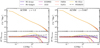 |
Fig. 1 Matter power spectra from simulations carried out with different codes (different line styles) for a ACDM cosmology. The left panels show the spectra at redshift z = 1 whereas the right panels show the spectra at redshift z = 0.667. The bottom panels show the relative difference with respect to the simulation carried out with MG–Arepo, see text for a discussion. The Nyquist wavenumber of the particle initial data is kNy ≈ 6.4 h Mpc−1. |
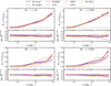 |
Fig. 2 Amplification factor of the matter power spectra from simulations of two f (R) scenarios, |


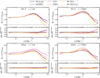 |
Fig. 3 Amplification factor of the matter power spectra from simulations of two nDGP scenarios, |


3.3 Comparison of the halo mass function
To gain further insight into the non-linear dynamics of the different models and their respective implementations we also compare the cumulative halo mass functions measured in our simulations. The impact of MG models on the structural properties of collapsed halos and on their mass distribution has been extensively investigated in the past by means of N-body simulations carried out with many of the codes considered in our comparison. Relevant results can be found in Cataneo et al. (2016) for ECOSMOG, Achitouv et al. (2016); Hagstotz et al. (2019) for MG–Gadget, Arnold & Li (2019) for MG–Arepo, and Fiorini et al. (2021) for MG–COLA. For the purpose of our comparison, halo catalogues are obtained with the Rockstar halo finder by running a pipeline described in the second paper of this series (Euclid Collaboration: Rácz et al. 2025). To establish the baseline for the comparison, in the spirit of the previous section, Fig. 4 shows a comparison of the cumulative halo mass function for the different codes in a ACDM cosmology. Since MG–Arepo and MG–Gadget are based on the same TreePM gravity solver, their agreement is excellent. They also agree very well with results from PKDGRAV3 that, as we like to remind the reader, are only available for the case of ACDM and are shown for reference here. On the other hand, ECOSMOG and ISIS are based on the AMR method. They agree with each other, but these simulations underestimate the abundance of low-mass halos below 1013h−1 M⊙. COLA uses a fixed-grid PM method, thus it also underestimates the abundance of low-mass halos. As was shown previously in Fiorini et al. (2021), COLA may underestimate the mass function at the low-mass end when the ROCKSTAR halo finder is used, mostly due to resolution effects. However, in this work, we find that with a relatively high resolution  , COLA agrees well with ECOSMOG and ISIS. We note that PySCo exhibits a similar behaviour to COLA, ECOSMOG and ISIS, albeit with a lower amplitude. This discrepancy can be attributed to the fact that PySCo has the least small-scale clustering (see Fig. 1), resulting in a smaller number of halos within the simulation.
The chameleon screening in f(R) depends on the halo mass such that high-mass halos are typically screened. The critical mass above which screening is effective is determined by the parameter  . As we can see from Fig. 5, the ratio of the halo mass function between f(R) and ACDM is enhanced for low-mass halos but approaches unity at the high-mass end where all halos are effectively screened. The agreement between full simulations (ECOSMOG and ISIS, MG–Arepo, MG–Gadget) is around 4% for all halo masses. Both COLA and PANDA employ an approximation for screening based on the thin-shell condition for a spherically symmetric object. Although this captures an overall effect of screening, it fails for low-mass halos in F6 and high-mass halos in F5, leading to larger deviations, which are found to be very similar for both codes.
In the case of the Vainshtein mechanism, there is no halo-mass dependence on the screening. Despite screening being effective inside dark matter halos, these halos still feel enhanced gravitational attraction. This increases the merger rate and ultimately leads to larger enhancements of the halo mass function for halos of larger masses. In nDGP, shown in Fig. 6, all codes agree within 4%, with a sub-per cent agreement seen in the intermediate mass range 1012 h−1 M⊙ < M < 1013 h−1 M⊙. The MG–COLA results with and without Geff(a, k) show slightly different levels of agreement. This is expected as the screening approximation with Geff (a, k) realises screening in Fourier space, whereas the one without is performed directly in real space. It is also worth noting that the screening approximation with Geff(a, k) was designed to implement screening in a fast way at the level of the matter power spectrum and other n-point statistics in Fourier space, and there is no guarantee that this works for the halo mass function. Nevertheless, both approaches are shown to agree well with each other. ECOSMOG shows a large deviation for M ≲ 5 × 10¹¹ h−1 M⊙. For these masses, there are fewer than 50 dark matter particles assigned to each halo, which indicates that the results could be affected by the refinement criteria of the simulations. The deviations are larger for the most massive halos, but the number of these halos is low and the halo mass function therefore becomes very noisy in this regime.
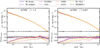 |
Fig. 4 Cumulative halo mass function from simulations carried out with different codes (different line styles) for a ACDM cosmology. The left panels show the halo mass function at redshift z = 1 whereas the right panels show the halo mass function at redshift z = 0.667. The bottom panels show the relative difference with respect to the simulation carried out with MG–Arepo. |
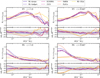 |
Fig. 5 Increase in the cumulative halo mass function from simulations for the two f(R) scenarios, |


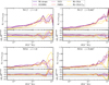 |
Fig. 6 Increase in the cumulative halo mass function from simulations for the two nDGP scenarios, |


4 Conclusions
In this work, we have presented a comprehensive review of numerical methods for cosmological N-body simulations in scenarios extending beyond the standard ACDM model. Our exploration spanned a variety of alternative DE and MG theories, highlighting the critical role of N-body simulations in connecting theoretical models with observational data. Through the detailed examination of numerical solvers and approximations tailored to these extended theories, we have showcased the state of the art of modelling the non-linear scales of cosmic structure formation under a wide range of cosmological scenarios. Our code comparison exercise, based on the simulations from W15 and extended by incorporating new codes and approximation techniques, has demonstrated a fair consensus among different numerical implementations. This validation is particularly important for the Euclid mission, as the forthcoming observational data will require precise non-linear modelling to constrain cosmological parameters effectively.
This article is part of a series that explores simulations and non-linearities in models beyond ACDM. The simulation codes that we have considered in this article are used to generate simulation products in the companion paper, Euclid Collaboration: Rácz et al. (2025), and are crucial for generating the simulations needed to create the non-linear modelling in the companion paper, Euclid Collaboration: Koyama et al. (2024), which forecasts constraints for f(R) gravity from photometric primary probes of the Euclid mission. The validation checks performed in this paper are therefore critical for being able to trust these results.
The main outcomes of this work can be summarised as follows:
N-body simulation codes have been developed for a wide range of extended cosmological scenarios, ranging from simple DE models to more complex interacting scalar field models and MG theories, to non-standard dark matter and initial conditions; the availability of such codes will be a crucial asset for the future developments of large galaxy surveys such as Euclid; we have provided a concise yet comprehensive overview of several such codes, their main features, implementation methods, assumptions and approximations;
As a matter of fact, among these simulation codes the ones involving algorithms for the solution of non-linear differential equations of some additional degrees of freedom, as e.g. for the case of MG theories, are the most challenging in terms of implementation and numerical convergence; we have therefore performed a thorough validation effort of these methods through a code comparison study, extending the approach adopted in W15 to more recent and diverse algorithms;
As a result of our validation effort, we found agreement in the power spectrum boost at ≲1% up to k ≲ 1 h Mpc−1 and at ≲3% up to k ≲ 10 h Mpc−1 among all the codes implementing full field solvers (MG-Arepo, MG-Gadget, ECOSMOG, ISIS, PySCo), while approximate methods (PANDA, MG-COLA) display slightly larger deviations not exceeding 3% up to k ≲ 7 h Mpc−1;
The halo mass function shows larger deviations among the codes, also due to larger differences in the outcomes for the baseline ACDM simulations; nonetheless, all codes agree within less than 5% on the relative change of the halo mass function except for the very largest and the smallest mass ranges where poor statistics and insufficient resolution, respectively, may impact the results;
We also compared the computational requirements of the different codes by measuring the CPU time needed to complete a reference MG simulation starting from identical initial conditions; we found that while full field solvers generally imply a substantial increase – up to a factor of ten – of the total CPU time relative to a ACDM simulation, approximate solvers are not significantly more demanding for MG simulations compared to standard ACDM runs.
Looking forwards, the continued evolution of simulation techniques will be paramount in leveraging the full potential of upcoming large-scale structure surveys such as Euclid. N-body simulations therefore continue to set a solid foundation for the next generation of cosmological inquiries. By persistently pushing the boundaries of computational astrophysics, we are poised to uncover the underlying physics driving the accelerated expansion of the Universe, thereby opening new windows onto the fundamental nature of DE, dark matter, and gravity itself.
Acknowledgements
We thank R.E. Smith for his diligent work as internal referee and P. Schneider for carefully proofreading the manuscript. The work of JA is supported by the Swiss National Science Foundation. During part of this work, AMCLB was supported by a fellowship of PSL University hosted by the Paris Observatory. This project was provided with computer and storage resources by GENCI at CINES thanks to the grant 2023-A0150402287 on the supercomputer Adastra’s GENOA partition. GR’s research was supported by an appointment to the NASA Postdoctoral Program administered by Oak Ridge Associated Universities under contract with NASA. GR was supported by JPL, which is run under contract by the California Institute of Technology for NASA (80NM0018D0004). The Euclid Consortium acknowledges the European Space Agency and a number of agencies and institutes that have supported the development of Euclid, in particular the Agenzia Spaziale Italiana, the Austrian Forschungsförderungsgesellschaft, funded through BMK, the Belgian Science Policy, the Canadian Euclid Consortium, the Deutsches Zentrum für Luft- und Raumfahrt, the DTU Space and the Niels Bohr Institute in Denmark, the French Centre National d’Etudes Spatiales, the Fundação para a Ciência e a Tecnologia, the Hungarian Academy of Sciences, the Ministerio de Ciencia, Innovatión y Universidades, the National Aeronautics and Space Administration, the National Astronomical Observatory of Japan, the Netherlandse Onderzoekschool Voor Astronomie, the Norwegian Space Agency, the Research Council of Finland, the Romanian Space Agency, the State Secretariat for Education, Research, and Innovation (SERI) at the Swiss Space Office (SSO), and the United Kingdom Space Agency. A complete and detailed list is available on the Euclid web site (http://www.euclid-ec.org).
Appendix A Computational cost
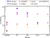 |
Fig. A.1 Comparison of the computational costs of simulations run under different gravity models (labels on the x-axis) and with different codes (markers and colours described in the legend). |
One of the obstacles in producing accurate predictions in the non-linear regime of structure formation is presented by the computational cost of running large N-body simulations. This issue becomes even more pronounced in the case of MG simulations, due to the additional computational cost associated with the solution of the Klein–Gordon equation for the scalar field describing the additional degree of freedom in these theories. To provide some insights into the trade-offs between accuracy and time-to-solution, we attempt here a comparative analysis of the computational cost of the simulations run for this paper. Given that these simulations were run on different machines and with different parallelisation settings, we cannot conduct a precise assessment of their computational cost. Instead, we limit this analysis to an order-of-magnitude comparison of the simulations run with the various codes and models discussed in this paper.
For this exercise, we use the information on the wall-clock time, Treal, and the number of cores, Ncores, recorded in the log files of the simulation runs. This information was available for all simulations except for the ones run with ISIS. We estimate the computational cost of the simulations, C, as the product of the wall-clock time and the number of cores:

The estimates of the computational cost for the simulations are compared in Fig. A.1. We can see that the cost of ACDM simulations of Tree-PM and AMR codes is C ~ 103 CPU hours, while for MG-COLA and PySCo the cost is about one order of magnitude lower at C ~ 102 CPU hours. For f (R) gravity models instead, the computational cost increases significantly (approximately by a factor of ten) for the codes that solve the full Klein–Gordon equation of the scalar field, namely MG-Arepo, MG-Gadget, ECOSMOG, and PySCo, while the overhead is smaller for the codes that adopt screening approximations, namely PANDA and MG–COLA. Finally, in nDGP gravity, only ECOSMOG has a significant overhead compared to ACDM, while MG-Arepo and the approximate codes, PANDA and MG-COLA, have just a small overhead.
The performance of multigrid codes depends on the convergence criterion chosen. For PySCo, we chose an extremely conservative approach (see Sect. 3.1.5) with a very low tolerance threshold, resulting in more V-cycles and almost double the CPU time needed to solve the linear Poisson equation compared to a more standard setup. Regarding the non-linear solver, we use two F-cycles instead of a single one (which should in principle be enough, but it is not the goal of the present paper to provide a convergence study), therefore roughly doubling the CPU time needed for the f(R) gravity models.
We stress that a thorough assessment of the efficiency of the codes is beyond the scope of this paper and would have required a much more methodical effort including (but not limited to)
running the simulations in a controlled environment,
conducting convergence tests for the various hyperparameters,
testing the scaling performance of each code.
In fact, when focussing only on predictions of the amplification factors, it is possible to achieve a similar level of accuracy with lower force, mass or time resolution, since resolution effects mostly cancel out when taking ratios of quantities affected by the same inaccuracies (Brando et al. 2022). This has been shown to be the case for MG–COLA simulations in Fiorini et al. (2023), where the use of a lower resolution allowed accurate predictions of power spectrum boosts in nDGP gravity with a theoretical gain of ~ 300 with respect to the computational cost of the COLA simulations presented here.
Such large speed-ups have paved the way for creating emulators for the non-linear amplification of the power spectrum in models beyond ACDM in a cost-effective way; that is, without the need for supercomputers. This has already been done for some of the models we consider in this paper (see e.g. Ramachandra et al. 2021; Mauland et al. 2024; Fiorini et al. 2023). For instance, Fiorini et al. (2023) found that an emulator for the nDGP model can be constructed with as little as a few thousand CPU hours worth of computational time. Likewise, Mauland et al. (2024) who presented a generic pipeline for using COLA to create such emulators, used f(R) gravity as an example and found similar numbers for the required computational time. Gordon et al. (2024) described a simulation setup that can also be used for emulating the full power spectrum (up to a reasonable high wavenumber k ~ 1 h Mpc−1), requiring around ~ 100 CPU hours per simulation on a modern CPU. Emulators have also been constructed for beyond-ACDM models using high-resolution direct simulations in the same way as has been done for ACDM. This approach generally gives more accurate emulators than those created with approximate methods, but this comes at a much higher cost. For example, both Sáez-Casares et al. (2024) and Arnold et al. (2022) have each presented a high-fidelity emulator for the f(R) model considered in this paper, but at a higher cost of about 3.5-4 million CPU hours.
References
- Abdalla, E., Abellán, G. F., Aboubrahim, A., et al. 2022, J. High Energy Astrophys., 34, 49 [NASA ADS] [CrossRef] [Google Scholar]
- Achitouv, I., Baldi, M., Puchwein, E., & Weller, J. 2016, Phys. Rev. D, 93, 103522 [NASA ADS] [CrossRef] [Google Scholar]
- Adamek, J., Daverio, D., Durrer, R., & Kunz, M. 2016a, Nature Phys., 12, 346 [Google Scholar]
- Adamek, J., Daverio, D., Durrer, R., & Kunz, M. 2016b, JCAP, 07, 053 [CrossRef] [Google Scholar]
- Adamek, J., Angulo, R. E., Arnold, C., et al. 2023, JCAP, 06, 035 [NASA ADS] [Google Scholar]
- Amendola, L. 2000, Phys. Rev. D, 62, 043511 [NASA ADS] [CrossRef] [Google Scholar]
- Amendola, L. 2004, Phys. Rev. D, 69, 103524 [Google Scholar]
- Amendola, L., Baldi, M., & Wetterich, C. 2008, Phys. Rev. D, 78, 023015 [NASA ADS] [Google Scholar]
- Amendola, L., Appleby, S., Avgoustidis, A., et al. 2018, Living Rev. Rel., 21, 2 [NASA ADS] [CrossRef] [Google Scholar]
- Armendariz-Picon, C., Mukhanov, V., & Steinhardt, P. J. 2000, Phys. Rev. Lett., 85, 4438 [Google Scholar]
- Armendariz-Picon, C., Mukhanov, V., & Steinhardt, P. J. 2001, Phys. Rev. D, 63, 103510 [NASA ADS] [CrossRef] [Google Scholar]
- Arnold, C., & Li, B. 2019, MNRAS, 490, 2507 [NASA ADS] [CrossRef] [Google Scholar]
- Arnold, C., Leo, M., & Li, B. 2019, Nature Astron., 3, 945 [Google Scholar]
- Arnold, C., Li, B., Giblin, B., Harnois-Déraps, J., & Cai, Y.-C. 2022, MNRAS, 515, 4161 [CrossRef] [Google Scholar]
- Ayaita, Y., Baldi, M., Führer, F., Puchwein, E., & Wetterich, C. 2016, Phys. Rev. D, 93, 063511 [Google Scholar]
- Baldi, M. 2011, MNRAS, 411, 1077 [NASA ADS] [CrossRef] [Google Scholar]
- Baldi, M. 2012a, MNRAS, 422, 1028 [NASA ADS] [CrossRef] [Google Scholar]
- Baldi, M. 2012b, ASP Conf. Ser., 453, 155 [NASA ADS] [Google Scholar]
- Baldi, M. 2023, MNRAS, 521, 613 [NASA ADS] [Google Scholar]
- Baldi, M., & Simpson, F. 2015, MNRAS, 449, 2239 [NASA ADS] [CrossRef] [Google Scholar]
- Baldi, M., & Simpson, F. 2017, MNRAS, 465, 653 [CrossRef] [Google Scholar]
- Baldi, M., & Viel, M. 2010, MNRAS, 409, 89 [Google Scholar]
- Baldi, M., Pettorino, V., Robbers, G., & Springel, V. 2010, MNRAS, 403, 1684 [CrossRef] [Google Scholar]
- Baldi, M., Villaescusa-Navarro, F., Viel, M., et al. 2014, MNRAS, 440, 75 [NASA ADS] [CrossRef] [Google Scholar]
- Barreira, A., Li, B., Hellwing, W. A., Baugh, C. M., & Pascoli, S. 2013, JCAP, 10, 027 [CrossRef] [Google Scholar]
- Barreira, A., Li, B., Hellwing, W. A., Baugh, C. M., & Pascoli, S. 2014, JCAP, 09, 031 [CrossRef] [Google Scholar]
- Barreira, A., Bose, S., & Li, B. 2015, JCAP, 12, 059 [CrossRef] [Google Scholar]
- Becker, C., Arnold, C., Li, B., & Heisenberg, L. 2020, JCAP, 10, 055 [CrossRef] [Google Scholar]
- Bose, S., Hellwing, W. A., & Li, B. 2015, JCAP, 02, 034 [CrossRef] [Google Scholar]
- Bose, S., Li, B., Barreira, A., et al. 2017, JCAP, 02, 050 [Google Scholar]
- Brando, G., Fiorini, B., Koyama, K., & Winther, H. A. 2022, JCAP, 09, 051 [NASA ADS] [Google Scholar]
- Brando, G., Koyama, K., & Winther, H. A. 2023, JCAP, 06, 045 [NASA ADS] [Google Scholar]
- Brandt, A. 1977, Math. Computat., 31, 333 [Google Scholar]
- Brax, P., Davis, A.-C., Li, B., Winther, H. A., & Zhao, G.-B. 2012, JCAP, 10, 002 [CrossRef] [Google Scholar]
- Brax, P., Davis, A.-C., Li, B., Winther, H. A., & Zhao, G.-B. 2013, JCAP, 04, 029 [CrossRef] [Google Scholar]
- Breton, M.-A. 2025, A&A, 695, A170 [NASA ADS] [CrossRef] [EDP Sciences] [Google Scholar]
- Cataneo, M., Rapetti, D., Lombriser, L., & Li, B. 2016, JCAP, 12, 024 [CrossRef] [Google Scholar]
- Chan, K. C., & Scoccimarro, R. 2009, Phys. Rev. D, 80, 104005 [NASA ADS] [Google Scholar]
- Cheung, C., Fitzpatrick, A. L., Kaplan, J., Senatore, L., & Creminelli, P. 2008, JHEP, 3, 014 [Google Scholar]
- Chevallier, M., & Polarski, D. 2001, Int. J. Mod. Phys. D, 10, 213 [Google Scholar]
- Clifton, T., Ferreira, P. G., Padilla, A., & Skordis, C. 2012, Phys. Rep., 513, 1 [NASA ADS] [CrossRef] [Google Scholar]
- Damour, T., Gibbons, G. W., & Gundlach, C. 1990, Phys. Rev. Lett., 64, 123 [Google Scholar]
- Deruelle, N., & Sasaki, M. 2011, Springer Proc. Phys., 137, 247 [NASA ADS] [Google Scholar]
- DESI Collaboration (Aghamousa, A., et al.) 2016, arXiv e-prints [arXiv:1611.88836] [Google Scholar]
- Di Valentino, E., Anchordoqui, L. A., Akarsu, Ö., et al. 2021a, Astropart. Phys., 131, 102605 [NASA ADS] [CrossRef] [Google Scholar]
- Di Valentino, E., Anchordoqui, L. A., Akarsu, Ö., et al. 2021b, Astropart. Phys., 131, 102604 [NASA ADS] [CrossRef] [Google Scholar]
- Dvali, G., Gabadadze, G., & Porrati, M. 2000, Phys. Lett. B, 485, 208 [Google Scholar]
- Elbers, W., Frenk, C. S., Jenkins, A., Li, B., & Pascoli, S. 2021, MNRAS, 507, 2614 [NASA ADS] [Google Scholar]
- Euclid Collaboration (Adam, R., et al.) 2019, A&A, 627, A23 [NASA ADS] [CrossRef] [EDP Sciences] [Google Scholar]
- Euclid Collaboration (Desprez, G., et al.) 2020, A&A, 644, A31 [EDP Sciences] [Google Scholar]
- Euclid Collaboration (Ilbert, O., et al.) 2021, A&A, 647, A117 [NASA ADS] [CrossRef] [EDP Sciences] [Google Scholar]
- Euclid Collaboration (Bretonnière, H., et al.) 2022, A&A, 657, A90 [CrossRef] [EDP Sciences] [Google Scholar]
- Euclid Collaboration (Scaramella, R., et al.) 2022, A&A, 662, A112 [NASA ADS] [CrossRef] [EDP Sciences] [Google Scholar]
- Euclid Collaboration (Ajani, V., et al.) 2023, A&A, 675, A120 [NASA ADS] [CrossRef] [EDP Sciences] [Google Scholar]
- Euclid Collaboration (Bretonnière, H., et al.) 2023, A&A, 671, A102 [NASA ADS] [CrossRef] [EDP Sciences] [Google Scholar]
- Euclid Collaboration (Castro, T., et al.) 2023, A&A, 671, A100 [CrossRef] [EDP Sciences] [Google Scholar]
- Euclid Collaboration (Merlin, E., et al.) 2023, A&A, 671, A101 [Google Scholar]
- Euclid Collaboration (Koyama, K. et al.) 2024, A&A, submitted [arXiv:2489.83524] [Google Scholar]
- Euclid Collaboration (Castander, F. J., et al.) 2025, A&A, in press, https://doi.org/18.1851/8884-6361/282458853 [Google Scholar]
- Euclid Collaboration (Mellier, Y. et al.) 2025, A&A, in press, https://doi.org/18.1851/8884-6361/282458818 [Google Scholar]
- Euclid Collaboration (Rácz, G. et al.) 2025, A&A, in press, https://doi.org/18.1851/8884-6361/282452185 [Google Scholar]
- Fiorini, B., Koyama, K., Izard, A., et al. 2021, JCAP, 09, 021 [CrossRef] [Google Scholar]
- Fiorini, B., Koyama, K., & Baker, T. 2023, JCAP, 12, 045 [NASA ADS] [Google Scholar]
- Fontanot, F., Baldi, M., Springel, V., & Bianchi, D. 2015, MNRAS, 452, 978 [NASA ADS] [CrossRef] [Google Scholar]
- Giocoli, C., Baldi, M., & Moscardini, L. 2018, MNRAS, 481, 2813 [Google Scholar]
- Gleyzes, J., Langlois, D., & Vernizzi, F. 2014, Int. J. Mod. Phys. D, 23, 1443010 [NASA ADS] [CrossRef] [Google Scholar]
- Gordon, J., de Aguiar, B. F., Rebouças, J. a., et al. 2024, Phys. Rev. D, submitted [arXiv:2484.12344] [Google Scholar]
- Gronke, M. B., Llinares, C., & Mota, D. F. 2014, A&A, 562, A9 [NASA ADS] [CrossRef] [EDP Sciences] [Google Scholar]
- Guillet, T., & Teyssier, R. 2011, J. Comp. Phys., 230, 4756 [NASA ADS] [CrossRef] [Google Scholar]
- Hagala, R., Llinares, C., & Mota, D. F. 2016, A&A, 585, A37 [NASA ADS] [CrossRef] [EDP Sciences] [Google Scholar]
- Hagala, R., Llinares, C., & Mota, D. F. 2017, Phys. Rev. Lett., 118, 101301 [NASA ADS] [CrossRef] [Google Scholar]
- Hagstotz, S., Costanzi, M., Baldi, M., & Weller, J. 2019, MNRAS, 486, 3927 [Google Scholar]
- Hammami, A., Llinares, C., Mota, D. F., & Winther, H. A. 2015, MNRAS, 449, 3635 [NASA ADS] [CrossRef] [Google Scholar]
- Harnois-Déraps, J., Hernandez-Aguayo, C., Cuesta-Lazaro, C., et al. 2023, MNRAS, 525, 6336 [Google Scholar]
- Hassani, F., Adamek, J., Kunz, M., & Vernizzi, F. 2019, JCAP, 12, 011 [CrossRef] [Google Scholar]
- Hassani, F., L’Huillier, B., Shafieloo, A., Kunz, M., & Adamek, J. 2020, JCAP, 04, 039 [CrossRef] [Google Scholar]
- Hernández-Aguayo, C., Arnold, C., Li, B., & Baugh, C. M. 2021, MNRAS, 503, 3867 [Google Scholar]
- Hu, W., & Sawicki, I. 2007, Phys. Rev. D, 76, 064004 [CrossRef] [Google Scholar]
- Ivezić, Ž., Kahn, S. M., Tyson, J. A., et al. 2019, ApJ, 873, 111 [Google Scholar]
- Joyce, A., Lombriser, L., & Schmidt, F. 2016, Ann. Rev. Nucl. Part. Sci., 66, 95 [NASA ADS] [CrossRef] [Google Scholar]
- Khoury, J., & Wyman, M. 2009, Phys. Rev. D, 80, 064023 [NASA ADS] [Google Scholar]
- Kodama, H., & Sasaki, M. 1984, Prog. Theor. Phys. Suppl., 78, 1 [Google Scholar]
- Laureijs, R., Amiaux, J., Arduini, S., et al. 2011, arXiv e-prints [arXiv:1118.3193] [Google Scholar]
- Lesgourgues, J. 2011, arXiv e-prints [arXiv:1184.2932] [Google Scholar]
- Lewis, A., Challinor, A., & Lasenby, A. 2000, ApJ, 538, 473 [Google Scholar]
- Li, B. 2018, Simulating Large-Scale Structure for Models of Cosmic Acceleration (IOP Publishing), 2514 [Google Scholar]
- Li, B., & Barrow, J. D. 2011, Phys. Rev. D, 83, 024007 [Google Scholar]
- Li, B., Zhao, G.-B., Teyssier, R., & Koyama, K. 2012, JCAP, 01, 051 [CrossRef] [Google Scholar]
- Li, B., Barreira, A., Baugh, C. M., et al. 2013a, JCAP, 11, 012 [CrossRef] [Google Scholar]
- Li, B., Zhao, G.-B., & Koyama, K. 2013b, JCAP, 05, 023 [CrossRef] [Google Scholar]
- Linder, E. V. 2003, Phys. Rev. Lett., 90, 091301 [Google Scholar]
- Llinares, C. 2018, Int. J. Mod. Phys. D, 27, 1848003 [Google Scholar]
- Llinares, C., & Mota, D. 2013, Phys. Rev. Lett., 110, 161101 [NASA ADS] [CrossRef] [Google Scholar]
- Llinares, C., & Mota, D. F. 2014, Phys. Rev. D, 89, 084023 [NASA ADS] [CrossRef] [Google Scholar]
- Llinares, C., Mota, D. F., & Winther, H. A. 2014, A&A, 562, A78 [NASA ADS] [CrossRef] [EDP Sciences] [Google Scholar]
- Llinares, C., Hagala, R., & Mota, D. F. 2020, MNRAS, 491, 1868 [NASA ADS] [CrossRef] [Google Scholar]
- Lombriser, L. 2016, JCAP, 11, 039 [CrossRef] [Google Scholar]
- Martinelli, M., Martins, C. J. A. P., Nesseris, S., et al. 2021, A&A, 654, A148 [NASA ADS] [CrossRef] [EDP Sciences] [Google Scholar]
- Mauland, R., Winther, H. A., & Ruan, C.-Z. 2024, A&A, 685, A156 [NASA ADS] [CrossRef] [EDP Sciences] [Google Scholar]
- Mitchell, M. A., Arnold, C., & Li, B. 2022, MNRAS, 514, 3349 [Google Scholar]
- Mota, D. F., Pettorino, V., Robbers, G., & Wetterich, C. 2008, Phys. Lett. B, 663, 160 [NASA ADS] [Google Scholar]
- Nesseris, S., Sapone, D., Martinelli, M., et al. 2022, A&A, 660, A67 [NASA ADS] [CrossRef] [EDP Sciences] [Google Scholar]
- Oyaizu, H. 2008, Phys. Rev. D, 78, 123523 [NASA ADS] [CrossRef] [Google Scholar]
- Palma, D., & Candlish, G. N. 2023, MNRAS, 526, 1904 [NASA ADS] [Google Scholar]
- Pettorino, V., & Baccigalupi, C. 2008, Phys. Rev. D, 77, 103003 [NASA ADS] [CrossRef] [Google Scholar]
- Pillepich, A., Springel, V., Nelson, D., et al. 2018, MNRAS, 473, 4077 [Google Scholar]
- Postma, M., & Volponi, M. 2014, Phys. Rev. D, 90, 103516 [NASA ADS] [CrossRef] [Google Scholar]
- Potter, D., Stadel, J., & Teyssier, R. 2017, Comput. Astrophys. Cosmol., 4, 2 [NASA ADS] [CrossRef] [Google Scholar]
- Pourtsidou, A., Skordis, C., & Copeland, E. J. 2013, Phys. Rev. D, 88, 083505 [NASA ADS] [CrossRef] [Google Scholar]
- Puchwein, E., Baldi, M., & Springel, V. 2013, MNRAS, 436, 348 [NASA ADS] [CrossRef] [Google Scholar]
- Ramachandra, N., Valogiannis, G., Ishak, M., & Heitmann, K. 2021, Phys. Rev. D, 103, 123525 [CrossRef] [Google Scholar]
- Ruan, C.-Z., Hernández-Aguayo, C., Li, B., et al. 2022, JCAP, 05, 018 [NASA ADS] [Google Scholar]
- Ruan, C.-Z., Cuesta-Lazaro, C., Eggemeier, A., et al. 2024, MNRAS, 527, 2490 [Google Scholar]
- Saadeh, D., Koyama, K., & Morice-Atkinson, X. 2024, MNRAS, submitted [arXiv:2486.83374] [Google Scholar]
- Sáez-Casares, I., Rasera, Y., Richardson, T. R. G. & Corasaniti, P.-S. 2024, A&A, 691, A323 [NASA ADS] [CrossRef] [EDP Sciences] [Google Scholar]
- Sawicki, I., & Bellini, E. 2015, Phys. Rev. D, 92, 084061 [Google Scholar]
- Schmidt, F. 2009a, Phys. Rev. D, 80, 123003 [NASA ADS] [CrossRef] [Google Scholar]
- Schmidt, F. 2009b, Phys. Rev. D, 80, 043001 [Google Scholar]
- Schneider, A., Teyssier, R., Potter, D., et al. 2016, JCAP, 04, 047 [NASA ADS] [CrossRef] [Google Scholar]
- Simpson, F. 2010, Phys. Rev. D, 82, 083505 [NASA ADS] [CrossRef] [Google Scholar]
- Skordis, C., Pourtsidou, A., & Copeland, E. J. 2015, Phys. Rev. D, 91, 083537 [NASA ADS] [Google Scholar]
- Spergel, D., Gehrels, N., Baltay, C., et al. 2015, arXiv e-prints [arXiv:1583.83757] [Google Scholar]
- Springel, V. 2005, MNRAS, 364, 1105 [Google Scholar]
- Springel, V. 2010, MNRAS, 401, 791 [Google Scholar]
- Tassev, S., Zaldarriaga, M., & Eisenstein, D. 2013, JCAP, 06, 036 [CrossRef] [Google Scholar]
- Teyssier, R. 2002, A&A, 385, 337 [CrossRef] [EDP Sciences] [Google Scholar]
- Tsujikawa, S. 2010, Lect. Notes Phys., 800, 99 [Google Scholar]
- Vainshtein, A. I. 1972, Phys. Lett. B, 39, 393 [NASA ADS] [CrossRef] [Google Scholar]
- Weinberger, R., Springel, V., Hernquist, L., et al. 2017, MNRAS, 465, 3291 [Google Scholar]
- Weinberger, R., Springel, V., & Pakmor, R. 2020, ApJS, 248, 32 [Google Scholar]
- Wesseling, P. 2004, An Introduction to Multigrid Methods (Philadelphia: R.T. Edwards) [Google Scholar]
- Wetterich, C. 1995, A&A, 301, 321 [NASA ADS] [Google Scholar]
- Wetterich, C. 2004, Phys. Lett. B, 594, 17 [NASA ADS] [Google Scholar]
- Will, C. M. 2014, Living Rev. Rel., 17, 4 [Google Scholar]
- Winther, H. A., & Ferreira, P. G. 2015a, Phys. Rev. D, 91, 123507 [NASA ADS] [CrossRef] [Google Scholar]
- Winther, H. A., & Ferreira, P. G. 2015b, Phys. Rev. D, 92, 064005 [Google Scholar]
- Winther, H. A., Schmidt, F., Barreira, A., et al. 2015, MNRAS, 454, 4208 [NASA ADS] [CrossRef] [Google Scholar]
- Winther, H. A., Koyama, K., Manera, M., Wright, B. S., & Zhao, G.-B. 2017, JCAP, 08, 006 [CrossRef] [Google Scholar]
- Wright, B. S., Winther, H. A., & Koyama, K. 2017, JCAP, 10, 054 [CrossRef] [Google Scholar]
- Zumalacárregui, M., Bellini, E., Sawicki, I., Lesgourgues, J., & Ferreira, P. G. 2017, JCAP, 08, 019 [CrossRef] [Google Scholar]
The mathematical equivalence of Jordan and Einstein frame are discussed, e.g. in Postma & Volponi (2014); Deruelle & Sasaki (2011).
Since the code uses a cloud-in-cell mass assignment scheme, it is tricky to count particles in cells because a particle can contribute to the densities of 8 nearby cells. Here ‘effective’ is used to mean that the density in a given cell, multiplied by the volume of the cell, is equivalent to the total mass of a specified number of particles.
All Tables
Summary table of the N-body codes implementing various extensions to the standard ACDM cosmology that have been used to produce simulations employed in Euclid pre-launch analysis, validation, and forecasting.
All Figures
|
Fig. 1 Matter power spectra from simulations carried out with different codes (different line styles) for a ACDM cosmology. The left panels show the spectra at redshift z = 1 whereas the right panels show the spectra at redshift z = 0.667. The bottom panels show the relative difference with respect to the simulation carried out with MG–Arepo, see text for a discussion. The Nyquist wavenumber of the particle initial data is kNy ≈ 6.4 h Mpc−1. |
| In the text | |
|
Fig. 2 Amplification factor of the matter power spectra from simulations of two f (R) scenarios, |
| In the text | |
|
Fig. 3 Amplification factor of the matter power spectra from simulations of two nDGP scenarios, |
| In the text | |
|
Fig. 4 Cumulative halo mass function from simulations carried out with different codes (different line styles) for a ACDM cosmology. The left panels show the halo mass function at redshift z = 1 whereas the right panels show the halo mass function at redshift z = 0.667. The bottom panels show the relative difference with respect to the simulation carried out with MG–Arepo. |
| In the text | |
|
Fig. 5 Increase in the cumulative halo mass function from simulations for the two f(R) scenarios, |
| In the text | |
|
Fig. 6 Increase in the cumulative halo mass function from simulations for the two nDGP scenarios, |
| In the text | |
|
Fig. A.1 Comparison of the computational costs of simulations run under different gravity models (labels on the x-axis) and with different codes (markers and colours described in the legend). |
| In the text | |
Current usage metrics show cumulative count of Article Views (full-text article views including HTML views, PDF and ePub downloads, according to the available data) and Abstracts Views on Vision4Press platform.
Data correspond to usage on the plateform after 2015. The current usage metrics is available 48-96 hours after online publication and is updated daily on week days.
Initial download of the metrics may take a while.