| Issue |
A&A
Volume 693, January 2025
|
|
|---|---|---|
| Article Number | A80 | |
| Number of page(s) | 20 | |
| Section | Numerical methods and codes | |
| DOI | https://doi.org/10.1051/0004-6361/202452162 | |
| Published online | 03 January 2025 | |
A computationally efficient semi-analytical model for the dust environment of comets and asteroids
1
Space Physics and Astronomy Research Unit, University of Oulu,
90014
Oulu,
Finland
2
Institut für Geologische Wissenschaften, Freie Universität Berlin,
Malteserstr. 74-100,
12249
Berlin,
Germany
3
School of Aeronautics and Astronautics, Sun Yat-sen University, Shenzhen Campus,
518107
Shenzhen,
PR
China
4
Department of Astrophysical Sciences, Princeton University,
Princeton,
NJ
08544,
USA
5
Planetary Exploration Research Center (PERC), Chiba Institute of Technology,
Tsudanuma 2-17-1,
Narashino, Chiba
275-0016,
Japan
★ Corresponding authors; vveyzaa@gmail.com, juergen.schmidt@fu-berlin.de
Received:
6
September
2024
Accepted:
12
November
2024
Aims. We present a model for the distribution of dust ejected by asteroids and comets. Our model incorporates the effects of solar gravity and radiation pressure. In specific cases it can also account for additional forces and the re-impacts of ejected dust onto the source body.
Methods. The number density of dust at a given point in space was computed as the sum of contributions from a set of point sources placed along a given trajectory, ejecting dust in a temporal sequence that approximates the motion of the source body. The dust ejection from each source was modeled using continuous distributions of the dynamical parameters the dust grains have at ejection. We developed three methods to solve for the dust number density from a single point source that differ in complexity and applicability.
Results. We applied the model to investigate the dust environment of the near-Earth asteroid Phaethon, and estimated the number of dust grains that will be observed by the dust detector on the flyby of the forthcoming DESTINY+ mission by JAXA. Additionally, as an illustrative example, we reconstructed an image of comet C/1996 B2 (Hyakutake) to demonstrate the details of working with the model. The implementation of our model, verified with a comparison to independent software, is freely available as a Fortran-95 package, DUDI-heliocentric.
Key words: methods: analytical / methods: numerical / celestial mechanics / comets: general
© The Authors 2025
 Open Access article, published by EDP Sciences, under the terms of the Creative Commons Attribution License (https://creativecommons.org/licenses/by/4.0), which permits unrestricted use, distribution, and reproduction in any medium, provided the original work is properly cited.
This article is published in open access under the Subscribe to Open model. Subscribe to A&A to support open access publication.
1 Introduction
In recent decades, a series of space missions have significantly advanced our understanding of the small bodies in the Solar System. One of the earliest missions was the Near Earth Asteroid Rendezvous (NEAR) mission, the first spacecraft to orbit and successfully land on the asteroid Eros (Veverka et al. 1997). This mission set the stage for subsequent explorations, such as DAWN, which conducted extensive observations of the two largest objects in the asteroid belt, Vesta and Ceres (Russell & Raymond 2011), and the Rosetta mission, which investigated comet 67P/Churyumov–Gerasimenko with a deployment of a lander onto the comet’s surface (Taylor et al. 2017). The exploration continued with sample-return missions, such as Hayabusa, which visited asteroid Itokawa (Saito et al. 2006), Hayabusa2, which targeted asteroid Ryugu (Watanabe et al. 2017), and OSIRIS-REx, which visited and collected samples from asteroid 101955 Bennu (Lauretta et al. 2017) and then, after returning its sample to Earth, embarked on the extended OSIRIS-APEX mission to asteroid Apophis (DellaGiustina et al. 2023). Remote observations (Knight et al. 2023; Crovisier et al. 2016) at optical, radar, and radio wavelengths provided comprehensive data alongside space missions. In addition, the rate of new object discoveries has been high due to survey projects, such as the Palomar Transient Factory survey (Waszczak et al. 2013), and the numerous comets observed at their perihelion passage by the SOHO/LASCO coronagraph (Battams & Knight 2017). The study of asteroids and comets remains an important aspect of space exploration with ongoing missions such as the Lucy Mission to the Trojan asteroids (Levison et al. 2021) or the mission to explore the metal asteroid Psyche (Martin et al. 2022). Other missions are upcoming, such as JAXA’s DESTINY+, targeting the active near-Earth asteroid (NEA) 3200 Phaethon (Ozaki et al. 2022), and the Chinese mission Tianwen-2 to NEA 469219 Kamo’oalewa and the active asteroid 311P/PANSTARRS (Zhang et al. 2021). Additionally, ESA’s Comet Interceptor is a mission designed to study long-period comets with dynamic target selection (Snodgrass & Jones 2019). Characterizing the dust environments of these targets is crucial to ensuring mission success (Marschall et al. 2022).
The phenomenon of active asteroids, which exhibit comet-like features, presents an additional subject for research, especially given the uncertainties surrounding the mechanisms of dust ejection (Jewitt et al. 2015). In general, the study of dust particles in space offers invaluable insights for Solar System researchers, offering unique information on the source bodies from the investigation of their dust environment (Bradley 2003).
The dynamics of dust originating from asteroids and comets can be complex, influenced by multiple forces beyond solar gravity. These forces include solar radiation effects such as radiation pressure, Poynting-Robertson drag, and the Yarkovsky effect (Burns et al. 1979). Additionally, charged particles within the Solar System are subject to the solar wind drag and to the Lorentz force due to their interaction with the variable interplanetary magnetic field (Morfill & Grün 1979). The gravitational forces of planets and their satellites also play a significant role in shaping dust dynamics. Furthermore, the gravity of the dust’s parent body, though often minor, contributes to the dynamics along with the drag force exerted by the gas released from the comet. This makes a meticulous numerical approach to modeling dust dynamics computationally highly challenging (see, e.g., Jackson & Zook 1992; Marzari & Vanzani 1994; Chambers 1999) even for modern computer facilities (Liu et al. 2016; Borin et al. 2017; Jo & Ishiguro 2024).
Limiting the set of forces taken into account, one can aim for an analytical approximation of the solution to dust dynamical problems. For example, Finson & Probstein (1968a) investigated the dynamics of the dust particles of varying sizes that are continuously emitted from a comet’s nucleus, and applied their formulae to comet Arend-Roland (Finson & Probstein 1968b). Finson & Probstein (1968a) considered that the particles are propelled initially outward from the nucleus by drag forces resulting from the interaction with expanding gas within the comet’s head region. However, in the tail region, the dust was considered to be only subjected to solar gravity and radiation pressure. This perspective allowed the derivation of relatively simple mathematical expressions to describe the surface density defined as the integral of the particle cross section along the line of sight from Earth, which is proportional to the light intensity, given that the dust tails are optically thin.
Krivov et al. (2003) and Sremčević et al. (2003) considered dust dynamics within the two-body problem, investigating the impact ejecta clouds around the giant planets’ moons (Krüger et al. 2000; Horányi et al. 2015). They expressed the dust number density at a distance from the source in terms of the distributions of the dust particles’ ejection parameters, such as the grain radius, ejection speed, and zenith angle. The same model was later modified to include the effect of gas friction on the grain ejection and applied by Postberg et al. (2011) to model the Enceladus dust plume. Building upon this work, Ershova & Schmidt (2021) further developed the approach, obtaining an analytical solution for the distribution of dust ejected in a nonstationary manner into a jet tilted toward the surface normal. While that model allows for variations in the dust production rate, it assumes that the dust source maintains a fixed inertial position in a coordinate system centered in the spherical source moon. In the model of Ershova & Schmidt (2021) the moon’s gravity is the sole force driving the dynamics of the dust.
In this paper, we extend the work of Ershova & Schmidt (2021) to dust emission from atmosphereless bodies in interplanetary space, including asteroids and comets. The main principles of our model approach are described at the beginning of Sect. 2, followed by mathematical derivations in Sects. 2.3–2.6. We describe the implementation of the model as a Fortran-95 software package in Sect. 3, and show examples of the code applications in Sect. 4. In Sect. 5, we summarize our results.
2 Modeling dust ejection from a moving object
In the remainder of the paper we refer to the parent body of dust as an asteroid although our approach can be equally well applied to dust emission from comets. For convenience, we adopt the terminology introduced by Ershova & Schmidt (2021), referring to the point at which we want to calculate the dust number density as either a “spacecraft position” or a “point of interest.” The variables assigned to various physical quantities utilized in deriving the equations in this paper are listed in Table 1, with nomenclature inherited from Ershova & Schmidt (2021), as well as earlier works by Krivov et al. (2003) and Sremčević et al. (2003). These models were oriented on dust ejection from the giant planets’ moons, and so many of the variables describing dust at its source possess index M, a notation which we keep here, for easier comparison to earlier work.
To model the dust ejection from an asteroid orbiting the Sun, we placed the Sun at the origin of the coordinate system (see Fig. 1). In order to utilize the model by Ershova & Schmidt (2021) we neglected the asteroid’s gravity and considered the dynamics of dust in the field of the central force originating from the Sun. The model of Ershova & Schmidt (2021) allows for arbitrary directions of dust grain ejection velocities and ejection processes variable in time. Consequently, we simulated dust ejection from the asteroid’s surface as it moves along its trajectory by placing a dense grid of sources along the path. Each source ejects dust particles over a short time interval. This concept is illustrated schematically in Fig. 2. The times Tj, at which the sources are active, form a grid on the timeline. By decreasing the intervals (Tj+1 − Tj), we can approximate continuous dust ejection from a moving asteroid. At any given point in space r and any time tnow, the number density of dust equals the sum of dust contributions from all sources active prior to tnow.
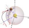 |
Fig. 1 Geometry of the model studied by Ershova & Schmidt (2021) transferred to the heliocentric coordinate system. The vector v⊥ is the projection of vector v onto the plane tangential to the sphere centered at the Sun and that contains the position of the source on the asteroid, located at position rM. The remaining variables are defined in Table 1. |
2.1 Radiation pressure
Considering the dust grains’ dynamics as a two-body problem with the Sun as the main gravitating body allows us to take into account the force exerted by solar radiation pressure without changing the dynamical equations. Namely, solar gravity and radiation pressure are both central forces decreasing with the inverse square of the heliocentric distance. Hence, the particle motion can be considered within the two-body problem using a reduced gravitational parameter as if the Sun had a lower mass. We define the reduced gravitational parameter as
![$\[\mu_{R}=G M_{S~un}(1-\beta(R))\]$](/articles/aa/full_html/2025/01/aa52162-24/aa52162-24-eq1.png) (1)
(1)
for particles of radius R, where G is the universal gravitational constant, MS un is the solar mass and β(R) is the ratio of the radiation pressure force to the gravitational force (Burns et al. 1979) computed as
![$\[\beta=\frac{3 L_{S ~un}}{16 \pi c ~G M_{S ~un}} \frac{Q_{p r}}{\rho R}.\]$](/articles/aa/full_html/2025/01/aa52162-24/aa52162-24-eq4.png) (2)
(2)
Here ρ denotes the bulk density of the dust grain, LS un is the Sun’s luminosity, c stands for the speed of light, R is the particle radius, and Qpr is the radiation pressure efficiency averaged over solar spectrum, which generally depends on particle size, shape, and material.
In addition to the Keplerian orbits considered in Ershova & Schmidt (2021), the case of a repulsive force may arise when we take into account radiation pressure. The parameter μR becomes negative if the acceleration due to radiation pressure is larger than solar gravity acceleration (β > 1). Geometrically in this case dust grains are moving along the hyperbola’s branch that lies on the other side of the hyperbola’s center than the Sun. We generalized the solution of Ershova & Schmidt (2021) to account for the repulsive force case utilizing the analogue of Kepler’s equation for the motion under a repulsive force that is scaling with inverse square of distance from the Sun (see, e.g., Hui 2023).
Definition of variables.
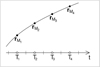 |
Fig. 2 Moving dust source represented by many sources placed along the given trajectory. Each of these sources is active for a short or infinitely small period of time around Tj. |
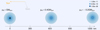 |
Fig. 3 Prime dust clouds ejected by a point source at the same time. The direction of the asteroid motion (apex) is shown relative to the direction toward the Sun. The cross sections of number density (m−3) in the orbital plane of the source are shown at 50 minutes after ejection. The black dot indicates the position of the asteroid center at the same time. The total number of dust particles in each prime cloud is the same (105 grains) with fixed grain sizes that correspond in each case to values of the parameter μR of GMS un, 0.4GMS un, −0.2GMS un, which determines the dust dynamics. The centers of these prime clouds lie on a synchrone. |
2.2 Model dust cloud formation
Let us call the spatial configuration of dust from one model source a “prime dust cloud.” All the particles in a prime cloud are affected by practically the same total force. If we take into account only the solar gravity and radiation pressure, then different values of Tj and μR correspond to different prime clouds. The prime clouds are the building blocks of our model for actual physical dust clouds around asteroids. The number density of dust at any point is a sum of the number densities of dust from all the prime clouds overlapping at this point. Additionally, we introduce the concept of the “center of a prime cloud,” which represents the position of a hypothetical particle ejected from the source with zero velocity and that moves under the influence of the same forces acting on the entire prime cloud (neglecting physical obstacles). It is important to note that prime clouds are not necessarily symmetrical, meaning the center of a prime cloud, as defined here, may not coincide with the cloud’s center of mass.
In this section, we consider how the model dust cloud is formed as a superposition of prime clouds. This allows us to estimate how many prime clouds one must take into account for the calculation of the dust number density at the given point for achieving a desired accuracy.
Let us consider one prime cloud ejected by an asteroid represented by one point source, with uniformly distributed directions and ejection speed distributed uniformly between umin and umax. All dust particles shall have the same size, and so the same μR. If we consider the prime cloud motion only for a short time after ejection, deviations from spherical symmetry of this prime cloud can be neglected. The prime cloud can be said to grow uniformly with time, as it is very small compared to its distance from the Sun, and so the forces of solar gravity and radiation pressure are practically the same for all the dust grains in the cloud. The dust ejected in this way forms a cloud limited by two spherical shells with radii of uminΔt and umaxΔt. With time dust is redistributed within the expanding spherical layer between uminΔt and umaxΔt so that its density decreases. The trajectory of the prime dust cloud center is determined by the parameter μR as well as the source position and velocity vectors at the time of creation of the cloud.
The centers of the prime clouds that are ejected at the same time, though that may differ in μR, evolve on a line called a synchrone (Finson & Probstein 1968a). Figure 3 shows a cross section of three prime clouds in the orbital plane of the asteroid. Each of the prime clouds contains 105 dust grains (an arbitrary chosen normalization factor). We adapt the values of umin = 2 m/s and umax = 30 m/s. The dust is ejected at approximately 0.16 AU heliocentric distance on the asteroid’s outbound orbit. At this proximity to the Sun the difference in dynamics due to the effect of radiation pressure (different for different μR) accumulates quickly. The dust spatial distribution is shown 50 minutes after the time of ejection for three prime clouds with μR equal to GMS un, 0.4GMS un, and −0.2GMS un, corresponding to β = 0, 0.6, 1.2, respectively. The leftmost cloud in Fig. 3 experiences zero radiation pressure (which can be a valid approximation for large dust grains), and so this prime cloud stays symmetrical around the asteroid at its center. The dust moves away from the center, and after a sufficiently long time, this dust leaves the given vicinity of the asteroid. One can roughly estimate the prime cloud center distance from the asteroid’s which is the origin of the coordinate system in Figs. 3 and 4 as
![$\[\Delta d=\frac{(G M_{S~un}-\mu_{R})\Delta t^{2}}{2 r_{M}^{2}},\]$](/articles/aa/full_html/2025/01/aa52162-24/aa52162-24-eq5.png) (3)
(3)
considering the source’s heliocentric distance rM constant for the approximation. Knowing the position of a point of interest r relative to the position of the asteroid, one can check if that point lies inside the prime cloud before computing this prime cloud’s contribution to the number density.
Centers of the prime clouds ejected at different times but having the same parameter μR lie on a line called a syndyne (Finson & Probstein 1968a). Figure 4 shows three prime clouds on a syndyne or, in other words, the time evolution of a prime cloud in the orbital plane of the source. The three prime clouds contain the same total number of particles (105 grains), have the same ejection parameters and the same value of μR = 0.5GMS un but they were ejected at three times Tj separated by 30 min from each other. Thus, we see that a prime cloud grows with time, becoming less dense, and, if having μR < GMS un, separates from its source. Let the total number of dust grains in a prime cloud be equal to Γ. This number is conserved in the evolution of the cloud after ejection. Therefore, the maximum number density within a prime cloud can be estimated through the maxima of the dust ejection parameters distributions multiplied by a factor accounting for the expansion of the prime cloud with time (more details about this factor are given in Sect. 2.6). Here this factor is Δt(uΔt)2, and the estimation reads
![$\[n_{max} \leq {max} \left(\frac{f_{u}}{(u \Delta t)^{2}}\right) \frac{\Gamma ~{max}(f_{\tilde{\psi}, {\tilde{\lambda}_{M}}})}{\Delta t},\]$](/articles/aa/full_html/2025/01/aa52162-24/aa52162-24-eq6.png) (4)
(4)
where fu is the distribution of the particles’ ejection speed u, and ![$\[f_{\tilde{\psi}, \tilde{\lambda}_{M}}\]$](/articles/aa/full_html/2025/01/aa52162-24/aa52162-24-eq7.png) is the distribution of ejection directions. Defining a lower limit for nmax we can find Δt for which performing calculations is unnecessary (i.e., the prime dust cloud was ejected a sufficiently long time ago such that at time of interest tnow it is already negligibly sparse).
is the distribution of ejection directions. Defining a lower limit for nmax we can find Δt for which performing calculations is unnecessary (i.e., the prime dust cloud was ejected a sufficiently long time ago such that at time of interest tnow it is already negligibly sparse).
In the close proximity to the asteroid, as shown in Figs. 3 and 4, syndynes and synchrones are practically indistinguishable, and, roughly speaking, for β > 0 the prime clouds separate from the asteroid along the continuation of its heliocentric position vector. Orbital phase lag relative to the asteroid accumulates more slowly than the radial distance.
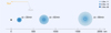 |
Fig. 4 Prime dust clouds ejected by a point source at three different times. The direction of the asteroid motion (apex) is shown relative to the direction toward the Sun. Each prime cloud contains 105 dust particles. The cross section of particle number density (m−3) in the orbital plane of the source is shown 30 minutes (left) after ejection, 60 minutes (middle), and 90 minutes (right). The black dot indicates the position of the asteroid 90 minutes after the first prime cloud was ejected. All particles in the three prime clouds are of the same size corresponding to μR = 0.5GMS un. The centers of these prime clouds lie on a syndyne. |
2.3 Adapting the model by Ershova & Schmidt (2021) for a moving object
According to Ershova & Schmidt (2021), if the dust is ejected from a point rM with a time-dependent production rate γ(t), then the expression for the number density of dust particles with radii within the range (Rmin, Rmax) at the time tnow at point r is
![$\[\begin{aligned}& n(\mathbf{r}, R_{min}<R<R_{max}, t_{now}) \\& \quad=\frac{1}{r r_M ~\sin~ \Delta \phi} \int_{R_{min}}^{R_{max }} \mathrm{d} R ~f_R(R) \int_{v_{min}}^{v_{\max }} \mathrm{d} v \frac{v}{u^2} \\& \qquad \times \sum_i \gamma(t_{now}-\Delta t_i) \frac{f_{u, \psi, \lambda_M}(u, \psi_i, \lambda_{M i}) ~\sin~ \psi_i}{\cos~ \psi_i}\left|\frac{\partial \Delta \phi}{\partial \theta~_{\theta_i}}\right|^{-1}.\end{aligned}\]$](/articles/aa/full_html/2025/01/aa52162-24/aa52162-24-eq8.png) (5)
(5)
Variables are defined in Fig. 1 and Table 1 (see also Ershova & Schmidt 2021). The sum under the integral accounts for possible trajectories a dust particle can take from the source position rM to the spacecraft position r with a velocity v. The trajectories are found from the equations of the two-body problem for given gravitational parameter, which, taking into account the effect of radiation pressure, is replaced by the reduced gravitational parameter μR, depending on the particle radius R. Thus, the integral over v implicitly depends on the dust grain size. The position vectors are defined in a coordinate system (Fig. 1) centered in the gravitating body (the Sun) which can be treated as a point mass. The angle Δϕ is between r and rM. The function fR(R) is the distribution of particle radii (R) of the emitted dust normalized in (Rmin, Rmax). At the point r a particle’s speed is denoted by v and the angle between the particle velocity and position vectors is denoted by θ; ψ is the zenith angle of the particle ejection velocity, and λM is the azimuth of this vector.
To solve this problem, we considered four coordinate systems in which we can express the phase space coordinates of the dust grains and the asteroid itself (see Fig. 5). The coordinate system centered at the gravitational field source, which, in our case, is the Sun is denoted as S in Fig. 5. The source and the spacecraft coordinates are defined in the system S. The velocity vector components of the dust particle at the time of its ejection (u, ψ, λM) are expressed in the inclined heliocentric system ![$\[\tilde{S}\]$](/articles/aa/full_html/2025/01/aa52162-24/aa52162-24-eq9.png) . This system
. This system ![$\[\tilde{S}\]$](/articles/aa/full_html/2025/01/aa52162-24/aa52162-24-eq10.png) has its z-axis aligned with the source’s heliocentric radius vector, and the x-axis of the system
has its z-axis aligned with the source’s heliocentric radius vector, and the x-axis of the system ![$\[\tilde{S}\]$](/articles/aa/full_html/2025/01/aa52162-24/aa52162-24-eq11.png) is parallel to the direction of the local north of the system S at the source position in the time of dust ejection (along the projection of the z-axis onto the plane tangential to the Sun-centered sphere of radius rM at the source position rM). The coordinate system A has its axes parallel to the axes of
is parallel to the direction of the local north of the system S at the source position in the time of dust ejection (along the projection of the z-axis onto the plane tangential to the Sun-centered sphere of radius rM at the source position rM). The coordinate system A has its axes parallel to the axes of ![$\[\tilde{S}\]$](/articles/aa/full_html/2025/01/aa52162-24/aa52162-24-eq12.png) but is centered at the position of the dust source at the time of ejection. It moves with the velocity of the source. This velocity is considered constant, having the value assumed by the source at the time of dust ejection.
but is centered at the position of the dust source at the time of ejection. It moves with the velocity of the source. This velocity is considered constant, having the value assumed by the source at the time of dust ejection.
The distributions of ejection speed and direction are more straightforwardly described in the inclined system ![$\[\tilde{A}\]$](/articles/aa/full_html/2025/01/aa52162-24/aa52162-24-eq13.png) moving with the asteroid in the same manner as the system A but having its polar axis
moving with the asteroid in the same manner as the system A but having its polar axis ![$\[\tilde{Z}\]$](/articles/aa/full_html/2025/01/aa52162-24/aa52162-24-eq14.png) aligned with the ejection axis of symmetry. In the model published by Ershova & Schmidt (2021), describing dust emission from a gravitating spherical moon, this system tilted relative to the position vector of the source was stationary, and ejection was only possible toward the positive direction of the axis Z of system A (i.e., directed into the half space radially outward from the dust emitting surface). In this paper, we overcome this restriction, allowing the ejection symmetry axis
aligned with the ejection axis of symmetry. In the model published by Ershova & Schmidt (2021), describing dust emission from a gravitating spherical moon, this system tilted relative to the position vector of the source was stationary, and ejection was only possible toward the positive direction of the axis Z of system A (i.e., directed into the half space radially outward from the dust emitting surface). In this paper, we overcome this restriction, allowing the ejection symmetry axis ![$\[\tilde{Z}\]$](/articles/aa/full_html/2025/01/aa52162-24/aa52162-24-eq15.png) to point in any direction. This enables us to model dust ejection from the entire surface of the asteroid including those surface elements facing the Sun, which is the center of gravity.
to point in any direction. This enables us to model dust ejection from the entire surface of the asteroid including those surface elements facing the Sun, which is the center of gravity.
In Eq. (5), the velocity vector components of the dust grain at the point r, which are (v, θ, λ), are expressed in a coordinate system defined in a manner as the system ![$\[\tilde{S}\]$](/articles/aa/full_html/2025/01/aa52162-24/aa52162-24-eq16.png) but centered in the point r instead of rM. Here the
but centered in the point r instead of rM. Here the ![$\[\tilde{z}\]$](/articles/aa/full_html/2025/01/aa52162-24/aa52162-24-eq17.png) -axis points along the spacecraft radius-vector and the
-axis points along the spacecraft radius-vector and the ![$\[\tilde{x}\]$](/articles/aa/full_html/2025/01/aa52162-24/aa52162-24-eq18.png) -axis along the local north defined at the point r at time tnow.
-axis along the local north defined at the point r at time tnow.
We define the distributions of ejection speed ![$\[f_{u^{\tilde{A}}}(u^{\tilde{A}})\]$](/articles/aa/full_html/2025/01/aa52162-24/aa52162-24-eq22.png) and direction
and direction ![$\[f_{\psi^{\tilde{A}}, \lambda_{M}^{\tilde{A}}}(\psi^{\tilde{A}}, \lambda_{M}^{\tilde{A}})\]$](/articles/aa/full_html/2025/01/aa52162-24/aa52162-24-eq23.png) in the system
in the system ![$\[\tilde{A}\]$](/articles/aa/full_html/2025/01/aa52162-24/aa52162-24-eq24.png) . To obtain the solution to Eq. (5), we need to establish a connection between this system and the system
. To obtain the solution to Eq. (5), we need to establish a connection between this system and the system ![$\[\tilde{S}\]$](/articles/aa/full_html/2025/01/aa52162-24/aa52162-24-eq25.png) , where we express the ejection velocity vector over which we integrate to obtain the number density of dust. The Jacobian Jtilt for the transformation from the system A to the system
, where we express the ejection velocity vector over which we integrate to obtain the number density of dust. The Jacobian Jtilt for the transformation from the system A to the system ![$\[\tilde{A}\]$](/articles/aa/full_html/2025/01/aa52162-24/aa52162-24-eq26.png) was provided in previous work (see Fig. 2 in Ershova & Schmidt 2021). For modeling dust ejection from a moving object we must derive a Jacobian Jmotion to perform an additional coordinate transformation (between the systems A and
was provided in previous work (see Fig. 2 in Ershova & Schmidt 2021). For modeling dust ejection from a moving object we must derive a Jacobian Jmotion to perform an additional coordinate transformation (between the systems A and ![$\[\tilde{S}\]$](/articles/aa/full_html/2025/01/aa52162-24/aa52162-24-eq27.png) ) to account for the source velocity V. This velocity should be understood as a velocity of a surface element where the dust is ejected from. In practice, we treat it as the velocity of the asteroid center, though the vector V can also be adjusted to account for the asteroid’s rotation. The Jacobians for both transformations are given in Appendix A. Thus,
) to account for the source velocity V. This velocity should be understood as a velocity of a surface element where the dust is ejected from. In practice, we treat it as the velocity of the asteroid center, though the vector V can also be adjusted to account for the asteroid’s rotation. The Jacobians for both transformations are given in Appendix A. Thus,
![$\[\begin{aligned}& f_{u, \psi, \lambda_M}(u, \psi, \lambda_M) ~\sin~ \psi \\& \quad=f_{u^A, \psi^A, \lambda_M^A}(R, u^A, \psi^A, \lambda_M^A) ~\sin~ \psi^A|J_{motion}| \\& \quad=|J_{tilt} \| J_{motion}| f_{u^{\tilde{A}}}(u^{\tilde{A}}, R) f_{\psi^{\tilde{A}}, \lambda_M^{\tilde{A}}}(\psi^{\tilde{A}}, \lambda_M^{\tilde{A}}) ~\sin~ \psi^{\tilde{A}}.\end{aligned} \]$](/articles/aa/full_html/2025/01/aa52162-24/aa52162-24-eq28.png) (6)
(6)
In what follows we describe three methods to evaluate the integral in Eq. (5) for a time dependent dust production rate γ(t). The choice of the best suited solution method for a given problem depends on the asteroid orbital parameters and the time passed since ejection, Δt. The integration over the grain radius R has to be the last step in the evaluation of the Eq. (5) because the particle size determines the parameter μR, and thus the solution of the dynamical problem.
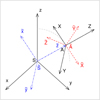 |
Fig. 5 Position vectors of dust source rM and spacecraft r (in spherical coordinates (rM, αM, ωM) and (r, α, ω), respectively), defined in the Suncentered system S (compare to Fig. 1). The particle velocity vector at the time of ejection (u, ψ, λM) is defined in the coordinate system |
![$\[\tilde{S}\]$](/articles/aa/full_html/2025/01/aa52162-24/aa52162-24-eq19.png)
![$\[\tilde{S}\]$](/articles/aa/full_html/2025/01/aa52162-24/aa52162-24-eq20.png)
![$\[\tilde{A}\]$](/articles/aa/full_html/2025/01/aa52162-24/aa52162-24-eq21.png)
2.4 The v-integration method
The v-integration method obtains the number density of the dust ejected by a moving source from Eq. (5) upon numerical integration over particle velocities. This method assumes that the sources placed along the trajectory eject dust over a short time interval Δτ. This interval must be less than or equal to (Tj+1 − Tj), the difference between neighboring times Tj (see Fig. 2). As an approximation, we consider the positions of the dust sources to be unchanged over this time interval. However, the dust grains leave the asteroid having a velocity of ![$\[\mathbf{u}=\mathbf{V}+\mathbf{u}^{\tilde{A}}\]$](/articles/aa/full_html/2025/01/aa52162-24/aa52162-24-eq29.png) , so that the asteroid’s motion itself is taken into account. The v-integration method is applicable to any Δt shorter than half of the orbital period. However, also for small Δt, this method may encounter numerical problems caused by the proximity to the degenerate case Δϕ = 0 described in Ershova & Schmidt (2021).
, so that the asteroid’s motion itself is taken into account. The v-integration method is applicable to any Δt shorter than half of the orbital period. However, also for small Δt, this method may encounter numerical problems caused by the proximity to the degenerate case Δϕ = 0 described in Ershova & Schmidt (2021).
The asteroid velocity is much higher than the dust grains’ ejection velocities. Therefore, the asteroid velocity can be considered an approximate solution for the particles’ velocities and the actual solution is searched for close to this value. This allowed us, when following the algorithm of Ershova & Schmidt (2021), to remove from consideration those dust trajectories that appear in course of solving the mathematical problem but differ drastically from the asteroid trajectory.
Calculating the limits of integration (vmin, vmax) in the same way as for a motionless source (Ershova & Schmidt 2021) provides too loose bounds for the case of a moving source. This is because the limits were computed from the orbital energy, while the time needed for traveling from rM to r was not taken into account. Knowing the time (Tj − Δτ/2, Tj + Δτ/2) when the source is active, we could narrow down the corresponding interval of velocities ![$\[\left(v_{min}^{*}, v_{max}^{*}\right)\]$](/articles/aa/full_html/2025/01/aa52162-24/aa52162-24-eq30.png) . Then we integrate over
. Then we integrate over ![$\[\left(v_{min}^{*}, v_{max}^{*}\right)\]$](/articles/aa/full_html/2025/01/aa52162-24/aa52162-24-eq31.png) ⊂ (vmin, vmax). Furthermore, with a fixed Δt, there is only one path that a particle can take from the source to the spacecraft position. Consequently, the summation in Eq. (5) is unnecessary when considering a moving object. Thus, the formula for the v-integration solution is
⊂ (vmin, vmax). Furthermore, with a fixed Δt, there is only one path that a particle can take from the source to the spacecraft position. Consequently, the summation in Eq. (5) is unnecessary when considering a moving object. Thus, the formula for the v-integration solution is
![$\[\begin{aligned}& n\left(\mathbf{r}, R, t_{now}\right) \\&\quad = \frac{f_R(R)}{r r_M ~\sin~ \Delta \phi} \int_{v_{min }}^{v_{max }^*} \mathrm{~d} v \frac{v}{u^2} \gamma\left(t_{now}-\Delta t\right) \\& \\& \qquad ~\times \frac{f_{u, \psi, \lambda_M}(u, \psi, \lambda_M) ~\sin~ \psi}{\cos~ \psi}\left|\frac{\partial \Delta \phi}{\partial \theta~_\theta}\right|^{-1}.\end{aligned}\]$](/articles/aa/full_html/2025/01/aa52162-24/aa52162-24-eq32.png) (7)
(7)
2.5 The δ-ejection method
The δ-ejection method assumes that sources are active only for an infinitely small interval of time. In this case, integration over v can be performed analytically and the computational effort is reduced significantly. The δ-ejection method is applicable for sufficiently small time intervals since ejection because it relies on the Taylor expansion by Δt.
We defined the time dependent production rate of a given source as
![$\[\gamma(t)=\Gamma \delta\left(t-T_{j}-\Delta t\right).\]$](/articles/aa/full_html/2025/01/aa52162-24/aa52162-24-eq33.png) (8)
(8)
Then there exists only one value of vector u that corresponds to a particle traveling from rM to r exactly in the time Δt = tnow − Tj. Performing a replacement of the variable in the argument of the δ-function and then integrating over v, we obtained the solution
![$\[\begin{aligned}n(\mathbf{r}, R, t)= & \frac{\Gamma}{r r_M} \frac{v\left(u^*\right)}{u^2 ~\sin~ \alpha_M} f_R(R) \\& \times \frac{f_{u, \psi, \lambda_M}\left(u^*, \psi^*, \lambda_M^*\right) ~\sin~ \psi^*}{\cos ~\psi^*}\left|\frac{\partial\left(\Delta t, \alpha_M, \omega_M\right)}{\partial(v, \theta, \lambda)}\right|_{\mathbf{r}}^{-1}.\end{aligned}\]$](/articles/aa/full_html/2025/01/aa52162-24/aa52162-24-eq34.png) (9)
(9)
Here, the variables with an asterisk denote those particular values of the velocity vector components that are required for a dust grain to travel from rM to r in time Δt.
The azimuth λ, measured clockwise from the local north, determines the orientation of the particle’s orbital plane in the coordinate system ![$\[\tilde{S}\]$](/articles/aa/full_html/2025/01/aa52162-24/aa52162-24-eq35.png) but is unrelated to the energy and shape of the orbit. Therefore, ∂Δt/∂λ = 0 and the Jacobian in Eq. (9) reads
but is unrelated to the energy and shape of the orbit. Therefore, ∂Δt/∂λ = 0 and the Jacobian in Eq. (9) reads
![$\[\left|\frac{\partial\left(\Delta t, \alpha_{M}, \omega_{M}\right)}{\partial(v, \theta, \lambda)}\right|_{\mathbf{r}}=\left|\frac{\sin \Delta \phi}{\sin \alpha_{M}}\left(\frac{\partial \Delta t}{\partial v} \frac{\partial \Delta \phi}{\partial \theta}-\frac{\partial \Delta t}{\partial \theta} \frac{\partial \Delta \phi}{\partial v}\right)\right|.\]$](/articles/aa/full_html/2025/01/aa52162-24/aa52162-24-eq36.png) (10)
(10)
To evaluate this formula, we must compute the components of the velocity vectors, namely ![$\[u^{*}, \psi^{*}, \lambda_{M}^{*}, v^{*}, \theta^{*}\]$](/articles/aa/full_html/2025/01/aa52162-24/aa52162-24-eq37.png) , assuming that the distance from the source to the spacecraft position and the time of flight between these two points are small on the scales of the asteroid orbit.
, assuming that the distance from the source to the spacecraft position and the time of flight between these two points are small on the scales of the asteroid orbit.
The velocity azimuth angle λM can be calculated as the angle between the direction to the local north (N) and the vector pointing from rM to r (see Fig. 1).
To obtain u* and θ*, we considered a coordinate plane centered at the Sun, which coincides with the dust grain’s orbital plane, with the x-axis pointing along rM. In this coordinate system, for the position of the spacecraft is given by
![$\[\mathbf{r}=(x, y), x=r ~\cos~ \Delta \phi, ~y=r ~\sin~ \Delta \phi,\]$](/articles/aa/full_html/2025/01/aa52162-24/aa52162-24-eq38.png) (11)
(11)
and the position of the dust source is
![$\[\mathbf{r}_{M}=\left(r_{M}, 0\right).\]$](/articles/aa/full_html/2025/01/aa52162-24/aa52162-24-eq39.png) (12)
(12)
Taking into account that both components of the vector r − rM are very small compared to the heliocentric distances r and rM, we approximated x and y with a Taylor polynomial
![$\[\begin{aligned}x \approx & r_M+u_x \Delta t+\frac{a_x \Delta t^2}{2} \\& +\frac{\dot{a}_x \Delta t^3}{6}+\frac{\ddot{a}_x \Delta t^4}{24}+\frac{a_x^{(3)} \Delta t^5}{120}+\frac{a_x^{(4)} \Delta t^6}{720},\end{aligned}\]$](/articles/aa/full_html/2025/01/aa52162-24/aa52162-24-eq40.png) (13)
(13)
![$\[y \approx u_y \Delta t+\frac{\dot{a}_y \Delta t^3}{6}+\frac{\ddot{a}_y \Delta t^4}{24}+\frac{a_y^{(3)} \Delta t^5}{120}+\frac{a_y^{(4)} \Delta t^6}{720}.\]$](/articles/aa/full_html/2025/01/aa52162-24/aa52162-24-eq41.png) (14)
(14)
In the chosen coordinate system, the y components of rM and the acceleration vector are zero, and dr/dt = ux at the point rM. The expressions for the nonzero derivatives in Eqs. (13) and (14) are provided in Appendix B. These expressions are substituted into Eqs. (13) and (14) and then they are solved iteratively, using the radial and tangential components of the asteroid’s velocity as initial guesses for ux and uy, respectively. The quantities required for evaluating the number density are then
![$\[u^{*}=\sqrt{u_{x}^{2}+u_{y}^{2}}\]$](/articles/aa/full_html/2025/01/aa52162-24/aa52162-24-eq42.png) (15)
(15)
![$\[\psi^{*}=k \pi+\arctan \frac{u_{y}}{u_{x}},\]$](/articles/aa/full_html/2025/01/aa52162-24/aa52162-24-eq43.png)
where k = 0 if the asteroid is moving away from the Sun, and k = 1 if it is moving toward the Sun. The corresponding values of v and θ can be found from the conserved orbital energy, and angular momentum.
2.6 The simple expansion method
When computing the number density of recently ejected dust, one can employ an approximation that, although basic, is not limited to the effects of solar gravity and radiation pressure. We can determine the coordinates of the prime cloud center by direct integration of its trajectory. Then, assuming that a prime cloud is small relative to the gradient of the total force governing dust dynamics, we derived the spatial distribution of dust by multiplying the distribution of ejection parameters with the factor governing the expansion of the prime cloud around its center. This gives
![$\[n(\mathbf{r}, t_{now})=\frac{\Gamma}{\Delta t} \frac{f_{\psi, \lambda_{M}}(\psi, \lambda_{M}) f_{u}(u)}{|\mathbf{r}-\mathbf{r}_{c}|^{2}}, u=\frac{|\mathbf{r}-\mathbf{r}_{c}|}{\Delta t}.\]$](/articles/aa/full_html/2025/01/aa52162-24/aa52162-24-eq44.png) (17)
(17)
Here n is the dust number density at the point r at the time tnow, and rc is the position of the prime cloud center at this time. The factor Γ sets the total number of particles ejected by the source. The function fu(u) is the distribution of ejection speed (u); fψ, λM (ψ, λM) is the distribution of the ejection direction defined in terms of the zenith angle ψ and azimuth λM of the ejection velocity vector. The azimuth is measured clockwise from the local north.
A similar idea was implemented by Finson & Probstein (1968a), who represented comet tails as an ensemble of spheres formed by dust particles ejected at the same time with the same speed, and experiencing the same radiation pressure. The gradient of gravity and radiation pressure was neglected within one sphere.
We suggest that when using the simple expansion method to describe dust dynamics, any perturbations can be taken into account as long as they induce equal accelerations on all dust grains within the prime cloud. This condition is met not only by solar gravity and radiation pressure but also by plasma drag and the interplanetary magnetic field. Although the latter two exhibit irregular large-scale spatial variations, they can be regarded as constant over the scale of a single prime cloud.
To obtain the prime cloud center position rc, one must integrate the motion of one particle ejected by the model source with zero velocity. This particle separates from the asteroid at the time Tj and possibly starts experiencing forces that are negligible for the parent body. This solution however neglects the physical shape of the parent body of the dust, as the dust is assumed to be ejected from a single point source, and the curvature of its orbit is neglected, because the direction of the ejection velocity vector is considered constant after ejection.
3 DUDI-heliocentric
The methods described in the previous sections have been implemented as a Fortran-95 software package named DUDI-heliocentric1 (where DUDI stands for “dust distribution”). It inherits the structure of the package DUDI (Ershova & Schmidt 2021), though the main routines were implemented anew. This was necessary because the three solution methods (v-integration (see Sect. 2.4), δ-ejection (Sect. 2.5), and simple expansion (Sect. 2.6) methods) employ algorithms significantly different from the method of Ershova & Schmidt (2021).
Like DUDI (Ershova & Schmidt 2021), DUDI-heliocentric accepts as input parameters the time at which the number density must be computed (tnow) and the coordinates of the point of interest (r), the dust source (rM), and the form and parameters of the distributions of ejection speed and direction, describing the dynamical parameters of ejection. Additionally, the time when the source is active (Tj − Δτ/2, Tj + Δτ/2) and the reduced gravitational parameter (μR) used in calculations must be specified. In contrast to the original DUDI, DUDI-heliocentric produces output for a given grain size which is fixed by setting the parameter μR. Results for a given size distribution are obtained by a proper average of the output for individual grain sizes. Instead of the dust ejection rate (γ), as used in the original DUDI, DUDI-heliocentric takes as input the total number of particles (Γ) ejected by the source. The concept of production rate has a physical meaning only if the v-integration method is chosen; in this case, the production rate is considered constant over the time of the source activity (γ = Γ/Δτ).
To improve the numerical stability of the calculations, in DUDI-heliocentric we express distances in AU and velocities in AU/day in all calculations. However, the computed number density is expressed in m−3 for convenience. Care must be taken when defining a customized distribution of particle ejection speed, as this function receives ejection speed in AU/day as its argument and must return the result in day/AU. Typically, it is more convenient to define such a distribution using parameters expressed in the International System of Units (SI), as we do it in the following Sect. 4. In this case, the user must convert the units before computing the value of the function, and the function’s result must be expressed in the correct units.
We developed a procedure that allows us to account for the re-impacts of ejected particles with their parent body when using the v-integration or δ-ejection method and representing the asteroid with numerous sources (typically hundreds) distributed across its surface. For this, the asteroid’s shape is assumed to be spherical, and the radius of this sphere is provided as an additional input parameter in DUDI-heliocentric. Details of the algorithm are described in Appendix C.
In this section, we outline the tests conducted to verify the correct performance of DUDI-heliocentric and provide general guidelines for code users. These guidelines pertain only to the applicability limits of the code and the selection of the appropriate solution method among the three available options. For detailed instructions on how to use DUDI-heliocentric, we refer to the README.md file on GitHub.
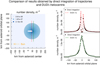 |
Fig. 6 Comparison of DUDI-heliocentric to results obtained by the direct integration of trajectories. The dust cloud in the left panel, obtained with DUDI-heliocentric, is shown in the plane normal to the asteroid orbital plane and containing the asteroid’s instantaneous heliocentric position vector. The dust was ejected 15 min before tnow from 2000 sources uniformly distributed on the surface of a spherical asteroid with 5 km radius. Radiation pressure is considered, with β set to 0.5, and dust grain re-collisions with the asteroid are taken into account. The lines in the left panel represent the cuts for which number densities are displayed in the right panel. |
3.1 Code performance evaluation
We validated the performance of DUDI-heliocentric comparing to the results obtained with a well tested code that evaluates dust number densities by direct integration of the dynamical equations for dust grains (Liu et al. 2016; Liu & Schmidt 2018, 2019, 2021; Yang et al. 2022; Chen et al. 2024). The direct integrations are numerically expensive but they can in principle resolve the full physics of grain dynamics, including nongravitational perturbation forces, like the Lorentz force exerted by the interplanetary magnetic field on charged particles. Figure 6 shows the comparison of a dust cloud evaluated with the two software packages. Profiles and the cross section are shown for the number density of dust ejected from 2000 point sources uniformly distributed on the surface of a spherical asteroid with 5 km radius. The model asteroid was moving on the orbit of NEA 3200 Phaethon. Dust is ejected at 0.16 AU heliocentric distance, soon after the asteroid passed its perihelion. Each of the 2000 sources ejects 2 × 10⁵ particles instantaneously with ejection directions distributed uniformly within a cone of 60° full opening angle, and ejection velocities uniformly distributed between 0 and 100 m/s. The profiles are shown for the dust configuration 15 min after the time of ejection. We considered the radiation pressure force with β = 0.5 and accounted for particles re-colliding with the asteroid when ejected toward the Sun and then pushed back by the radiation pressure (see Appendix C). This results in the formation of an empty hollow inside the cloud. Each point on the profile obtained from the trajectory integration code is an average over a grid cell of a given volume, whereas the number density evaluated by DUDI-heliocentric is a continuous function. This accounts for the differences in the profile shown in the upper panel that manifest at the edges of the dust-free region in the middle of the cloud.
DUDI-heliocentric obtained the cloud shown in Fig. 6 within a few CPU seconds on a 4-cored laptop (where the δ-ejection method was used) while the trajectory code utilized several hours on a computer cluster using 256 cores. Moreover, the CPU time required by the trajectory code scales with the time after dust ejection Δt. The computational time for the δ-ejection and v-integration methods of DUDI-heliocentric does not depend on Δt. The simple expansion method involves an integration of the trajectories of the prime clouds’ centers. Hence, this method requires in principle longer calculations for larger Δt, too. But the applicability of the method is limited to short intervals Δt anyway, so an enhanced demand on CPU time does not manifest in practice. The δ-ejection method’s accuracy degrades for large Δt; however, the divergence is sufficiently slow for this method so that it remains applicable to a wide range of problems.
We further tested DUDI-heliocentric by comparing the three methods against each other. Specifically, we investigated how the asteroid’s orbital parameters influence the accuracy of the δ-ejection method, which employs a Taylor expansion of the dynamical equations in powers of the time Δt elapsed since the time of ejection (see Sect. 2.5). The accuracy of this method was assessed by comparing it to the results obtained with the v-integration method, which accounts for the dynamics of the two-body problem without simplifications. We compared the outcomes of the two methods across several representative scenarios of dust ejection, including dust ejection from comet C/2011 W3 (Lovejoy) shortly before its perihelion passage, C/2011 W3 (Lovejoy) at a distance of 0.5 AU on its outbound orbit, NEA 3200 Phaethon at a heliocentric distance of 0.16 AU shortly after its perihelion passage, and NEA 3200 Phaethon at a heliocentric distance of 1 AU as it moves toward the Sun. To assess the accuracy of the solution, we varied parameters such as μR, Δt, and the time interval of the source activity (Δτ) for the v-integration method. In this way, we gained insight into the performance of each method under different conditions.
The v-integration method converges to the δ-ejection solution with decreasing time interval of dust ejection Δτ; however, Δτ must be greater than zero by the assumption of the v-integration method. The threshold of Δτ necessary to obtain a desired accuracy varies with the orbital velocity and the spacecraft position relative to the dust cloud. Those points of interest that require a very small ejection velocity ![$\[(u^{\widetilde{A}})\]$](/articles/aa/full_html/2025/01/aa52162-24/aa52162-24-eq45.png) to be reached by a particle, demand a smaller value of Δτ to accurately compute the dust density. In our tests with the asteroid Phaethon, we did not observe any drawbacks of selecting Δτ smaller than the value, which is sufficient for the convergence. However, for the extremely eccentric orbit of C/2011 W3 (Lovejoy), setting a too small Δτ led to numerical difficulties. When we computed the integrand in Eq. (7) the difference between the values at each integration step was below computational accuracy. This resulted in insufficient resolution for accurate computation of the dust density. Figure 7 illustrates this problem. Here we present two cross sections through a prime dust cloud that was ejected by a point source on the orbit of comet Lovejoy at a distance of 0.5 AU from the Sun, 20 hours before tnow. The ejection occurs uniformly in all directions, with ejection speeds uniformly distributed between 0.05 and 100 m/s. For this trajectory of the parent body and the time elapsed since the ejection, both the δ-ejection and v-integration methods are applicable. Therefore, we could utilize the profile of the δ-ejection solution as a reference for analyzing the choice of Δτ. The profile depicted in the upper panel Fig. 7 lies in the source orbital plane and traverses the very center of the dust cloud. In this profile, we observe that smaller value of Δτ results in a better resolution of the dust cloud center. However, in the lower panel of Fig. 7, which displays the profile normal to the orbital plane, passing as far from the prime cloud center as 20 km, we see that employing the same small value of Δτ leads to irregular fluctuations in the profiles, while a larger Δτ produces a less wiggled profile that also remains closer to the reference from the δ-ejection method.
to be reached by a particle, demand a smaller value of Δτ to accurately compute the dust density. In our tests with the asteroid Phaethon, we did not observe any drawbacks of selecting Δτ smaller than the value, which is sufficient for the convergence. However, for the extremely eccentric orbit of C/2011 W3 (Lovejoy), setting a too small Δτ led to numerical difficulties. When we computed the integrand in Eq. (7) the difference between the values at each integration step was below computational accuracy. This resulted in insufficient resolution for accurate computation of the dust density. Figure 7 illustrates this problem. Here we present two cross sections through a prime dust cloud that was ejected by a point source on the orbit of comet Lovejoy at a distance of 0.5 AU from the Sun, 20 hours before tnow. The ejection occurs uniformly in all directions, with ejection speeds uniformly distributed between 0.05 and 100 m/s. For this trajectory of the parent body and the time elapsed since the ejection, both the δ-ejection and v-integration methods are applicable. Therefore, we could utilize the profile of the δ-ejection solution as a reference for analyzing the choice of Δτ. The profile depicted in the upper panel Fig. 7 lies in the source orbital plane and traverses the very center of the dust cloud. In this profile, we observe that smaller value of Δτ results in a better resolution of the dust cloud center. However, in the lower panel of Fig. 7, which displays the profile normal to the orbital plane, passing as far from the prime cloud center as 20 km, we see that employing the same small value of Δτ leads to irregular fluctuations in the profiles, while a larger Δτ produces a less wiggled profile that also remains closer to the reference from the δ-ejection method.
The simple expansion method requires even less CPU time than the δ-ejection method. However, it neglects the curvature of the asteroid orbit and simplifies the consideration of the change in dust grain velocities over their path from the source to the spacecraft (see Sect. 2.6). Nevertheless, the accuracy of the simple expansion method may be sufficient for practical problems. For instance, in the case investigated in Sect. 4.1.1, where we examine the dust environment of NEA 3200 Phaethon, the simple expansion method produces practically the same results as the δ-ejection method.
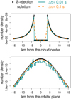 |
Fig. 7 Profiles of the spherically symmetric prime dust cloud ejected by a point source on the orbit of comet C/2011 W3 (Lovejoy) with e = 0.99993. The dust number density is evaluated 20 hours after the ejection. The profile in the upper panel lies in the source’s orbital plane and passes through the cloud center. This center has developed a hollow because of a nonzero minimum ejection velocity umin (see Sect. 2.2). The profile in the lower panel is normal to the source’s orbital plane, piercing this plane at 20 km distance from the cloud center. |
3.2 Guidelines for applying DUDI-heliocentric
Overall, the v-integration method has similar limitations as the DUDI code for a source at rest (Ershova & Schmidt 2021). Extra care must be taken when applying it to quasi-parabolic cases (0.998 < e < 1.001), trajectories close to the radial direction (ψ < 5° or ψ > 175°), and close to the model’s singularities, which are described in Section 2.4 of Ershova & Schmidt (2021). The other two methods do not require these conditions fulfilled because they do not rely on geometric calculations as the v-integration method and the original DUDI code for a source at rest.
Ershova & Schmidt (2021) describe in Section 3 that the integrand in Eq. (9) has a pole located at the minimal possible dust particle velocity at the spacecraft position r. However, this pole is not in practice encountered when using the v-integration method (see Eq. (7)) because the integration interval ![$\[\left(v_{min }^{*}, v_{max }^{*}\right)\]$](/articles/aa/full_html/2025/01/aa52162-24/aa52162-24-eq46.png) is very small, with values close to the asteroid velocity. The limits of integration
is very small, with values close to the asteroid velocity. The limits of integration ![$\[\left(v_{min}^{*}, v_{max}^{*}\right)\]$](/articles/aa/full_html/2025/01/aa52162-24/aa52162-24-eq47.png) are found iteratively by bisection, as the time Δt necessary for a particle to travel from the source to the spacecraft monotonically decreases with increasing particle velocity v.
are found iteratively by bisection, as the time Δt necessary for a particle to travel from the source to the spacecraft monotonically decreases with increasing particle velocity v.
In general, DUDI-heliocentric is unable to provide a solution if a particle passes perihelion between the time of ejection and the time it reaches the spacecraft because of an ambiguity arising in geometrical considerations of the cyclic variables as the true anomaly. However, the v-integration method of DUDI-heliocentric includes an option to handle such cases. It requires prior knowledge that the perihelion passage occurred, which must be provided as an input parameter (see README.md file for details). With this information, the v-integration algorithm can calculate the values of the angles between the particle position and velocity vectors at ejection (ψ) and at detection (θ), thereby yielding the correct solution for the dust density. However, at the very pericenter the angle ψ is equal to 90°, which corresponds to a zero in the denominator in Eq. (9). Therefore, numerical difficulty arises at those points of interest, where particles ejected very close to their perihelion contribute to the number density, which may cause a degradation of accuracy. What helps, is that such problematic points are located in different places for different prime clouds. If the desired result is a sum of number densities of dust from many prime clouds, the loss of accuracy is in general suppressed by the averaging. The δ ejection and the simple expansion methods are not recommended to use close to perihelion even if the time of perihelion passage itself lies outside the interval from the ejection to tnow because particles’ trajectories near the perihelion are highly curved. We note that the time of perihelion passage and the perihelion position of the asteroid and the ejected dust grains differ, though only slightly, because radiation pressure affects the dust but not the source. The information about a dust grains’ perihelion passage is the what matters for the solution, and one prime cloud can consist of particles that have passed their perihelion and those that have not. See Sect. 4.2 for an example of modeling dust ejection near perihelion with DUDI-heliocentric.
All the solution methods have an additional singularity corresponding to dust ejection with zero-velocity relative to the source. To avoid this problem, one must define the ejection speed distribution ![$\[f_{u^{\tilde{A}}}(u^{\tilde{A}})\]$](/articles/aa/full_html/2025/01/aa52162-24/aa52162-24-eq48.png) so that ejected dust grains have a certain minimal ejection velocity
so that ejected dust grains have a certain minimal ejection velocity ![$\[u_{min}^{\tilde{A}}>0\]$](/articles/aa/full_html/2025/01/aa52162-24/aa52162-24-eq49.png) . In case of the δ-ejection and simple expansion methods
. In case of the δ-ejection and simple expansion methods ![$\[u_{min}^{\tilde{A}} \geq 10^{-5}\]$](/articles/aa/full_html/2025/01/aa52162-24/aa52162-24-eq50.png) m/s is sufficient; if the v-integration method is to be used,
m/s is sufficient; if the v-integration method is to be used, ![$\[u_{m i n}^{\tilde{A}} \geq 10^{-2}\]$](/articles/aa/full_html/2025/01/aa52162-24/aa52162-24-eq51.png) m/s is required. These values are smaller than the escape velocities of typical asteroids and comets.
m/s is required. These values are smaller than the escape velocities of typical asteroids and comets.
The δ-ejection method is conceptually simpler and computationally less challenging, so it is preferred over the v-integration method as long as the Taylor expansion up to the 6th order approximates the trajectory well (see Sect. 2.5). The simple expansion method, in its turn, is even less challenging computationally and within its limits can save CPU time in cases when many runs of the code are needed. For given heliocentric distance and velocity of the source body, the threshold for applicability of the δ-ejection and simple expansion solutions can be defined in terms of the time interval Δt between the ejection and the time for which the dust density is computed. However, the maximal Δt from the time of ejection for which the approximations are sufficiently accurate, changes greatly for different orbital parameters and orbital phases. DUDI-heliocentric includes a test routine which helps to evaluate the applicability of the simple expansion and δ-ejection methods based on the parent body phase space coordinates and the desirable time interval from the time of dust ejection. The test routine computes cross sections of number density of a prime cloud using the three methods and compares the results. This routine can also be used to estimate the optimal value of Δτ for the v-integration method. Detailed guidelines about selecting one of the algorithms for obtaining a solution are given in the README.md file of DUDI-heliocentric. Based on the tests described in Sect. 3.1 we recommend using Δτ from the interval (10−3−10−1) s, taking extra precautions when dealing with very eccentric comets.
One significant perturbation force which plays a role in interplanetary dust dynamics but is neglected in the presented model is the Lorentz force
![$\[\mathbf{F}_{L}=Q(\mathbf{v}-\mathbf{v}_{s w}) \times \mathbf{B}.\]$](/articles/aa/full_html/2025/01/aa52162-24/aa52162-24-eq52.png) (18)
(18)
Here Q is the grain charge, v is the grain velocity, vsw is the velocity of solar wind, and B is the interplanetary magnetic field (IMF). The IMF and the solar wind velocity are highly variable factors, and so we cannot make a general statement on the effect of the neglect of the Lorentz force in DUDI-heliocentric. For each case the importance of the IMF must be considered individually by comparison of relative strengths of the Lorentz and the gravity forces. One can estimate the error of the prime cloud center position derr induced by neglecting the Lorentz force for a dust grain of mass mg as
![$\[d_{e r r} \approx \frac{\left\|\mathbf{F}_L\right\|}{m_g} \frac{\Delta t^2}{2}.\]$](/articles/aa/full_html/2025/01/aa52162-24/aa52162-24-eq53.png) (19)
(19)
The simple expansion method is implemented in the DUDI-heliocentric package as a subroutine computing n(r, tnow) according to Eq. (17). The position vector of the prime cloud center rc is an input parameter of this subroutine. Users are required to obtain it in advance as per their needs. Then, the effect of the Lorentz force on the motion of the prime cloud can be taken into account as well as any other force whose gradient is small relative to the prime cloud size.
Modeling continuous dust ejection demands a significant number of sources. Two primary metrics govern the computational workload and the smoothness of the solution: the number of points along the asteroid’s trajectory from which dust is ejected, and the number of sources representing dust emission at each position. The number of sources per position depends on the desired resolution, the size of the asteroid, and the proximity of the spacecraft to the asteroid surface.
The number of points along the asteroid trajectory quantifies the convergence of the solution as the time interval between the activity times of the model sources, (Tj+1 − Tj), decreases. This convergence is influenced by several factors. The velocity of the asteroid at the time of dust ejection determines the spatial separation between the model sources active at consecutive Tj (see Figs. 2 and 4). A tighter placement of sources better approximates continuous ejection, as it ensures a smoother transition in initial conditions for the dynamics of subsequent prime clouds. The strength of the radiation pressure affects the spread of the dust cloud; a higher β value results in greater distances between the centers of successive prime clouds (see Fig. 3), inducing a patchy appearance of the averaged dust cloud model. Moreover, the distribution of ejection speeds and directions defines the evolution and internal distribution of dust within the prime clouds, influencing convergence. Both the asteroid’s velocity and the acceleration of the dust due to solar radiation pressure vary significantly with heliocentric distance. However, our tests show that the convergence rate has only a weaker than linear dependency on heliocentric distance and the value of β. We recommend that users of the model conduct test cases to establish the required frequency of dust source positioning along the asteroid’s trajectory. An interval (Tj+1 − Tj) sufficient to achieve convergence within 1% is expected to be around 1 minute.
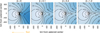 |
Fig. 8 Number density distribution in the PSE equatorial plane near Phaethon on February 22, 2025. In each case, the asteroid ejects the same number of dust particles, all of which are considered to have the same β. |
4 Applications
4.1 3200 Phaethon
Classified as a near-Earth asteroid of the Apollo type, 3200 Phaethon follows a highly eccentric orbit (a = 1.27 AU, e = 0.89, i = 22°), frequently crossing Earth’s orbital path. This object, discovered in 1983 (Green et al. 1985), displays comet-like characteristics and is associated with the annual Geminid meteor shower (Whipple 1983). Remarkably, the impact ejecta production observed from Phaethon along its highly eccentric orbit exceeds that of asteroids in more circular orbits, but it remains minimal compared to the Geminids (Szalay & Horányi 2016b; Szalay et al. 2019). A comparison of the evolution of the Geminid stream and its currently observed stream location near the Sun found that the Geminids were likely created in a catastrophic event (Cukier & Szalay 2023).
In what follows we apply the model developed in the previous sections to calculate the number density of dust (created by impacts of interplanetary grains on the asteroid surface) in the vicinity of Phaethon including the effect of solar radiation pressure. We use the orbital phase at which Phaethon will be visited by the upcoming DESTINY+ JAXA’s mission (Arai et al 2018; Ozaki et al. 2022). We define the distributions of dust ejection speed and direction by applying the results of Szalay et al (2019). In that study, the impact ejecta number density distribution over Phaethon’s surface was inferred (see Fig. 10 of Szalay et al. 2019) from the meteoroid environment in the inner solar system (Nesvorný et al. 2010; Nesvorný et al. 2011a,b; Pokorný et al. 2014) taking into account variations in projectile flux over Phaethon’s orbital period.
4.1.1 Phaethon as a point-like dust source
At first, we neglected the size of Phaethon and evaluated its dust environment modeling dust ejection from a moving point-like object. We used the simple expansion method as the orbital parameters of Phaethon allow for it (see discussion of the simple expansion method applicability in Sects. 2.6 and 3.2). For each model source active at time Tj we employed an impact ejecta map obtained by Szalay et al. (2019) for the given time (or interpolated for the time Tj from the maps obtained for nearby times) to define the distribution of the ejection direction. Each map is a matrix in which for the given grid of latitudes and longitudes, the number density of impact ejecta at the asteroid surface is provided. For any given direction of dust ejection ![$\[(\psi^{\tilde{A}}, \lambda_{M}^{\tilde{A}})\]$](/articles/aa/full_html/2025/01/aa52162-24/aa52162-24-eq54.png) we interpolated from the matrix the corresponding number density, which was then normalized so that the integral of
we interpolated from the matrix the corresponding number density, which was then normalized so that the integral of ![$\[f_{\psi^{\tilde{A}}, \lambda_{M}^{\tilde{A}}}(\psi^{\tilde{A}}, \lambda_{M}^{\tilde{A}})\]$](/articles/aa/full_html/2025/01/aa52162-24/aa52162-24-eq55.png) over the sphere is equal to 1. At the same time, the total number of particles ejected by each source Γ was obtained from the same map by converting number density to the ejecta flux and then integrating over the surface of the spherical asteroid and multiplying by (Tj+1 − Tj). We employed for the ejection speed distribution, the expression determined in Szalay & Horányi (2016a) for Lunar impact ejecta
over the sphere is equal to 1. At the same time, the total number of particles ejected by each source Γ was obtained from the same map by converting number density to the ejecta flux and then integrating over the surface of the spherical asteroid and multiplying by (Tj+1 − Tj). We employed for the ejection speed distribution, the expression determined in Szalay & Horányi (2016a) for Lunar impact ejecta
![$\[f_{u}(u)=\frac{2 h u}{l u_{e}^{2}\left(1-\left(u / u_{e}\right)^{2}\right)^{2}} e^{-\frac{h}{\left.l\left((u /u_{e}\right)^{-2}-1\right)}},\]$](/articles/aa/full_html/2025/01/aa52162-24/aa52162-24-eq56.png) (20)
(20)
with h = 1737 m, ue = 2400 m/s, and l = 200 m, which was also adopted by Szalay et al. (2019) for Phaethon’s impact ejecta.
We determined the dust number density in the vicinity of Phaethon on February 22, 2025 for a dense grid of β values. For each β, we modeled the dust ejection from Phaethon by setting (Tj+1 − Tj) to 60 seconds and took into account the dust ejected for 140 hours before tnow. These parameters were empirically shown to be sufficient for the desired resolution and accuracy of number density. Figure 8 displays the results obtained with the simple expansion method in the Phaethoncentric Solar Ecliptic (PSE) coordinate system, as utilized by Szalay et al. (2019). In the PSE frame, the xy-plane encompasses the center of Phaethon, with the x-axis oriented toward the Sun and z-axis co-directed with the component of ECLIPJ2000 polar axis that is normal to the Phaethon-Sun direction. In Fig. 8 we show results for grains of different values of β, which allows us to compare the respective dust cloud configurations. The distribution of number density depicted in the leftmost image of Fig. 8 (corresponding to β = 0) matches the lower panel of Figure 6 in Szalay et al. (2019), which was derived from a different model approach that ignored the effect of radiation pressure but that employed the same map for the ejecta flux over the asteroid surface. This case (β = 0) develops a higher dust density on the solar facing side of the asteroid, as a result of the large inbound radial velocity component of the asteroid in this time that establishes a high relative velocity to the helion projectile population (Szalay et al. 2019). For β > 0 dust is pushed toward the anti-solar side relative to the asteroid. This leads to an enhancement of the dust number density on the anti-solar side, and the asteroid begins to develop a tail. On the sub-solar side, the changes due to the radiation pressure effect are small relative to the case of β = 0.
In the next step, we calculated the total number density of dust particles within a specified radius range taking into account a plausible relation between β and particle size derived for forsterite, as a prototype astrophysical silicate. These β values are derived with Mie theory (Mie 1908; Bohren & Huffman 1983) from the complex refractive indices of nonporous forsterite (ρ = 3270 kg/m3), measured in laboratory experiments (Suto et al. 2006; Pitman et al. 2013), averaging over the solar spectrum (Mukai 1989). Figure 9 illustrates this relation. Following Szalay & Horányi (2016b) and Szalay et al. (2019) we adopted a power-law differential distribution of particle radii derived from measurements of LDEX at the Moon by (Horányi et al. 2015)
![$\[f_{R}(R)=\frac{1-k}{R_{max}^{1-k}-R_{min}^{1-k}} R^{-k},\]$](/articles/aa/full_html/2025/01/aa52162-24/aa52162-24-eq57.png) (21)
(21)
with k = 3.7, the maximum radius Rmax = 100 μm, and a minimum particle radius Rmin = 0.05 μm, which is a rough estimate of the DESTINY + Dust Analyser (DDA) sensitivity threshold for its flyby of Phaethon. We integrated results for various β(R) over the size distribution defined by Eq. (21). The maximum β value of 0.73 corresponds to R = 0.2 μm. The number density distribution obtained upon this integration is shown in Fig. 102. Due to the steep size distribution, the environment is predominantly populated by dust grains with radii below 0.1 μm, corresponding to β values of about 0.4 to 0.6.
We also derived the number density profile expected for a spacecraft on a circular trajectory. For a direct comparison to Szalay et al. (2019) we present here calculations corresponding to a flyby on February 22, 2025, though the actual DESTINY+ flyby will occur later. Nevertheless, the orbital configuration, and thus the impact ejecta distribution over the asteroid’s surface, will be very close to the case we considered. We assumed that the trajectory lies in the PSE xy-plane and crosses the x-axis of the PSE frame at an angle of 29°. The distance of closest approach to Phaethon is 500 km, as planned for DESTINY+. The dashed line in Fig. 10 corresponds to this trajectory. For comparison, we also evaluated the number density along a trajectory at the same distance from Phaethon but on its anti-solar side. Despite the significant redistribution of dust in the cloud due to radiation pressure, the sub-solar trajectory still passes through a denser region than the anti-solar one because of the abundant ejection of dust on the side facing the Sun. Figure 11 shows the profiles of number density for different size thresholds Rth. Knowing that the effective sensitive area of the DDA is 0.03 m2 (Simolka et al. 2024), we evaluated the cumulative number of dust impacts of particles with R > Rth onto the DDA target during the flybys along the lines in Fig. 10. In case of Rth = 0.1 μm, this number is nearly 3 for the sub-solar trajectory (dashed line), while for the anti-solar flyby (dotted line), it is only 1. For Rth = 0.05 μm, the expected cumulative number of impacts in case of the sub-solar flyby is 19, and for Rth = 0.2 μm the number is 0.3. For comparison, if the same amount of dust were ejected isotropically by Phaethon, the expected number of impacts of particles with R > 0.5 μm would be 1 for any flyby at a distance of 500 km.
The impact velocities of the dust grains on the detector are roughly equal to the spacecraft’s relative velocity to the asteroid. The particles’ velocities relative to the asteroid are at least an order of magnitude smaller than the flyby velocity and can thus be neglected. However, in a rendezvous mission, when the spacecraft’s velocity relative to the asteroid is low, the grains’ peculiar velocities become significant and must be included in the kinetic integral to estimate the dust flux along the spacecraft trajectory.
The dust environment in the close vicinity of the dust source is dominated by particles that have been ejected recently, as the prime clouds with small Δt values are denser (see Fig. 4). Therefore, the spatial distribution of dust is highly sensitive to the shape of the ejection velocity distribution, particularly within the range of relatively small velocities. The distribution obtained by Szalay & Horányi (2016a) from LDEX measurements shows a peak at approximately 600 m/s. To illustrate the effect of varying the ejection velocity distribution on the dust concentration, we evaluate the dust number density around Phaethon employing two distributions that peak at smaller velocities (they are plotted in Fig. 12 and correspond to setting in Eq. (20) l = 1 m and l = 40 m), and a power-law differential distribution with an exponent of −2, representing an extreme case of the peak of the distribution being shifted toward low ejection speeds. All distributions are considered over the interval between umin = 2 m/s (escape velocity of Phaethon) and umax = 2400 m/s (the upper limit of the distribution defined in Szalay & Horányi 2016a). Figure 13 demonstrates how the spatial distribution of dust responds to these changes of the ejection speed distribution. As the peak shifts to smaller values of u, the ejected dust remains more concentrated near the source. Only in the case of the power-law distribution, the radiation pressure acceleration of the dust away from the Sun overcomes the effect of the initial velocity component of grains launched from the sub-solar side directed toward the Sun, resulting in a cloud that is denser on the anti-solar side of the asteroid.
The ejection velocity distribution of impact ejecta depends on the properties of the target surface (see for example Michikami et al. 2007), which may differ significantly in the case of Phaethon compared to the lunar surface. In our modeling, we also neglected a potential dependence of ejection velocity on grain size, which is expected in various physical processes. The data obtained during the DESTINY+ flyby can be used, among other applications, to better constrain the distribution of ejection velocities.
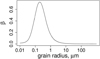 |
Fig. 9 Dependence of β on particle radius for forsterite dust grains. |
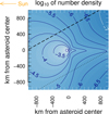 |
Fig. 10 Number density of dust with radii in the range 0.1–100 μm integrated over the differential power-law size distribution with an exponent −3.7. The number density is shown in the PSE equatorial plane near Phaethon on February 22, 2025. Radiation pressure is taken into account. The dashed line shows the trajectory of a flyby that mimics the future DESTINY+ flyby. The dotted line represents the trajectory of a flyby at the same distance from the asteroid, but on the opposite side. |
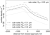 |
Fig. 11 Number density profiles of the flybys along the trajectories shown in Fig. 10 evaluated for three size thresholds Rth = 0.05 μm, Rth = 0.1 μm, and Rth = 0.2 μm. |
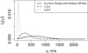 |
Fig. 12 Test distributions of ejection velocity compared to the distribution obtained by Szalay & Horányi (2016a) and employed by Szalay & Horányi (2016b) and Szalay et al. (2019). The distribution fu1(u) corresponds to setting l = 40 m in Eq. (20). The curve fu2(u) is obtained by setting l = 1 m. |
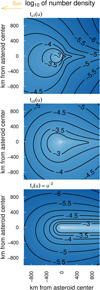 |
Fig. 13 Variations in dust configuration in the close vicinity of Phaethon with changes in the ejection velocity distribution. The number density is computed for particles with radii larger than 0.1 μm. All three distributions of the ejection speed u are normalized over the interval (2, 2400) m/s. The distributions fu1(u) and fu2(u) are shown in Fig. 12. |
 |
Fig. 14 Number density distribution in the PSE equatorial plane near Phaethon on February 22, 2025. Re-collisions of dust grains with Phaethon are taken into account. Phaethon is considered a sphere of radius 2.9 km. Radiation pressure is neglected in the shadow of the asteroid. |
4.1.2 Phaethon as a spherical source of dust
In order to investigate the principal effect of the finite asteroid size on the dust environment we modeled Phaethon as a sphere with a radius of 2.9 km. In this case, we utilized the impact ejecta maps obtained by Szalay et al. (2019) to assign a production rate to each source on the asteroid’s surface based on the source position. The distribution of ejection directions employed in this scenario is uniform, with particles ejected into a cone with an opening angle of 60°, uniformly distributed around the local normal to the asteroid’s surface. The result is obtained for a time interval between the times of dust ejection Tj+1 − Tj = 60 s, with 600 point sources randomly and uniformly distributed over the sphere ejected dust simultaneously. Thus, each source represents dust ejection from a region of approximately 1.8 × 10⁵ m2 area. A new set of random point sources was generated for each time Tj and each particle size, which helped reducing random fluctuations when co-adding contributions from different Tj and averaging over the size distribution. However, small oscillations are still visible in the resulting number density distribution (see Fig. 14).
Figure 14 displays the distribution of dust number density close to the asteroid in the PSE equatorial plane. The region where the number density is depleted due to particles re-impacting the asteroid is narrow. We considered the region directly behind the asteroid being shadowed from sunlight and switched off radiation pressure entirely when calculating the number density in this area. This is a reasonable approximation for the close vicinity of the asteroid and short time intervals since ejection. However, when performing calculations for larger Δt, it is important to note that particles may temporarily enter the asteroid’s shadow and later contribute to the number density outside of the shadow or particles enter the shadow after having followed a path that was influenced by radiation pressure. Mathematically, this means that the value of μR changes over time. DUDI-heliocentric is not capable of resolving such cases. Therefore, the user must choose the most appropriate value of μR as an approximation. For the situation shown in Fig. 14 we used μR = GMS un (i.e., β = 0) for the evaluation of number density in the shadow region.
The asteroid’s shadow in the dust cloud would be crossed within seconds or less by a spacecraft traveling at typical flyby velocity (few to a few 10s of km/s). However, the effect of the shadow may be important for missions that encounter asteroids and comets at low relative speed, like quasi-orbiter missions or sample return missions.
4.2 Comet Hyakutake: SOHO near perihelion observations
In the following example, our objective was not to obtain scientifically valuable results on a dust-ejecting object but rather to demonstrate the nuances of the v-integration method. We applied this method to reconstruct an image of Comet C/1996 B2 (Hyakutake), achieving a general resemblance of the model image to the observed one. Comet Hyakutake, one of the great comets of the twentieth century, was observed near the Sun by the Solar and Heliospheric Observatory (SOHO). The image, shown in Figure 15, was captured by the C3 subsystem of SOHO’s Large Angle Spectroscopic Coronagraph (LASCO) soon after the comet had passed its perihelion.
We neglected the comet’s dimensions and modeled the dust ejection at each point with a single point source. We also disregarded possible temporal changes in the dust ejection rate and the distributions of dust particle sizes, ejection speed, and direction. For the ejection speed distribution, we adopted the normal distribution
![$\[f_{u}(u)=\frac{1}{\sigma \sqrt{2 \pi}} e^{-\frac{\left(u-u_{0}\right)^{2}}{2 \sigma^{2}}},\]$](/articles/aa/full_html/2025/01/aa52162-24/aa52162-24-eq58.png) (22)
(22)
with σ = 50 m/s and u0 = 600R−1/2 m/s, where particle radius R is in microns. Here u0 is the terminal velocity to which particles of size R tend to be accelerated to by the gas outflow (for typical velocities inferred for Hyakutake see Fulle et al. 1997). We modeled the dust emission as a uniform ejection from the sub-solar hemisphere of the comet. The dust production rate of the particles in the considered size range was set to 1020 s−1.
We considered the comet tail to be optically thin based on the estimates of the dust production rate and size distribution by Fulle et al. (1997) inferred from the observations preceding the perihelion passage. We calculated the geometrical optical depth, which is correlated to the brightness of the tail, for a uniform grid of 20 particle radii Ri in the range of (0.2 μm, 2 μm) and the corresponding values of β(Ri). We adopted the relation β(R) for fresh cometary material given by Wilck & Mann (1996) to test our model across a broad range of β values (see also Mann et al. 2004; Kolokolova et al. 2007, for more recent results regarding the subject). The adopted relation has a peak value of β near 0.1 μm particles (see Fig. 2 in Wilck & Mann 1996). The chosen interval of R corresponds to β values between 0.27 and 1.60. The value of Ri = 0.36 μm corresponds to β = 0.997, which is sufficiently far from the critical value β = 1, for which the v-integration method cannot obtain a solution (see Sect. 3.2). If β had been closer to 1, we would have had to adjust the grid of particle radii Ri.
We considered dust ejection for two weeks before the time tnow, for which we construct the image. The model sources were placed along the comet’s trajectory in such a way that they were denser close to tnow, with the interval (Tj+1 − Tj) being as small as 0.5 minutes for dust ejected 5 days before tnow or later. For dust ejected between 10 and 5 days before tnow, the interval (Tj+1 − Tj) was set to 1 minute, and for dust ejected earlier, this interval was 3 minutes. The number of particles ejected by each model source Γ was adjusted accordingly to maintain a constant production rate over the two weeks of dust ejection. The decision to reduce time resolution for earlier dust ejection was based on the fact that the density in prime clouds decreases with time as the prime clouds expand (see Fig. 4), and their relative contribution to the result becomes smaller.
We computed the number density of dust for each β in planes parallel to LASCO’s field of view, cutting the comet’s tail at different distances from the comet’s nucleus. These parallel planes are spaced 5 × 10⁻⁴ AU apart, which provides sufficient resolution for our purpose. The furthest plane we considered in our calculations is located at 0.05 AU from the comet center. Prime clouds with larger corresponding values of β move away from the comet faster than those with smaller β values (see Fig. 3). Therefore, within two weeks before tnow, the furthest plane is reached only by the dust having β > 1.1.
The SOHO image from Fig. 15 was taken shortly after comet Hyakutake had passed its perihelion. To apply our model to this situation we had to utilize the v-integration method’s ability to solve the dynamical problem when dust particles pass their pericenter on the way from the source to the point of interest. In such cases, for every point of interest, the code must be run twice: once with the assumption that the particles passed their perihelion, and another time with the assumption that they did not (see README file in the GitHub repository with the code for a precise instruction on how to set this assumption in the code). In practice, one can integrate the trajectory of the prime cloud center to determine if it has a nonzero density at the point of interest or if the dust grains passed perihelion on their way to it. However, there are limit cases where one prime cloud may be divided into two parts: one part containing particles that have already passed their perihelion and the other composed of particles that did not. Running the code with the assumption that the perihelion passage took place results in zero number density at points where the particles having not yet passed their perihelion would be, and vice versa, as shown in Fig. 16. The lack of connection between the parts is an artifact resulting from the numerical difficulty arising when the dust grains are ejected very close to their perihelion (see Sect. 3.2 for details). The actual dust number density in this region can be recovered via interpolation within the prime cloud. Another possible way to address this is by increasing the time resolution (i.e., the number of model sources used per orbital arc). The prime clouds ejected by different model sources experience numerical problems in different regions. Hence, for every point of interest, we can exclude the prime clouds with singularities and interpolate between those prime clouds whose input to the number density at the given point is computed normally.
We display the results of our modelling as a reconstructed image in terms of the geometric optical depth that is derived for the viewing geometry of the SOHO image shown in Fig. 15. We co-add contributions from different particle sizes (that include the effect of β(R)) with a proper integration over the initial size distribution
![$\[f_{R}(R)=\frac{1-k}{R_{max}^{1-k}-R_{min}^{1-k}} R^{-k}, ~k=4.0.\]$](/articles/aa/full_html/2025/01/aa52162-24/aa52162-24-eq59.png) (23)
(23)
Specifically, for a parallel bundle of straight lines (corresponding to the lines of sight for each pixel in our reconstructed image) we determine the column number density Ni(Ri) for the contribution from each particle size. Then the geometric optical depth for a given pixel is obtained as
![$\[M=\pi \sum_{i=1}^{20} N_{i} f_{R}(R_{i}) R_{i}^{2} \Delta R_{i}.\]$](/articles/aa/full_html/2025/01/aa52162-24/aa52162-24-eq60.png) (24)
(24)
Figure 17 shows the comparison of the model image to the image taken by SOHO/LASCO. We restricted analysis to a visual comparison to demonstrate the principal applicability of DUDI-heliocentric. Our simplified approach could not reproduce the double structure of the comet dust tail visible in the SOHO image, and the ion tail is out of the scope of DUDI-heliocentric. The greater relative brightness near the comet’s nucleus in the observed image may indicate the presence of dust with a smaller β parameter that moves away from the comet’s nucleus more slowly. Dust production rate increasing with time could also lead to a relatively denser region near the nucleus. A wider spread of dust in the SOHO image compared to the model image, in its turn, may be interpreted as a sign of higher ejection speeds of the particles. Nevertheless, the comet tail position and shape in the model image matches the observed one. It shows that the model is capable to reproduce the cometary dust tail structure when compared to images. Combining the analysis with a model for light scattering it will be possible to constrain the size distribution and ejection velocity distribution of the dust in comparison to images of different wavelength and phase angle.
 |
Fig. 15 Comet C/1996 B2 (Hyakutake) observed by the SOHO/LASCO coronagraph C3. The image is taken from the gallery “Best of SOHO.” The date and time of the observation are given in the bottom left corner (May 2, 1996, 23:51 UTC). The field of view of the C3 coronagraph is 15.93° × 15.93°. The square restricts the area with the comet image, which we reconstructed using DUDI-heliocentric. |
 |
Fig. 16 Section of one prime cloud containing dust particles ejected both before and after their perihelion. The resolution is 20 times that used to construct the model image of the comet C/1996 B2 (Hyakutake) in Fig. 17. The mismatch is the result of the singularity appearing in Eq. (9) when a particle is ejected close to the pericenter of its orbit, and so ψ ≈ 90°. |
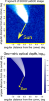 |
Fig. 17 Comparison of the SOHO/LASCO image of the comet Hyakutake and the image constructed with DUDI-heliocentric. |
5 Summary and discussion
In a recent paper (Ershova & Schmidt 2021) we developed a mathematical model for the distribution of dust particles that are ejected from point sources on the surface of a gravitating atmosphereless body, building on previous work by Krivov et al. (2003) and Sremčević et al. (2003). In the present paper we extended this approach to model the ejection of dust from interplanetary sources of dust (e.g., asteroids and comets). The dust can be mobilized for instance by outgassing activity or impacts of interplanetary meteoroids, while for active asteroids a number of additional processes have been discussed (Jewitt 2012). In order to apply the model from Ershova & Schmidt (2021), which is based on the theoretical framework of the gravitational two-body problem, we used the Sun as the central gravitating body and neglected the gravity of the dust source itself. For most applications this is an excellent approximation. Moreover, the approach permits the inclusion of the effect of solar radiation pressure by a renormalization of the solar mass. The dust emission from the source body is described in terms of point sources located on a hypothetical spherical surface with the Sun at its center and a radius that corresponds to the heliocentric distance of the location of the source. The continuous production of dust is approximated by an appropriate number of discrete sources placed along the path of the dust source that remain active for a short period of time. For some applications it is sufficient to approximate the source body as one single dust source, where a non-uniform directional distribution can be taken into account that may have been induced by the directionality of the impactor flux or, in case of cometary activity, the direction of solar insolation. However, it is also possible to account for the finite size of the source body directly, using a (potentially large) number of sources placed appropriately on the surface of the body.
We developed and described three specific methods of solution to the problem. The methods differ in mathematical and numerical complexity as well as their range of applicability to model dust emission from interplanetary sources. One of the methods even allows us to consider forces other than solar gravity and radiation pressure, though only in limited cases.
The v-integration method takes into account only solar gravity and radiation pressure. This method can be applied to the dynamics of dust ejected as long ago as half of the asteroid’s orbital period. It can calculate the number density of dust particles that passed the pericenters of their orbits between the ejection and the time for which the number density is computed. This method allows for the consideration of dust grain re-impacts on the asteroid, but it requires representing the asteroid at each time when it ejects dust not just with one model point source, but hundreds of point sources (the number depends on the asteroid’s size), resulting in a proportional increase in computational workload. This method is suitable for modeling dust ejection in proximity to the Sun and for investigating dust tails far from their sources.
The δ-ejection method uses simplified two-body equations to describe the dynamics of dust under solar gravity and radiation pressure, neglecting other forces. This method can be used to determine the number density of dust ejected from an asteroid along a curved arc of its orbit, though there are limitations to its applicability related to the asteroid’s orbital parameters (see Sect. 3). Re-impacts of the dust with the asteroid can be accounted for if at each point on the asteroid trajectory the asteroid is represented by many sources distributed over its surface. The δ-ejection solution should be selected if one is interested in the number density of dust in the close vicinity of the asteroid, where recently ejected dust dominates the environment, but where the curvature of the asteroid’s trajectory, as well as its physical size or shape, cannot be neglected.
The simple expansion method can be applied when the trajectory of the asteroid can be locally well approximated by a straight line. This method is suitable to evaluate the dust number density in the close vicinity of an asteroid (so that dust ejected recently dominates the environment) being far from its pericenter (so that the curvature of the asteroid trajectory is small). The main assumption of the simple expansion solution is that all forces acting on the dust grains can be regarded as constant within the vicinity of the asteroid. This method allows the effect of various perturbations experienced by the dust cloud to be taken into account, for example the Lorentz force acting on charged particles in the interplanetary magnetic field; however, the re-impacts of the dust particles on their parent body are not considered. The solution is computationally inexpensive, even though separate integration of the trajectory of the prime cloud center is necessary. In DUDI-heliocentric, when using the simple expansion solution method, the coordinates of the prime cloud center are treated as an input parameter.
We applied our model to investigate the dust environment of NEA 3200 Phaethon during the orbital phase at which it will be closely observed by the upcoming DESTINY+ mission by JAXA. During this phase, as Phaethon moves toward the Sun, the majority of dust grains are ejected from the sub-solar hemisphere of the asteroid due to the significantly increased projectile flux from this direction, a result of Phaethon’s motion on its eccentric orbit. We found that radiation pressure significantly redistributes the ejecta toward the anti-solar region because the dust ejected toward the Sun is pushed in the opposite direction by radiation pressure. Within thousands of kilometers from the asteroid, the dust number density is still higher on the sub-solar side than on the anti-solar side as the separation of the dust cloud from the asteroid is slow at 1 AU heliocentric distance. However, on the sub-solar side, there is a limiting distance that the dust can reach due to the influence of radiation pressure, while on the anti-solar side, the dust tail length is limited only by the orbital parameters of the asteroid. We note that an asteroid moving away from the Sun would experience an enhanced projectile flux from the anti-solar direction, resulting in more dust being ejected in the same direction that radiation pressure pushes it. This makes flybys in the anti-solar region highly preferable for dust sampling from bodies on outbound orbits compared to sub-solar flybys.
We found that the spatial configuration of dust number density in the close vicinity of the asteroid is particularly sensitive to the distribution of dust ejection speeds, especially in the range of low velocities. This sensitivity arises because the environment is dominated by recently ejected dust. For Phaethon at the considered orbital phase, an enhanced density in the sub-solar region is observed in the model for a range of choices for the ejection speed distributions (see Fig. 13). However, as the peak of the ejection speed distribution shifts toward lower velocities, the center of mass of the surrounding dust cloud shifts away from the Sun.
We also considered a scenario where the physical size of the asteroid was taken into account, assuming a spherical shape. We evaluated the effect of grain absorption by re-impacts of dust particles on the asteroid. The results show a significant drop in number density, but only within a very narrow region directly behind the asteroid along its heliocentric position vector. This trace is negligible for typical flybys, but could be important for rendezvous missions. Additionally, when a significant number of particles are ejected with a speed distribution that peaks at low velocities, re-impacts can remove a substantial portion of the ejecta from the dust tail and the more massive grains can be expected to have lower ejection speeds. This could result in a depletion of these large particles in Phaethon’s dust tail compared to the initial size distribution of the ejecta.
Finally, we provided a technical example of the application of the v-integration method by reconstructing a SOHO/LASCO image of comet C/1996 B2 (Hyakutake). We outlined the necessary steps and discussed in detail the treatment of dust ejection near the comet’s perihelion.
Our model is implemented as a Fortran-95 software package named DUDI-heliocentric. The code is efficient and easily parallelizable using the OpenMP library. It allows the investigation of a variety of physical problems, even on a personal computer, without the need for large computing clusters. For example, we did not require special computational facilities for the case discussed in Sects. 4.1.1 and 4.2, while a computer cluster of 12 cores was utilized for the calculations in Sect. 4.1.2. DUDI-heliocentric can be applied to model complex dust ejection scenarios, such as those involving collimated jets or catastrophic events where dust ejection changes drastically over time, as well as a stationary or slowly changing ejection from moving objects. The package can also be used to analyze the often complex topology of dust clouds ejected by comets and asteroids (Jewitt et al. 2015) and to relate the topology to the sources and mechanisms of ejection.
Data availability
DUDI-heliocentric is publicly available at https://github.com/Veyza/dudi-heliocentric under the GNU General Public License.
Acknowledgements
This work was supported by the Academy of Finland (AE and JSc). Xiaodong Liu was supported by the National Natural Science Foundation of China (No. 12472048).
Appendix A Jacobian of transformation from the asteroid-centered to heliocentric coordinate system
Ershova & Schmidt (2021) derived a Jacobian for modeling dust ejection into a tilted jet (Eq. (12) of Ershova & Schmidt (2021)). It corresponds to the Jacobian for the transformation from the system A to the system ![$\[\tilde{A}\]$](/articles/aa/full_html/2025/01/aa52162-24/aa52162-24-eq61.png) , both of which are asteroid-centered (see Fig. 5 in the main text). This Jacobian, denoted Jtilt, reads
, both of which are asteroid-centered (see Fig. 5 in the main text). This Jacobian, denoted Jtilt, reads
![$\[\begin{aligned}& J_{tilt}=\left|\frac{\partial(\psi^{\tilde{A}}, \lambda_M^{\tilde{A}})}{\partial(\psi^A, \lambda_M^A)}\right|=4 ~\sin~ \psi^A \times \\& \times[10-2 ~\cos~ 2 \psi^A-3 ~\cos~ 2(\psi^A-\zeta)\\& -2 ~\cos~ 2 \zeta-3 ~\cos~ 2(\psi^A+\zeta) \\& -8 ~\cos~ 2(\lambda_M^A-\eta) ~\sin~ ^2 \zeta ~\sin~ ^2 \psi^A \\& -8 ~\cos~ (\lambda_M^A-\eta) ~\sin~ 2 \zeta ~\sin~ 2 \psi^A]^{-1 / 2},\end{aligned}\]$](/articles/aa/full_html/2025/01/aa52162-24/aa52162-24-eq62.png) (A.1)
(A.1)
where ζ and η are, respectively, the zenith angle and azimuth of the ejection symmetry axis.
In the case of dust ejection by a moving object we must calculate an additional Jacobian Jmotion to perform the variable transformation from the system ![$\[\tilde{S}\]$](/articles/aa/full_html/2025/01/aa52162-24/aa52162-24-eq63.png) to the system A moving relative to the system
to the system A moving relative to the system ![$\[\tilde{S}\]$](/articles/aa/full_html/2025/01/aa52162-24/aa52162-24-eq64.png) with the source velocity V.
with the source velocity V.
The coordinates u, ψ, λM are defined in the system ![$\[\tilde{S}\]$](/articles/aa/full_html/2025/01/aa52162-24/aa52162-24-eq65.png) in Fig. 5. Then the Cartesian coordinates of the vector uA in system A can be expressed as
in Fig. 5. Then the Cartesian coordinates of the vector uA in system A can be expressed as
![$\[\begin{aligned}u_X^A & =u^A ~\sin~ \psi^A ~\cos~ \lambda_M^A \\& =u ~\sin~ \psi ~\cos~ \lambda_M-V_x, \\u_Y^A & =u^A ~\sin~ \psi^A ~\sin~ \lambda_M^A \\& =u ~\sin~ \psi ~\sin~ \lambda_M-V_y, \\u_Z^A & =u^A ~\cos~ \psi^A \\& =u ~\cos~ \psi-V_z,\end{aligned}\]$](/articles/aa/full_html/2025/01/aa52162-24/aa52162-24-eq66.png) (A.2)
(A.2)
where Vx, Vy, Vz are the Cartesian components of the vector V in the system ![$\[\tilde{S}\]$](/articles/aa/full_html/2025/01/aa52162-24/aa52162-24-eq67.png) . The ejection velocity vector in polar coordinates
. The ejection velocity vector in polar coordinates ![$\[(u^{A}, \psi^{A}, \lambda_{M}^{A})\]$](/articles/aa/full_html/2025/01/aa52162-24/aa52162-24-eq68.png) in the system A can be expressed in the following way:
in the system A can be expressed in the following way:
![$\[\begin{aligned}u^A \quad & =[u^2+V^2-2 u(V_x ~\sin~ \psi ~\cos~ \lambda_M \\& +V_y ~\sin~ \psi ~\sin~ \lambda_M+V_z ~\cos~ \psi)]^{1 / 2}, \\\psi^A \quad & =\arccos [(u ~\cos~ \psi-V_z) \times \\& \times(u^2+V^2-2 u(V_x ~\sin~ \psi ~\cos~ \lambda_M \\& +V_y ~\sin~ \psi ~\sin~ \lambda_M+V_z ~\cos~ \psi))^{-1 / 2}], \\\lambda_M^A & =\arctan [u ~\sin~ \psi ~\sin~ \lambda_M-V_y \times \\& \times(u ~\sin~ \psi ~\cos~ \lambda_M-V_x)^{-1}].\end{aligned}\]$](/articles/aa/full_html/2025/01/aa52162-24/aa52162-24-eq69.png) (A.3)
(A.3)
The expression for the azimuth ![$\[\lambda_{M}^{A}\]$](/articles/aa/full_html/2025/01/aa52162-24/aa52162-24-eq70.png) may include an additional constant term +π. However, the presence of this term is irrelevant because Eqs. A.3 are differentiated to obtain the Jacobian for the transformation from
may include an additional constant term +π. However, the presence of this term is irrelevant because Eqs. A.3 are differentiated to obtain the Jacobian for the transformation from ![$\[\tilde{S}\]$](/articles/aa/full_html/2025/01/aa52162-24/aa52162-24-eq71.png) to A
to A
![$\[J_{motion}=\left(\frac{u}{u^A}\right)^2 \frac{\sin \psi}{\sin \psi^A}.\]$](/articles/aa/full_html/2025/01/aa52162-24/aa52162-24-eq72.png) (A.4)
(A.4)
Appendix B Derivatives of the dust grain coordinates in its orbital plane
The coefficients of the Taylor expansion for the particle’s coordinates, defined within its orbital plane, are given by
![$\[a_{x}=-\frac{\mu_{R}}{r_{M}^{2}},\]$](/articles/aa/full_html/2025/01/aa52162-24/aa52162-24-eq73.png) (B.1)
(B.1)
![$\[\dot{a}_{x}=\frac{2 \mu_{R} u_{x}}{r_{M}{ }^{3}},\]$](/articles/aa/full_html/2025/01/aa52162-24/aa52162-24-eq74.png) (B.2)
(B.2)
![$\[\ddot{a}_{x}=\frac{\mu_{R}\left(3 r_{M}\left(u_{y}{ }^{2}-2 u_{x}{ }^{2}\right)-2 \mu_{R}\right)}{r_{M}{ }^{5}},\]$](/articles/aa/full_html/2025/01/aa52162-24/aa52162-24-eq75.png) (B.3)
(B.3)
![$\[a_{x}^{(3)}=\frac{2 \mu_{R} u_{x}\left(11 \mu_{R}+6 r_{M}\left(2 u_{x}{ }^{2}-3 u_{y}{ }^{2}\right)\right)}{r_{M}{ }^{6}},\]$](/articles/aa/full_html/2025/01/aa52162-24/aa52162-24-eq76.png) (B.4)
(B.4)
![$\[\begin{aligned}a_x^{(4)}= & \frac{\mu_R}{r_M^8}\left[6 \mu_R r_M(11 u_y{ }^2-34 u_x{ }^2)-22 \mu_R^2\right. \\& \left.-15 r_M{ }^2(8 u_x{ }^4-24 u_x{ }^2 u_y{ }^2+3 u_y{ }^4)\right]\end{aligned}\]$](/articles/aa/full_html/2025/01/aa52162-24/aa52162-24-eq77.png) (B.5)
(B.5)
![$\[\dot{a}_{y}=-\frac{\mu_{R} u_{y}}{r_{M}{ }^{3}},\]$](/articles/aa/full_html/2025/01/aa52162-24/aa52162-24-eq78.png) (B.6)
(B.6)
![$\[\ddot{a}_{y}=\frac{6 \mu_{R} u_{x} u_{y}}{r_{M}{ }^{4}},\]$](/articles/aa/full_html/2025/01/aa52162-24/aa52162-24-eq79.png) (B.7)
(B.7)
![$\[a_{y}^{(3)}=\frac{\mu_{R} u_{y}\left(9 r_{M}\left(u_{y}{ }^{2}-4 u_{x}{ }^{2}\right)-8 \mu_{R}\right)}{r_{M}{ }^{6}},\]$](/articles/aa/full_html/2025/01/aa52162-24/aa52162-24-eq80.png) (B.8)
(B.8)
![$\[a_{y}^{(4)}=\frac{30 \mu_{R} u_{x} u_{y}\left(5 \mu_{R}+8 r_{M} u_{x}{ }^{2}-6 r_{M} u_{y}{ }^{2}\right)}{r_{M}{ }^{7}}.\]$](/articles/aa/full_html/2025/01/aa52162-24/aa52162-24-eq81.png) (B.9)
(B.9)
Thus, Eqs. 13 and 14 read
![$\[\begin{aligned}0 & =-\frac{\Delta t^6 \mu_R u_x{}^4}{6 r_M{ }^6}+\frac{\Delta t{}^5 \mu_R u_x{}^3}{5 r_M{ }^5} \\& +u_x{}^2\left(-\frac{17 \Delta t^6 \mu_R^2}{60 r_M{}^7}+\frac{\Delta t^6 \mu_R u_y{}^2}{2 r_M{ }^6}-\frac{\Delta t^4 \mu_R}{4 r_M{ }^4}\right) \\& +u_x\left(\frac{11 \Delta t^5 \mu_R^2}{60 r_M{ }^6}-\frac{3 \Delta t^5 \mu_R u_y{}^2}{10 r_M{ }^5}+\frac{\Delta t^3 \mu_R}{3 r_M{ }^3}+\Delta t\right) \\& -\frac{\Delta t^4 \mu_R^2}{12 r_M{}^5}+\frac{\Delta t{}^4 \mu_R u_y{}^2}{8 r_M{}^4}-\frac{\Delta t^2 \mu_R}{2 r_M{}^2}-\frac{11 \Delta t^6 \mu_R^3}{360 r_M{}^8} \\& +\frac{11 \Delta t^6 \mu_R^2 u_y{}^2}{120 r_M{}^7}-\frac{\Delta t^6 \mu_R u_y{}^4}{16 r_M^6}+r_M-x,\end{aligned}\]$](/articles/aa/full_html/2025/01/aa52162-24/aa52162-24-eq82.png) (B.10)
(B.10)
![$\[\begin{aligned}0 & =u_y{}^3\left(\frac{3 \Delta t^5 \mu_R}{40 r_M{}^5}-\frac{\Delta t^6 \mu_R u_x}{4 r_M{}^6}\right) \\+ & u_y\left(\frac{5 \Delta t^6 \mu_R^2 u_x}{24 r_M{}^7}+\frac{\Delta t^6 \mu_R u_x{}^3}{3 r_M{}^6}\right. \\& \left.-\frac{\Delta t^5 \mu_R^2}{15 r_M{}^6}-\frac{3 \Delta t^5 \mu_R u_x{}^2}{10 r_M{}^5}+\frac{\Delta t^4 \mu_R u_x}{4 r_M{}^4}-\frac{\Delta t^3 \mu_R}{6 r_M{}^3}+\Delta t\right).\end{aligned}\]$](/articles/aa/full_html/2025/01/aa52162-24/aa52162-24-eq83.png) (B.11)
(B.11)
Appendix C Dust grains re-impacting the asteroid
When a particle is ejected from the side of the asteroid that faces the Sun, radiation pressure pushes it back toward the asteroid, potentially resulting in a re-impact. To influence the resulting number density, the re-impact must occur within the time interval of length Δt from the time of ejection Tj to the time for which we compute number density tnow (see Table 1). The majority of such events happen shortly after ejection. Therefore, in order to take into account the depletion of the dust density due to re-impacts with the parent body we may use a second-order approximation
![$\[\Delta \mathbf{d}=\Delta \mathbf{d}_{0}+\Delta \mathbf{u} t+\frac{\Delta \boldsymbol{a}}{2} t^{2}+\frac{\Delta \dot{\boldsymbol{a}}}{6} t^{3}+\frac{\Delta \ddot{\boldsymbol{a}}}{24} t^{4},\]$](/articles/aa/full_html/2025/01/aa52162-24/aa52162-24-eq84.png) (C.1)
(C.1)
where Δd is the difference of the position vectors of the asteroid center and the particle position at time t since the time of ejection. The symbols Δd0, Δu, and Δa denote, respectively, the differences of the position, velocity and acceleration vectors of the asteroid center and the particle at the time of ejection.
Bearing in mind that in the time of ejection (t = 0) the particle was at distance Δd0 from the asteroid center, we can transform Eq. (C.1) in the following way neglecting terms of higher orders
![$\[\begin{aligned}& \Delta \mathbf{d}^2=\Delta \mathbf{d}_0^2+\Delta \mathbf{u}^2 t^2+\frac{\Delta \boldsymbol{a}^2}{4} t^4+2 \Delta \mathbf{d}_0 \cdot \Delta \mathbf{u} ~t \\&+\Delta \mathbf{d}_0 \cdot \Delta \boldsymbol{a} ~t^2+\Delta \mathbf{u} \cdot \Delta \boldsymbol{a} ~t^3+\frac{\Delta \mathbf{d}_0 \dot{\boldsymbol{a}}}{3} t^3 \\&\qquad\qquad\quad\quad~~+\frac{\Delta \mathbf{u} \Delta \dot{\boldsymbol{a}}}{3} t^4+\frac{\Delta \mathbf{d}_0 \Delta \ddot{\boldsymbol{a}}}{12} t^4,\end{aligned}\]$](/articles/aa/full_html/2025/01/aa52162-24/aa52162-24-eq85.png) (C.2)
(C.2)
such that the time for re-collision ![$\[\left(\Delta d^{2}=\Delta d_{0}^{2}\right)\]$](/articles/aa/full_html/2025/01/aa52162-24/aa52162-24-eq86.png) is given by the cubic equation
is given by the cubic equation
![$\[\begin{aligned}& \left(\frac{\Delta \boldsymbol{a}^2}{4}+\frac{\Delta \mathbf{u} \Delta \dot{\boldsymbol{a}}}{3}+\frac{\Delta \mathbf{d}_0 \Delta \ddot{\boldsymbol{a}}}{12}\right) t^3 \\& +\left(\frac{\Delta \mathbf{d}_0 \dot{\boldsymbol{a}}}{3}+\Delta \mathbf{u} \cdot \Delta \boldsymbol{a}\right) t^2 \\& \qquad+\left(\Delta u^2+\Delta \mathbf{d}_0 \cdot \Delta \boldsymbol{a}\right) t+2 \Delta \mathbf{d}_0 \cdot \Delta \mathbf{u}=0.\end{aligned}\]$](/articles/aa/full_html/2025/01/aa52162-24/aa52162-24-eq87.png) (C.3)
(C.3)
Here the terms ![$\[\Delta \mathbf{u} \Delta \dot{\boldsymbol{a}} / 3\]$](/articles/aa/full_html/2025/01/aa52162-24/aa52162-24-eq88.png) and Δd0Δä/12 are negligible and omitted in the computational algorithm. If Eq. C.3 has a positive real root smaller than Δt, the particle re-collides with the asteroid.
and Δd0Δä/12 are negligible and omitted in the computational algorithm. If Eq. C.3 has a positive real root smaller than Δt, the particle re-collides with the asteroid.
References
- Arai, T., Kobayashi, M., Ishibashi, K., et al. 2018, in 49th Annual Lunar and Planetary Science Conference, Lunar and Planetary Science Conference, 2570 [Google Scholar]
- Battams, K., & Knight, M. M. 2017, Philos. Trans. Roy. Soc. Lond. A, 375, 20160257 [Google Scholar]
- Bohren, C. F., & Huffman, D. R. 1983, Absorption and Scattering of Light by Small Particles (New York: Wiley-Interscience) [Google Scholar]
- Borin, P., Cremonese, G., Marzari, F., & Lucchetti, A. 2017, A&A, 605, A94 [NASA ADS] [CrossRef] [EDP Sciences] [Google Scholar]
- Bradley, J. P. 2003, Treatise Geochem., 1, 711 [NASA ADS] [Google Scholar]
- Burns, J. A., Lamy, P., & Soter, S. 1979, Icarus, 40, 1 [NASA ADS] [CrossRef] [Google Scholar]
- Chambers, J. E. 1999, MNRAS, 304, 793 [Google Scholar]
- Chen, Z., Yang, K., & Liu, X. 2024, MNRAS, 527, 11327 [Google Scholar]
- Crovisier, J., Bockelée-Morvan, D., Colom, P., & Biver, N. 2016, Comptes Rendus Phys., 17, 985 [NASA ADS] [CrossRef] [Google Scholar]
- Cukier, W. Z., & Szalay, J. R. 2023, Planet. Sci. J., 4, 109 [NASA ADS] [CrossRef] [Google Scholar]
- DellaGiustina, D. N., Nolan, M. C., Polit, A. T., et al. 2023, Planet. Sci. J., 4, 198 [CrossRef] [Google Scholar]
- Ershova, A., & Schmidt, J. 2021, A&A, 650, A186 [NASA ADS] [CrossRef] [EDP Sciences] [Google Scholar]
- Finson, M. J., & Probstein, R. F. 1968a, ApJ, 154, 327 [Google Scholar]
- Finson, M. L., & Probstein, R. F. 1968b, ApJ, 154, 353 [NASA ADS] [CrossRef] [Google Scholar]
- Fulle, M., Mikuz, H., & Bosio, S. 1997, A&A, 324, 1197 [NASA ADS] [Google Scholar]
- Green, S. F., Davies, J. K., Eaton, N., Stewart, B. C., & Meadows, A. J. 1985, Icarus, 64, 517 [NASA ADS] [CrossRef] [Google Scholar]
- Horányi, M., Szalay, J. R., Kempf, S., et al. 2015, Nature, 522, 324 [CrossRef] [Google Scholar]
- Hui, M.-T. 2023, RNAAS, 7, 239 [NASA ADS] [Google Scholar]
- Jackson, A. A., & Zook, H. A. 1992, Icarus, 97, 70 [NASA ADS] [CrossRef] [Google Scholar]
- Jewitt, D. 2012, AJ, 143, 66 [CrossRef] [Google Scholar]
- Jewitt, D., Hsieh, H., & Agarwal, J. 2015, in Asteroids IV, 221 [Google Scholar]
- Jo, H., & Ishiguro, M. 2024, A&A, 683, A68 [NASA ADS] [CrossRef] [EDP Sciences] [Google Scholar]
- Knight, M. M., Kokotanekova, R., & Samarasinha, N. H. 2023, arXiv e-prints [arXiv:2304.09309] [Google Scholar]
- Kolokolova, L., Kimura, H., Kiselev, N., & Rosenbush, V. 2007, A&A, 463, 1189 [NASA ADS] [CrossRef] [EDP Sciences] [Google Scholar]
- Krivov, A. V., Sremčević, M., Spahn, F., Dikarev, V., & Kholshevnikov, K. V. 2003, Planet. Space Sci., 51, 251 [NASA ADS] [CrossRef] [Google Scholar]
- Krüger, H., Krivov, A. V., & Grün, E. 2000, Planet. Space Sci., 48, 1457 [CrossRef] [Google Scholar]
- Lauretta, D. S., Balram-Knutson, S. S., Beshore, E., et al. 2017, Space Sci. Rev., 212, 925 [Google Scholar]
- Levison, H. F., Olkin, C. B., Noll, K. S., et al. 2021, Planet. Sci. J., 2, 171 [CrossRef] [Google Scholar]
- Liu, X., & Schmidt, J. 2018, A&A, 609, A57 [NASA ADS] [CrossRef] [EDP Sciences] [Google Scholar]
- Liu, X., & Schmidt, J. 2019, Astrodynamics, 3, 17 [CrossRef] [Google Scholar]
- Liu, X., & Schmidt, J. 2021, MNRAS, 500, 2979 [Google Scholar]
- Liu, X., Sachse, M., Spahn, F., & Schmidt, J. 2016, J. Geophys. Res.-Planet., 121, 1141 [NASA ADS] [CrossRef] [Google Scholar]
- Mann, I., Kimura, H., & Kolokolova, L. 2004, JQSRT, 89, 291 [NASA ADS] [CrossRef] [Google Scholar]
- Marschall, R., Zakharov, V., Tubiana, C., et al. 2022, A&A, 666, A151 [NASA ADS] [CrossRef] [EDP Sciences] [Google Scholar]
- Martin, M. G., Alred, J. M., Hoey, W. A., Ly, C. S., & Soares, C. E. 2022, SPIE Conf. Ser., 12224, 122240J [NASA ADS] [Google Scholar]
- Marzari, F., & Vanzani, V. 1994, A&A, 283, 275 [NASA ADS] [Google Scholar]
- Michikami, T., Moriguchi, K., Hasegawa, S., & Fujiwara, A. 2007, Planet. Space Sci., 55, 70 [CrossRef] [Google Scholar]
- Mie, G. 1908, Ann. Phys., 330, 377 [Google Scholar]
- Morfill, G. E., & Grün, E. 1979, Planet. Space Sci., 27, 1269 [NASA ADS] [CrossRef] [Google Scholar]
- Mukai, T. 1989, in Evolution of Interstellar Dust and Related Topics, eds. A. Bonetti, J. M. Greenberg, & S. Aiello, 397 [Google Scholar]
- Nesvorný, D., Jenniskens, P., Levison, H. F., et al. 2010, ApJ, 713, 816 [CrossRef] [Google Scholar]
- Nesvorný, D., Janches, D., Vokrouhlický, D., et al. 2011a, ApJ, 743, 129 [CrossRef] [Google Scholar]
- Nesvorný, D., Vokrouhlický, D., Pokorný, P., & Janches, D. 2011b, ApJ, 743, 37 [CrossRef] [Google Scholar]
- Ozaki, N., Yamamoto, T., Gonzalez-Franquesa, F., et al. 2022, Acta Astron., 196, 42 [NASA ADS] [CrossRef] [Google Scholar]
- Pitman, K. M., Hofmeister, A. M., & Speck, A. K. 2013, Earth Planets Space, 65, 129 [Google Scholar]
- Pokorný, P., Vokrouhlický, D., Nesvorný, D., Campbell-Brown, M., & Brown, P. 2014, ApJ, 789, 25 [CrossRef] [Google Scholar]
- Postberg, F., Schmidt, J., Hillier, J. K., Kempf, S., & Srama, R. 2011, Nature, 474, 620 [NASA ADS] [CrossRef] [Google Scholar]
- Russell, C. T., & Raymond, C. A. 2011, Space Sci. Rev., 163, 3 [NASA ADS] [CrossRef] [Google Scholar]
- Saito, J., Miyamoto, H., Nakamura, R., et al. 2006, Science, 312, 1341 [NASA ADS] [CrossRef] [Google Scholar]
- Simolka, J., Blanco, R., Ingerl, S., et al. 2024, Phil. Trans. R. Soc. A, 382, 20230199 [Google Scholar]
- Snodgrass, C., & Jones, G. H. 2019, Nat. Commun., 10, 5418 [NASA ADS] [CrossRef] [Google Scholar]
- Sremčević, M., Krivov, A. V., & Spahn, F. 2003, Planet. Space Sci., 51, 455 [CrossRef] [Google Scholar]
- Suto, H., Sogawa, H., Tachibana, S., et al. 2006, MNRAS, 370, 1599 [CrossRef] [Google Scholar]
- Szalay, J. R., & Horányi, M. 2016a, Geophys. Res. Lett., 43, 4893 [NASA ADS] [CrossRef] [Google Scholar]
- Szalay, J. R., & Horányi, M. 2016b, ApJ, 830, L29 [NASA ADS] [CrossRef] [Google Scholar]
- Szalay, J. R., Pokorný, P., Horányi, M., et al. 2019, Planet. Space Sci., 165, 194 [NASA ADS] [CrossRef] [Google Scholar]
- Taylor, M. G. G. T., Altobelli, N., Buratti, B. J., & Choukroun, M. 2017, Philos. Trans. Roy. Soc. Lond. A, 375, 20160262 [NASA ADS] [Google Scholar]
- Veverka, J., Thomas, P., Harch, A., et al. 1997, Science, 278, 2109 [NASA ADS] [CrossRef] [Google Scholar]
- Waszczak, A., Ofek, E. O., Aharonson, O., et al. 2013, MNRAS, 433, 3115 [NASA ADS] [CrossRef] [Google Scholar]
- Watanabe, S.-i., Tsuda, Y., Yoshikawa, M., et al. 2017, Space Sci. Rev., 208, 3 [Google Scholar]
- Whipple, F. L. 1983, IAU Circ., 3881, 1 [NASA ADS] [Google Scholar]
- Wilck, M., & Mann, I. 1996, Planet. Space Sci., 44, 493 [Google Scholar]
- Yang, K., Schmidt, J., Feng, W., & Liu, X. 2022, A&A, 659, A120 [NASA ADS] [CrossRef] [EDP Sciences] [Google Scholar]
- Zhang, T., Xu, K., & Ding, X. 2021, Nat. Astron., 5, 730 [NASA ADS] [CrossRef] [Google Scholar]
Available at https://github.com/Veyza/dudi-heliocentric
The DUDI-heliocentric GitHub repository contains the necessary routines and input files to calculate the number density distribution shown in Fig. 10.
All Tables
All Figures
|
Fig. 1 Geometry of the model studied by Ershova & Schmidt (2021) transferred to the heliocentric coordinate system. The vector v⊥ is the projection of vector v onto the plane tangential to the sphere centered at the Sun and that contains the position of the source on the asteroid, located at position rM. The remaining variables are defined in Table 1. |
| In the text | |
|
Fig. 2 Moving dust source represented by many sources placed along the given trajectory. Each of these sources is active for a short or infinitely small period of time around Tj. |
| In the text | |
|
Fig. 3 Prime dust clouds ejected by a point source at the same time. The direction of the asteroid motion (apex) is shown relative to the direction toward the Sun. The cross sections of number density (m−3) in the orbital plane of the source are shown at 50 minutes after ejection. The black dot indicates the position of the asteroid center at the same time. The total number of dust particles in each prime cloud is the same (105 grains) with fixed grain sizes that correspond in each case to values of the parameter μR of GMS un, 0.4GMS un, −0.2GMS un, which determines the dust dynamics. The centers of these prime clouds lie on a synchrone. |
| In the text | |
|
Fig. 4 Prime dust clouds ejected by a point source at three different times. The direction of the asteroid motion (apex) is shown relative to the direction toward the Sun. Each prime cloud contains 105 dust particles. The cross section of particle number density (m−3) in the orbital plane of the source is shown 30 minutes (left) after ejection, 60 minutes (middle), and 90 minutes (right). The black dot indicates the position of the asteroid 90 minutes after the first prime cloud was ejected. All particles in the three prime clouds are of the same size corresponding to μR = 0.5GMS un. The centers of these prime clouds lie on a syndyne. |
| In the text | |
|
Fig. 5 Position vectors of dust source rM and spacecraft r (in spherical coordinates (rM, αM, ωM) and (r, α, ω), respectively), defined in the Suncentered system S (compare to Fig. 1). The particle velocity vector at the time of ejection (u, ψ, λM) is defined in the coordinate system |
| In the text | |
|
Fig. 6 Comparison of DUDI-heliocentric to results obtained by the direct integration of trajectories. The dust cloud in the left panel, obtained with DUDI-heliocentric, is shown in the plane normal to the asteroid orbital plane and containing the asteroid’s instantaneous heliocentric position vector. The dust was ejected 15 min before tnow from 2000 sources uniformly distributed on the surface of a spherical asteroid with 5 km radius. Radiation pressure is considered, with β set to 0.5, and dust grain re-collisions with the asteroid are taken into account. The lines in the left panel represent the cuts for which number densities are displayed in the right panel. |
| In the text | |
|
Fig. 7 Profiles of the spherically symmetric prime dust cloud ejected by a point source on the orbit of comet C/2011 W3 (Lovejoy) with e = 0.99993. The dust number density is evaluated 20 hours after the ejection. The profile in the upper panel lies in the source’s orbital plane and passes through the cloud center. This center has developed a hollow because of a nonzero minimum ejection velocity umin (see Sect. 2.2). The profile in the lower panel is normal to the source’s orbital plane, piercing this plane at 20 km distance from the cloud center. |
| In the text | |
|
Fig. 8 Number density distribution in the PSE equatorial plane near Phaethon on February 22, 2025. In each case, the asteroid ejects the same number of dust particles, all of which are considered to have the same β. |
| In the text | |
|
Fig. 9 Dependence of β on particle radius for forsterite dust grains. |
| In the text | |
|
Fig. 10 Number density of dust with radii in the range 0.1–100 μm integrated over the differential power-law size distribution with an exponent −3.7. The number density is shown in the PSE equatorial plane near Phaethon on February 22, 2025. Radiation pressure is taken into account. The dashed line shows the trajectory of a flyby that mimics the future DESTINY+ flyby. The dotted line represents the trajectory of a flyby at the same distance from the asteroid, but on the opposite side. |
| In the text | |
|
Fig. 11 Number density profiles of the flybys along the trajectories shown in Fig. 10 evaluated for three size thresholds Rth = 0.05 μm, Rth = 0.1 μm, and Rth = 0.2 μm. |
| In the text | |
|
Fig. 12 Test distributions of ejection velocity compared to the distribution obtained by Szalay & Horányi (2016a) and employed by Szalay & Horányi (2016b) and Szalay et al. (2019). The distribution fu1(u) corresponds to setting l = 40 m in Eq. (20). The curve fu2(u) is obtained by setting l = 1 m. |
| In the text | |
|
Fig. 13 Variations in dust configuration in the close vicinity of Phaethon with changes in the ejection velocity distribution. The number density is computed for particles with radii larger than 0.1 μm. All three distributions of the ejection speed u are normalized over the interval (2, 2400) m/s. The distributions fu1(u) and fu2(u) are shown in Fig. 12. |
| In the text | |
|
Fig. 14 Number density distribution in the PSE equatorial plane near Phaethon on February 22, 2025. Re-collisions of dust grains with Phaethon are taken into account. Phaethon is considered a sphere of radius 2.9 km. Radiation pressure is neglected in the shadow of the asteroid. |
| In the text | |
|
Fig. 15 Comet C/1996 B2 (Hyakutake) observed by the SOHO/LASCO coronagraph C3. The image is taken from the gallery “Best of SOHO.” The date and time of the observation are given in the bottom left corner (May 2, 1996, 23:51 UTC). The field of view of the C3 coronagraph is 15.93° × 15.93°. The square restricts the area with the comet image, which we reconstructed using DUDI-heliocentric. |
| In the text | |
|
Fig. 16 Section of one prime cloud containing dust particles ejected both before and after their perihelion. The resolution is 20 times that used to construct the model image of the comet C/1996 B2 (Hyakutake) in Fig. 17. The mismatch is the result of the singularity appearing in Eq. (9) when a particle is ejected close to the pericenter of its orbit, and so ψ ≈ 90°. |
| In the text | |
|
Fig. 17 Comparison of the SOHO/LASCO image of the comet Hyakutake and the image constructed with DUDI-heliocentric. |
| In the text | |
Current usage metrics show cumulative count of Article Views (full-text article views including HTML views, PDF and ePub downloads, according to the available data) and Abstracts Views on Vision4Press platform.
Data correspond to usage on the plateform after 2015. The current usage metrics is available 48-96 hours after online publication and is updated daily on week days.
Initial download of the metrics may take a while.