| Issue |
A&A
Volume 696, April 2025
|
|
|---|---|---|
| Article Number | L2 | |
| Number of page(s) | 7 | |
| Section | Letters to the Editor | |
| DOI | https://doi.org/10.1051/0004-6361/202452156 | |
| Published online | 28 March 2025 | |
Letter to the Editor
Data-constrained 3D magnetohydrodynamics simulation of a spiral jet caused by an unstable flux rope embedded in a fan–spine configuration
1
School of Astronomy and Space Science, Nanjing University, Nanjing 210046, PR China
2
Key Laboratory of Modern Astronomy and Astrophysics (Nanjing University), Ministry of Education, Nanjing 210093, China
3
Max Planck Institute for Solar System Research, Justus-von-Liebig-Weg 3, 37077 Göttingen, Germany
4
Institut für Sonnenphysik (KIS), Georges-Köhler-Allee 401A, 79110 Freiburg, Germany
5
Centre for Mathematical Plasma Astrophysics, Department of Mathematics, KU Leuven, Celestijnenlaan 200B, B-3001 Leuven, Belgium
6
Institute of Physics, University of Maria Curie-Skłodowska, Pl. Marii Curie-Skłodowskiej 5, 20-031 Lublin, Poland
⋆ Corresponding author; This email address is being protected from spambots. You need JavaScript enabled to view it.
Received:
6
September
2024
Accepted:
13
March
2025
Abstract
Spiral jets are impulsive plasma ejections that typically show an apparent rotational motion. Their generation, however, is still not understood thoroughly. Based on a high-resolution vector magnetogram from the Polarimetric and Helioseismic Imager on board Solar Orbiter, we constructed a data-constrained three-dimensional (3D) magnetohydrodynamics (MHD) model, aiming to disclose the eruption mechanism of a tiny spiral jet at a moss region observed on March 3, 2022. The initial configuration of the simulation consists of an extrapolated coronal magnetic field based on the vector magnetogram and an inserted unstable flux rope constructed by the regularized Biot-Savart laws method. Our results highlight the critical role of the fan-spine configuration in forming the spiral jet, and confirm the collapse of the pre-existing magnetic null to a curved 3D current sheet where external reconnection takes places. It is further disclosed that the flux rope quickly moves upward, reconnecting with the field lines near the outer spine, thereby enabling the transfer of twisting and cool material from the flux rope to the open field, giving rise to the tiny spiral jet we observed. The notable similarities between these characteristics and those for larger-scale jets suggest that spiral jets, regardless of their scale, essentially share the same eruption mechanism.
Key words: magnetic reconnection / magnetohydrodynamics (MHD) / Sun: corona / Sun: magnetic fields
© The Authors 2025
 Open Access article, published by EDP Sciences, under the terms of the Creative Commons Attribution License (https://creativecommons.org/licenses/by/4.0), which permits unrestricted use, distribution, and reproduction in any medium, provided the original work is properly cited.
This article is published in open access under the Subscribe to Open model. This email address is being protected from spambots. You need JavaScript enabled to view it. to support open access publication.
1. Introduction
Coronal jets are transient collimated outflows that appear bright in extreme ultraviolet (EUV; Wang et al. 1998) and soft X-ray (SXR; Shibata et al. 1992) observations. They are of significant interest as they can transfer mass and energy to the outer corona and solar wind (Priest & Syntelis 2021; Shen 2021). Thanks to recent high-resolution observations, coronal jets are even found to share a similar physical origin with large-scale solar eruptions such as coronal mass ejections (Sterling et al. 2015; Liu et al. 2015; Joshi et al. 2020), and may contribute to partial acceleration in solar wind (Moore et al. 2011; Chitta et al. 2023).
Magnetic reconnection, a fundamental process in magnetized plasma that converts magnetic energy to other forms, is assumed to be the key driver of coronal jets. It has been widely studied in observations and theoretical models (Shibata et al. 1992, 2007; Schmieder et al. 2014; Wyper & DeVore 2016; Tian et al. 2018). Variations in the morphology of jets as observed in soft X-ray (SXR) and extreme ultraviolet (EUV) images, along with the inferred sudden changes in magnetic connectivities apparent from the changes in emission patterns, have been extensively used as evidence for reconnection. Innes et al. (1997) reported spectral evidence that shows red and blue shifts in Si IV 1393 Å line profiles, indicating the presence of bidirectional jets ejected from reconnection sites. Additionally, Shimojo & Shibata (2000) reported a SXR jet with a morphology closely related to micro-flares generated by magnetic reconnection.
Inferring magnetic reconnection based solely on observations is not straightforward. Magnetohydrodynamics (MHD) simulations provide a robust approach to exploring the reconnection and the relation to coronal jets. Yokoyama & Shibata (1996) conducted a 2D MHD simulation, demonstrating that jets can be produced when newly emerging magnetic flux reconnects with the oblique background field. Subsequent studies found that 3D reconnection between the twisted core field and ambient open field can generate spiral jets in coronal holes (Pariat et al. 2009, 2010). Recently, Wyper et al. (2019) simulated a spiral jet and found that it is caused by a combination of magnetic breakout and kink instability of the pre-existing flux rope, which is formed through imposing artificial surface motions at the bottom boundary.
Complementary to MHD simulations, observational data-constrained or data-driven simulations have become a promising method for reproducing coronal jets and even more complex events. Cheung et al. (2015) presented time-dependent magneto-frictional data-driven simulations of recurrent jets originating from a fan–spine magnetic system. Nayak et al. (2019) demonstrated the mini-filament breakout model using a 3D data-constrained MHD simulation. This approach also facilitates a more detailed analysis of thermodynamic and topological properties (Guo et al. 2023). Additionally, Jiang et al. (2016) identified the positive feedback between emerging flux and external magnetic reconnection as a crucial factor for the evolution transiting to the eruptive state.
Recently, Cheng et al. (2023) reported a new observation of persistent null-point reconnection in the EUV at the smallest spatial scale (about 390 km) to date, during which an interesting spiral jet was also observed, lasting for 10 minutes and being identified as arising from a mini-filament eruption. Based on EUV images from the High-Resolution Imager (HRIEUV) at 174 Å of the Extreme-Ultraviolet Imager (EUI; Rochus et al. 2020) on board Solar Orbiter (Müller et al. 2020), the jet of interest, originating from the tiny null point configuration, was found to closely resemble typically observed spiral jets (Raouafi et al. 2016), albeit on a smaller scale. To further understand the generation of this tiny spiral jet and unresolved transfer of the mass and twist from the lower atmosphere to the corona in observations, we employed an observational data-constrained simulation using the Message Passing Interface Adaptive Mesh Refinement Versatile Advection Code (MPI-AMRVAC; Keppens et al. 2003, 2012; Xia et al. 2018), the initial condition of which is well constrained by the high-resolution vector magnetogram provided by the Polarimetric and Helioseismic Imager (SO/PHI; Solanki et al. 2020) on board Solar Orbiter. The data and numerical methodology are described in Sect. 2. The numerical results are presented in Sect. 3, followed by a summary and discussions in Sect. 4.
2. Observation and numerical setup
Observations from multiple EUV passbands of the Atmospheric Imaging Assembly (AIA; Lemen et al. 2012) on board the Solar Dynamics Observatory (SDO; Pesnell et al. 2012) have been extensively analyzed by Cheng et al. (2023). Here, we give an overview of this jet event as observed by HRIEUV on board Solar Orbiter. The details of processing the dataset are provided in Appendix A. This tiny spiral jet, arising from a moss region between two active regions, began around 10:11 UT on March 3, 2022, and lasted for approximately 10 minutes, featuring a spiral motion of dark and bright threads. The zoomed-in line-of-sight (LOS) magnetogram reveals that the jet is located above a small positive polarity region embedded within a predominantly negative polarity region (Fig. B.1b). This configuration suggests a fan–spine configuration, where the spine connects the inner positive polarity enclosed by the fan, with footpoints rooted in surrounding negative polarities, as confirmed in Cheng et al. (2023). This configuration remained relatively unchanged throughout the process despite some disturbances. Figures 1a1–a3 shows the evolution of the spiral jet. As suggested by Cheng et al. (2023), the magnetic reconnection continuously occurred at the null point before the jet, rendering a faint jet spire visible before the eruption. During the eruption, the mini-filament (threaded by a sheared magnetic field; e.g., Sterling et al. 2015) began to ascend rapidly, resulting in a spiral jet characterized by fragmented cool plasma ejecting and propagating along the outer spire toward the farther end.
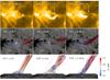 |
Fig. 1. Comparison between observations and simulations at three instances. (a) EUI 174 Å images displaying the temporal evolution of the spiral jet eruption with arrows indicating dark threads. The blue dashed curve in panel a1 indicates the path of the inserted flux rope. (b) Temporal evolution of 3D magnetic field lines as viewed from the top. (c) Same as panel b, but as viewed from the side. The lines in blue and red correspond to cold and warm plasma, respectively. The red dashed lines indicate the plane in Fig. C.1. |
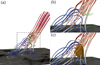 |
Fig. 2. 3D configuration of external reconnection in our simulation at t = 3t0. (a) Overview of magnetic field lines with the velocity vectors denoted by the arrows. The colors green and pink represent the positive and negative of vx, respectively. The colors of field lines have the same meaning as in Fig. 1. (b) Zoomed-in image of the reconnection region. The green arrows indicate magnetic dips. These heated curved field lines are formed through interchange reconnection between the erupting flux rope and the overlying open fields. (c) Same region as in panel b, but with the 3D curved current sheet. |
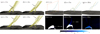 |
Fig. 3. Twist transfer and propagation after the reconnection. (a)–(d): Evolution of magnetic field lines near the outer spine. The arrows point to the curvatures of the traced field lines. The ellipses in panel g indicate the plane to calculate the averaged mass flux in Fig. C.2. (e)–(g): Evolution of the representative field line around the outer spine (blue) and the representative flux rope field line (yellow). (h)–(j): Evolution of the distribution of the twist number measured in turns in y − z plane outlined in panel a. |
Based on the SO/PHI vector magnetogram (see Appendix A for details), we performed a nonlinear force-free field (NLFFF) extrapolation to investigate the magnetic topology structure of this jet; this served as the initial magnetic field of the following MHD simulation. To account for the presence of the mini-filament indicated by observational features, we manually inserted a flux rope in the initial field that cannot be captured by the NLFFF extrapolation. The method for inserting the flux rope and the MHD model employed to simulate the jet evolution is described in Appendix B.
3. Results
Here, we show the simulation results that present similarities with observations in Figs. 1b and c. The orientation of the simulated spine (open field lines) is found to align closely with those of the observed jet outer spine. We note that the open field lines in our simulation correspond to closed field lines that connect to the distant polarities that are not included within our computational domain, thus leading to the spine appearing as open field lines and being less inclined compared to the closed structures observed. For better visualization, the magnetic field lines are colored blue to red, indicating the transition from cool to warm plasma. This allows comparison with the observed dark and bright features.
Before the eruption, the twisted flux rope resembling the mini-filament consisted of cool plasma and resided underneath the warm dome, as in the observations. As the impulsive phase begins, the flux rope expands and ascends toward the overlying dome, eventually interacting and merging with it, releasing cool material to the spine (Figs. 1b2 and c2). The propagation speed of the erupting cool material is approximately 155 km s−1, which is consistent with the speed measured in the observations (see Fig. C.1 for details). During this process, the erupting flux rope also expands and presents an untwisting motion. At the late stage of the simulation, the interaction between the flux rope and the dome persists, with cool material from the rope being continuously released and propagating along the outer spine (Figs. 1b3 and c3). The side-view snapshot also illustrates that the main body of the flux rope below the dome has been completely dissipated. The highly twisted field lines appear above the dome, and cool material is observed moving along the outer spine. The erupted cool flux shows a clear rotation motion, resembling the spiral motion of the observed dark threads accompanying the tiny jet. The strong resemblance between the simulation and observations indicates that our MHD model based on the SO/PHI high-resolution data basically reproduces the evolution of the observed tiny spiral jet.
A new result from the analysis of our MHD simulation is that an external reconnection is identified that takes place in a curved current sheet that formed at the interaction region between the erupting flux rope and the dome, as shown in Fig. 2. The velocity vectors (green and pink arrows) represent the positive and negative values of vx. One can see that these arrows point in opposite directions, indicating shear motions in the field lines, which suggests that the reconnection takes place between the twisted field and the ambient open field. Specifically, the velocities of upflows range from 60 km s−1 to 190 km s−1, consistent with the velocities of jets measured in observations (Cheng et al. 2023; Shen 2021). Moreover, the lower section of the open field presents obvious dips (pointed out by green arrows in Fig. 2b), indicating that they have just experienced a reconnection and started to be separated from the reconnection region. The increase in the temperature at magnetic dips of reconnected field lines, compared to surrounding regions, further suggests local plasma heating. Given the limitation of the energy equation we adopted, the heating is likely mainly due to the compression driven by reconnection-induced flows. We image the curved current sheet in Fig. 2c by displaying an iso-surface of J/B = 0.5 (1/Δ) that best shows the region of enhanced currents. It denotes that the reconnection region is a curved 3D current sheet formed at the interface between the rising flux rope and the dome, similar to the theoretical models of spiral jets conceived in previous ideal MHD studies (Masson et al. 2009). We emphasize that it would be impossible to determine the location and 3D geometry of the reconnection for such a tiny-scale spiral jet without the high-resolution SO/PHI-HRT data constraining the numerical model.
There is a clear transfer and propagation of magnetic twist following the external reconnection as illustrated in Fig. 3. Initially, the twist is only confined within the flux rope, with the field lines near the outer spine showing no signs of twist. Figure 3a shows the configuration when the reconnection starts. The transfer of twist from the flux rope field line to the outer spine is evident. Subsequent snapshots depict the twist carried by the curved field lines and propagating toward the higher corona (Figs. 3b–d). We also estimate the propagation speed of the twist to be about 230 km s−1. This speed is comparable to the local Alfvén speed, which is estimated to be approximately 300 km s−1 based on a magnetic field strength of B ∼ 6 G, and the plasma density of ρ ∼ 2 × 10⁻¹⁵ g cm−3 from our simulation data. This suggests that the reconnection between the twisted flux rope and the fan–spine launches a nonlinear torsional Alfvén wave that might transport energy and accelerate plasma along the outer spine (Shibata & Uchida 1986; Pariat et al. 2009; Wyper et al. 2018; Kohutova et al. 2020). We selected two representative field lines, one around the outer spine and one within the flux rope, to illustrate the evolution of twist transfer (Figs. 3e–g). Along with the evolution of the calculated twist number (Figs. 3h–j), Tw, this clearly demonstrates how the twist is carried by the open field lines, while the flux rope field lines become untwisted because of the release of twist. The effective transfer of the twist implies that such tiny spiral jets could serve as a source of, at least, some switchbacks (Bale et al. 2019; Sterling et al. 2020).
4. Summary and discussion
Thanks to the high spatial resolution magnetogram provided by PHI-HRT, we are, for the first time, able to perform a data-constrained MHD simulation to study the spiral jet’s generation mechanism from a tiny-scale fan–spine configuration. Our simulation successfully reproduces the spiral jet’s observational features, including its propagation along the outer spine and the twisting of associated dark and bright threads.
Coronal jets were proposed to be the miniature version of large-scale eruptions in previous observations (Moore et al. 2010; Sterling et al. 2015) and ideal models (Wyper et al. 2018). For large-scale eruptions, similar data-constrained and data-driven models found that the unstable flux rope is an indispensable component for a full eruption (e.g., Kliem et al. 2013). However, these results have not been justified for small-scale jets, primarily due to the limitation of the spatial resolution of the bottom boundary magnetograms they used. By utilizing higher-resolution magnetic field data (195 km per pixel), our data-constrained model effectively resolves the eruption of a very small-scale flux rope eruption spanning a scale of 10 Mm that is highly comparable with EUI observations. In particular, our MHD model confirms the external reconnection between the flux rope and the ambient field and even discloses its detailed processes, similarly to the results of Zhu et al. (2023), although they took advantage of zero-beta MHD simulations. On the other hand, the transfer of magnetic twist was previously suggested to occur in large-scale eruptions (e.g., Masson et al. 2013; Guo et al. 2024) and ideal MHD models (Pariat et al. 2009; Wyper et al. 2017). We further confirm here that the twist initially contained in the mini-flux rope can be released into the outer open fields through external reconnection. Additionally, because of the inclusion of the energy equation, even though we only consider the adiabatic process, we also reproduce the transfer of cool materials along with that of the twist, which cannot be derived in zero-beta MHD simulations.
In previous jet models, the importance of external reconnection has already been highlighted (Shibata et al. 1992; Moore et al. 2010; Sterling et al. 2015; Wyper et al. 2017). Here we further determine that the external magnetic reconnection occurs within a 3D curved current sheet, most likely collapsed from the pre-existing 3D magnetic null. We also find that such an external reconnection is the key to transferring the cool material and twist within the flux rope to the open flux close to the outer spine. A great deal of observational evidence for external reconnection, such as small-scale blobs, have been revealed by recent high-resolution imaging observations (Li et al. 2023; Cheng et al. 2023).
There is one remarkable distinction between the external reconnection we discussed here and the breakout reconnection (Wyper et al. 2017, 2018), which refers to the reconnection between the constraining field above the flux rope and the background field. In contrast, external reconnection occurs directly between the erupting flux rope and the background field, without involving a breakout process. Due to such an external reconnection, an erupting flux rope is even more easily confined due to the decrease in upward loop force, thus resulting in a failed eruption (Chen et al. 2023).
In addition, as our model represents an initial step in addressing the jet’s configuration, it does not focus too much on the thermal evolution and therefore does not contain heat conduction and radiation processes in the energy equation. Consequently, the thermal properties obtained from this numerical model are not quantitatively precise, as the heating is driven by plasma compression (−p∇⋅v), which predominantly occurs near the current-sheet regions. Since key numerical heating terms, such as Joule heating and viscous heating, are omitted in this model, the plasma cannot reach the temperature values in observations (Cheng et al. 2023). Nevertheless, the temperature changes associated with the twist transfer are evident in Fig. 2. In future work, we will focus on improving the representation of the heating process by incorporating more comprehensive source terms.
Acknowledgments
We thank the referee who helped improve the manuscript. Solar Orbiter is a space mission of international collaboration between ESA and NASA, operated by ESA. We are grateful to the ESA SOC and MOC teams for their support. The German contribution to SO/PHI is funded by the BMWi through DLR and by MPG central funds. The Spanish contribution is funded by AEI/MCIN/10.13039/501100011033/ and European Union “NextGenerationEU/PRTR” (RTI2018-096886-C5, PID2021-125325OB-C5, PCI2022-135009-2, PCI2022-135029-2) and ERDF “A way of making Europe”; “Center of Excellence Severo Ochoa” awards to IAA-CSIC (SEV-2017-0709, CEX2021-001131-S); and a Ramón y Cajal fellowship awarded to DOS. The French contribution is funded by CNES. The EUI instrument was built by CSL, IAS, MPS, MSSL/UCL, PMOD/WRC, ROB, LCF/IO with funding from the Belgian Federal Science Policy Office (BELSPO/PRODEX PEA 4000134088, 4000112292, 4000136424, and 4000134474); the Centre National d’Etudes Spatiales (CNES); the UK Space Agency (UKSA); the Bundesministerium für Wirtschaft und Energie (BMWi) through the Deutsches Zentrum für Luft- und Raumfahrt (DLR); and the Swiss Space Office (SSO). Z.F.L., X.C., and M.D.D. are funded by the Fundamental Research Funds for the Central Universities under grant 2024300348, NSFC grant 12127901, and National Key R&D Program of China under grants 2021YFA1600504 and 2022YFF0503001. The simulations in this paper were performed in the cluster system of the High Performance Computing Center (HPCC) of Nanjing University. L.P.C. gratefully acknowledges funding by the European Union (ERC, ORIGIN, 101039844). J.H.G. is supported by the China National Postdoctoral Program for Innovative Talents fellowship under Grant Number BX20240159. However, the views and opinions expressed are those of the author(s) only and do not necessarily reflect those of the European Union or the European Research Council. Neither the European Union nor the granting authority can be held responsible for them. SP acknowledges support from the projects C16/24/010 C1 project Internal Funds KU Leuven), G0B5823N and G002523N (WEAVE) (FWO-Vlaanderen), and 4000145223 (SIDC Data Exploitation (SIDEX2), ESA Prodex). We also thank Gherardo Valori for his assistance in processing the SO/PHI-HRT data.
References
- Bale, S. D., Badman, S. T., Bonnell, J. W., et al. 2019, Nature, 576, 237 [NASA ADS] [CrossRef] [Google Scholar]
- Calchetti, D., Stangalini, M., Jafarzadeh, S., et al. 2023, A&A, 674, A109 [NASA ADS] [CrossRef] [EDP Sciences] [Google Scholar]
- Chen, J., Cheng, X., Kliem, B., & Ding, M. 2023, ApJ, 951, L35 [NASA ADS] [Google Scholar]
- Cheng, X., Priest, E. R., Li, H. T., et al. 2023, Nat. Commun., 14, 2107 [Google Scholar]
- Cheung, M. C. M., De Pontieu, B., Tarbell, T. D., et al. 2015, ApJ, 801, 83 [Google Scholar]
- Chitta, L. P., Peter, H., Parenti, S., et al. 2022, A&A, 667, A166 [NASA ADS] [CrossRef] [EDP Sciences] [Google Scholar]
- Chitta, L. P., Zhukov, A. N., Berghmans, D., et al. 2023, Science, 381, 867 [NASA ADS] [CrossRef] [Google Scholar]
- Gandorfer, A., Grauf, B., Staub, J., et al. 2018, SPIE Conf. Ser., 10698, 106984N [NASA ADS] [Google Scholar]
- Guo, J. H., Ni, Y. W., Zhong, Z., et al. 2023, ApJS, 266, 3 [NASA ADS] [CrossRef] [Google Scholar]
- Guo, J. H., Linan, L., Poedts, S., et al. 2024, A&A, 683, A54 [NASA ADS] [CrossRef] [EDP Sciences] [Google Scholar]
- Hoeksema, J. T., Liu, Y., Hayashi, K., et al. 2014, Sol. Phys., 289, 3483 [Google Scholar]
- Innes, D. E., Inhester, B., Axford, W. I., & Wilhelm, K. 1997, Nature, 386, 811 [Google Scholar]
- Jiang, C., Wu, S. T., Feng, X., & Hu, Q. 2016, Nat. Commun., 7, 11522 [NASA ADS] [CrossRef] [Google Scholar]
- Joshi, R., Wang, Y., Chandra, R., et al. 2020, ApJ, 901, 94 [NASA ADS] [CrossRef] [Google Scholar]
- Kahil, F., Hirzberger, J., Solanki, S. K., et al. 2022, A&A, 660, A143 [NASA ADS] [CrossRef] [EDP Sciences] [Google Scholar]
- Keppens, R., Nool, M., Tóth, G., & Goedbloed, J. P. 2003, Comput. Phys. Commun., 153, 317 [Google Scholar]
- Keppens, R., Meliani, Z., van Marle, A. J., et al. 2012, J. Comput. Phys., 231, 718 [Google Scholar]
- Kliem, B., Su, Y. N., van Ballegooijen, A. A., & DeLuca, E. E. 2013, ApJ, 779, 129 [NASA ADS] [CrossRef] [Google Scholar]
- Kohutova, P., Verwichte, E., & Froment, C. 2020, A&A, 633, L6 [NASA ADS] [CrossRef] [EDP Sciences] [Google Scholar]
- Lemen, J. R., Title, A. M., Akin, D. J., et al. 2012, Sol. Phys., 275, 17 [Google Scholar]
- Li, Z. F., Cheng, X., Ding, M. D., et al. 2023, A&A, 673, A83 [NASA ADS] [CrossRef] [EDP Sciences] [Google Scholar]
- Liu, J., Wang, Y., Shen, C., et al. 2015, ApJ, 813, 115 [NASA ADS] [CrossRef] [Google Scholar]
- Masson, S., Pariat, E., Aulanier, G., & Schrijver, C. J. 2009, ApJ, 700, 559 [Google Scholar]
- Masson, S., Antiochos, S. K., & DeVore, C. R. 2013, ApJ, 771, 82 [NASA ADS] [CrossRef] [Google Scholar]
- Metcalf, T. R. 1994, Sol. Phys., 155, 235 [Google Scholar]
- Metcalf, T. R., Leka, K. D., Barnes, G., et al. 2006, Sol. Phys., 237, 267 [Google Scholar]
- Moore, R. L., Cirtain, J. W., Sterling, A. C., & Falconer, D. A. 2010, ApJ, 720, 757 [Google Scholar]
- Moore, R. L., Sterling, A. C., Cirtain, J. W., & Falconer, D. A. 2011, ApJ, 731, L18 [NASA ADS] [CrossRef] [Google Scholar]
- Müller, D., St. Cyr, O. C., Zouganelis, I., et al. 2020, A&A, 642, A1 [Google Scholar]
- Nayak, S. S., Bhattacharyya, R., Prasad, A., et al. 2019, ApJ, 875, 10 [Google Scholar]
- Pariat, E., Antiochos, S. K., & DeVore, C. R. 2009, ApJ, 691, 61 [Google Scholar]
- Pariat, E., Antiochos, S. K., & DeVore, C. R. 2010, ApJ, 714, 1762 [NASA ADS] [CrossRef] [Google Scholar]
- Pesnell, W. D., Thompson, B. J., & Chamberlin, P. C. 2012, Sol. Phys., 275, 3 [Google Scholar]
- Priest, E. R., & Syntelis, P. 2021, A&A, 647, A31 [EDP Sciences] [Google Scholar]
- Raouafi, N. E., Patsourakos, S., Pariat, E., et al. 2016, Space Sci. Rev., 201, 1 [Google Scholar]
- Rochus, P., Auchère, F., Berghmans, D., et al. 2020, A&A, 642, A8 [NASA ADS] [CrossRef] [EDP Sciences] [Google Scholar]
- Scherrer, P. H., Schou, J., Bush, R. I., et al. 2012, Sol. Phys., 275, 207 [Google Scholar]
- Schmieder, B., Archontis, V., & Pariat, E. 2014, Space Sci. Rev., 186, 227 [NASA ADS] [CrossRef] [Google Scholar]
- Shen, Y. 2021, Proc. R. Soc. London Ser. A, 477, 217 [NASA ADS] [Google Scholar]
- Shibata, K., & Uchida, Y. 1986, Sol. Phys., 103, 299 [NASA ADS] [CrossRef] [Google Scholar]
- Shibata, K., Ishido, Y., Acton, L. W., et al. 1992, PASJ, 44, L173 [Google Scholar]
- Shibata, K., Nakamura, T., Matsumoto, T., et al. 2007, Science, 318, 1591 [Google Scholar]
- Shimojo, M., & Shibata, K. 2000, Adv. Space Res., 26, 449 [NASA ADS] [Google Scholar]
- Sinjan, J., Calchetti, D., Hirzberger, J., et al. 2022, SPIE Conf. Ser., 12189, 121891J [NASA ADS] [Google Scholar]
- Solanki, S. K., del Toro Iniesta, J. C., Woch, J., et al. 2020, A&A, 642, A11 [NASA ADS] [CrossRef] [EDP Sciences] [Google Scholar]
- Sterling, A. C., Moore, R. L., Falconer, D. A., & Adams, M. 2015, Nature, 523, 437 [NASA ADS] [CrossRef] [Google Scholar]
- Sterling, A. C., Moore, R. L., Panesar, N. K., & Samanta, T. 2020, J. Phys. Conf. Ser., 1620, 012020 [Google Scholar]
- Tian, H., Zhu, X., Peter, H., et al. 2018, ApJ, 854, 174 [NASA ADS] [CrossRef] [Google Scholar]
- Titov, V. S., Török, T., Mikic, Z., & Linker, J. A. 2014, ApJ, 790, 163 [NASA ADS] [CrossRef] [Google Scholar]
- Titov, V. S., Downs, C., Mikić, Z., et al. 2018, ApJ, 852, L21 [NASA ADS] [CrossRef] [Google Scholar]
- Wang, Y. M., Sheeley, N. R., Socker, D. G., et al. 1998, ApJ, 508, 899 [NASA ADS] [CrossRef] [Google Scholar]
- Wyper, P. F., & DeVore, C. R. 2016, ApJ, 820, 77 [Google Scholar]
- Wyper, P. F., Antiochos, S. K., & DeVore, C. R. 2017, Nature, 544, 452 [Google Scholar]
- Wyper, P. F., DeVore, C. R., & Antiochos, S. K. 2018, ApJ, 852, 98 [Google Scholar]
- Wyper, P. F., DeVore, C. R., & Antiochos, S. K. 2019, MNRAS, 490, 3679 [NASA ADS] [CrossRef] [Google Scholar]
- Xia, C., Teunissen, J., El Mellah, I., Chané, E., & Keppens, R. 2018, ApJS, 234, 30 [Google Scholar]
- Yokoyama, T., & Shibata, K. 1996, PASJ, 48, 353 [Google Scholar]
- Zhu, J., Guo, Y., Ding, M., & Schmieder, B. 2023, ApJ, 949, 2 [NASA ADS] [CrossRef] [Google Scholar]
Appendix A: Instruments
We used the calibrated L2 174 Å images on March 3, 2022, obtained from HRIEUV on board Solar Orbiter. At that time, Solar Orbiter was located at a distance of 0.50 AU from the Sun and almost aligned with the Sun-Earth line, with an angular separation of approximately 7 degrees. The dataset1 was taken between 09:40 UT and 10:40 UT with a cadence of 5 s. The pixel size is 0.492″, corresponding to a spatial scale of about 195 km. The vector magnetogram used in the magnetic field extrapolation and numerical simulation was acquired by the High-Resolution Telescope (SO/PHI-HRT; Gandorfer et al. 2018; Solanki et al. 2020) of PHI on board Solar Orbiter. The dataset spans the same observational period as EUI, with a temporal cadence of 300 s. The images have a spatial resolution of 0.5″ per pixel, corresponding to ≃200 km on the Sun. They are calibrated using the SO/PHI-HRT on-ground pipeline (Sinjan et al. 2022; Calchetti et al. 2023). The ambiguity in the transverse component of the magnetic field was removed using an adapted version of the ME0 method (Metcalf 1994), as implemented in the pipeline of the Helioseismic and Magnetic Imager (HMI; Scherrer et al. 2012) on board SDO (Metcalf et al. 2006; Hoeksema et al. 2014).
We removed the jitter in both datasets using a cross-correlation method (see Appendix A.1 in Chitta et al. 2022 for details). We note that the fields of view (FOVs) these two datasets are not identical. We adopted a cross-correlation approach to coregister the images of the HRIEUV and HRT. Following the methodology outlined by Kahil et al. (2022), we initially aligned the HRILya image with the HRIEUV image and then aligned the HRT image with the HRILya image. HRILya images the Sun in Ly-a at 1215 Å and shows the chromosphere. This procedure ensures that the datasets of the HRT and HRIEUV are accurately co-aligned. Upon examining the coaligned images, we find a good match in position between the brightenings and regions with strong magnetic fields, as evident from the comparison between Fig. 1 in Cheng et al. (2023) and Fig. B.1(a).
Appendix B: Adiabatic MHD model
The twisted flux rope was reconstructed by the regularized Biot–Savart laws (RBSL) method (Titov et al. 2018). Four key parameters govern this method: the flux rope path; flux rope radius, a; electric current, I; and toroidal magnetic flux, F. We outlined the projected flux rope path by following the mini-filament spine as indicated by the blue dashed curve in Fig. 1(a1). This path was selected based on observations of the dark lane in this region, and the resulting extrapolations yield a dome structure that is consistent with the observation. The radius was set as 0.7 Mm according to the apparent width of the mini-filament. We first derived the reference equilibrium current-field intensity (I0) according to Eq. (7) in Titov et al. (2014), denoted as I0 = 8.5 × 10⁹ A. After some tests and experiments, we selected I = 1.6I0. As a result, the residual Lorentz force was able to directly trigger the eruption of the inserted flux rope. Then, the toroidal flux F was computed by Eq. (12) in Titov et al. (2018). The height of the null point, as measured by Cheng et al. (2023), is remarkably low, consistent with our NLFFF extrapolation results, being only about 1-2 Mm above the photosphere. This suggests that the flux rope resides in the chromosphere, which does not conform to a force-free condition. As a result, we adopted an unstable flux rope resembling the eruptive mini-filament to initiate the spiral jet.
The initial 3D magnetic field in our MHD simulations is presented in Fig. B.1. Specifically, this structure reveals a dome containing a 3D null, representing the fan separatrix surface of magnetic field lines enclosing the inserted flux rope and connecting toward the polarity outside the simulation box. This topology is consistent with the suggestion in Cheng et al. (2023). Then, we ran the numerical simulation to derive the magnetic field evolution. The governing equations are as follows:
 (B.1)
(B.1)
 (B.2)
(B.2)
 (B.3)
(B.3)
 (B.4)
(B.4)
Here ρ is density, v is the velocity, B is the magnetic field, eint = p/(γ − 1) is the internal energy, and g = −gez is the gravity acceleration. The 3D MHD equations are numerically solved with MPI-AMRVAC. The computational domain is 58.4 × 58.4 × 30 Mm3, resolved by a uniform grid with 300 × 300 × 600 cells. This setup yields a horizontal resolution of 195 km, maintaining the high resolution of the magnetogram, and a vertical resolution of 50 km, sufficient to accurately resolve the flux rope structure of the mini-filament in observations. The cadence of saved data in our simulation is t0 = 0.3τ, where τ ≈ 86s is the Alfvén time.
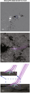 |
Fig. B.1. Overview of the surface magnetic field. (a) PHI line-of-sight (LOS) magnetogram showing the magnetic field distribution of the associated main active region before the eruption. (b) 3D magnetic field configuration, traced by the magnetic field lines, showing the initial condition of data-constrained 3D MHD simulation. The background image is the zoom-in of the PHI LOS magnetogram, as marked by a blue square in panel (a). (c) Same as panel (b), but for the side view and with a small panel more clearly showing the flux rope. |
Appendix C: Propagation of cool material
Figure C.1 clearly illustrates the propagation of an erupting blob with dense plasma along the outer spine. Initially, the flux rope contains cool, dense plasma. After the reconnection, the dense plasma is released to the outer spine and subsequently propagates toward the upper corona.
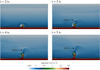 |
Fig. C.1. Distribution of density during the tiny jet showing the propagation of an erupting blob in the plane vertical to the spine. |
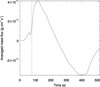 |
Fig. C.2. Averaged mass flux through the plane indicated in Fig. 3 during the whole process. The red dashed line indicates the moment reconnection occurs. |
Furthermore, we find that the reconnection facilitates the transfer of cool material originally included within the flux rope to the upper corona. Figure C.2 illustrates the averaged mass flux through a plane just above the reconnection region (z ∼ 10 Mm), with the dashed line indicating the onset time of reconnection. The mass flux is calculated by F = ρv. A significant increase in mass flux is observed after the external reconnection, and a peak is reached quickly in 40 seconds. This indicates that the effective mass transfer toward the upper corona is driven by reconnection. The effective mass transfer occurs on a timescale of approximately 5 minutes, aligning with the timescale of fan reconnection (Cheng et al. 2023). We note that our computational domain is significantly smaller in the vertical extent than the coronal pressure scale height. Hence, within the framework of our model, the ejected material does not form the solar wind, but falls back to the surface (at ∼250 s in Fig. C.2).
All Figures
|
Fig. 1. Comparison between observations and simulations at three instances. (a) EUI 174 Å images displaying the temporal evolution of the spiral jet eruption with arrows indicating dark threads. The blue dashed curve in panel a1 indicates the path of the inserted flux rope. (b) Temporal evolution of 3D magnetic field lines as viewed from the top. (c) Same as panel b, but as viewed from the side. The lines in blue and red correspond to cold and warm plasma, respectively. The red dashed lines indicate the plane in Fig. C.1. |
| In the text | |
|
Fig. 2. 3D configuration of external reconnection in our simulation at t = 3t0. (a) Overview of magnetic field lines with the velocity vectors denoted by the arrows. The colors green and pink represent the positive and negative of vx, respectively. The colors of field lines have the same meaning as in Fig. 1. (b) Zoomed-in image of the reconnection region. The green arrows indicate magnetic dips. These heated curved field lines are formed through interchange reconnection between the erupting flux rope and the overlying open fields. (c) Same region as in panel b, but with the 3D curved current sheet. |
| In the text | |
|
Fig. 3. Twist transfer and propagation after the reconnection. (a)–(d): Evolution of magnetic field lines near the outer spine. The arrows point to the curvatures of the traced field lines. The ellipses in panel g indicate the plane to calculate the averaged mass flux in Fig. C.2. (e)–(g): Evolution of the representative field line around the outer spine (blue) and the representative flux rope field line (yellow). (h)–(j): Evolution of the distribution of the twist number measured in turns in y − z plane outlined in panel a. |
| In the text | |
|
Fig. B.1. Overview of the surface magnetic field. (a) PHI line-of-sight (LOS) magnetogram showing the magnetic field distribution of the associated main active region before the eruption. (b) 3D magnetic field configuration, traced by the magnetic field lines, showing the initial condition of data-constrained 3D MHD simulation. The background image is the zoom-in of the PHI LOS magnetogram, as marked by a blue square in panel (a). (c) Same as panel (b), but for the side view and with a small panel more clearly showing the flux rope. |
| In the text | |
|
Fig. C.1. Distribution of density during the tiny jet showing the propagation of an erupting blob in the plane vertical to the spine. |
| In the text | |
|
Fig. C.2. Averaged mass flux through the plane indicated in Fig. 3 during the whole process. The red dashed line indicates the moment reconnection occurs. |
| In the text | |
Current usage metrics show cumulative count of Article Views (full-text article views including HTML views, PDF and ePub downloads, according to the available data) and Abstracts Views on Vision4Press platform.
Data correspond to usage on the plateform after 2015. The current usage metrics is available 48-96 hours after online publication and is updated daily on week days.
Initial download of the metrics may take a while.