| Issue |
A&A
Volume 693, January 2025
|
|
|---|---|---|
| Article Number | A152 | |
| Number of page(s) | 11 | |
| Section | Astrophysical processes | |
| DOI | https://doi.org/10.1051/0004-6361/202451815 | |
| Published online | 14 January 2025 | |
Crab pulsar: IXPE observations reveal unified polarization properties in the optical and soft X-ray bands
1
Institut de Recherche en Astrophysique et Planétologie, UPS-OMP, CNRS, CNES, 9 Avenue du Colonel Roche, BP 44346 31028 Toulouse Cedex 4, France
2
University of British Columbia, Vancouver, BC, Canada
3
INAF Istituto di Astrofisica e Planetologia Spaziali, Via del Fosso del Cavaliere 100, 00133 Roma, Italy
4
INAF Osservatorio Astrofisico di Arcetri, Largo Enrico Fermi 5, 50125 Firenze, Italy
5
Dipartimento di Fisica e Astronomia, Università degli Studi di Firenze, Via Sansone 1, 50019 Sesto, Fiorentino (FI), Italy
6
Istituto Nazionale di Fisica Nucleare, Sezione di Firenze, Via Sansone 1, 50019 Sesto, Fiorentino (FI), Italy
7
Guangxi Key Laboratory for Relativistic Astrophysics, School of Physical Science and Technology, Guangxi University, Nanning 530004, China
⋆ Corresponding author; This email address is being protected from spambots. You need JavaScript enabled to view it.
Received:
6
August
2024
Accepted:
4
December
2024
Abstract
We present a phase-dependent analysis of the polarized emission from the Crab pulsar based on three sets of observations by the Imaging X-ray Polarimetry Explorer (IXPE). We found that a phenomenological model involving a simple linear transformation of the Stokes parameters adequately describes the IXPE data. This model enabled us to establish a connection between the polarization properties of the Crab pulsar in the optical and soft X-ray bands for the first time, which suggests a common underlying emission mechanism in these bands that likely is synchrotron radiation. In particular, the phase-dependent polarization degree in X-rays for the pure pulsar emission shows similar features, but is reduced by a factor ≈(0.46 − 0.56) compared to the optical band (when we accounted for the contribution of the knot in the optical), which implies an energy-dependent polarized emission. Using this model, we also studied the polarization angle swing in the X-rays and identified a potentially variable phase shift at the interpulse relative to the optical band, alongside a phase shift that is marginally consistent with zero and persists at the main pulse. While the origin of this variability is unknown and presents a new challenge for the theoretical interpretation, our findings suggest that the emission mechanism for the main pulse is likely located far from the neutron star surface, perhaps near to or beyond the light cylinder, and that it does not operate in the inner magnetosphere, where vacuum birefringence is expected to be at work. Ignoring the phase shifts would result in identical phase-dependent polarization angles between the optical and X-ray bands for the pure pulsar emission.
Key words: polarization / pulsars: individual: Crab Pulsar
© The Authors 2025
 Open Access article, published by EDP Sciences, under the terms of the Creative Commons Attribution License (https://creativecommons.org/licenses/by/4.0), which permits unrestricted use, distribution, and reproduction in any medium, provided the original work is properly cited.
This article is published in open access under the Subscribe to Open model. This email address is being protected from spambots. You need JavaScript enabled to view it. to support open access publication.
1. Introduction
The recently launched (December 2021) Imaging X-ray Polarimetry Explorer mission (IXPE) opened a new window for studying polarized soft X-ray sources (2−8 keV) in extreme astrophysical environments (Weisskopf et al. 2022). One of the main targets of the IXPE Long-term plan (LTP) is the Crab pulsar wind nebula (PWN). This is one of the most frequently studied X-ray sources that has also been subject to a polarimetric analysis with various instruments (e.g., Weisskopf et al. 1978; Forot et al. 2008; Chauvin et al. 2013, 2017; Vadawale et al. 2018; Feng et al. 2020; Long et al. 2021; Li et al. 2022). It consists of a fast spinning (P = 33.7 ms) and highly magnetized (B = 3.8 × 10¹² G) neutron star (Crab pulsar, PSR B0531+21, PSR J0534+2200) that accelerates particles that power a PWN (G184.6−5.8). Although they are considered sources of nonthermal radiation (synchrotron, curvature radiation, and inverse-Compton processes), the mechanism of pulsar emission and its location remain subject of debate (for reviews see e.g., Bühler & Blandford 2014; Harding 2019; Philippov & Kramer 2022). As part of the LTP, three sets of observations were performed for the Crab PWN. The first observation, made during cycle 1, had an exposure time of ∼90 ks, while the second and third observations, requested as follow-up during cycle 2, had exposure times of ∼150 ks and ∼60 ks, respectively. These observations were made on 21 March 2022, 1 April 2023, and 9 October 2023.
Based on the first observation, the IXPE team reported a polarimetric analysis of Crab PWN focusing on the nebula emission, which yielded an integrated polarization degree PD ∼ 20%. In addition, preliminary analyses found a low polarized emission from the Crab pulsar with a maximum PD ∼ 15% at the core of the main peak (Bucciantini et al. 2023), as well as indications of a fast polarization angle swing ∼100° −150° (Wong et al. 2023). Later, an analysis that included all three IXPE observations of the Crab PWN was performed by Wong et al. (2024), who reported results that were consistent with those reported by Bucciantini et al. (2023). Additionally, Wong et al. (2024) identified (i) a well-defined S-shaped polarization angle swing at the main peak, (ii) polarization in six bins in the main pulse and 2 phase bins in the interpulse (out of a total of 20 phase bins), and (iii) substantial differences in the phase-dependent polarization properties for the main peak and the interpulse compared to those observed in the optical band (Słowikowska et al. 2009). In particular, they concluded that different emission mechanisms or locations might explain the optical and X-ray polarized emission. In contrast, as discussed below, our analysis suggests a common emission mechanism in the two bands. This differs from the conclusions of Wong et al. (2024) and offers new insights into the magnetospheric emission of the Crab pulsar.
Our main goal is to examine the pulsed emission from the Crab pulsar, with a particular focus on studying the polarization angle swing observed by IXPE. The high magnetic field of the Crab pulsar, its short rotational period, the relatively close distance of ∼2 kpc (Trimble 1973), and the bright pulsed X-ray flux F(2 − 10 keV) ∼ 2.7 × 10⁻⁹ erg cm−2 s−1 make it an ideal X-ray source for studying quantum electrodynamics (QED) effects. A strong magnetic field is expected to modify the properties of the vacuum by inducing the temporary formation of virtual electron-positron pairs, which can lead to the appearance of vacuum birefringence (Heisenberg & Euler 1936; Weisskopf 1936; Schwinger 1951), a phenomenon that remains unobserved experimentally. (An astrophysical signature of this phenomenon was potentially obtained in the optical band for RX J1856.5−3754 by Mignani et al. 2017, however). Under vacuum birefringence, electromagnetic waves with different energies and polarization modes propagate at different speeds and decouple at different locations within the pulsar magnetosphere. Consequently, if the emission mechanism takes place well inside the light cylinder, it is expected that the rapid rotation of the magnetosphere (P ≲ 0.1 s) will induce a phase shift in the polarization angle between observations at different energy bands (Heyl & Shaviv 2000).
In a fast-rotating pulsar, the effects of vacuum birefringence compete with the magnetospheric plasma. For a pulsar with a Goldreich-Julian charge density nGJ (Goldreich & Julian 1969), the birefringence effects arising from the vacuum dominate those resulting from the plasma density for photon energies that are sufficiently high (Heyl & Shaviv 2000),
 (1)
(1)
Therefore, observations in optical and higher-energy ranges can enable us to investigate the vacuum birefringence in magnetized neutron stars, such as the Crab pulsar, and to probe the magnetosphere of these sources.
Extensive studies of the polarization properties of the Crab pulsar were conducted over the past decades in the optical band (see e.g. Cocke et al. 1969; Kristian et al. 1970; Smith et al. 1988; Słowikowska et al. 2009; Moran et al. 2013) (for general reviews of multiwavelength polarimetry of pulsars, see also Mignani 2018; Harding 2019; Bucciantini et al. 2024). The most precise phase-dependent measurements were carried out by Słowikowska et al. (2009) using the high-speed photopolarimeter Optical Pulsar TIMing Analyser (OPTIMA) at approximately 2 eV. On the other hand, the IXPE mission operates at sufficiently high energies, in the range of 2 − 8 keV, and its sensitivity is high enough to carry out phase-dependent polarimetric observations. It is therefore now possible to search for phase shifts in the polarization angle of the Crab pulsar between the optical and X-ray bands.
We develop a phenomenological model based on the phase-dependent polarimetric observations of the Crab pulsar in the optical band. This energy range is closest to the soft X-rays, where high-quality polarization measurements were obtained. By applying a linear transformation of the Stokes parameters in the optical band, we can provide a fairly good description of the IXPE phase-dependent observations of the Crab pulsar in the X-ray band. This suggests that the underlying emission mechanisms that operate in these bands are likely the same. Furthermore, motivated by the search for a signal of vacuum birefringence (Heyl & Shaviv 2000), we include two additional free parameters in the model: A phase shift in the polarization angle swing at the main pulse, and one at the interpulse, and we fit them to IXPE observations1. While the phase shift at the main pulse is marginally consistent with zero for the three IXPE observations of the Crab pulsar, the phase shift at the interpulse varies between different observations. While this variability is likely a new feature in the polarization properties of the Crab pulsar in the X-rays, the polarization angle swing in the main peak suggests that the emission mechanism that produces the main peak is not affected by vacuum birefringence (within the polarization limiting radius2), and therefore, its location is well outside the magnetosphere, perhaps close to or beyond the light cylinder.
The paper is organized as follows. In Sect. 2 we present our model for the Stokes parameters, the implementation of the phase shift in the polarization angle, and the fit to the IXPE data. The discussion and conclusions are presented in Sect. 3.
2. Method
The Crab pulsar is characterized by a double-pulsed emission per cycle that is observable almost across the whole electromagnetic spectrum, from radio waves to high-energy gamma rays (for a review see e.g. Bühler & Blandford 2014). The locations of the peak for the main pulse and interpulse3 show relatively small variations in phase between the optical (Słowikowska et al. 2009) and the X-ray band (Weisskopf et al. 2011), with a peak-to-peak separation of ∼0.4 cycles. In the optical band and higher energies, a bridge emission is observed between the peaks. Furthermore, the off-pulse emission (or DC region) is also typically characterized as that of the pulse profile minimum, where the emission from the knot (in the optical) or the PWN (in X-rays) becomes prominent. In order to perform a polarimetric analysis, previous studies of the Crab pulsar involved subtracting the Stokes parameters associated with the off-pulsed emission from those of the pulsar (e.g., Słowikowska et al. 2009; Bucciantini et al. 2023). However, we take the opposite approach. We directly extract the pulsed Stokes parameters from the IXPE data and then compare them with a pulsar model that accounts for the contribution from the PWN (or for any form of constant polarization) as described below.
2.1. Linear transformation
In order to perform an in-depth study of the phase-dependent polarization properties of the Crab pulsar, we built a phenomenological model assuming that the main features of the Stokes parameters for the pulsar emission in the optical band (Słowikowska et al. 2009) are preserved in the X-ray band. We also allowed the IXPE polarimetric features to stretch or contract when compared to optical observations, which can be expressed as a linear transformation of the Stokes parameters, given by
 (2)
(2)
with
 (3)
(3)
where the diagonal matrix A quantifies a deviation from the pulsar Stokes parameters between the optical and X-rays, while the vector B quantifies the contribution from the nebula emission or any additional form of constant polarization, such as spurious polarization (although this should already be removed), and background, both celestial and instrumental. For the A matrix, we repeated the β coefficient in the diagonal and did not consider off-diagonal terms in order to avoid introducing a rotation or mixing of the Stokes parameters of the pulsar between the optical and X-rays, which not justified a priori. Here, (IV, QV, UV) is the set of Stokes parameters in the optical band (see Appendix A), which are likely dominated by pulsar emission at almost all phases (with the exception of the DC component, as discussed below), and (IX, QX, UX) correspond to the Stokes parameters in the IXPE X-ray band, which have a relatively large nebula component due to the broad instrumental PSF.
Nevertheless, the I Stokes parameter for the pulsar itself in the X-ray range was determined previously, with minimum contamination from the nebula, based on observations conducted by the Chandra X-ray observatory (Weisskopf et al. 2011). Therefore, because we aimed to perform our analysis in the X-rays, we used Crab pulsar intensity Stokes from the Chandra observations (which is different from the intensity Stokes from IXPE observations), but preserved the polarimetric characteristics observed in the optical band, that is, the phase-dependent polarization degree and the polarization angle. In the linear transformation above, we accomplished this by substituting SV by
 (4)
(4)
where ICX corresponds to the Chandra X-ray intensity of the pulsar (see Appendix B), and  and ψV = (1/2)arctan(UV/QV) are the polarization fraction and polarization angle in the optical band, respectively. As discussed in Słowikowska et al. (2009), the optical Stokes parameters include a DC component, which is probably due to the PWN knot. However, the magnitude of this contribution is unclear. Therefore, we also tested a scenario in which we removed 90% of the DC component from the optical Stokes as follows:
 (5)
(5)
 (6)
(6)
 (7)
(7)
where IV, dc, QV, dc, and UV, dc are the optical Stokes parameters at phase ≈0.8.
2.2. Polarization angle including phase shifts
If the emission mechanism takes place well inside the light cylinder (or near the NS surface), vacuum birefringence is expected to induce a phase shift in the polarization angle that depends on the energy and rotational phase of the pulsar (e.g., the polarization angle swing for low-frequency emission lags that for higher-frequency radiation). Phase shifts were computed, for example, for a corotating dipole model and a Deutsch model by Heyl & Shaviv (2000). The two models showed that the phase variation for the polarization angle within the energy range of IXPE is very small compared to the variation between the optical V-band and soft X-rays. Therefore, we investigated potential phase shifts for the polarization angle as the difference in phase associated with two representative energies:
-
(i)
E = 2 eV, which corresponds to the optical V-band of the polarimetric observations of the Crab pulsar (Słowikowska et al. 2009), and
-
(ii)
E = 3 keV, which corresponds to the energy for the maximum sensitivity of IXPE.
As mentioned above, the phase shift also depends on the rotational phase of the pulsar. In principle, the signal of the phase shift is stronger at the peak of the pulse and interpulse, where the polarization angle also exhibits its maximum swing. In the following, we define these two peaks as located within two broad rotational phase intervals:
-
(i)
for phases inside the interval [ϕ1min, ϕ2min] or interpulse, and
-
(ii)
for phases outside [ϕ1min, ϕ2min] or main pulse,
where ϕ1min = 0.138 and ϕ2min = 0.683 correspond to the two local minima in the intensity Stokes parameter ICX as observed by Chandra. In the case of IXPE observations, the X-ray emission is substantially affected by the nebula emission around ϕ1min and ϕ2min. Therefore, and for simplicity, we ignored potential continuous phase-dependent phase shifts. For the pulsar in the X-rays, we then implemented the phase-dependent polarization angle model including two independent phase shifts with respect to the optical band as follows:
 (8)
(8)
where ψV corresponds to the phase-dependent polarization angle model from optical observations (V band), ϕ is the rotational phase of the pulsar, and δI and δP correspond to the phase shifts at the interpulse and main pulse, respectively. (In the following, positive phase shifts mean that the polarization angle swing for the optical band lags the X-ray band). From Heyl & Shaviv (2000), the theoretical expectations for the phase shift due to vacuum birefringence are typically δP = 0.91% and δI = 1.74% at the pulse and interpulse peaks, respectively. Figure 1 shows the model for the polarization angle including negative and positive phase shifts in the range [ − 5, 5]%.
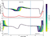 |
Fig. 1. Phenomenological polarization angle model, φX, for the pulsar in the X-rays considering positive and negative phase shifts from −5% to 5% at the interpulse (upper panel) and main pulse (lower panel). For reference, the dotted black line shows the optical (V-band) polarization angle, and the solid red curve shows the I Stokes (V-band, with arbitrary normalization) from Słowikowska et al. (2009). The phase shifts are applied within the boundaries indicated by the vertical dashed blue lines. |
By including the phase shifts in the polarization angle, the full optical-to-X-ray linear transformation of the Stokes parameters can be expanded as
 (9)
(9)
 (10)
(10)
 (11)
(11)
We derived the whole set of parameters {α,β,bI,bQ,bU,δI,δP}4 after fitting the model to IXPE polarimetry data. Consequently, the full polarization angle model for the pulsar including nebula emission is ψ = (1/2)arctan(UX/QX), and the polarization degree model is  .
.
2.3. Data reduction, fitting procedure, and MCMC
The data reduction for the first set of observations was summarized in the method section of Bucciantini et al. (2023). The second and third sets of IXPE observations were reduced in a similar manner, that is, we used the IXPEOBSSIM package (Baldini et al. 2022) to perform the energy calibration, correct for the detector WCS, for the aspect solution, and for the unweighted analysis. We used a circular subtraction region with a radius of 20″ and selected photons in the 2 − 4 keV range (corresponding to the maximum IXPE sensitivity and to avoid nebula contamination that becomes dominant at higher energies). We corrected for the barycenter with BARYCORR FTOOL, and the photons were phase-folded using a Lomb-Scargle periodogram. It is well known that the locations of the main peak at different energy bands in the Crab pulsar are slightly misaligned (by about 1% in phase), and the optical, X-ray, and gamma ray peaks lead the radio peak. In the following, we set phase zero at 0.99 relative to the radio peak for the main peak5 (see also, Bucciantini et al. 2023).
Differently from Bucciantini et al. (2023), the binned data were analysed using an equipopulated binning to produce a constant MDP99 throughout all rotational phases of the pulsar6. This approach was employed to prevent any modulation of the MDP99 that occurs, for example, for a equi-spaced binning in phase (because the Crab pulsar is strongly double-peaked in counts over a rotational cycle). We used the PCUBE algorithm to produce 40 phase bins for the I, Q, U Stokes parameters and for the polarization degree and angle. As shown in the second panel of Figure 2, all polarization degree data points are above the MDP99.
We fit the model presented in the previous section to the IXPE data. We are interested in the polarization properties of the Crab pulsar, and we therefore minimized the effects of the modulation contained in the intensity Stokes and computed the χ2 statistic as
 (12)
(12)
where
 (13)
(13)
correspond to the normalized Stokes model (binned according to the data), and q and u correspond to the normalized IXPE Stokes data. σq and σu are the associated data errors. Equation (13) depends on Equations (9), (10) and (11), for which the pulsar model ICX is folded according to the IXPE response functions (RMF and ARF), including approximately the effects of the ISM absorption (Wilms et al. 2000) with a fixed value NH = 3.27 × 1021 cm−2 (Weisskopf et al. 2011). The IX Stokes was fit separately, and the results for the coefficients α and bI are summarized in Table 1.
Summary of the model parameters we fit to three separate observations of the Crab pulsar by IXPE.
In order to build posterior distributions of the best-fit parameters, we used an MCMC analysis (Foreman-Mackey et al. 2013), which also helped us to verify potential multiple local minima and choose the best space of parameter solutions. By visual inspection of the data, it is already clear that no large phase shift is present in the polarization angle at the main pulse. Therefore, we set hard boundaries to search for a phase shift δP in the range [ − 5, 5%]. For the interpulse, visual inspection does not provide clear evidence for or against a phase shift. This prompted us to allow broader boundaries for δI in the range [ − 30, 30]%. In the following, we built posterior distributions using 100 walkers and 10 000 steps for all MCMC analyses. We discarded the initial 20% of the iterative steps.
3. Discussion and conclusions
Figure 2 shows the best-fit model to the data for the first IXPE observation and Figure 3 shows the associated posterior distribution. Similarly, Figures 4 and 5 show the results for the second IXPE observation, and Figures 6 and 7 show the results for the third IXPE observation. In all cases, the model describes the data satisfactorily for almost all the rotational phases of the pulsar, except for the phases around the main pulse ≈0.95 − 1.00. In this specific phase range, the model and the data differ, which is particularly evident in the normalized Stokes Q/I for the third observations. This deviation propagates to the polarization angle, which shows a relatively large swing that our model is unable to reproduce accurately. Nevertheless, it is important to note that this minor discrepancy does not impact the overall results and demonstrates for the first time that a simple linear transformation of the Stokes parameters from the optical to the X-ray band is sufficient to explain the IXPE observations of the Crab pulsar. This therefore suggests that a common mechanism likely causes the emission in the optical and X-ray bands. This result provides further observational confirmation for previous theoretical studies based on synchrotron radiation, which provided a fairly good description of the optical pulsed emission and polarization (see e.g., Pétri & Kirk 2005) and of the SED between the optical and X-ray of Crab pulsar (see e.g., Harding et al. 2021).
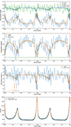 |
Fig. 2. Best-fit model to the first observation of the Crab pulsar by IXPE in the 2 − 4 keV range. The data reduction was performed with the IXPEOBSSIM package considering equipopulated binning for the Stokes parameters (first panel), and for the polarization degree (second panel) and polarization angle (third panel). The green line in the second panel corresponds to MDP99. The solid gray lines in the first three panels correspond to the best-fit model without a phase shift. The orange and gray arrows highlight the polarization angle swing at the interpulse with and without a phase shift, respectively. For completeness, we include the pulse profile with 400 equispaced bins (fourth panel). |
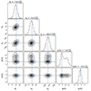 |
Fig. 3. Posterior distributions for the first observation of the Crab pulsar by IXPE. The model parameters include the phase shifts at the main pulse (δP) and interpulse (δI). The MCMC analysis was performed using 100 walkers and 10 000 steps. The blue lines show the solution obtained with a minimization routine. |
Our results represent a step forward compared to the recent analysis of the Crab by Wong et al. (2024). They applied a simultaneous fitting technique (Wong et al. 2023) to the IXPE data, a sensitive method based on Chandra X-ray observations to model the pulsar (and nebula). This enabled them to characterize the phase-dependent polarization properties in the X-rays. They then compared the phase-dependent polarization properties in the optical (Słowikowska et al. 2009) with those found in the X-rays and reported a substantial difference between the two. This led them to conclude, in contrast to our results, that different emission mechanisms (or sites) cause the optical and X-ray emissions of the Crab pulsar. However, unlike our work, they did not report further attempts to establish a relation between the optical and X-ray phase-dependent polarization properties.
Our phenomenological model (Equations 9, 10, and 11) and the results presented in Table 1 show that when the nebula contribution is neglected, that is, when we set bI = bQ = bU = 0, then the (phase-dependent) polarization degree for the pulsar alone can be simply written as p = pV β/α ≈ 0.46 pV. This implies that in the IXPE band, the Crab pulsar is about 54% less polarized than in the optical band, suggesting an underlying energy-dependent polarized emission. Similarly, without the nebula contribution, the polarization angle for the pulsar in the IXPE band is found to be similar to that in the optical band, but with a phase shift at the interpulse that is discussed below. On the other hand, we also obtained that the polarization degree for the nebula component without the pulsar contribution is  , while the polarization angle is (1/2)arctan(bU/bQ)≈135°, as is also clearly evident in Figure 2, 4, and 6.
Notably, by applying the model mentioned above, we also found a variable phase shift at the interpulse  ,
,  , and
, and  (≈2σ, 8σ, and within 1σ away from zero, respectively) when we separately performed7 the MCMC analysis for the three sets of IXPE observations (notice that δI for the first observation is nearly 2σ away from zero, but also with a bimodal distribution, as shown in the posterior distribution, with a secondary solution around δI ∼ 12%). Instead, phase shifts that are marginally consistent with zero (less than 2σ away from zero) are still present at the main pulse for the different observations:
  ,
,  , and
, and  (see also Table 1 and the posterior distributions in Figures 3, 5, and 7). Furthermore, the inclusion of the phase shift in our model improved the reduced χ2 statistic compared to the results that were obtained without accounting for the phase shifts, as also shown in Table 1. This statistical improvement8 indicates that the inclusion of phase shifts in our analysis is indeed necessary to properly explain the IXPE data. The phase shifts δI for the first two IXPE observations are substantially larger than the difference in the location of the interpulse peak between the optical and X-rays, which is smaller than 1%, ruling it out as the main contribution to the measured δI. On the other hand, we are aware that dead time can produce a deformation of the light curve and possibly a shift in the peak phase, but on the basis of the simulations, this is far lower than 1% (namely 330 μs) and certainly much lower than δI found in our analysis for the first two IXPE observations. A further discussion of dead time and its negligible effects on IXPE observations of the Crab pulsar can also be found in Bucciantini et al. (2023).
We also explored the scenario in which the optical Stokes parameters used in our phenomenological model might be affected by contamination from the PWN knot. By removing 90% from the DC component from the optical Stokes parameters, we repeated the analysis. We reported the best-fit parameters at the end of Table 1 and showed the corresponding phase-dependent polarization curves in X-ray in Figure C.1. When we neglect the X-ray nebula contribution, we obtain p = pV β/α ≈ 0.56 pV for a pure X-ray pulsar emission. By neglecting or accounting for the contribution of the optical knot to our model, we conclude that the polarization degree for the pulsar is reduced by a factor ≈(0.46 − 0.56) compared to the optical band (for further discussion on the knot emission in the optical, see Moran et al. 2013). Other results remain fairly consistent with the analysis discussed above for all three IXPE observations, with the exception of the interpulse for the second IXPE observation where an even larger phase shift is present  . Consequently, the final estimate remains somewhat uncertain and we considered this measurement as a lower limit δI > 18.49% (for the second observation). However, it is worth noting that all error intervals in the fitted parameters reported in Table 1 can be further reduced using an unbinned likelihood analysis (González-Caniulef et al. 2023; Heyl et al. 2024, see also Marshall 2021), but this is left for future work.
By neglecting the phase shifts and the contribution of the nebula in our phenomenological model, the entire phase-dependent polarization angle for the pulsar results the same in the optical and X-ray bands, that is, ψ(ϕ, δI = 0, δP = 0) = φX(ϕ, δI = 0, δP = 0) = ψV(ϕ). Figure 8 shows the color-coded Stokes parameters Q and U as a vector diagram, considering the pulsar alone extracted from our phenomenological model. The loops in the plane Q − U look similar to those shown in Figure 4 in Słowikowska et al. (2009), but with a smaller amplitude because the polarization degree in X-rays, as discussed above, is reduced by ≈(0.46 − 0.56), compared to the optical band. While a first-principles theoretical model that matches these Q − U loops remains to be developed, significant progress was obtained with particle-in-cell simulations of pulsar magnetospheres, which partially explain the Q − U loops observed in the optical band (see e.g., Cerutti et al. 2016).
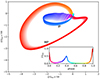 |
Fig. 8. Stokes parameters Q and U for the pulsar alone, extracted from the phenomenological model fit to IXPE data, without phase shifts in the polarization angle. The color gradient corresponds to the pulse phase, as shown in the subplot for the pulse profile (observed by Chandra). The transparency gradient corresponds to different DC subtractions from the optical Stokes, ranging from 0% subtraction for the most transparent curve to 90% subtraction for the least transparent curve (correspondingly, β/α ranges from 0.46 to 0.56; see Section 3 for more details). |
In the presence of vacuum birefrigence, a highly magnetized and fast-rotation pulsar may produce a phase shift in the polarization angle between different bands, for instance, with the polarization angle swing in the optical band lagging the X-ray band. The strong phase shifts at the interpulse for the first two IXPE observations are probably not associated with the vacuum birefringence, as they are higher by about one order of magnitude than early theoretical calculations, which predicted values in the range δ ≈ 1 − 2% for a corrotating dipole model or Deutsch model (Heyl & Shaviv 2000). Instead, our results suggest some form of variability in the polarization angle swing at the interpulse, as observed when analyzing each IXPE observation separately. The origin of this variability is unknown. A theoretical study of this phenomenon is beyond the scope of this paper and is left for future work.
Nevertheless, in addition to producing phase shifts in the polarization angle, vacuum birefringence primarily causes the polarization modes of the photons to readapt to the local magnetic field as radiation propagates through the magnetosphere. This effect takes place up to the polarization limiting radius, which is located at several tens of NS radii; beyond this, the magnetic field weakens and the photon polarization mode freezes (Heyl & Shaviv 2002). The nondetection of a (positive) phase shift at the main pulse in all three IXPE observations likely indicates that the emission mechanism takes place beyond the polarization limiting radius, perhaps outside the light cylinder, as discussed in several current sheet models/simulations of pulsar magnetosphere (see e.g., Pétri & Kirk 2005; Contopoulos & Kalapotharakos 2010; Cerutti et al. 2016; Harding & Kalapotharakos 2017). On the other hand, the variability of the phase shift at the interpulse suggests that the emission mechanism might be located in regions where the pulsar magnetosphere might undergo through some form of rearrangement on timescales comparable to the timescale between different IXPE observations. However, this scenario contradicts the X-ray pulse profile of the Crab pulsar, which has been studied for many years and shows no variability at the interpulse. If the variability of the polarization angle swing at the interpulse is confirmed by future polarization observations, it would suggest some form of decoupling between the flux and formation of the polarization angle. The origin of this phenomenon will pose a new challenge for theoretical studies of pulsar emission and polarization.
In addition, another consequence of the vacuum birefringence is that at the polarization limiting radius, the polarization modes of the radiation align with the more uniform projected magnetic field on the plane in the sky, as well as with the projected magnetic axis (Heyl & Shaviv 2002). As the pulsar rotates, the phase-dependent polarization angle is therefore expected to follow a simple rotating vector model (Radhakrishnan & Cooke 1969; González-Caniulef et al. 2023). However, the Crab pulsar behaves differently. It deviates from the rotation vector model in the optical and X-rays polarimetric observations. This deviation again indicates that the emission mechanisms for the main pulse and interpulse are likely produced beyond the polarization limiting radius and remain unaffected by the vacuum birefringence.
If the X-ray emission indeed takes place far away in the magnetosphere, its reduced polarization compared to the optical band might indicate that these emissions originate from different regions. Specifically, while the X-rays might be produced close to the light cylinder radius, where turbulence due to reconnection at the Y-point might be stronger and the level of polarization is accordingly relatively low, the optical emission might be located farther out, in the striped wind, where turbulence might have decayed, allowing for a higher degree of polarization. For emission located at or beyond the light cylinder, the expected phase lag due to the different location of the emitting region is typically very small (Pétri 2013). This demonstrates that X-ray polarization information may serve to probe pulsar magnetospheres and potentially the current sheet scenario that was discussed in particle-in-cell simulations (for a recent review see e.g., Philippov & Kramer 2022).
Our results pave the way for a systematic search via optical and X-ray polarimetric observations for phase shifts in sources similar to the Crab pulsar, and for gaining insight into the emission mechanism. In particular, PSR B0540+69 is a promising source. Located in the Large Magellanic Cloud, it is considered the “Crab twin”. This source shows phase-aligned light curves from radio to gamma rays, as well as dominant nonthermal emission in the optical and X-rays. Polarimetric observations with HST/WFP detected phase-averaged PD = 16 ± 4% and PA = 22° ±12° (Mignani et al. 2010). Recent IXPE observations for a phase-dependent analysis revealed two bins with PD of 68 ± 20% and 62 ± 20% (Xie et al. 2024). Further polarimetric observations in the optical and X-ray bands are needed to verify whether common phase-dependent polarization properties are present in this source as well.
Expanding the comparison to include gamma-ray observations of the Crab should also be a key objective for future research (see e.g., Dean et al. 2008; Li et al. 2022).
These phase shifts may also be investigated, for example, in the phase bins in which polarization was detected, as reported in Wong et al. (2024). However, as we show below, our fit uses all phase bins at a time, which makes it more sensitive to the detection of phase shifts if the model is acceptable.
For a dipolar magnetic field, the polarization limiting radius is defined as  , where μ is the magnetic dipole moment of the NS, ν is the frequency of the radiation, and θ is the angle between the magnetic axis and the line of sight (Heyl & Shaviv 2002).
The interpulse is also energy dependent, and the ratio of the intensity of the main pulse to the interpulse is lower in the X-rays than in the optical.
The α parameter also absorbs missing instrumental effects in the transformation of the unfolded and unabsorved intensity from the Chandra to the IXPE folded intensity, which explains why the values of α/Δt listed in Table 1 are not exactly one.
The radio light curve is significantly different from the curves in the optical/X-rays.
MDP is the minimum detectable polarization at the 99% confidence level, where μ is the modulation factor of the detector, and N is the number of counts (when the background is negligible).
By combining all three observations, it is not possible to obtain a unique measurement of the phase shift at the interpulse as the associated posterior distribution shows multiple peaks.
From the probability density function for the χ2 distribution, we obtain that the odds ratio of the models with and without the phase shifts is ≈2.
Acknowledgments
We thank the referee for their constructive comments. We also thank Benjamin Crinquand for discussions that benefited this paper. DGC acknowledges support from a CNES fellowship. JH acknowledges support from the Natural Sciences and Engineering Research Council of Canada (NSERC) through a Discovery Grant and the Canadian Space Agency through the co-investigator grant program. NB was supported by the INAF MiniGrant “PWNnumpol – Numerical Studies of Pulsar Wind Nebulae in The Light of IXPE”. F.X. is supported by National Natural Science Foundation of China (grant No. 12373041), and special funding for Guangxi distinguished professors (Bagui Xuezhe). This work is partially supported by MAECI with grant CN24GR08 “GRBAXP: Guangxi-Rome Bilateral Agreement for X-ray Polarimetry in Astrophysics”. This research was enabled in part by support provided by Compute Canada (www.computecanada.ca), UBC ARC Sockeye infrastructure, and the SciServer science platform (www.sciserver.org).
References
- Baldini, L., Bucciantini, N., Lalla, N. D., et al. 2022, SoftwareX, 19, 101194 [NASA ADS] [CrossRef] [Google Scholar]
- Bucciantini, N., Ferrazzoli, R., Bachetti, M., et al. 2023, Nat. Astron., 7, 602 [NASA ADS] [CrossRef] [Google Scholar]
- Bucciantini, N., Romani, R. W., Xie, F., & Wong, J. 2024, Galaxies, 12, 45 [NASA ADS] [CrossRef] [Google Scholar]
- Bühler, R., & Blandford, R. 2014, Rep. Progr. Phys., 77, 066901 [CrossRef] [Google Scholar]
- Cerutti, B., Mortier, J., & Philippov, A. A. 2016, MNRAS, 463, L89 [NASA ADS] [CrossRef] [Google Scholar]
- Chauvin, M., Roques, J. P., Clark, D. J., & Jourdain, E. 2013, ApJ, 769, 137 [NASA ADS] [CrossRef] [Google Scholar]
- Chauvin, M., Florén, H. G., Friis, M., et al. 2017, Sci. Rep., 7, 7816 [NASA ADS] [CrossRef] [Google Scholar]
- Cocke, W. J., Disney, M. J., & Gehrels, T. 1969, Nature, 223, 576 [CrossRef] [Google Scholar]
- Contopoulos, I., & Kalapotharakos, C. 2010, MNRAS, 404, 767 [Google Scholar]
- Dean, A. J., Clark, D. J., Stephen, J. B., et al. 2008, Science, 321, 1183 [NASA ADS] [CrossRef] [Google Scholar]
- Feng, H., Li, H., Long, X., et al. 2020, Nat. Astron., 4, 511 [CrossRef] [Google Scholar]
- Foreman-Mackey, D., Hogg, D. W., Lang, D., & Goodman, J. 2013, PASP, 125, 306 [Google Scholar]
- Forot, M., Laurent, P., Grenier, I. A., Gouiffès, C., & Lebrun, F. 2008, ApJ, 688, L29 [NASA ADS] [CrossRef] [Google Scholar]
- Goldreich, P., & Julian, W. H. 1969, ApJ, 157, 869 [Google Scholar]
- González-Caniulef, D., Caiazzo, I., & Heyl, J. 2023, MNRAS, 519, 5902 [CrossRef] [Google Scholar]
- Harding, A. K. 2019, Astrophys. Space Sci. Lib., 460, 277 [NASA ADS] [CrossRef] [Google Scholar]
- Harding, A. K., & Kalapotharakos, C. 2017, ApJ, 840, 73 [NASA ADS] [CrossRef] [Google Scholar]
- Harding, A. K., Venter, C., & Kalapotharakos, C. 2021, ApJ, 923, 194 [Google Scholar]
- Heisenberg, W., & Euler, H. 1936, Z. Phys., 98, 714 [NASA ADS] [CrossRef] [Google Scholar]
- Heyl, J. S., & Shaviv, N. J. 2000, MNRAS, 311, 555 [NASA ADS] [CrossRef] [Google Scholar]
- Heyl, J. S., & Shaviv, N. J. 2002, Phys. Rev. D, 66, 023002 [NASA ADS] [CrossRef] [Google Scholar]
- Heyl, J., González-Caniulef, D., & Caiazzo, I. 2024, Open J. Astrophys., 7, 35 [NASA ADS] [CrossRef] [Google Scholar]
- Kristian, J., Visvanathan, N., Westphal, J. A., & Snellen, G. H. 1970, ApJ, 162, 475 [NASA ADS] [CrossRef] [Google Scholar]
- Li, H.-C., Produit, N., Zhang, S.-N., et al. 2022, MNRAS, 512, 2827 [NASA ADS] [CrossRef] [Google Scholar]
- Long, X., Feng, H., Li, H., et al. 2021, ApJ, 912, L28 [NASA ADS] [CrossRef] [Google Scholar]
- Marshall, H. L. 2021, AJ, 162, 134 [NASA ADS] [CrossRef] [Google Scholar]
- Mignani, R. P. 2018, Galaxies, 6, 36 [NASA ADS] [CrossRef] [Google Scholar]
- Mignani, R. P., Sartori, A., de Luca, A., et al. 2010, A&A, 515, A110 [NASA ADS] [CrossRef] [EDP Sciences] [Google Scholar]
- Mignani, R. P., Testa, V., González Caniulef, D., et al. 2017, MNRAS, 465, 492 [NASA ADS] [CrossRef] [Google Scholar]
- Moran, P., Shearer, A., Mignani, R. P., et al. 2013, MNRAS, 433, 2564 [NASA ADS] [CrossRef] [Google Scholar]
- Pétri, J. 2013, MNRAS, 434, 2636 [CrossRef] [Google Scholar]
- Pétri, J., & Kirk, J. G. 2005, ApJ, 627, L37 [CrossRef] [Google Scholar]
- Philippov, A., & Kramer, M. 2022, ARA&A, 60, 495 [NASA ADS] [CrossRef] [Google Scholar]
- Radhakrishnan, V., & Cooke, D. J. 1969, Astrophys. Lett., 3, 225 [NASA ADS] [Google Scholar]
- Schwinger, J. 1951, Phys. Rev., 82, 664 [NASA ADS] [CrossRef] [Google Scholar]
- Słowikowska, A., Kanbach, G., Kramer, M., & Stefanescu, A. 2009, MNRAS, 397, 103 [CrossRef] [Google Scholar]
- Smith, F. G., Jones, D. H. P., Dick, J. S. B., & Pike, C. D. 1988, MNRAS, 233, 305 [NASA ADS] [CrossRef] [Google Scholar]
- Trimble, V. 1973, PASP, 85, 579 [NASA ADS] [CrossRef] [Google Scholar]
- Vadawale, S. V., Chattopadhyay, T., Mithun, N. P. S., et al. 2018, Nat. Astron., 2, 50 [Google Scholar]
- Weisskopf, V. 1936, Kong. Dan. Vid. Sel. Mat. Fys. Med., 14N6, 1 [NASA ADS] [Google Scholar]
- Weisskopf, M. C., Silver, E. H., Kestenbaum, H. L., Long, K. S., & Novick, R. 1978, ApJ, 220, L117 [NASA ADS] [CrossRef] [Google Scholar]
- Weisskopf, M. C., Tennant, A. F., Yakovlev, D. G., et al. 2011, ApJ, 743, 139 [Google Scholar]
- Weisskopf, M. C., Soffitta, P., Baldini, L., et al. 2022, J. Astron. Telesc. Instrum. Syst., 8, 026002 [NASA ADS] [CrossRef] [Google Scholar]
- Wilms, J., Allen, A., & McCray, R. 2000, ApJ, 542, 914 [Google Scholar]
- Wong, J., Romani, R. W., & Dinsmore, J. T. 2023, ApJ, 953, 28 [NASA ADS] [CrossRef] [Google Scholar]
- Wong, J., Mizuno, T., Bucciantini, N., et al. 2024, ApJ, 973, 172 [NASA ADS] [CrossRef] [Google Scholar]
- Xie, F., Wong, J., La Monaca, F., et al. 2024, ApJ, 962, 92 [NASA ADS] [CrossRef] [Google Scholar]
Appendix A: Optical Stokes
Figure A.1 shows the Stokes parameters in the optical band (IV, QV, UV), which are taken from Słowikowska et al. (2009) and smoothed with a Radial basis function interpolation. The interpulse and main peaks are located at 0.396 and 0.993 in phase, respectively, relative to the radio peak.
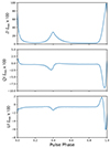 |
Fig. A.1. Optical Stokes parameters for Crab pulsar (IV, QV, UV). |
Appendix B: Intensity from Chandra X-ray observations
Figure B.1 shows the soft X-ray spectrum of Crab pulsar used to model ICX, based on Chandra observations from Weisskopf et al. (2011), which is parameterized as a power law whose normalization and index vary in phase. The spectral index as a function of the pulse phase has been fitted to a sinusoidal in order to have a sufficiently smooth pulse profile. The interpulse and main peaks are located at 0.393 and 0.990 in phase, respectively, relative to the radio peak.
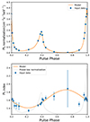 |
Fig. B.1. Power-law normalization and index for the phase-dependent spectrum of Crab pulsar in soft X-rays. Data points (in blue) are taken from Weisskopf et al. (2011). The orange curve in the first and second panel correspond to a spline interpolation and a sinusoidal fit, respectively. |
Appendix C: Fits for the three observations of Crab Pulsar by IXPE
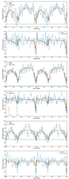 |
Fig. C.1. All three IXPE observation of Crab pulsar and the best fitted polarimetric model (subtracting 90% of DC component to the Stokes parameters in the optical band). The first (second), third (fourth) and fifth (sixth) panels correspond to the polarization degree (polarization angle) for the first, second, and third observation of crab pulsar, respectively. The green line corresponds to MDP99. The gray solid lines correspond to the best-fitted model without phase shift. The orange and gray arrows in the fourth panel highlight the polarization angle swing, at the interpulse, with and without a phase shift, respectively. |
All Tables
Summary of the model parameters we fit to three separate observations of the Crab pulsar by IXPE.
All Figures
|
Fig. 1. Phenomenological polarization angle model, φX, for the pulsar in the X-rays considering positive and negative phase shifts from −5% to 5% at the interpulse (upper panel) and main pulse (lower panel). For reference, the dotted black line shows the optical (V-band) polarization angle, and the solid red curve shows the I Stokes (V-band, with arbitrary normalization) from Słowikowska et al. (2009). The phase shifts are applied within the boundaries indicated by the vertical dashed blue lines. |
| In the text | |
|
Fig. 2. Best-fit model to the first observation of the Crab pulsar by IXPE in the 2 − 4 keV range. The data reduction was performed with the IXPEOBSSIM package considering equipopulated binning for the Stokes parameters (first panel), and for the polarization degree (second panel) and polarization angle (third panel). The green line in the second panel corresponds to MDP99. The solid gray lines in the first three panels correspond to the best-fit model without a phase shift. The orange and gray arrows highlight the polarization angle swing at the interpulse with and without a phase shift, respectively. For completeness, we include the pulse profile with 400 equispaced bins (fourth panel). |
| In the text | |
|
Fig. 3. Posterior distributions for the first observation of the Crab pulsar by IXPE. The model parameters include the phase shifts at the main pulse (δP) and interpulse (δI). The MCMC analysis was performed using 100 walkers and 10 000 steps. The blue lines show the solution obtained with a minimization routine. |
| In the text | |
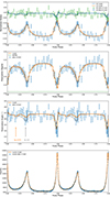 |
Fig. 4. Same as Figure 2 for the second observation of the Crab pulsar by IXPE. |
| In the text | |
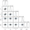 |
Fig. 5. Same as Figure 3 for the second IXPE observation of the Crab pulsar. |
| In the text | |
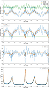 |
Fig. 6. Same as Figure 2 for the third observation of the Crab pulsar by IXPE. |
| In the text | |
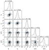 |
Fig. 7. Same as Figure 3 for the third observation of the Crab pulsar by IXPE. |
| In the text | |
|
Fig. 8. Stokes parameters Q and U for the pulsar alone, extracted from the phenomenological model fit to IXPE data, without phase shifts in the polarization angle. The color gradient corresponds to the pulse phase, as shown in the subplot for the pulse profile (observed by Chandra). The transparency gradient corresponds to different DC subtractions from the optical Stokes, ranging from 0% subtraction for the most transparent curve to 90% subtraction for the least transparent curve (correspondingly, β/α ranges from 0.46 to 0.56; see Section 3 for more details). |
| In the text | |
|
Fig. A.1. Optical Stokes parameters for Crab pulsar (IV, QV, UV). |
| In the text | |
|
Fig. B.1. Power-law normalization and index for the phase-dependent spectrum of Crab pulsar in soft X-rays. Data points (in blue) are taken from Weisskopf et al. (2011). The orange curve in the first and second panel correspond to a spline interpolation and a sinusoidal fit, respectively. |
| In the text | |
|
Fig. C.1. All three IXPE observation of Crab pulsar and the best fitted polarimetric model (subtracting 90% of DC component to the Stokes parameters in the optical band). The first (second), third (fourth) and fifth (sixth) panels correspond to the polarization degree (polarization angle) for the first, second, and third observation of crab pulsar, respectively. The green line corresponds to MDP99. The gray solid lines correspond to the best-fitted model without phase shift. The orange and gray arrows in the fourth panel highlight the polarization angle swing, at the interpulse, with and without a phase shift, respectively. |
| In the text | |
Current usage metrics show cumulative count of Article Views (full-text article views including HTML views, PDF and ePub downloads, according to the available data) and Abstracts Views on Vision4Press platform.
Data correspond to usage on the plateform after 2015. The current usage metrics is available 48-96 hours after online publication and is updated daily on week days.
Initial download of the metrics may take a while.