| Issue |
A&A
Volume 689, September 2024
|
|
|---|---|---|
| Article Number | A200 | |
| Number of page(s) | 9 | |
| Section | Extragalactic astronomy | |
| DOI | https://doi.org/10.1051/0004-6361/202451037 | |
| Published online | 13 September 2024 | |
Testing particle acceleration in blazar jets with continuous high-cadence optical polarization observations
1
Institute of Astrophysics, Foundation for Research and Technology-Hellas, 70013
Heraklion, Greece
2
NASA Marshall Space Flight Center, Huntsville, AL, 35812
USA
3
Department of Physics, University of Crete, 70013
Heraklion, Greece
4
Institute for Astrophysical Research, Boston University, 725 Commonwealth Avenue, Boston, MA, 02215
USA
5
University of Maryland Baltimore, County Baltimore, MD, 21250
USA
6
NASA Goddard Space Flight Center Greenbelt, MD, 20771
USA
7
Saint Petersburg State University, 7/9 Universitetskaya nab., St., Petersburg, 199034
Russia
8
Instituto de Astrofísica de Andalucía, IAA-CSIC, Glorieta de la Astronomía s/n, 18008
Granada, Spain
9
Instituto de Astronomía, Universidad Nacional Autónoma de México, A.P. 70-264, CDMX 04510, México, Ensenada 22800, Baja California, Mexico
10
Department of Physics and Astronomy, University of Turku, 20014
Finland
11
INAF Osservatorio Astronomico di Brera, Via E. Bianchi 46, 23807
Merate (LC), Italy
12
Institute of Astronomy, National Central University, Taoyuan, 32001
Taiwan
13
Department of Physics, Graduate School of Advanced Science and Engineering, Hiroshima University Kagamiyama, 1-3-1 Higashi-Hiroshima, Hiroshima, 739-8526
Japan
14
Astrophysics Research Institute, Liverpool John Moores University, Liverpool Science Park IC2, 146 Brownlow Hill, Liverpool, L3 5RF
UK
15
Finnish Centre for Astronomy with ESO (FINCA), FI-20014
University of Turku, Finland
16
Facultad de Ciencias, Universidad Autónoma de Baja California, Campus El Sauzal, 22800
Ensenada, Baja California, Mexico
17
Aryabhatta Research Institute of Observational Sciences (ARIES), Manora Peak, Nainital, 263002
India
18
Center for Basic Sciences, Pt. Ravishankar Shukla University, Raipur, Chhattisgarh, 492010
India
19
Department of Applied Physics/Physics, M.J.P. Rohilkhand University, Bareilly, Uttar Pradesh, 24300
India
20
Institute of Innovative Research (IIR), Tokyo Institute of Technology, 2-12-1 Ookayama, Meguro-ku, Tokyo, 152-8551
Japan
21
Pulkovo Observatory, St.Petersburg, 196140
Russia
22
Special Astrophysical Observatory of Russian Academy of Sciences, Nizhnij Arkhyz, Karachai-Cherkessian Republic, 369167
Russia
23
Instituto de Estudios Astrofísicos, Facultad de Ingeniería y Ciencias, Universidad Diego Portales, Santiago Región Metropolitana, 8370191
Chile
24
Steward Observatory, University of Arizona, 933 North Cherry Avenue, Tucson
AZ, 85721-0065
USA
25
Hiroshima Astrophysical Science Center, Hiroshima University 1-3-1 Kagamiyama, Higashi-Hiroshima, Hiroshima, 739-8526
Japan
26
Core Research for Energetic Universe (Core-U), Hiroshima University, 1-3-1 Kagamiyama, Higashi-Hiroshima, Hiroshima, 739-8526
Japan
27
Centre for Astrophysics Research, University of Hertfordshire, Hatfield, AL10 9AB
UK
28
School of Physics and Astronomy, University of Leicester, University Road, Leicester, LE1 7RH
UK
Received:
8
June
2024
Accepted:
21
June
2024
Abstract
Variability can be the pathway to understanding the physical processes in astrophysical jets. However, the high-cadence observations required to test particle acceleration models are still missing. Here we report on the first attempt to produce continuous, > 24 hour polarization light curves of blazars using telescopes distributed across the globe, following the rotation of the Earth, to avoid the rising Sun. Our campaign involved 16 telescopes in Asia, Europe, and North America. We observed BL Lacertae and CGRaBS J0211+1051 for a combined 685 telescope hours. We find large variations in the polarization degree and angle for both sources on sub-hour timescales as well as a ∼180° rotation of the polarization angle in CGRaBS J0211+1051 in less than two days. We compared our high-cadence observations to particle-in-cell magnetic reconnection and turbulent plasma simulations. We find that although the state-of-the-art simulation frameworks can produce a large fraction of the polarization properties, they do not account for the entirety of the observed polarization behavior in blazar jets.
Key words: radiation mechanisms: non-thermal / techniques: polarimetric / galaxies: active / BL Lacertae objects: general / galaxies: jets
Corresponding authors; This email address is being protected from spambots. You need JavaScript enabled to view it. .
© The Authors 2024
 Open Access article, published by EDP Sciences, under the terms of the Creative Commons Attribution License (https://creativecommons.org/licenses/by/4.0), which permits unrestricted use, distribution, and reproduction in any medium, provided the original work is properly cited.
This article is published in open access under the Subscribe to Open model. This email address is being protected from spambots. You need JavaScript enabled to view it. to support open access publication.
1. Introduction
Blazars are active galactic nuclei with powerful jets oriented within a few degrees of the line of sight of an observer on Earth (Blandford et al. 2019; Hovatta & Lindfors 2019). They show a plethora of exciting behavior, but are most notable for their broadband emission from radio to γ-rays (e.g., Ajello et al. 2020), extreme variability down to minute timescales (e.g., Ackermann et al. 2016), highly polarized emission, with a polarization degree that can exceed 45% (e.g., Shao et al. 2019), and highly relativistic jets (Lister et al. 2021; Weaver et al. 2022). The origin of the extreme, diverse variability in different wavelengths is not fully understood but holds the keys to understanding the physical processes in astrophysical jets. A few models have now been proposed to explain the observed variability patterns. They include shocks in jets (Marscher & Gear 1985), jets in jets (Giannios et al. 2009), turbulence (Marscher 2014; Webb & Sanz 2023), magnetic reconnection (Hosking & Sironi 2020; Zhang et al. 2020), shock-shock collisions (Liodakis et al. 2020), kink instabilities (Zhang et al. 2017), Doppler factor variations (Raiteri et al. 2017b,a), and others. A great deal of effort has been made to characterize the jet’s variability on diverse timescales. The recent introduction of datasets from exoplanet satellites like Kepler and the Transiting Exoplanets Survey Satellite (TESS) (Sasada et al. 2017; Weaver et al. 2020; Raiteri et al. 2021) has given us an additional unique view of blazar variability. However, despite all these efforts, we still lack a consensus on the mechanisms that drive variability in blazar jets.
Polarization can also be used to probe the physical processes that govern the jets. This is because different models often predict different polarization properties (e.g., Marscher 2014; Zhang et al. 2014; Peirson & Romani 2018, 2019; Tavecchio 2021). Moreover, blazars show a peculiar polarization behavior that often takes place in the form of rotations of the polarization angle (e.g., Marscher et al. 2008, 2010; Blinov et al. 2015, 2016a). Polarization studies of blazars have been limited by the cadence of the observations, the lack of dedicated experiments (see Kiehlmann et al. 2021 for a discussion), and, until recently, the limited wavelength coverage, as most studies had been in the optical. The recent launch of the Imaging X-ray Polarimetry Explorer (IXPE; Weisskopf et al. 2022) has opened new avenues to studying the high-energy Universe. The first observations of blazars suggest that particle acceleration in jets takes place in shocks, with the emission becoming energy-stratified owing to particle cooling (Liodakis et al. 2022; Di Gesu et al. 2022; Kouch et al. 2024). More interestingly, IXPE has already managed to detect the first X-ray polarization angle rotation in Mrk 421 (Di Gesu et al. 2023; Kim et al. 2024) in a blind survey. Mrk 421 showed a > 360° rotation with a rate of 80–90° d−1. This would suggest that large variations in the polarization angle can take place within a single observing night (see also MAGIC Collaboration 2018) and are missed in the optical because of the 180° ambiguity of the polarization angle and our inability to monitor a blazar from one location continuously. Uninterrupted observations have only been achieved in a limited number of campaigns (e.g., Bhatta et al. 2016; Weaver et al. 2020).
Here we aim to combine the power of variability and polarization by producing continuous light curves from ground-based observations. This was achieved by combining multiple telescopes across the world using the rotation of the Earth. Different telescopes have often been combined for blazar studies (e.g., Raiteri & Villata 2021) and other purposes (e.g., Brown et al. 2013). Here we focus on polarimetry and probing shorter variability timescales by producing continuous, uninterrupted, longer than 24-hour time series that we can use to test particle acceleration models. In Sect. 2 we describe the telescopes used in this work and our observing strategy, and in Sect. 3 we discuss our analysis procedures. In Sect. 4 we present the final time series and examine their variability properties. In Sect. 5 we test different models of particle acceleration, and in Sect. 6 we discuss our findings. We focus on linear polarization, which we refer to as “polarization” throughout the paper for simplicity.
2. Telescopes and observing strategy
Our campaign, which we dubbed the NOn-stop Polarization Experiment (NOPE), consisted of 16 telescopes across the world with a combined 685 telescope hours over seven nights. Those telescopes/observatories are, the Aryabhatta Research Institute of Observational Sciences (ARIES), the Calar Alto Observatory, the Crimean Observatory, T60 at the Haleakala Observatory (Piirola et al. 2014, 2020), the Kanata telescope (Uemura et al. 2017), the Liverpool Telescope (Steele et al. 2004), LX-200 (Larionov et al. 2008), Lulin Observatory, the Nordic Optical Telescope (Hovatta et al. 2016; Nilsson et al. 2018), the Perkins Telescope Observatory (PTO; Jorstad et al. 2010), the Observatorio Astronómico Nacional at San Pedro Mártir (OAN-SPM), the Zeiss-1000/MAGIC at the Special Astrophysical Observatory of RAS (Afanasiev et al. 2023; Komarov et al. 2020), Sierra Nevada Observatory, RoboPol at the Skinakas Observatory (Ramaprakash et al. 2019), and the University of Leicester Observatory (Wiersema et al. 2023). NOPE was scheduled for the dark time of 2–8 November 2021. The volcano eruption in La Palma prevented us from acquiring data from the Liverpool Telescope and the Nordic Optical Telescope. Weather related reasons prevented the use of the telescope at the University of Leicester Observatory as well. Additional telescope hours were lost due to weather in different locations; however, all remaining telescopes provided a reasonable amount of data.
To probe fast variability timescales, we selected the most variable sources found from the four years of monitoring in the RoboPol sample (Blinov et al. 2021) that were visible for at least half the night from most locations. Since rotations of the polarization has been shown to be connected to γ-ray activity (Blinov et al. 2018), we monitored the γ-ray light curves of all the objects in the sample (Baldini et al. 2021; Abdollahi et al. 2023) as well as for other flaring sources using alert brokers (e.g., Astronomer’s telegram1).
3. Optical polarization observations
3.1. Observations and data reduction
At the time of the scheduled observations, there were no outbursts or elevated activity reported; hence, we opted to observe BL Lacertae (BL Lac), which was in a prolonged outburst that had lasted a few months (Raiteri et al. 2023) and CGRaBS J0211+1051 (hereafter J0211) that was in a historically low brightness and low polarization degree period (Blinov et al. 2021). BL Lac is typically a low synchrotron peaked blazar (i.e., synchrotron peak frequency < 1014 Hz, Ajello et al. 2020; Middei et al. 2023), but turns into an intermediate peaked source during flares (i.e., synchrotron peak frequency 1014 < νsyn < 1015 Hz; e.g., Peirson et al. 2023). J0211 is an intermediate peaked blazar (Peirson et al. 2022). BL Lac was observed for the first half of each night while J0211 for the second half. The observations were performed in the R band. The data were analyzed using either standard analysis procedures or existing pipelines at individual observatories (e.g., King et al. 2014; Panopoulou et al. 2015; Nilsson et al. 2018). All the polarimetric measurements were performed with a 5″ aperture radius. We preselected several polarized (HD 204827 and BD +59.389) and unpolarized (BD+32.3739, BD +28.4211, HD 212311, HD 14069, and G191B2B) standard stars, commonly used by blazar monitoring program like the Steward Observatory2 and RoboPol (Blinov et al. 2023), to be used by all the observatories. Since we are interested in the polarization variability, we did not apply any correction to the polarization degree from the dilution of the host-galaxy, which, at the selected aperture, should be negligible (e.g., Meisner & Romani 2010).
For both sources we are able to achieve a median cadence of five minutes. The shortest interval between observations was zero, and the longest, which occurred toward the end of our campaign, was roughly nine hours for BL Lac and twelve hours for J0211.
3.2. Data post-processing
Systematic shifts. Once all the data were collected, small systematic shifts on the order of < 0.1mag and < 0.5% were applied to the brightness and polarization degree, respectively, to align overlapping observations. Those shifts originate from the different efficiency in the instruments, instrumental setup, seeing, and minor differences in the analysis pipelines.
Data binning. We averaged data points in bins of 30 min duration. These bins were interactively identified3 using the method described in Kiehlmann (2015, Sect. 2.1.2). In the selected bins, we calculated the mean value of q and u. Even though the variability in the bins is below the noise level, we expected some intrinsic variability. Therefore, we did not use the uncertainty-weighted mean, which is based on the assumption that all measurements are estimates of the same intrinsic value. To derive realistic uncertainties for the average q and u, we calculated (i) the mean of the corresponding uncertainties and (ii) the standard deviation of q and u in the bin, and we used the larger value of the two. We then calculated the corresponding p and χ using Eq. (1),
 (1)
(1)
and we used the procedure described in Blinov et al. (2021) to estimate the corresponding uncertainties. We corrected for the ±180° ambiguity of the polarization angle following Kiehlmann et al. (2016). The brightness and polarization light curves for both sources used in the paper are available at the Harvard Dataverse (Liodakis 2024)4.
4. Variability properties
4.1. Light curves
Figures 1 and 2 show the observations for BL Lac and J0211, respectively. BL Lac shows rapid intra-night flaring that would be impossible to fully characterize with observations of less than 12 hours. The R-band magnitude of the source varies from a minimum of 12.87mag to a maximum of 12.15mag, with a median of 12.48mag and ∼0.5mag flares. The polarization degree (Π) has a min and max of 7.3% and 18.9%, respectively, with a median of 11.7%. The polarization angle (ψ) remains near the jet axis on the sky (10° ± 2°; Weaver et al. 2022), fluctuating from 12° to 39° with a median of 25°. There is no correlation between brightness and polarization as is typical of blazars (Ikejiri et al. 2011; Blinov et al. 2016b; Jermak et al. 2016).
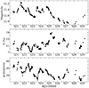 |
Fig. 1. NOPE observations of BL Lac. The top panel shows the R-band magnitude, the middle panel the polarization degree, and the bottom panel the polarization angle. The observations have been grouped into 30 min bins (see the main text). |
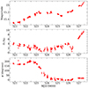 |
Fig. 2. NOPE observations of CGRaBS J0211+1051. The top panel shows the R-band magnitude, the middle panel the polarization degree, and the bottom panel the polarization angle. The observations have been grouped into 30 min bins (see the main text). |
J0211 exhibits a more complex behavior with smoother variations than BL Lac. The R-band magnitude ranges from 15.5mag to 14.9mag with a median of 15.2mag. Π ranges from 0.43% to 9.3% with a median of 2.7%. We observe both a correlation and anticorrelation between brightness and the polarization degree. At the start of our campaign, J0211 shows a smooth increase in brightness. At the same time Π decreases from about 5% to the lowest observed value of 0.43%, which occurs at peak brightness. Then the polarization degree starts to recover. During the increase in brightness and drop of Π we observe a smooth monotonic 185° rotation of the ψ from ∼200° to ∼15°. Figure 3 shows the progression of the rotation in the Q–U plane. There is a clear circular motion of the Stokes vectors indicating the presence of a rotation slightly offset from 0–0. The jet direction has been determined at 15 GHz to be 88° ±9° (Hodge et al. 2018), which suggests that the rotation started and ended roughly perpendicular to the jet. The drop of Π during ψ rotations in the optical is a common feature in the blazar population (Blinov et al. 2016b). After the rotation, ψ remains constant while the brightness and Π show a clear correlation.
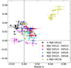 |
Fig. 3. Stokes Q versus Stokes U for CGRaBS J0211+1051. The data have been divided according to the MJD to show the progression of the rotation in the Q–U plane. The dashed black lines mark 0–0. |
4.2. Bayesian block analysis
We used Bayesian block (BB) analysis (Scargle et al. 2013) to model the brightness and polarization degree light curves (e.g., Liodakis et al. 2018, 2019b). BB analysis has only one parameter, ncrprior, which is related to the prior for the number of bins. Following de Jaeger et al. (2023), we used a value of the ncrprior that yields a false-positive rate (p0) of p0 = 0.01. We also implemented the HOP module (Eisenstein & Hut 1998; Meyer et al. 2019) that allows us to trace changes in the block flux derivative. That allows us to separate extended time intervals that could be considered as flares or parts of a flare. For the brightness, we converted the R-band magnitudes to flux density in mJy using F = 10(6.489 − 0.4 × mag), as suggested by Mead et al. (1990). For both the flux density and Π, we estimated the amplitude of the variations by subtracting the value of the lowest BB over the entire dataset, and used the width of the BBs as a proxy for the variability timescale.
Figures 4 and 5 show the BB analysis for the flux density and Π, respectively. For BL Lac, we find similar variability timescales, on average, for both the flux density and Π. The average timescale is about 4 h, with a minimum and maximum of 0.9 and ∼24 h, respectively. Π shows more peaks with amplitudes that vary between 3.3% and 10.6% with an average of 5%. The brightness shows four peaks of similar amplitude that range from 13.2 to 19.3 mJy. For the brightness and the Π, the average flaring period is 24 and 25.5 h, respectively, with a minimum of 16.6 and 18.5 h. These are comparable to the timescales for optical and X-rays (15 and 14.5 h, respectively) found in Weaver et al. (2020).
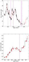 |
Fig. 4. BB representation (dashed line) of the flux density variations of BL Lac (top panel) and CGRaBS J0211+1051 (bottom panel). The vertical magenta lines show the edges of the time intervals identified by the HOP module. |
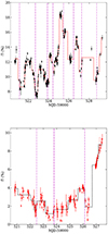 |
Fig. 5. BB representation (dashed line) of the polarization degree variations of BL Lac (top panel) and CGRaBS J0211+1051 (bottom panel). The vertical magenta lines show the edges of the time intervals identified by the HOP module. |
For J0211 there is a single peak in brightness and two small-amplitude flares in Π. There is a clear rise in both at the end of our campaign; we unfortunately were not able to capture the peak. The amplitude of the peak in brightness is 0.57 mJy and in Π is 2.5%. The average variability timescale is 11.7 h for brightness and 13.3 h for Π. The minimum and maximum are 3.5 and 23.8 h for brightness and 3 and 34.2 h for the degree of polarization, respectively. The duration of the flaring period for the brightness is 75.6 h and for Π 31.6 and 55.7 h, respectively. Table 1 summarizes the results from the BB analysis.
BB analysis.
5. Testing particle acceleration models
The temporal behavior of the flux and polarization of both BL Lac and J0211+1051 gives the impression that stochastic processes play an important role in driving the variations. This is especially apparent in BL Lac, in which there is ∼1 reversal per day in the time derivative of the flux, and ∼2 reversals per day in both polarization degree and angle. To understand the origin of such short-term variability, we employed two distinct numerical models that involve stochastic physical processes: magnetic reconnection modeled by particle-in-cell (PIC) simulations and a scenario in which turbulent plasma crosses a shock. We also tested a scenario were both processes contribute equally to the emission. In this section we present the outcomes of numerical computations based on these models, and contrast the results with the observational data. J0211 exhibits much smoother behavior with only a small number of features. Therefore, we concentrated on BL Lac since the NOPE observations sample a large number of reversals of the time derivatives of these observed quantities, and thus provide sufficient statistics to test the ability of the models to reproduce the essence of the observed behavior.
5.1. PIC magnetic reconnection simulations
In our realization of the magnetic reconnection model, we assumed a preexisting current sheet moving in the jet direction z with a bulk Lorentz factor Γ = 10 as in Zhang et al. (2020). The line of sight is perpendicular to the jet propagation direction along the y axis in the comoving frame, so that in the observer’s frame the viewing angle of the jet axis is 1/Γ and the Doppler factor δ = Γ. Given that a blazar can have a significant proton population (e.g., Hovatta & Lindfors 2019), we assumed a proton-electron plasma with an initial electron magnetization factor of σe = 4 × 10⁴, which is related to the total magnetization factor by σe ∼ 1836σ, and a guide field Bg = 0.2B0, where B0 is the anti-parallel component of the magnetic field. Particles initially follow a Maxwell–Jüttner distribution with the same upstream temperature for electrons and protons, Te = Tp = 100mec2/kB, where kB is the Boltzmann constant. We added a radiative reaction force to mimic the effect of cooling, parameterized by C104. This parameter describes the strength of the radiative cooling at an electron energy of γe = 104, and a smaller value means stronger cooling. Our simulation grid size is 16384 × 8192 in the x–z plane, with a physical size of 2L × L, where L = 32000de0 and de0 is the non-relativistic electron inertial length. Each cell has 100 particles. The simulation is performed with the VPIC code developed by Bowers et al. (2008). We output 1600 PIC snapshots and feed into the 3DPol code for post-processing the radiation and polarization signatures. In this way, we obtained an optical light curve and polarization with very high time resolution.
Once we had a simulated light curve, we added observational noise. This was achieved by estimating the average fractional uncertainty, ⟨uncertainty/value⟩, from the observed data, and appropriately assigning an uncertainty value to the simulated data points (Jormanainen et al. 2023). We then replaced the simulated data by randomly sampling from a Gaussian distribution, using the value and its uncertainty as the mean and standard deviation of the distribution. Since the time step of the simulations is not related to physical time, we assumed that each simulation step is equal to 30, 60, 90, 120, 150, and 180 min and repeated the analysis for each case. For each simulation in each case, we selected 20 subsets from the original simulation and resampled each to the sampling of the observed data by linear interpolation. We caution the reader that, depending on the chosen time interval, subsets may overlap substantially and do not provide fully independent tests. An example of the “observed” simulated light curves is shown in the Appendix5.
For each new simulation we identified the following properties. We estimated (1) the distribution of polarization degree values based on the BBs. We identified the flares in the polarization degree using BBs (as above) and calculated the duration and amplitude of each flare, which gives us distributions of (2) the Π-flare durations and (3) the Π-flare amplitudes. Furthermore, we identified polarization angle inversions as defined in Kiehlmann et al. (2016) using polarizationtools 6. For each epoch at which the polarization angle rotates consistently in one direction, we calculated the absolute amplitude, the duration, and the absolute rate; the latter is defined as the absolute amplitude divided by the duration. This gives us distributions of the polarization angle (4) absolute amplitudes, (5) durations, and (6) absolute rates. We estimated the same distributions from the observed data and use the Anderson-Darling (AD; Anderson & Darling 1952) test to compare observations with simulations. The AD test is a nonparametric test with the null hypothesis that two samples come from the same parent distribution, similar to the Kolmogorov-Smirnov test. Examples of the observed and simulated property distributions for one example simulation are shown in the Appendix5. We used a 5% significance level and count a simulation as successful in reproducing an observed property distribution when the AD-test p-value fell below that threshold. We repeated these tests for all simulation subsets to determine a success rate for each of the six properties separately.
We find that the AD test almost always rejects the Π distribution. This is expected, since the simulation considers only a “naked” reconnection layer, which naturally produces higher degree of polarization. In reality, this reconnection layer is embedded in a larger-scale jet, possibly acting simultaneously with other reconnection layers and/or other emission regions. Given the endless possibilities and our currently inability to produce global jet PIC magnetic reconnection simulations, we did not attempt to address this issue and instead focused on normalized quantities such as the Π flare amplitudes instead of, for example, the absolute Π flare peak value. A time step of 120 min seems to reproduce the observed light curves best across metrics. The observed and simulated histograms of one realization of the PIC light curves with a time step of 120 min is shown in the Appendix7. On the other hand, for a time step of 30 min almost all of the simulated light curves cannot reproduce any of the observed behavior. For the remaining time steps, the simulated light curves can reproduce Π flare durations and Ψ inversion durations fairly well; however, almost all Π flare amplitudes and the majority of the absolute ψ amplitude and absolute rate distributions are rejected for all timescales. Overall, we find an average success rate across all metrics to vary from 0% to 97% (Appendix Table A.17). While the simulations can produce some metrics well, we conclude that they cannot fully reproduce the observed behavior. However, given the caveats and limitations of the current simulation setup capabilities, the high level of agreement with some of the observed properties motivates future work.
5.2. Turbulent plasma crossing a shock
We employed the turbulent extreme multi-zone (TEMZ) numerical model (Marscher 2014; Marscher & Jorstad 2021, 2022) in an effort to reproduce the general temporal behavior of the flux and polarization. The model assumes that the variable emission is dominated by synchrotron radiation and synchrotron self-Compton scattering (Jones et al. 1974) by relativistic electrons (and positrons, if present) that are accelerated as the jet flow crosses a conical standing shock. Any ambient emission outside the shocked region is neglected. The magnetic field of the upstream flow is turbulent, which is realized by dividing the jet into thousands of cells. Each of the cells is approximated to have a unique, uniform magnetic field and density. A given cell belongs to four nested zones of size 1 × 1, 2 × 2, 4 × 4, and 8 × 8 cells2. The magnitude of the magnetic field and density, as well as the direction of the field, are selected at random in each zone from a log-normal distribution. The field and density of a cell are then determined by the average of the values in its zones, weighted according to the Kolmogorov spectrum. To approximate the rotating motion of turbulent vortices (Calafut & Wiita 2015), a turbulent circular 4-velocity about the center of each zone was relativistically added to the systemic flow velocity.
The TEMZ model assumes that electrons in the jet are already relativistic before crossing the shock, presumably by second-order Fermi acceleration and many nonexplosive magnetic reconnection events in the turbulent plasma. The shock then increases the electron energies by a factor of order the Lorentz factor of the flow, although higher when the shock is “subluminal,” with magnetic field direction close to the shock normal in the comoving plasma frame. Although we emphasize here the optical synchrotron radiation, the TEMZ code also calculates the synchrotron self-Compton emission, which is important for the energy losses of the electrons. The seed photon field incident on a given cell is calculated by summing the retarded-time contribution from all of the other cells, appropriately Doppler-shifted according to their velocities relative to the scattering cell.
The TEMZ simulations are then treated in the same way as the PIC simulations in the section above (see examples in the Appendix7). In all the tests the TEMZ simulations can reproduce the Π flare amplitudes well and the majority of tests also reproduces the Π flare durations well. They are also able to reproduce the ψ inversion duration well with a 60% success rate (Table A.17); however, they do not reproduce the Π distribution, as well as the absolute ψ amplitude and rate distributions. Similar to the PIC simulations, we conclude that the TEMZ simulations presented here do not fully reproduce the observed behavior. In this case, we see that some metrics (e.g., Π flare durations) can be reproduced with 100% success rate, while other (e.g., Π distribution) have a 0% success rate. This can be attributed to the vast parameter space of the TEMZ model that cannot be fully explored in a realistic scenario as well as the sensitivity to initial conditions. A large study exploring the TEMZ parameter space as well as a statistical comparison with a larger sample of sources is certainly warranted and can produce a more representative picture. We defer that to future work.
5.3. PIC+TEMZ simulation test
We tested a scenario in which the two processes have an equal contribution to the total flux. Since each set of simulations has a different scale for Stokes I, before adding them we normalized the simulated light curves in three ways. In the first case, we normalized both light curves such that the minimum is 0 and the maximum is 1. In the second case, we divided the TEMZ simulation by its maximum value. The normalized maximum is then 1, the minimum is > 0, and the ratio min/max is conserved. The PIC simulations are normalized so that the minimum equals that of the TEMZ curve and the maximum equals to 1. In the third case, we normalized TEMZ as in case 2 and PIC as in case 1. In this scenario TEMZ is always present (> 0) and the PIC event eventually fades out completely. Except for the strong PIC flares in the beginning, TEMZ is more dominant on average. We produced simulated light curves for each of the three scenarios with all possible combinations of the TEMZ and PIC model subsets. For the PIC model, we assumed a time sampling of 120 min, which gave the best results for the stand-alone PIC tests above. We then resampled the light curves, and for each time bin we calculated the joined Stokes parameters as Ijoined = 0.5 × ITEMZ + 0.5 × IPIC, Qjoined = 0.5 × QTEMZ + 0.5 × QPIC, and Ujoined = 0.5 × UTEMZ + 0.5 × UPIC. Finally, we converted the Stokes parameters to Π and ψ, applied observational noise, and treated the combined light curve as in the previous cases. Examples of the differently normalized light curves are shown in Appendix8.
We find that the combined light curves can reproduce the Π flare duration; however, in almost all tests they were unable to reproduce any of the other metrics (31% success rate in the best case scenario). Overall, the equal combination of PIC+TEMZ performed poorer than either PIC or TEMZ individually.
6. Discussion and conclusions
We have reported on the first NOPE campaign targeting BL Lac during an outburst and J0211 during quiescence. The combination of telescopes in different time zones allowed us to monitor the brightness and polarization variations of both sources for more than the typical eight-hour observing nights. Our efforts revealed flaring and interesting behavior that would not have been possible to observe otherwise.
BL Lac shows rapid, large-amplitude flaring in both brightness and polarization, with no signs of correlation between the two. The polarization angle varies rapidly as well but remains within 10°–30° of the projection of the jet axis. The outburst of BL Lac in 2021 has already been studied at different times and on longer timescales (Jorstad et al. 2022; Raiteri et al. 2023; Imazawa et al. 2023). We find similar behavior regarding the brightness and polarization variability and flare amplitudes, which suggests that the underlying mechanism did not change over the course of the outburst. There are two notable differences with previous studies. Raiteri et al. (2023) report an anticorrelation between brightness and Π, and Jorstad et al. (2022) report quasiperiodic variability. The analysis of Raiteri et al. (2023) includes the time period studied here, while the analysis of Jorstad et al. (2022) stops in August 2021, two months before our observations. We find none of the behavior found by Raiteri et al. (2023) and Jorstad et al. (2022); however, that could be due to the much shorter time span of our observations or simply because the quasiperiodic behavior stopped before our campaign.
On the other hand, J0211 shows smooth variations with a much more complex relation between brightness and polarization, including both a correlation and an anticorrelation. During our campaign, we observe a smooth monotonic rotation of the polarization plane of approximately 185°. J0211 is a relatively understudied source that only recently started to attract attention due to its possible association with a high-energy neutrino (Hovatta et al. 2021) and potential as an X-ray polarization target (Liodakis et al. 2019a; Peirson et al. 2022). To date, only two polarization studies have focused on the flare that took place in 2011 (Chandra et al. 2012, 2014). In the flaring state, J0211 shows intra-night variability, high Π > 20%, and large-amplitude erratic changes from night to night in both its polarization degree and angle. This behavior is fairly different from what we observe in quiescence with low Π and smooth variations. However, it is very much consistent with the behavior found in BL Lac, suggesting that outbursts in different blazars could be driven by a common mechanism. We decomposed the observed polarization behavior into two polarized components following Morozova et al. (2014). We split the data into two subsets according to the BB analysis (MJD 59525). The first part includes the rotation, and the second part the stable ψ and correlation between the brightness and Π. We find that the two components show similar polarization degrees (∼9%) with slightly different ψ (∼9° and ∼32°, respectively). The flux density of the first component only shows mild variations and is likely associated with the underlying jet emission, while the flux density of the second, more variable component increased by 40% increase, which could be associated with the emergence of a new shock.
Such a well-sampled rotation also provides the unique opportunity to test how sampling can affect the detection of such events. We tested the effects of cadence by resampling the light curve in different time bins and applying the position angle adjustment when necessary. We then checked if the resulting light curve is consistent with the observed rotation. We find that for time bins of 3 h we can always recover the original rotation. However, for a time bin of 12 h our success rate is 27%, and for 24 h none of the resampled light curves show the rotation. This would suggest that large, fast rotations within 1–2 days, such as the ones found by IXPE (Di Gesu et al. 2023), should be more common in the optical for low- to intermediate-peaked sources such as BL Lac and J0211.
We compared the NOPE observations to state-of-the-art PIC magnetic reconnection and turbulent plasma simulations, focusing on BL Lac. We find that the simulations can adequately reproduce some of the observed polarization properties, but not all of the observed behavior. We attempted to combine the two process to produce a single simulated light curve; however, the resulting simulations performed worse than the individual processes. We note that there are several caveats for this comparison. Firstly, both the PIC reconnection simulation and the TEMZ simulation target generic blazars (i.e., they are not tuned to the parameter space of BL Lac). Since the simulations only sample a small range of parameter space, it is likely that the parameters used in the simulations do not closely match the BL Lac physical conditions of the observed event. Secondly, simulations generally represent a patch of the blazar zone that is actively accelerating particles (i.e., the flaring region) but do not necessarily consider the emission that comes from other parts of the blazar zone, which is likely the physical origin of the “quiescent” blazar emission. This is particularly true for PIC simulations, since the simulations start with a thermal distribution of particles. The quiescent emission typically has low polarization, based on previous optical polarization observations; this can change the overall Π distribution, which is not well described by PIC simulations in our comparison. Thirdly, simulations may not match the physical time of the observed event. This can significantly alter the polarization variability timescales and rates that are not well described by the models in our comparison. Future comparisons of theoretical models and observations may normalize the simulated light curves to match the properties of observed light curves; this would allow us to better constrain the timescales and, hence, better compare the polarization variability. Finally, multiple particle acceleration mechanisms may occur in the blazar zone. Although we attempted to combine the reconnection and turbulence simulations to compare them with observations, our combination of the two models is quite preliminary and oversimplified. Nevertheless, the fact that we already see an agreement between observations and simulations is extremely encouraging and motivates both the further development of simulation frameworks and similar observing campaigns.
We use the smart_binning function from https://github.com/skiehl/timeseriestools.
The appendix can be found in Zenodo: https://tinyurl.com/3a45bkur
Acknowledgments
We thank the anonymous referee for useful comments that helped improve this work. The IAA-CSIC coauthors acknowledge financial support from the Spanish “Ministerio de Ciencia e Innovación” (MCIN/AEI/ 10.13039/501100011033) through the Center of Excellence Severo Ochoa award for the Instituto de Astrofíisica de Andalucía-CSIC (CEX2021-001131-S), and through grants PID2019-107847RB-C44 and PID2022-139117NB-C44. Some of the data are based on observations collected at the Centro Astronómico Hispano en Andalucía (CAHA), operated jointly by Junta de Andalucía and Consejo Superior de Investigaciones Científicas (IAA-CSIC). E. L. was supported by Academy of Finland projects 317636 and 320045. The data in this study include observations made with the Nordic Optical Telescope, owned in collaboration by the University of Turku and Aarhus University, and operated jointly by Aarhus University, the University of Turku and the University of Oslo, representing Denmark, Finland and Norway, the University of Iceland and Stockholm University at the Observatorio del Roque de los Muchachos, La Palma, Spain, of the Instituto de Astrofisica de Canarias. The data presented here were obtained in part with ALFOSC, which is provided by the Instituto de Astrofísica de Andalucía (IAA) under a joint agreement with the University of Copenhagen and NOT. We acknowledge funding to support our NOT observations from the Finnish Centre for Astronomy with ESO (FINCA), University of Turku, Finland (Academy of Finland grant nr 306531). This research has made use of data from the RoboPol program, a collaboration between Caltech, the University of Crete, IA-FORTH, IUCAA, the MPIfR, and the Nicolaus Copernicus University, which was conducted at Skinakas Observatory in Crete, Greece. D.B. and S.K. acknowledge support from the European Research Council (ERC) under the European Unions Horizon 2020 research and innovation program under grant agreement No. 771282. JS and SR acknowledge the partial support of SERB-DST, New Delhi, through SRG grant no. SRG/2021/001334. NS acknowledges the financial support provided under the National Post-doctoral Fellowship (NPDF; Sanction Number: PDF/2022/001040) by the Science & Engineering Research Board (SERB), a statutory body of the Department of Science & Technology (DST), Government of India. KW gratefully acknowledges support from Royal Society Research Grant RG170230 (PI R. Starling), which funded the LE2Pol polarimeter. The Liverpool Telescope is operated on the island of La Palma by Liverpool John Moores University in the Spanish Observatorio del Roque de los Muchachos of the Instituto de Astrofisica de Canarias with financial support from the UK Science and Technology Facilities Council. R.I. is supported by JST, the establishment of university fellowships toward the creation of science technology innovation, Grant Number JPMJFS2129. I.L was supported by the NASA Postdoctoral Program at the Marshall Space Flight Center, administered by Oak Ridge Associated Universities under contract with NASA. This work was supported by JSPS KAKENHI Grant Number 21H01137. I.L and S.K. were funded by the European Union ERC-2022-STG – BOOTES – 101076343. Views and opinions expressed are however those of the author(s) only and do not necessarily reflect those of the European Union or the European Research Council Executive Agency. Neither the European Union nor the granting authority can be held responsible for them. The effort at Boston University was supported in part by National Science Foundation grant AST-2108622 and and NASA Fermi Guest Investigator grants 80NSSC22K1571 and 80NSSC23K1507. This study used observations conducted with the 1.8 m Perkins Telescope Observatory (PTO) in Arizona (USA), which is owned and operated by Boston University. This work is partly based upon observations carried out at the Observatorio Astronómico Nacional on the Sierra San Pedro Mártir (OAN-SPM), Baja California, México. C.C. acknowledges support by the European Research Council (ERC) under the HORIZON ERC Grants 2021 programme under grant agreement No. 101040021. E. B. acknowledges support from DGAPA-PAPIIT UNAM through grant IN119123 and from CONAHCYT Grant CF-2023-G-100. ES acknowledges ANID BASAL project FB210003 and Gemini ANID ASTRO21-0003. Observations with the SAO RAS telescopes are supported by the Ministry of Science and Higher Education of the Russian Federation.
References
- Abdollahi, S., Ajello, M., Baldini, L., et al. 2023, ApJS, 265, 31 [NASA ADS] [CrossRef] [Google Scholar]
- Ackermann, M., Anantua, R., Asano, K., et al. 2016, ApJ, 824, L20 [NASA ADS] [CrossRef] [Google Scholar]
- Afanasiev, V. L., Malygin, E. A., Shablovinskaya, E. S., et al. 2023, RAS Techn. Instrum., 2, 657 [CrossRef] [Google Scholar]
- Ajello, M., Angioni, R., Axelsson, M., et al. 2020, ApJ, 892, 105 [NASA ADS] [CrossRef] [Google Scholar]
- Anderson, T. W., & Darling, D. A. 1952, Ann. Math. Stat., 23, 193 [Google Scholar]
- Baldini, L., Ballet, J., Bastieri, D., et al. 2021, ApJS, 256, 13 [NASA ADS] [CrossRef] [Google Scholar]
- Bhatta, G., Stawarz, Ł., Ostrowski, M., et al. 2016, ApJ, 831, 92 [NASA ADS] [CrossRef] [Google Scholar]
- Blandford, R., Meier, D., & Readhead, A. 2019, ARA&A, 57, 467 [NASA ADS] [CrossRef] [Google Scholar]
- Blinov, D., Pavlidou, V., Papadakis, I., et al. 2015, MNRAS, 453, 1669 [NASA ADS] [CrossRef] [Google Scholar]
- Blinov, D., Pavlidou, V., Papadakis, I., et al. 2016a, MNRAS, 462, 1775 [Google Scholar]
- Blinov, D., Pavlidou, V., Papadakis, I. E., et al. 2016b, MNRAS, 457, 2252 [NASA ADS] [CrossRef] [Google Scholar]
- Blinov, D., Pavlidou, V., Papadakis, I., et al. 2018, MNRAS, 474, 1296 [CrossRef] [Google Scholar]
- Blinov, D., Kiehlmann, S., Pavlidou, V., et al. 2021, MNRAS, 501, 3715 [NASA ADS] [CrossRef] [Google Scholar]
- Blinov, D., Maharana, S., Bouzelou, F., et al. 2023, A&A, 677, A144 [NASA ADS] [CrossRef] [EDP Sciences] [Google Scholar]
- Bowers, K. J., Albright, B. J., Yin, L., Bergen, B., & Kwan, T. J. T. 2008, Phys. Plasmas, 15, 055703 [NASA ADS] [CrossRef] [Google Scholar]
- Brown, T. M., Baliber, N., Bianco, F. B., et al. 2013, PASP, 125, 1031 [Google Scholar]
- Calafut, V., & Wiita, P. J. 2015, J. Astrophys. Astron., 36, 255 [NASA ADS] [CrossRef] [Google Scholar]
- Chandra, S., Baliyan, K. S., Ganesh, S., & Joshi, U. C. 2012, ApJ, 746, 92 [CrossRef] [Google Scholar]
- Chandra, S., Baliyan, K. S., Ganesh, S., & Foschini, L. 2014, ApJ, 791, 85 [NASA ADS] [CrossRef] [Google Scholar]
- de Jaeger, T., Shappee, B. J., Kochanek, C. S., et al. 2023, MNRAS, 519, 6349 [NASA ADS] [CrossRef] [Google Scholar]
- Di Gesu, L., Donnarumma, I., Tavecchio, F., et al. 2022, ApJ, 938, L7 [CrossRef] [Google Scholar]
- Di Gesu, L., Marshall, H. L., Ehlert, S. R., et al. 2023, Nat. Astron., 7, 1245 [NASA ADS] [CrossRef] [Google Scholar]
- Eisenstein, D. J., & Hut, P. 1998, ApJ, 498, 137 [NASA ADS] [CrossRef] [Google Scholar]
- Giannios, D., Uzdensky, D. A., & Begelman, M. C. 2009, MNRAS, 395, L29 [NASA ADS] [CrossRef] [Google Scholar]
- Hodge, M. A., Lister, M. L., Aller, M. F., et al. 2018, ApJ, 862, 151 [NASA ADS] [CrossRef] [Google Scholar]
- Hosking, D. N., & Sironi, L. 2020, ApJ, 900, L23 [NASA ADS] [CrossRef] [Google Scholar]
- Hovatta, T., & Lindfors, E. 2019, New Astron. Rev., 87, 101541 [CrossRef] [Google Scholar]
- Hovatta, T., Lindfors, E., Blinov, D., et al. 2016, A&A, 596, A78 [NASA ADS] [CrossRef] [EDP Sciences] [Google Scholar]
- Hovatta, T., Lindfors, E., Kiehlmann, S., et al. 2021, A&A, 650, A83 [NASA ADS] [CrossRef] [EDP Sciences] [Google Scholar]
- Ikejiri, Y., Uemura, M., Sasada, M., et al. 2011, PASJ, 63, 639 [NASA ADS] [Google Scholar]
- Imazawa, R., Sasada, M., Hazama, N., et al. 2023, PASJ, 75, 1 [NASA ADS] [CrossRef] [Google Scholar]
- Jermak, H., Steele, I. A., Lindfors, E., et al. 2016, MNRAS, 462, 4267 [NASA ADS] [CrossRef] [Google Scholar]
- Jones, T. W., O’Dell, S. L., & Stein, W. A. 1974, ApJ, 188, 353 [NASA ADS] [CrossRef] [Google Scholar]
- Jormanainen, J., Hovatta, T., Christie, I. M., et al. 2023, A&A, 678, A140 [NASA ADS] [CrossRef] [EDP Sciences] [Google Scholar]
- Jorstad, S. G., Marscher, A. P., Larionov, V. M., et al. 2010, ApJ, 715, 362 [Google Scholar]
- Jorstad, S. G., Marscher, A. P., Raiteri, C. M., et al. 2022, Nature, 609, 265 [NASA ADS] [CrossRef] [Google Scholar]
- Kiehlmann, S. 2015, Ph.D. Thesis, Andreas Eckart University of Cologne, Germany [Google Scholar]
- Kiehlmann, S. 2024, Astrophysics Source Code Library [record ascl:2402.006] [Google Scholar]
- Kiehlmann, S., Savolainen, T., Jorstad, S. G., et al. 2016, A&A, 590, A10 [NASA ADS] [CrossRef] [EDP Sciences] [Google Scholar]
- Kiehlmann, S., Blinov, D., Liodakis, I., et al. 2021, MNRAS, 507, 225 [NASA ADS] [CrossRef] [Google Scholar]
- Kim, D. E., Di Gesu, L., Liodakis, I., et al. 2024, A&A, 681, A12 [NASA ADS] [CrossRef] [EDP Sciences] [Google Scholar]
- King, O. G., Blinov, D., Ramaprakash, A. N., et al. 2014, MNRAS, 442, 1706 [NASA ADS] [CrossRef] [Google Scholar]
- Komarov, V. V., Moskvitin, A. S., Bychkov, V. D., et al. 2020, Astrophys. Bull., 75, 486 [NASA ADS] [CrossRef] [Google Scholar]
- Kouch, P. M., Liodakis, I., Middei, R., et al. 2024, A&A, 689, A119 [NASA ADS] [CrossRef] [EDP Sciences] [Google Scholar]
- Larionov, V. M., Jorstad, S. G., Marscher, A. P., et al. 2008, A&A, 492, 389 [NASA ADS] [CrossRef] [EDP Sciences] [Google Scholar]
- Liodakis, I. 2024, NOPE observations of BL Lacertae and CGRaBS J0211+1051 [Google Scholar]
- Liodakis, I., Romani, R. W., Filippenko, A. V., et al. 2018, MNRAS, 480, 5517 [NASA ADS] [CrossRef] [Google Scholar]
- Liodakis, I., Peirson, A. L., & Romani, R. W. 2019a, ApJ, 880, 29 [NASA ADS] [CrossRef] [Google Scholar]
- Liodakis, I., Romani, R. W., Filippenko, A. V., Kocevski, D., & Zheng, W. 2019b, ApJ, 880, 32 [NASA ADS] [CrossRef] [Google Scholar]
- Liodakis, I., Blinov, D., Jorstad, S. G., et al. 2020, ApJ, 902, 61 [NASA ADS] [CrossRef] [Google Scholar]
- Liodakis, I., Marscher, A. P., Agudo, I., et al. 2022, Nature, 611, 677 [CrossRef] [Google Scholar]
- Lister, M. L., Homan, D. C., Kellermann, K. I., et al. 2021, ApJ, 923, 30 [NASA ADS] [CrossRef] [Google Scholar]
- MAGIC Collaboration (Ahnen, M. L., et al.) 2018, A&A, 619, A45 [NASA ADS] [CrossRef] [EDP Sciences] [Google Scholar]
- Marscher, A. P. 2014, ApJ, 780, 87 [Google Scholar]
- Marscher, A. P., & Gear, W. K. 1985, ApJ, 298, 114 [Google Scholar]
- Marscher, A. P., & Jorstad, S. G. 2021, Galaxies, 9, 27 [NASA ADS] [CrossRef] [Google Scholar]
- Marscher, A. P., & Jorstad, S. G. 2022, Universe, 8, 644 [NASA ADS] [CrossRef] [Google Scholar]
- Marscher, A. P., Jorstad, S. G., D’Arcangelo, F. D., et al. 2008, Nature, 452, 966 [Google Scholar]
- Marscher, A. P., Jorstad, S. G., Larionov, V. M., et al. 2010, ApJ, 710, L126 [Google Scholar]
- Mead, A. R. G., Ballard, K. R., Brand, P. W. J. L., et al. 1990, A&AS, 83, 183 [Google Scholar]
- Meisner, A. M., & Romani, R. W. 2010, ApJ, 712, 14 [NASA ADS] [CrossRef] [Google Scholar]
- Meyer, M., Scargle, J. D., & Blandford, R. D. 2019, ApJ, 877, 39 [Google Scholar]
- Middei, R., Liodakis, I., Perri, M., et al. 2023, ApJ, 942, L10 [NASA ADS] [CrossRef] [Google Scholar]
- Morozova, D. A., Larionov, V. M., Troitsky, I. S., et al. 2014, AJ, 148, 42 [NASA ADS] [CrossRef] [Google Scholar]
- Nilsson, K., Lindfors, E., Takalo, L. O., et al. 2018, A&A, 620, A185 [NASA ADS] [CrossRef] [EDP Sciences] [Google Scholar]
- Panopoulou, G., Tassis, K., Blinov, D., et al. 2015, MNRAS, 452, 715 [Google Scholar]
- Peirson, A. L., & Romani, R. W. 2018, ApJ, 864, 140 [NASA ADS] [CrossRef] [Google Scholar]
- Peirson, A. L., & Romani, R. W. 2019, ApJ, 885, 76 [NASA ADS] [CrossRef] [Google Scholar]
- Peirson, A. L., Liodakis, I., & Romani, R. W. 2022, ApJ, 931, 59 [CrossRef] [Google Scholar]
- Peirson, A. L., Negro, M., Liodakis, I., et al. 2023, ApJ, 948, L25 [NASA ADS] [CrossRef] [Google Scholar]
- Piirola, V., Berdyugin, A., & Berdyugina, S. 2014, Proc. SPIE, 9147, 91478I [NASA ADS] [Google Scholar]
- Piirola, V., Berdyugin, A., Frisch, P. C., et al. 2020, A&A, 635, A46 [NASA ADS] [CrossRef] [EDP Sciences] [Google Scholar]
- Raiteri, C. M., & Villata, M. 2021, Galaxies, 9, 42 [NASA ADS] [CrossRef] [Google Scholar]
- Raiteri, C. M., Nicastro, F., Stamerra, A., et al. 2017a, MNRAS, 466, 3762 [NASA ADS] [CrossRef] [Google Scholar]
- Raiteri, C. M., Villata, M., Acosta-Pulido, J. A., et al. 2017b, Nature, 552, 374 [NASA ADS] [CrossRef] [Google Scholar]
- Raiteri, C. M., Villata, M., Larionov, V. M., et al. 2021, MNRAS, 504, 5629 [NASA ADS] [CrossRef] [Google Scholar]
- Raiteri, C. M., Villata, M., Jorstad, S. G., et al. 2023, MNRAS, 522, 102 [NASA ADS] [CrossRef] [Google Scholar]
- Ramaprakash, A. N., Rajarshi, C. V., Das, H. K., et al. 2019, MNRAS, 485, 2355 [NASA ADS] [CrossRef] [Google Scholar]
- Sasada, M., Mineshige, S., Yamada, S., & Negoro, H. 2017, PASJ, 69, 15 [NASA ADS] [CrossRef] [Google Scholar]
- Scargle, J. D., Norris, J. P., Jackson, B., & Chiang, J. 2013, ApJ, 764, 167 [Google Scholar]
- Shao, X., Jiang, Y., & Chen, X. 2019, ApJ, 884, 15 [NASA ADS] [CrossRef] [Google Scholar]
- Steele, I. A., Smith, R. J., Rees, P. C., et al. 2004, in Proc. SPIE, 5489, 679 [NASA ADS] [Google Scholar]
- Tavecchio, F. 2021, Galaxies, 9, 37 [NASA ADS] [CrossRef] [Google Scholar]
- Uemura, M., Itoh, R., Liodakis, I., et al. 2017, PASJ, 69, 96 [CrossRef] [Google Scholar]
- Weaver, Z. R., Williamson, K. E., Jorstad, S. G., et al. 2020, ApJ, 900, 137 [NASA ADS] [CrossRef] [Google Scholar]
- Weaver, Z. R., Jorstad, S. G., Marscher, A. P., et al. 2022, ApJS, 260, 12 [NASA ADS] [CrossRef] [Google Scholar]
- Webb, J. R., & Sanz, I. P. 2023, Galaxies, 11, 108 [NASA ADS] [CrossRef] [Google Scholar]
- Weisskopf, M. C., Soffitta, P., Baldini, L., et al. 2022, JATIS, 8, 026002 [NASA ADS] [Google Scholar]
- Wiersema, K., Starling, R. L. C., Campagnolo, J. C. N., Thanki, D., & McErlean, R. 2023, RAS Techn. Instrum., 2, 106 [CrossRef] [Google Scholar]
- Zhang, H., Chen, X., & Böttcher, M. 2014, ApJ, 789, 66 [NASA ADS] [CrossRef] [Google Scholar]
- Zhang, H., Li, H., Guo, F., & Taylor, G. 2017, ApJ, 835, 125 [NASA ADS] [CrossRef] [Google Scholar]
- Zhang, H., Li, X., Giannios, D., et al. 2020, ApJ, 901, 149 [CrossRef] [Google Scholar]
All Tables
All Figures
|
Fig. 1. NOPE observations of BL Lac. The top panel shows the R-band magnitude, the middle panel the polarization degree, and the bottom panel the polarization angle. The observations have been grouped into 30 min bins (see the main text). |
| In the text | |
|
Fig. 2. NOPE observations of CGRaBS J0211+1051. The top panel shows the R-band magnitude, the middle panel the polarization degree, and the bottom panel the polarization angle. The observations have been grouped into 30 min bins (see the main text). |
| In the text | |
|
Fig. 3. Stokes Q versus Stokes U for CGRaBS J0211+1051. The data have been divided according to the MJD to show the progression of the rotation in the Q–U plane. The dashed black lines mark 0–0. |
| In the text | |
|
Fig. 4. BB representation (dashed line) of the flux density variations of BL Lac (top panel) and CGRaBS J0211+1051 (bottom panel). The vertical magenta lines show the edges of the time intervals identified by the HOP module. |
| In the text | |
|
Fig. 5. BB representation (dashed line) of the polarization degree variations of BL Lac (top panel) and CGRaBS J0211+1051 (bottom panel). The vertical magenta lines show the edges of the time intervals identified by the HOP module. |
| In the text | |
Current usage metrics show cumulative count of Article Views (full-text article views including HTML views, PDF and ePub downloads, according to the available data) and Abstracts Views on Vision4Press platform.
Data correspond to usage on the plateform after 2015. The current usage metrics is available 48-96 hours after online publication and is updated daily on week days.
Initial download of the metrics may take a while.