| Issue |
A&A
Volume 691, November 2024
|
|
|---|---|---|
| Article Number | L18 | |
| Number of page(s) | 5 | |
| Section | Letters to the Editor | |
| DOI | https://doi.org/10.1051/0004-6361/202451867 | |
| Published online | 21 November 2024 | |
Letter to the Editor
Discovery of the preferred direction of electric vector position angle rotations in blazars
1
Saint Petersburg State University, Universitetskaya nab. 7/9, St. Petersburg 199034, Russia
2
Central (Pulkovo) Astronomical Observatory RAS, St. Petersburg 196140, Russia
3
Institute for Astrophysical Research, Boston University, 725 Commonwealth Avenue, Boston, MA 02215, USA
4
Institute of Astrophysics, Foundation research and Technology-Hellas, N. Plastira 100, Vassilika Vouton, GR-71110 Heraklion, Greece
5
Department of Physics, and Institute for Theoretical and Computational Physics, University of Crete, Voutes University campus, GR-70013 Heraklion, Greece
6
Crimean Astrophysical Observatory RAS, 298409 P/O Nauchny, Russia
7
Steward Observatory, The University of Arizona, Tucson, AZ 85721, USA
⋆ Corresponding author; This email address is being protected from spambots. You need JavaScript enabled to view it.
Received:
12
August
2024
Accepted:
25
October
2024
Abstract
Blazars are a subclass of active galactic nuclei (AGNs) with a high optical linear polarization that originates in relativistic jets. Polarization parameters such as the degree of polarization (PD) and the electric vector position angle (EVPA) are directly related to the properties of the magnetic field in the jets. A study of the optical polarization of blazars allows conclusions to be drawn about the field geometry, its evolution, and its relation to the emission properties of the blazars. The periods of ordered changes in the electric vector position angle, so-called rotations, are of particular interest. We used a new method to determine EVPA rotations and to estimate their statistical significance with the aim to analyze long-term polarimetric observations of five blazars: OJ 287, S5 0716+71, 3C 454.3, CTA 102, and PG 1553+113. This resultes in the identification of 256 EVPA rotations. We found possible tendencies for the EVPA rotations to occur in a preferred direction in each of these sources: clockwise for OJ 287 and CTA 102, and counterclockwise for the others. The EVPA rotations can be explained by the spiral structure of the magnetic field in the jet. In this case, the observed preferred direction of rotations reflects the global structure of the magnetic field, which can be associated with the direction of rotation of either the black hole ergosphere or the accretion disk.
Key words: galaxies: active / BL Lacertae objects: general / galaxies: jets / galaxies: nuclei / quasars: general
© The Authors 2024
 Open Access article, published by EDP Sciences, under the terms of the Creative Commons Attribution License (https://creativecommons.org/licenses/by/4.0), which permits unrestricted use, distribution, and reproduction in any medium, provided the original work is properly cited.
This article is published in open access under the Subscribe to Open model. This email address is being protected from spambots. You need JavaScript enabled to view it. to support open access publication.
1. Introduction
Blazars are a subclass of active galactic nuclei (AGNs) in which the relativistic jets are closely aligned with the observer’s line of sight. Because of the relativistic beaming of the jet emission, blazars exhibit the most extreme characteristics in the AGN classes (Blandford & Königl 1979): strong and variable emission across the electromagnetic spectrum, high and variable polarization, and apparent superluminal motion of the jet features (Blandford & Rees 1978).
The spectral energy distribution (SED) of blazars has a characteristic double-humped structure. The first hump is usually attributed to synchrotron emission, and the peak is located from the infrared to the X-rays. Based on this, blazars are subdivided into the following subtypes: low synchrotron-peaked sources (LSPs), intermediate synchrotron-peaked sources (ISPs), and high synchrotron-peaked sources (HSPs) (Abdo et al. 2010; Ghisellini et al. 2010). Beyond this, blazars are classified as BL Lac objects and flat-spectrum radio quasars (FSRQs) based on the presence or absence of spectral lines with equivalent widths ≥5 Å in their optical spectra (Urry & Padovani 1995).
It is currently thought that the helical magnetic field causes the formation, launch, collimation, and acceleration of jets (Gabuzda 2021; Marscher et al. 2014; Vlahakis 2006). Recent polarization images at millimeter waves by the Event Horizon Telescope (EHT) collaboration have provided the structure of the magnetic field in the vicinity of the black hole in the galaxy M87 (Event Horizon Telescope Collaboration 2021) and in the Milky Way (Event Horizon Telescope Collaboration 2024). Their results showed that the EVPAs in the near-horizon region around the black hole are arranged in a nearly azimuthal pattern. The region of the formation and collimation of the jet and its magnetic field still need to be explored. One of the key indirect methods for examining the fine structure of a blazar jet and its magnetic field are optical polarimetric studies, which are based on the assumption that the optical radiation of blazars is produced in the inner jet regions. Although optical polarized emission of AGNs is not directly resolved on milliarcsecond scales, which causes an inherent uncertainty in the interpretation of optical data, many studies were devoted to the comparison of the properties of optical polarization and those of parsec-scale radio jets of blazars (e.g., Lister & Smith 2000; Gabuzda et al. 2006; Jorstad et al. 2007; Sasada et al. 2018), which suggested a correlated behavior between the optical and radio parsec-scale polarization properties and placed polarized optical emission on parsec scales where the jet and its magnetic field were directly imaged with high-frequency very long baseline interferometry (VLBI) observations.
The rotations of EVPA are of particular interest. In these periods, the polarization vector shows consecutive smooth changes in one direction as we see them in projection on the sky. Rotations may occur either in a clockwise (CW) direction (when the end of the polarization vector rotates clockwise on the Q-U plot when Q is on the x-axis and U is on the y-axis; see Villforth et al. 2010) or in a counterclockwise (CCW) direction. Significant efforts have been dedicated to studying the nature of these rotations (Cohen et al. 2018; Otero-Santos et al. 2023; Jermak et al. 2016; Blinov et al. 2016a,b, 2018, and others). Recent IXPE1 observations have revealed the occurrence of X-ray EVPA rotation (Di Gesu et al. 2023). Some sources indicate simultaneous EVPA rotations in both the optical and radio ranges (Kikuchi et al. 1988; Marscher et al. 2010). Furthermore, the relation between optical EVPA rotations and the activity of blazars in the gamma-ray band was widely studied (Blinov et al. 2015, 2018; Marscher et al. 2008, 2010; Jermak et al. 2016; Zhang et al. 2014).
Theoretical models for explaining EVPA rotations include chaotic magnetic fields (Jones 1988), moving emission features (Marscher et al. 2008, 2010), a two-component model (Cohen & Savolainen 2020), random walks of a turbulently disordered field (Marscher et al. 2010), and helical jets with helical magnetic fields (Raiteri et al. 2013). Furthermore, the influence of geometrical effects related to the twisted structure of the jet (Nalewajko 2010) and its precession (Britzen et al. 2023) has been considered. This diversity of models is due to the fact that no unified model can describe EVPA patterns in all sources. Well-sampled polarimetric observations are needed to refine existing models and to develop new ones. To achieve this goal, we searched for EVPA rotations in a sample of 32 gamma-ray bright blazars and found more than 500 such events.
In this Letter, we report the tentative detection of a preferred EVPA rotation direction in 5 out of 32 blazars of our sample (clockwise for OJ 287 and CTA 102, counterclockwise for S5 0716+71, 3C 454.3, CTA 102 and PG 1553+113) with a statistical significance of ∼2.12–2.75σ. Although numerous rotations have been detected for the other sources, their statistics do not allow us to draw definite conclusions for them. The observational details and sample are described in Section 2, the methods for detecting EVPA rotations are provided in Section 3, and the results and discussion are presented in Section 4.
2. Observations and data reduction
We used the combined optical polarimetric data acquired at the St. Petersburg University LX-200 telescope, the Crimean Astrophysical Observatory AZT-8 telescope (see Larionov et al. 2008 for the observations and data reduction), the Perkins telescope (PTO; Flagstaff, AZ; Jorstad et al. 2010), and the Kuper and Bok telescopes of the Steward Observatory (Tuscan, AZ; Smith et al. 2009). For the blazars analyzed in this paper, the following time intervals were used: OJ 287 (2005–2023), S5 0716+71 (2005–2023), 3C 454.3 (2005–2021), CTA 102 (2005–2022), and PG 1553+113 (2012–2023), of which the Steward observatory data cover the period from 2009 to 2018. PD versus time and EVPA versus time (after correction for the 180 degree ambiguity; see Sect. 3) plots are available on Zenodo (see Data availability).
The observations at all telescopes were performed in the optical Cousins R band λeff = 635 nm, except for the measurements at the LX-200 telescope, which were carried out without filter from 2005 to 2010 at λeff = 650 nm, which is close to λeff of the Cousins R band. We checked the data obtained at different telescopes for systematic differences based on quasi-simultaneous measurements within 1–3 h and did not detect differences exceeding the 1σ uncertainties of the polarization parameters. Table 1 presents the main characteristics of the sources with a preferred EVPA rotation direction.
Characteristics of EVPA rotations of the selected blazars.
3. Methods
To identify EVPA rotations and assess their statistical significance, we used the method suggested in Savchenko et al. (2024). We briefly describe the main ideas of this method below.
The study of the EVPA curve (χ) requires resolving the ±n ⋅ 180 ambiguity. The standard approach to disambiguating EVPA measurements (see, e.g., Marscher et al. 2008; Abdo et al. 2010; Ikejiri et al. 2011; Kiehlmann et al. 2013) is based on the assumption that successive changes in the EVPA occur fairly smoothly and gradually. Following this approach, we defined  . When Δχn > 90, we shifted Δχn + 1 by ±n ⋅ 180 with n ∈ ℕ to minimize the deviation.
We then smoothed the observational data using the Bayesian block algorithm (Scargle et al. 2013) to take only statistically significant changes in χ into account. This algorithm averages consecutive data points with small changes, and it presents the observed data in the form of segments of a piecewise constant function (blocks), between which the value of χ has undergone significant changes.
Furthermore, we used two statistical criteria to identify rotations in the EVPA curve and to evaluate their statistical significance. The first criterion is based on the assumption that in the absence of rotation, both directions of χ changes are equally probable. During a rotation period, the number of EVPA changes in the direction of a rotation is higher than in the opposite direction. When out of the total Nobs observed EVPA changes Ndom of them occurred in the dominant direction, then the probability of this imbalance can be estimated via the one-sided binomial test,
The second criterion is based on a Student’s T-test. It requires the average rate of χ changes to differ significantly from zero. The probability of some region of the EVPA curve that does not contain an ordered rotation to have an average χ rate as high as

is equal to
where  is the average χ rate with the standard deviation σr, ν = Nobs − 1, and Γ is the gamma function.
We defined a rotation as a part of an EVPA curve when both statistics are smaller than 0.05, which corresponds to a confidence level of > 95%. This allowed us to distinguish even low-amplitude rotations (which are often called swings in the literature), which are usually not taken into account in other works. We did not allow long time gaps during which the EVPA can rotate more than 180 degrees with the average rotation rate of this particular rotation. A gap like this would make it impossible to correctly resolve the angle ambiguity (Savchenko et al. 2024). For almost all rotations, the maximum gap was shorter than 14 days, and no rotations had gaps longer than 30 days. This is a strict limit that was often used in the literature (Jermak et al. 2016; Blinov & Pavlidou 2019).
4. Results
For OJ 287, S5 0716+71, 3C 454.3, CTA 102 and PG 1553+113, we identified 256 EVPA rotations. Plots of all found rotations are available on Zenodo (see Data availability), and their summarized properties are given in Table 2. The following properties were calculated for individual rotations: the amplitude (Δχ) is the difference between the EVPA values of the first and last Bayesian blocks of the rotation. The duration of the rotation (Δt) is the time between the middle of the last and the first block of the rotation. Mean rotation rate ( ) is calculated as the ratio of amplitude and duration. Table 2 contains the values of these quantities averaged over CCW and CW rotations for each source, along with their standard errors of the mean. Figure 1 contains histograms of the distributions of the amplitudes and mean rates of the rotations.
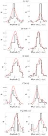 |
Fig. 1. Distribution of the amplitudes (left) and rates (right) of EVPA rotations for each blazar of our sample. The black line shows the histograms, and the red line shows the histograms smoothed with Gaussian kernels. Positive values of the amplitudes and rates correspond to CCW rotations, and negative values correspond to CW rotations. |
Properties of the observed rotations.
Average values of PD (see Cols. 9 and 11 of Table 2) were calculated for three periods: during CCW rotations, during CW rotations, and out of rotations. We followed the assumption that the measured PD follows a beta distribution (Blinov et al. 2016b; Hovatta et al. 2016) with
where p is the PD, and α and β are the parameters of the beta distribution. Hovatta et al. (2016) noted that this method automatically and properly accounts for biasing, and we therefore did not apply debiasing to our data. Thus, the mean value of PD is given by
Column 10 of the Table 2 contains the mean PD of rotations, which have one or no changes of the rotation sign and an amplitude higher than 90 degree. It was calculated without the beta distribution fit because there are only relatively few such rotations.
We note that each of these sources shows an imbalance between the number of CW and CCW rotations (this can also be seen by the skewness of the histograms in Fig. 1). For OJ 287 and CTA 102, the rotations tentatively tend to occur more often in the CW direction, while in other objects in our sample, CCW rotations appear to dominate. To estimate the probability that this imbalance occurs by chance, we calculated the p and σ values of the null-hypothesis that both directions of the EVPA rotations are equally probable. We provide them in Cols. 4 and 5 of Table 2. For all sources, the p values are between 0.034 and 0.006 and the σ values lie between 2 and 3, which means that a preferred direction of EVPA rotations in these five blazars is slightly indicated. For the remaining sample, this tendency is either absent or has a statistical significance (< 2σ).
We assumed that rotations in the preferred and opposite directions may be caused by different mechanisms, and we therefore compared their average properties (see Cols. 6–9 in Table 2). We found no significant differences between the characteristics (amplitudes, rates, and directions) of the rotations in the preferred and opposite directions, except for the case of CTA 102, for which we observed that rotations in the preferred direction are marginally slower according to the t-test (σ = 2.85).
On average, the objects in our sample exhibit several rotations per year in the observer’s system: 4.56 (OJ 287), 4.28 (S5 0716+71), 3.11 (3C 454.3), 1.76 (CTA 102), and 1.26 (PG 1553+113) events per year. Time in the jet system is related to time in the observer system as follows:
This gives the average rotation frequencies in the jet system as follows: 0.93 (OJ 287), 0.06 (S5 0716+71), 0.09 (3C 454.3), 0.95 (CTA 102), and 0.82 (PG 1553+113) events per year.
5. Discussion and conclusions
In this Letter, we reported the finding of a potential preferred direction of EVPA rotations in five blazars. For OJ 287 and CTA 102, the rotations presumably tend to occur more often in the clockwise direction, while S5 0716+71, 3C 454.3, and PG 1553+113 might show a preference for counterclockwise rotations. These results are only tentatively significant and require more observations to clarify them.
Since a preferred direction of the EVPA rotations along with the counter-rotations may imply the action of different production mechanisms, we investigated the mean rotation properties in both the possible preferred and in the opposite directions, as well as the mean polarization properties of our objects out of the rotations.
For five blazars of our sample, we find no notable differences on average, except for CTA 102, for which rotations in the preferred direction are about two times slower than in the opposite direction.
In contrast to previous works (Blinov et al. 2016b; Otero-Santos et al. 2023; Jermak et al. 2016), we did not find that the mean PD during rotations is lower on average than out of rotations. Figure 1 shows that the majority of rotations have a low amplitude, lower than 90 degrees. They were therefore not taken into account in the literature, where this lower limit on the amplitude was imposed. We note that there is a clear anticorrelation between the rotation amplitude and the mean PD value: High-amplitude rotations tend to have lower mean PD value (see Fig. 2). Therefore, when a lower limit is imposed on the amplitude, the observed mean PD value is biased. When we reject all nonmonotonic rotations (with two or more changes in the rotation sign) with an amplitude lower than 90 degrees, we obtain the lower PD value during rotations on average (see Col. 10 of Table 2). Out of 256 rotations that we detected in the five blazars, 104 occur when the observed mean PD value is higher than 10% (see Fig. 2): 68 rotations for OJ 287, 21 rotations for S5 0716+71, 7 rotations for 3C 454.3, 7 rotations for CTA 102, and one rotation for PG 1553+113. These rotations are most likely associated with events in the jet other than random walks caused by turbulence. In the future, we plan to search for connections between EVPA rotations and optical and γ-ray outbursts or changes in the structure of the parsec-scale jet.
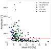 |
Fig. 2. Amplitude vs. mean PD of each observed EVPA rotation. The dashed red line shows the amplitude value of 90°. |
The tentative existence of a preferred direction of EVPA rotations in these five blazars rules out a purely random-walk origin, even for low-amplitude blazars, which are usually considered as insignificant. The existence of rotations in the opposite direction suggests that there are turbulent components in addition to the ordered magnetic field, while the ratio of Ndom to Nobs can reflect the contribution of the ordered component in the total magnetic field geometry associated with the rotation direction of either the black hole or the accretion disk.
Gabuzda (2018) used circular polarization (CP) measurements of 12 AGNs observed at 15 GHz within the MOJAVE3 project (Homan & Lister 2006) to obtain the properties of their magnetic field. The most likely mechanism of CP production is Faraday conversion of linear polarization into CP, while a helical jet magnetic field B geometry can facilitate this process. In the latter case, the sign of the CP is essentially determined by the pitch angle and helicity of the helical field. Thus, there are two independent ways to obtain the magnetic field geometry: via the preferred direction of optical EVPA rotations, and by observing the transverse rotation measure gradient in radio. However, the number of sources considered in Gabuzda (2018) and in our work is too small, and we have only one object in common (CTA 102), so that no statistical inferences can be made. Future works with an increased number of AGNs would enable us to compare these methods directly.
Data availability
Data is available on Zenodo: https://doi.org/10.5281/zenodo.14001086
Imaging X-ray Polarimetry Explorer.
Monitoring Of Jets in Active galactic nuclei with VLBA Experiments.
Acknowledgments
The research is supported by the RSCF grant No 23-22-00121, https://rscf.ru/project/23-22-00121/. This study was based in part on observations conducted using the 1.8 m Perkins Telescope Observatory (PTO) in Arizona, which is owned and operated by Boston University. We thank the anonymous referee for valuable remarks and comments which allowed to improve the paper.
References
- Abdo, A. A., Ackermann, M., Agudo, I., et al. 2010, ApJ, 716, 30 [NASA ADS] [CrossRef] [Google Scholar]
- Blandford, R. D., & Königl, A. 1979, ApJ, 232, 34 [Google Scholar]
- Blandford, R. D., & Rees, M. J. 1978, in BL Lac Objects, ed. A. M. Wolfe, 328 [Google Scholar]
- Blinov, D., & Pavlidou, V. 2019, Galaxies, 7, 46 [NASA ADS] [CrossRef] [Google Scholar]
- Blinov, D., Pavlidou, V., Papadakis, I., et al. 2015, MNRAS, 453, 1669 [NASA ADS] [CrossRef] [Google Scholar]
- Blinov, D., Pavlidou, V., Papadakis, I., et al. 2016a, MNRAS, 462, 1775 [Google Scholar]
- Blinov, D., Pavlidou, V., Papadakis, I. E., et al. 2016b, MNRAS, 457, 2252 [NASA ADS] [CrossRef] [Google Scholar]
- Blinov, D., Pavlidou, V., Papadakis, I., et al. 2018, MNRAS, 474, 1296 [CrossRef] [Google Scholar]
- Britzen, S., Zajaček, M., Gopal-Krishna, et al. 2023, ApJ, 951, 106 [CrossRef] [Google Scholar]
- Cohen, M. H., & Savolainen, T. 2020, A&A, 636, A79 [NASA ADS] [CrossRef] [EDP Sciences] [Google Scholar]
- Cohen, M. H., Aller, H. D., Aller, M. F., et al. 2018, ApJ, 862, 1 [NASA ADS] [CrossRef] [Google Scholar]
- Di Gesu, L., Marshall, H. L., Ehlert, S. R., et al. 2023, Nat. Astron., 7, 1245 [NASA ADS] [CrossRef] [Google Scholar]
- Event Horizon Telescope Collaboration (Akiyama, K., et al.) 2021, ApJ, 910, L13 [Google Scholar]
- Event Horizon Telescope Collaboration (Akiyama, K., et al.) 2024, ApJ, 964, L25 [NASA ADS] [CrossRef] [Google Scholar]
- Gabuzda, D. 2018, Galaxies, 6, 9 [NASA ADS] [CrossRef] [Google Scholar]
- Gabuzda, D. C. 2021, Galaxies, 9, 58 [NASA ADS] [CrossRef] [Google Scholar]
- Gabuzda, D. C., Rastorgueva, E. A., Smith, P. S., & O’Sullivan, S. P. 2006, MNRAS, 369, 1596 [NASA ADS] [CrossRef] [Google Scholar]
- Ghisellini, G., Tavecchio, F., Foschini, L., et al. 2010, MNRAS, 402, 497 [Google Scholar]
- Homan, D. C., & Lister, M. L. 2006, AJ, 131, 1262 [NASA ADS] [CrossRef] [Google Scholar]
- Hovatta, T., Lindfors, E., Blinov, D., et al. 2016, A&A, 596, A78 [NASA ADS] [CrossRef] [EDP Sciences] [Google Scholar]
- Ikejiri, Y., Uemura, M., Sasada, M., et al. 2011, PASJ, 63, 639 [NASA ADS] [Google Scholar]
- Jermak, H., Steele, I. A., Lindfors, E., et al. 2016, MNRAS, 462, 4267 [NASA ADS] [CrossRef] [Google Scholar]
- Jones, T. W. 1988, ApJ, 332, 678 [NASA ADS] [CrossRef] [Google Scholar]
- Jorstad, S. G., Marscher, A. P., Stevens, J. A., et al. 2007, AJ, 134, 799 [NASA ADS] [CrossRef] [Google Scholar]
- Jorstad, S. G., Marscher, A. P., Larionov, V. M., et al. 2010, ApJ, 715, 362 [Google Scholar]
- Kiehlmann, S., Savolainen, T., Jorstad, S. G., et al. 2013, EPJ Web Conf., 61, 06003 [NASA ADS] [CrossRef] [EDP Sciences] [Google Scholar]
- Kikuchi, S., Inoue, M., Mikami, Y., Tabara, H., & Kato, T. 1988, A&A, 190, L8 [NASA ADS] [Google Scholar]
- Larionov, V. M., Jorstad, S. G., Marscher, A. P., et al. 2008, A&A, 492, 389 [NASA ADS] [CrossRef] [EDP Sciences] [Google Scholar]
- Lico, R., Liu, J., Giroletti, M., et al. 2020, A&A, 634, A87 [NASA ADS] [CrossRef] [EDP Sciences] [Google Scholar]
- Lister, M. L., & Smith, P. S. 2000, ApJ, 541, 66 [NASA ADS] [CrossRef] [Google Scholar]
- Marscher, A. P., Jorstad, S. G., D’Arcangelo, F. D., et al. 2008, Nature, 452, 966 [Google Scholar]
- Marscher, A. P., Jorstad, S. G., Larionov, V. M., et al. 2010, ApJ, 710, L126 [Google Scholar]
- Marscher, A. P., Jorstad, S. G., Larionov, V. M., Agudo, I., & Smith, P. S. 2014, Am. Astron. Soc. Meet. Abstr., 224, 221.19 [NASA ADS] [Google Scholar]
- Nalewajko, K. 2010, IJMPD, 19, 701 [NASA ADS] [CrossRef] [Google Scholar]
- Otero-Santos, J., Acosta-Pulido, J. A., Becerra González, J., et al. 2023, MNRAS, 523, 4504 [NASA ADS] [CrossRef] [Google Scholar]
- Raiteri, C. M., Villata, M., D’Ammando, F., et al. 2013, MNRAS, 436, 1530 [Google Scholar]
- Sasada, M., Jorstad, S., Marscher, A. P., et al. 2018, ApJ, 864, 67 [NASA ADS] [CrossRef] [Google Scholar]
- Savchenko, S. S., Morozova, D. A., Jorstad, S. G., et al. 2024, Astrophys. Bull., 79, 186 [NASA ADS] [CrossRef] [Google Scholar]
- Scargle, J. D., Norris, J. P., Jackson, B., & Chiang, J. 2013, ApJ, 764, 167 [Google Scholar]
- Smith, P. S., Montiel, E., Rightley, S., et al. 2009, arXiv e-prints [arXiv:0912.3621] [Google Scholar]
- Urry, C. M., & Padovani, P. 1995, PASP, 107, 803 [NASA ADS] [CrossRef] [Google Scholar]
- Villforth, C., Nilsson, K., Heidt, J., et al. 2010, MNRAS, 402, 2087 [Google Scholar]
- Vlahakis, N. 2006, ASP Conf. Ser., 350, 169 [NASA ADS] [Google Scholar]
- Weaver, Z. R., Jorstad, S. G., Marscher, A. P., et al. 2022, ApJS, 260, 12 [NASA ADS] [CrossRef] [Google Scholar]
- Zhang, H., Chen, X., & Böttcher, M. 2014, ApJ, 789, 66 [NASA ADS] [CrossRef] [Google Scholar]
All Tables
All Figures
|
Fig. 1. Distribution of the amplitudes (left) and rates (right) of EVPA rotations for each blazar of our sample. The black line shows the histograms, and the red line shows the histograms smoothed with Gaussian kernels. Positive values of the amplitudes and rates correspond to CCW rotations, and negative values correspond to CW rotations. |
| In the text | |
|
Fig. 2. Amplitude vs. mean PD of each observed EVPA rotation. The dashed red line shows the amplitude value of 90°. |
| In the text | |
Current usage metrics show cumulative count of Article Views (full-text article views including HTML views, PDF and ePub downloads, according to the available data) and Abstracts Views on Vision4Press platform.
Data correspond to usage on the plateform after 2015. The current usage metrics is available 48-96 hours after online publication and is updated daily on week days.
Initial download of the metrics may take a while.