© The Authors 2024

1. Introduction

The last decades have seen dramatic progress in numerical methods to solve the multi-level radiative transfer problem outside local thermodynamical equilibrium (LTE), so-called non-LTE methods. Starting with the pioneering work of Auer & Mihalas (1969a,b) with relaxing the assumption of LTE (Holweger 1967) and allowing for non-local effects in space by a two-level modeling simplification with active Lyman and Balmer continua. Followed by the successor, “Pandora stars” (Avrett & Loeser 1992) allowing for non-locality in wavelength, including cross-talk between spectral lines and continua. And up to modern 1D and 3D dynamic simulations that can include the effect of non-locality in time due to the non-equilibrium ionization (e.g. Carlsson & Stein 2002) to understand the formation of spectral lines originating from the different layers in the solar atmosphere.

Nowadays, the “Pandora stars” are overtaken by modern state-of-the-art 3D radiative magneto-hydrodynamic (rMHD) simulations (Gudiksen et al. 2011; Vögler et al. 2005; Rempel 2017; Freytag 2013; Wray et al. 2015; Modestov et al. 2024; Iijima & Yokoyama 2015) representing more realistic and detailed atmospheres. The current practice to understand spectra from the dynamic solar atmosphere is to use 3D rMHD simulations in combination with non-LTE radiative transfer codes (Uitenbroek 2001; Pereira & Uitenbroek 2015; Carlsson 1986; Leenaarts & Carlsson 2009; Štěpán & Trujillo Bueno 2013; Gerber et al. 2023) to forward model spectral lines. Once the synthetic profiles are obtained it is essential to understand the basic formation mechanism to confront models with observations. To infer the formation mechanism of a spectral line, one has to investigate its source function, the ratio of the local emissivity to extinction coefficient. The source function is a key quantity in optically thick line formation that describes the weighted local addition of new photons. In modern non-LTE multi-level radiative calculations this information is encoded in the so-called “multi-level source function” (Jefferies 1968; Canfield 1971; Rutten 2021).

The multi-level source function is obtained in terms of ratios of atomic level populations. These level ratios can be given in a general form as the ratio between direct and indirect transition rates between levels. The computation of indirect transition rates, needed for evaluating the multi-level source function, is seldom discussed in the literature. One of the most comprehensive methods for assessing indirect transition rates and probabilities was introduced by Jefferies (1968). However, the physical interpretation of indirect transition probabilities and their origin is not fully explored yet. In this paper, we present a novel approach using Markov chain theory to calculate and interpret indirect transition rates, probabilities, and the multi-level source function. A similar approach was used before by Kastner (1980), Kastner & Bhatia (1980), Kastner (1982) to obtain level populations to compute intensities from optically thin lines, but not to interpret the optically thick multi-level source function. The Markov chain approach will help to interpret optically thick line formation from modern multi-level non-LTE codes and to better quantify the effects of interlocking, which we illustrate with an application to the Lyman series in the solar atmosphere.

The outline of the paper is as follows. In Sect. 2 we introduce three different methods for calculating the multi-level source function and introduce some basic equations used in non-LTE radiative transfer. Section 3 illustrates the use of the Markov chain multi-level source function description on the spectral lines Ly-α, Ly-β, and Ly-γ. We present our discussion in Sect. 4, followed by our concluding remarks in Sect. 5.

2. Methods

2.1. Radiative transfer

The statistical equilibrium and radiative transfer equation are two fundamental equations in solving the non-LTE radiative problem. The transfer equation describes how radiation is emitted, absorbed, and transported through a medium. In contrast, the equations of statistical equilibrium describe how atomic levels are populated under the influence of a radiation field and collisional rates. Solving these equations simultaneously is the main ingredient in computing synthetic spectra.

The transfer equation can be written as:

$$\begin{array}{c}\hfill \frac{\mathrm{d}{I}_{\nu }}{\mathrm{d}s}=j_{\nu }-{\alpha }_{\nu }{I}_{\nu },\end{array}$$(1)

with s the distance measured along the beam, j_ν the emissivity, α_ν the extinction coefficient, and I_ν the intensity. This equation expresses the local addition or subtraction of photons into or out of the beam. A more compact way to express the transfer equation is obtained by expressing it in terms of the optical depth τ_ν and the source function S_ν ≡ j_ν/α_ν:

$$\begin{array}{c}\hfill \frac{\mathrm{d}{I}_{\nu }}{\mathrm{d}{\tau }_{\nu }}=I_{\nu }-S_{\nu }.\end{array}$$(2)

The source function is a key quantity in optically thick line formation. For a spectral line, and assuming complete redistribution (CRD), it can be expressed as:

$$\begin{array}{c}\hfill S_{{\nu }_0}^l=\frac{2h{\nu }_0^3}{c^2}\frac{1}{\frac{g_u{n}_l}{g_l{n}_u}-1},\end{array}$$(3)

where n_u and n_l are respectively the upper and lower level populations, and g_u and g_l the statistical weights. The ratio between upper and lower populations is the critical quantity that varies along the atmosphere. It is typically obtained by assuming statistical equilibrium (i.e., that the populations are constant in time) and solving the system of equations:

$$\begin{array}{c}\hfill {\displaystyle \sum _{j\ne i}}{n}_j{P}_{\mathit{ji}}-n_i{\displaystyle \sum _{j\ne i}}{P}_{\mathit{ij}}=0,\end{array}$$(4)

where the first and second terms describe the rates out and into a level, respectively. P_ij and P_ji are the total transition rates between energy levels, which include collisional and radiative rates.

The level-ratio solution to the statistical equilibrium equations can be expressed as the ratio between direct and indirect transition rates by:

$$\begin{array}{c}\hfill \frac{n_l}{n_u}=\frac{P_{\mathit{ul}}+{\displaystyle {\sum }_u}}{P_{\mathit{lu}}+{\displaystyle {\sum }_l}},\end{array}$$(5)

where P_ul and P_lu are the rates for direct transitions from upper to lower and lower to upper levels, respectively. Indirect transitions are atomic transitions from the upper/lower to the lower/upper level via intermediate atomic levels and are referred to as interlocking, or multi-level detours (Rutten 2021). These indirect transition rates are contained in the variables ∑_u and ∑_l. ∑_u describes the indirect transition rates from the upper level to the lower level through all “non-recurrent” paths available in the atomic level structure. Sections 2.4 and 2.5 cover the meaning and calculation of all “non-recurrent” paths using a Markov chain. ∑_l describes the indirect rates starting from the lower level. The indirect transition rates include information about the strength of interlocking between an atomic transition and all other transitions in an atom.

Using the level ratio solution of the statistical equilibrium equations given by Eq. (5) we can express the line source function more intuitively. This form is often referred to as the multi-level source function, and it includes the effects of indirect atomic transitions. We can write a general expression for the multi-level line source function by decomposing it into three distinct contributions:

$$\begin{array}{c}\hfill S_{{\nu }_0}^l=\sigma {\overline{J}}_{{\nu }_0}+ϵB_{{\nu }_0}(T_{\mathrm{e}})+\eta B_{{\nu }_0}(T^{\star }),\end{array}$$(6)

with

$$\begin{array}{cc}\hfill {\alpha }_{\nu }^l& ={\alpha }_{\nu }^s+{\alpha }_{\nu }^a+{\alpha }_{\nu }^d,\hfill \end{array}$$(7)

$$\begin{array}{cc}\hfill \sigma & ={\alpha }_{\nu }^s/{\alpha }_{\nu }^l,\hfill \end{array}$$(8)

$$\begin{array}{cc}\hfill ϵ& ={\alpha }_{\nu }^a/{\alpha }_{\nu }^l,\hfill \end{array}$$(9)

$$\begin{array}{cc}\hfill \eta & ={\alpha }_{\nu }^d/{\alpha }_{\nu }^l,\hfill \end{array}$$(10)

where ${\overline{J}}_{{\nu }_0}$ indicates the mean radiation field, B_ν0(T_e) a Planck function described by the electron temperature T_e, and B_ν0(T^⋆) the interlocking source function described by characteristic temperature T^⋆. The total line extinction coefficient ${\alpha }_{\nu }^l$ is divided into the scattering extinction ${\alpha }_{\nu }^s$, thermal extinction ${\alpha }_{\nu }^a$, and interlocking or detour extinction ${\alpha }_{\nu }^d$. Interlocking or detour conversion refers to the same physical mechanism; throughout this paper, we use the term interlocking.

In this form of the multi-level source function, σ describes the probability of photon extinction by scattering, ϵ the probability of photon extinction by collisional destruction, and η the probability of photon extinction by interlocking.

Neglecting the third term on the right side of Eq. (6) reduces the multi-level source function to the well-known form of a two-level atom. These two terms cover direct transitions between the upper and lower levels of a transition. The term $\sigma {\overline{J}}_{{\nu }_0}$ describes the source of photons being added to the beam from scattering. The second term ϵ B_ν0(T_e) describes the source of photons into the beam created by collisions with electrons coming from the thermal pool. An intuitive way to think about these two different terms is given by Rutten (2021) introducing the terminology of local in space, non-local in space, and non-local in wavelength. In this context, the thermal part describes photons created locally in space carrying information about the local plasma conditions fully described by the temperature. The scattering part describes the effect of non-locality in space, where thermally created photons coming from different parts of the atmosphere affect the local state of the ensemble of atoms.

The third term in Eq. (6) describes the effect of a multi-level atom onto the upper and lower levels of a transition, commonly referred to as interlocking. The interlocking term contains radiative and collisional transitions connected to the indirect transitions. Therefore, interlocking can cover all three terminologies mentioned above namely, locality in space, non-locality in space, and non-locality in wavelength described by η and B_ν0(T^⋆). The three different sources of extinction in Eq. (7) and the interlocking source function B_ν0(T^⋆) can be given as:

$$\begin{array}{cc}\hfill {\alpha }_{\nu }^s& =A_{\mathit{ul}},\hfill \end{array}$$(11)

$$\begin{array}{cc}\hfill {\alpha }_{\nu }^a& =C_{\mathit{ul}}(1-\exp [-\frac{h{\nu }_0}{k_{\mathrm{B}}{T}_{\mathrm{e}}}]),\hfill \end{array}$$(12)

$$\begin{array}{cc}\hfill {\alpha }_{\nu }^d& =({\displaystyle \sum _u}-\frac{g_l}{g_u}{\displaystyle \sum _l}),\hfill \end{array}$$(13)

$$\begin{array}{cc}\hfill B_{\nu }(T^{\star })& =\frac{2h{\nu }^3}{c^2}{(\frac{g_u{\displaystyle {\sum }_u}}{g_l{\displaystyle {\sum }_l}}-1)}^{-1},\hfill \end{array}$$(14)

where A_ul, C_ul are respectively the Einstein coefficients for spontaneous deexcitation and collisional deexcitation, and the terms ∑_u and ∑_l are the total transition rates from the upper/lower to the lower/upper level via all intermediate levels t, respectively.

The interlocking extinction ${\alpha }_{\nu }^d$ represents the departure from a two-level atom source function. It illustrates that if the indirect transition rate from the upper to the lower level equals the indirect transition rate from the lower to the upper level the multi-level source function approaches the two-level source function.

Not many formalisms are available in the literature to evaluate the multi-level source function for model atoms with many energy levels. The more comprehensive so far are given by Jefferies (1960) and White (1961). Here, we use a different approach to evaluate the multi-level source function, using Markov chain theory to get further insight into how levels are populated indirectly. In addition, we present two other formalisms in Sections 2.2 and 2.3, to compare with.

2.2. Equivalent two-level atom multi-level source function

The most straightforward way to determine the importance of interlocking in the multi-level source function (Eq. (6)) is to make use of the level populations calculated by solving statistical equilibrium (e.g. as an output from non-LTE radiative transfer codes). Instead of analytically removing the level populations and expressing the level ratio solution only in terms of transition rates, one can use the statistical equilibrium equations directly. We refer to this method as the equivalent-two-level-atom approach (ETLA) method because of its close connection to the ETLA method used in the older generations of non-LTE transfer codes, such as “Pandora” (Avrett & Loeser 1992). The idea is to rewrite the statistical equilibrium equations in a way that direct and indirect terms of a transition are grouped:

$$\begin{array}{cc}\hfill n_l(P_{\mathit{lu}}+a_1)& =n_u{P}_{\mathit{ul}}+a_2,\hfill \end{array}$$(15)

$$\begin{array}{cc}\hfill n_u(P_{\mathit{ul}}+a_3)& =n_l{P}_{\mathit{lu}}+a_4,\hfill \end{array}$$(16)

$$\begin{array}{cc}\hfill a_1& ={\displaystyle \sum _{t\ne l,u}}{P}_{\mathit{lt}},\hfill \end{array}$$(17)

$$\begin{array}{cc}\hfill a_2& ={\displaystyle \sum _{t\ne l,u}}\left(n_t{P}_{\mathit{tl}}\right),\hfill \end{array}$$(18)

$$\begin{array}{cc}\hfill a_3& ={\displaystyle \sum _{t\ne l,u}}{P}_{\mathit{ut}},\hfill \end{array}$$(19)

$$\begin{array}{cc}\hfill a_4& ={\displaystyle \sum _{t\ne l,u}}\left(n_t{P}_{\mathit{tu}}\right),\hfill \end{array}$$(20)

with u and l referring to the upper and lower levels of the transition. P_lu and P_ul are the direct transition rates between upper and lower levels. Equations (17)–(20) describe the indirect terms containing the radiative and collisional rates from all transient levels t (excluding the upper and lower level) into and out of the upper and lower levels. The a_i terms contain the information on how strongly a transition is affected by interlocking.

Eqs. (15) and (16) can be solved in terms of level ratios where the indirect transition rates can be written as:

$$\begin{array}{c}\hfill {\displaystyle \sum _u}=\frac{a_2{a}_3}{a_2+a_4},\end{array}$$(21)

$$\begin{array}{c}\hfill {\displaystyle \sum _l}=\frac{a_1{a}_4}{a_2+a_4},\end{array}$$(22)

which can be used to evaluate the multi-level source function.

2.3. Jefferies multi-level source function

Using the multi-level source function formalism by Jefferies (1960, 1968) the solution of the statistical equilibrium in terms of level ratios can be given as:

$$\begin{array}{c}\hfill \frac{n_l}{n_u}=\frac{P_{\mathit{ul}}+{\displaystyle {\sum }_{t\ne l}}{P}_{\mathit{ut}}{q}_{tl,u}}{P_{\mathit{lu}}+{\displaystyle {\sum }_{t\ne u}}{P}_{\mathit{lt}}{q}_{tu,l}},\end{array}$$(23)

where the index t refers to all transient levels between the upper and lower levels of a transition. The indirect rates ∑_u and ∑_l are given by:

$$\begin{array}{cc}\hfill {\displaystyle \sum _u}& ={\displaystyle \sum _{t\ne l}}{P}_{\mathit{ut}}{q}_{tl,u},\hfill \end{array}$$(24)

$$\begin{array}{cc}\hfill {\displaystyle \sum _l}& ={\displaystyle \sum _{t\ne u}}{P}_{\mathit{lt}}{q}_{tu,l},\hfill \end{array}$$(25)

with the indirect transition rates not explicitly involving the level population and introducing q_tl, u and q_tu, l, the indirect transition probabilities. q_tl, u describes the probability that a transition from the transient level t arrives on the lower level before the upper level, and q_tu, l in the opposite direction. The evaluation of q_tl, u and q_tu, l can be found in Jefferies (1968), and involves solving a set of linear equations, similar to the statistical equilibrium equations, to determine the probabilities. These two terms appear relatively abstract, and in the next section, we use a different approach to get insight into the indirect transition probabilities.

2.4. Markov chain multi-level source function

The motivation behind using Markov chain theory is that once we establish a connection to Jefferies’s indirect transition probabilities or the analytical level ratio solution we can use all of the tools available in Markov chain theory to get insight into how levels are statistically populated given some transition rates between levels.

We start by briefly introducing the basic concepts of a Markovian process or Markov chains. A Markovian process is an independent, finite stochastic process where the probability of going from one level to another level does not depend on the past. By the past, we mean that the probability p_ij(n) going from state i to state j after the n-th step does not depend on how the Markov chain reached state i nor on the step count n. In Markov chain theory, the terminology of states is used. Here, we will refer to states as “levels”, as we are dealing with atomic energy levels. Further, we indicate transition probabilities with a lowercase p and transition rates with an uppercase P.

The statistical equilibrium equations use the transition rates P_ij and P_ji, given per second in and out of levels i and j. In the Markov chain description, we transform the transition rates into transition probabilities by:

$$\begin{array}{c}\hfill p_{\mathit{ij}}=P_{\mathit{ij}}/{\displaystyle \sum _i}{P}_{\mathit{ij}}=P_{\mathit{ij}}/P_i,\end{array}$$(26)

where P_i is the total rate out of level i.

A convenient way to represent a Markov chain process is to arrange the transition probabilities between levels as a matrix. We illustrate the transition probability matrix of a n-level atom and five-level atom in Fig. 1. Each column represents the transition probabilities from level i into all other levels j. The indices i and j refer to the atomic level and “not” the matrix rows and columns indices. If one were to exchange matrix columns, the indices would change.

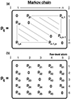Fig. 1. Markov chain transition probability matrix for a n-level (a) and five-level atom (b) with indicated transition probabilities pij.

To analyze a Markov chain process using a probability matrix one has to choose an initial probability vector and multiply it repeatedly with the probability matrix. The probability that the process will be in level n after k steps is given by

$$\begin{array}{c}\hfill {\pi }_k=p^2{\pi }_{k-1}=p{\pi }_{k-2}=p^k{\pi }_0,\end{array}$$(27)

where π₀ is the initial probability vector (its length depends on the model atom size), and p^k contains the probabilities $p_{ij}^n$ that the Markov chain is be found in level j after n-steps, when starting from level i.

We are now interested in a special form of the probability matrix used for absorbing Markov chains. In an absorbing Markov chain, once the absorbing level is reached it is not possible to leave the level again. We can transform the probability matrix shown in Fig. 1a into an absorbing Markov chain by modifying and exchanging columns. The general idea is depicted in Fig. 2a, and involves splitting the probability matrix into four submatrices: I, R, Q, and a zero matrix O. I represents a (n − t)×(n − t) identity matrix that contains the possible transitions after reaching the absorbing level (or levels). The label t refers to the number of transient/intermediate levels. Figure 2b illustrates an absorbing Markov chain probability matrix for a five-level atom. In this example, the absorbing level is the ground level, and therefore the identity matrix has only one element with p₁₁ = 1. The transition probabilities p_1j are set to zero (O matrix), which implies that if the absorbing Markov chain reaches the ground level, it can no longer leave it. R concerns the transition from transient levels to absorbing levels, and has a size of t × (n − t) matrix R. For the five-level atom example, the R matrix is a row vector because it has only one absorbing level. The row vector consists of all transition probabilities into the absorbing level. The last of the four matrices is the t × t matrix Q. It consists of the transition probabilities between the transient levels with zeros in the diagonal.

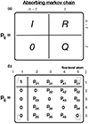Fig. 2. Absorbing Markov chain transition probability matrix for a n-level (a) and five-level atom (b). Panel (a) illustrates the absorbing Markov chain transition probability matrix in canonical form for n-level atom. The submatrices I and 0 represent the identity and zero matrix, respectively related to the absorbing level. Submatrix R contains the transition probabilities from the transient level into the absorbing level. The submatrix Q contains the transition probabilities between transient level. n indicates the number of atomic level whereas t indicates the number of transient level. Panel (b) illustrates an absorbing Markov chain transition probability matrix for a five-level atom with indicated transition probabilities pij.

To simulate a Markov chain process one has to calculate the powers of the transition probability matrix p^k as shown in Eq. (27). We are interested in the case where the power k is sufficiently high so that it is close enough to the limiting matrix $p_{ij}^{\infty }$. This limit case is illustrated in Fig. 3, which can be split into four submatrices: one identity matrix, two zero matrices, and a (I − Q)⁻¹R matrix that contains the probabilities starting from the transient level n_i ending up in the absorbing level n_j. The (I − Q)⁻¹ submatrix contained in $p_{ij}^{\infty }$ is called the fundamental matrix, and is defined as:

$$\begin{array}{c}\hfill \{N_{\mathit{ij}}\}=N={(I-Q)}^{-1},\end{array}$$(28)

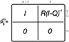Fig. 3. Limiting matrix $p_{ij}^{\infty }$ for a n-level absorbing Markov chain. The submatrices I and 0 represent the identity and zero matrix, respectively. (I − Q)−1 represents the fundamental matrix N. The absorbing probabilities Bij are contained in the submatrix R(I − Q)−1.

where the N_ij are the mean number of times a process is in the transient level n_j before absorption starting from the transient level n_i. Multiplying the fundamental matrix N with the transition probabilities from the transient levels to the absorbing level given by R gives the absorption probabilities B_ij,

$$\begin{array}{c}\hfill \{B_{\mathit{ij}}\}=B=RN,\end{array}$$(29)

where B_ij are the probabilities that an absorbing chain is absorbed in level n_j starting from the transient level n_i. Next, we illustrate how the probabilities B_ij look for a five-level absorbing Markov chain as shown in Fig. 2. For a five-level atom with n = 1 as absorbing level, the absorbing probabilities B₂₁ can be written after grouping terms as:

$$\begin{array}{cc}\hfill B_{21}& =p_{21}+(p_{23}(p_{31}(1-p_{54}{p}_{45})+p_{34}{p}_{41}+p_{34}{p}_{45}{p}_{51}\hfill \\ \hfill & +p_{35}{p}_{51}+p_{35}{p}_{54}{p}_{41})\hfill \\ \hfill & +p_{24}(p_{41}(1-p_{35}{p}_{53})+p_{45}{p}_{51}+p_{45}{p}_{53}{p}_{31}\hfill \\ \hfill & +p_{43}{p}_{31}+p_{43}{p}_{35}{p}_{51})\hfill \\ \hfill & +p_{25}(p_{51}(1-p_{34}{p}_{43})+p_{53}{p}_{31}+p_{53}{p}_{34}{p}_{41}\hfill \\ \hfill & +p_{54}{p}_{41}+p_{54}{p}_{43}{p}_{31}))/det(N)\hfill \\ \hfill & =(R_{21}{N}_{22}+R_{31}{N}_{23}+R_{41}{N}_{24}+R_{51}{N}_{25})/det(N),\hfill \end{array}$$(30)

which illustrates that the total absorption probability B₂₁ is the sum of the direct transition probability plus the probability of all non-recurrent paths from the transient/intermediate levels t to the absorbing state k. A non-recurrent path is defined as a path of the Markov chain that does not pass through the same level twice, excluding the negative terms. The negative terms represent closed loops that correct the different higher-order transition paths to reach the absorbing state. A first-order path is a multiplication of two transition probabilities, a second-order path a multiplication of three transition probabilities, and so forth. The number of negative correction terms depends on the size of the model atom and covers all possible closed loops inside each higher-order transition path.

One can also think of B₂₁ as the product of the sum of the mean occupation times N_t1 and the probability of transitioning to the absorbing level n = 1 divided by the determinant of the fundamental matrix N. The term including R₂₁N₂₂ represents the direct transition probability between the levels n = 2 and n = 1. A general description of the total absorption probability between two levels i and j can be written as:

$$\begin{array}{c}\hfill B_{\mathit{ij}}={\displaystyle \sum _{t\ne j}}{R}_{\mathit{tj}}{N}_{\mathit{it}}/det(N)\end{array}$$(31)

Next, we show that the solution of the statistical equilibrium equation in terms of level ratios can be reproduced by a modified solution of the absorption Markov chain problem. First, we need to choose an appropriate initial probability vector π₀ that will be multiplied by the limiting matrix $p_{ij}^{\infty }$. The correct choice is to use the total rate out of level P_i in the π₀ vector covering the B_ij absorption probabilities. For the case of the B₂₁ probability the choice of the initial probability vector will be π₀ = (0, P₂, 0, 0, 0). This way we transform the transition probabilities p_ik(k indexing overall levels except i) into transition rates P_ik, needed for the solution of the statistical equilibrium equation. The last step is to divide the absorption probabilities B_ij by the fundamental matrix entry N_ii that leads to the cancellation of the determinant of the fundamental matrix N in Eq. (31) and therefore to a different denominator. Applying the steps mentioned above on the five-level case shown in Eq. (30) gives the total rate from level 2 to level 1 connected via all intermediate/transient levels t:

$$\begin{array}{cc}\hfill P_{2t,1}& =P_{21}+(P_{23}(p_{31}(1-p_{54}{p}_{45})+p_{34}{p}_{41}+p_{34}{p}_{45}{p}_{51}\hfill \\ \hfill & +p_{35}{p}_{51}+p_{35}{p}_{54}{p}_{41})\hfill \\ \hfill & +P_{24}(p_{41}(1-p_{35}{p}_{53})+p_{45}{p}_{51}+p_{45}{p}_{53}{p}_{31}\hfill \\ \hfill & +p_{43}{p}_{31}+p_{43}{p}_{35}{p}_{51})\hfill \\ \hfill & +P_{25}(p_{51}(1-p_{34}{p}_{43})+p_{53}{p}_{31}+p_{53}{p}_{34}{p}_{41}\hfill \\ \hfill & +p_{54}{p}_{41}+p_{54}{p}_{43}{p}_{31}))/N_{22}\hfill \\ \hfill & =P_2(R_{21}+(R_{31}{N}_{23}+R_{41}{N}_{24}+R_{51}{N}_{25})/N_{22}).\hfill \end{array}$$(32)

An inconvenient aspect of the above formulation is that one has to analytically group the terms to get to the solution presented in Eq. (30). However, this can be overcome by realizing that the correct grouping of terms is already contained in the limiting matrix $p_{ij}^{\infty }$ for a different absorbing level k. Setting the absorbing level k to one, as presented above, calculates all total transitions ending in the absorbing level starting from the different transient levels. The rows of the fundamental matrix N contain simultaneously the probabilities of starting at the absorbing level k and ending up in each transient level by summing over the rows of the fundamental matrix. Therefore, one can create the correct grouping of terms as in Eq. (30) given by:

$$\begin{array}{c}\hfill P_{ki,j}=P_{\mathit{kj}}+{\displaystyle \sum _{t\ne j,i}}{P}_{\mathit{kt}}{N}_{\mathit{tj}}/N_{\mathit{jj}},\end{array}$$(33)

with the first term describing the direct transition rate and the second term the indirect transition rates. Making use of the total transition rates P_ki, j we can express the solution of the statistical equilibrium equation in terms of level ratios,

$$\begin{array}{c}\hfill \frac{n_l}{n_u}=\frac{P_{ut,l}}{P_{lt,u}}=\frac{P_{\mathit{ul}}+{\displaystyle {\sum }_{t\ne u,l}}{P}_{\mathit{ut}}{N}_{\mathit{tl}}/N_{\mathit{ll}}}{P_{\mathit{lu}}+{\displaystyle {\sum }_{t\ne u,l}}{P}_{\mathit{lt}}{N}_{\mathit{tu}}/N_{\mathit{uu}}},\end{array}$$(34)

with the labels l and u indicating the lower and upper level of a transition. Comparing Eqs. (23)–(34) shows that the Jefferies indirect transition probabilities q_tl, u and q_tu, l represent the terms N_tl/N_ll and N_tu/N_uu in the Markov chain description. These terms portray the ratios between the mean number of times the atom is in level l or u before being absorbed starting from the different levels.

The total indirect rates for the Markov chain description can be written as:

$$\begin{array}{cc}\hfill {\displaystyle \sum _u}& ={\displaystyle \sum _{t\ne u,l}}{P}_{\mathit{ut}}{N}_{\mathit{tl}}/N_{\mathit{ll}}={\displaystyle \sum _{t\ne u,l}}{P}_{\mathit{ut}}{q}_{tl,u},\hfill \end{array}$$(35)

$$\begin{array}{cc}\hfill {\displaystyle \sum _l}& ={\displaystyle \sum _{t\ne u,l}}{P}_{\mathit{lt}}{N}_{\mathit{tu}}/N_{\mathit{uu}}{\displaystyle \sum _{t\ne u,l}}{P}_{\mathit{ut}}{q}_{tu,l}.\hfill \end{array}$$(36)

We can then make use of them to determine the contribution of each intermediate level i to the interlocking source function:

$$\begin{array}{c}\hfill B_{\nu }(T^{\star })={\displaystyle \sum _i}{B}_{\nu }^{{\gamma }_i}(T^{\star }){\gamma }_i,\end{array}$$(37)

where

$$\begin{array}{cc}\hfill {\gamma }_i& =\frac{g_u{P}_{\mathit{ui}}{q}_{il,u}-g_l{P}_{\mathit{li}}{q}_{iu,l}}{g_u{\displaystyle {\sum }_u}-g_l{\displaystyle {\sum }_l}},\hfill \end{array}$$(38)

$$\begin{array}{cc}\hfill B_{\nu }^{{\gamma }_i}(T^{\star })& =\frac{2h{\nu }^3}{c^2}{(\frac{g_u{P}_{\mathit{ui}}{q}_{il,u}}{g_l{P}_{\mathit{li}}{q}_{iu,l}}-1)}^{-1}.\hfill \end{array}$$(39)

Higher-order transition paths connected to individual intermediate levels contribute to the interlocking source function B_ν0(T^⋆) by:

$$\begin{array}{cc}\hfill B_{\nu }(T^{\star })& ={\displaystyle \sum _i}{\gamma }_i{\displaystyle \sum _j}{B}_{\nu }^{{\omega }_j}(T^{\star }){\omega }_j,\hfill \end{array}$$(40)

$$\begin{array}{cc}\hfill {\omega }_j& =\frac{g_u{P}_{\mathit{ui}}{q}_j^{il,u}-g_l{P}_{\mathit{li}}{q}_j^{iu,l}}{g_u{P}_{\mathit{ui}}{q}_{il,u}-g_l{P}_{\mathit{li}}{q}_{iu,l}},\hfill \end{array}$$(41)

$$\begin{array}{cc}\hfill B_{\nu }^{{\omega }_j}(T^{\star })& =\frac{2h{\nu }^3}{c^2}{(\frac{g_u{P}_{\mathit{ui}}{q}_j^{il,u}}{g_l{P}_{\mathit{li}}{q}_j^{iu,l}}-1)}^{-1},\hfill \end{array}$$(42)

where the sum i is the intermediate level and the sum j is the available higher-order transition paths.

The higher-order transition paths are contained in the indirect transition probabilities q_iu, l or q_il, u. As an example, all possible paths for Ly-α in a five-level atom are given by Eqs. (44)–(46). The variables $q_j^{il,u}$ and $q_j^{iu,l}$ represent all possible paths connected to an intermediate level i with the index j summing over the order as in Eqs. (44)–(46).

We show a graphical representation of Eqs. (40)–(42) in Fig. 4. Figure 4 illustrates different higher-order paths for Ly-α contained in the indirect transition probabilities q_31, 2 and q_32, 1 from Eqs. (44) and (47). The red paths highlight the transitions from the lower to the upper level through one or more intermediate levels. The opposite direction (upper to lower level) is shown in blue. These represent a loop that measures the imbalance of transitions between the upper and lower levels through a given path. Summing over all these paths available in the atomic term diagram determines the imbalance of transitions between the upper and lower levels expressed by Eq. (13). If this imbalance is greater than the scattering extinction α_s or thermal extinction α_a, interlocking effects become important and the interlocking source function dominates.

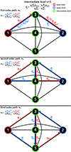Fig. 4. Possible higher-order paths through a five-level atom. Three possible paths are shown for the Ly-α transition through the intermediate level n = 3 expressed by γ3. The green lime color highlights the different intermediate levels. Red arrows indicate the paths from the lower level n = 1 to the upper level n = 2. Blue arrows indicate the paths from the upper to the lower level. Upper panel: first-order paths indicated by ω1 with $q_1^{31,2}=p_{31}(1-p_{54}{p}_{45})$ and $q_1^{32,1}=p_{32}(1-p_{54}{p}_{45})$. Middle panel: second-order paths indicated by ω2 with $q_2^{31,2}=p_{34}{p}_{41}$ and $q_2^{32,1}=p_{34}{p}_{42}$. Bottom panel: third-order paths indicated by ω3 with $q_3^{31,2}=p_{34}{p}_{45}{p}_{51}$ and $q_3^{32,1}=p_{34}{p}_{45}{p}_{52}$.

The interlocking source function B_ν(T^⋆) is defined for a characteristic temperature T^⋆, and can be split into the $B_{\nu }^{{\gamma }_i}(T^{\star })$ components, which represent all paths through intermediate levels. Each $B_{\nu }^{{\gamma }_i}(T^{\star })$ can be further split into $B_{\nu }^{{\omega }_j}(T^{\star })$, which represent the individual paths through intermediate levels. The weighting of the different interlocking source functions to B_ν(T^⋆) is given by γ_i and ω_j. γ_i indicates which intermediate levels are dominant, while ω_j indicates which paths (through the dominant intermediate levels) dominate.

2.5. Application to Lyman series

We want to demonstrate the functionality of the Markov chain multi-level source function description introduced in Sect. 2.4 on the spectral lines Ly-α, Ly-β, and Ly-γ. With the Markov chain description of the multi-level source function, we can express the solution of the statistical equilibrium equation in terms of level ratios with Eq. (34). The level ratio for the Ly-α line can be written with algebraic indirect transition probabilities as:

$$\begin{array}{cc}\hfill \frac{n_1}{n_2}& =\frac{P_{21}+P_{23}·q_{31,2}+P_{24}·q_{41,2}+P_{25}·q_{51,2}}{P_{12}+P_{13}·q_{32,1}+P_{14}·q_{42,1}+P_{15}·q_{52,1}}\hfill \end{array}$$(43)

$$\begin{array}{cc}\hfill q_{31,2}& =(p_{31}(1-p_{54}{p}_{45})+p_{34}{p}_{41}+p_{34}{p}_{45}{p}_{51}+p_{35}{p}_{51}\hfill \\ \hfill & +p_{35}{p}_{54}{p}_{41})/D,\hfill \end{array}$$(44)

$$\begin{array}{cc}\hfill q_{41,2}& =(p_{41}(1-p_{35}{p}_{53})+p_{45}{p}_{51}+p_{45}{p}_{53}{p}_{31}+p_{43}{p}_{31}\hfill \\ \hfill & +p_{43}{p}_{35}{p}_{51})/D,\hfill \end{array}$$(45)

$$\begin{array}{cc}\hfill q_{51,2}& =(p_{51}(1-p_{34}{p}_{43})+p_{53}{p}_{31}+p_{53}{p}_{34}{p}_{41}+p_{54}{p}_{41}\hfill \\ \hfill & +p_{54}{p}_{43}{p}_{31})/D\hfill \end{array}$$(46)

$$\begin{array}{cc}\hfill q_{32,1}& =(p_{32}(1-p_{54}{p}_{45})+p_{34}{p}_{42}+p_{34}{p}_{45}{p}_{52}+p_{35}{p}_{52}\hfill \\ \hfill & +p_{35}{p}_{54}{p}_{42})/D,\hfill \end{array}$$(47)

$$\begin{array}{cc}\hfill q_{42,1}& =(p_{42}(1-p_{35}{p}_{53})+p_{45}{p}_{52}+p_{45}{p}_{53}{p}_{32}+p_{43}{p}_{32}\hfill \\ \hfill & +p_{43}{p}_{35}{p}_{52})/D,\hfill \end{array}$$(48)

$$\begin{array}{cc}\hfill q_{52,1}& =(p_{52}(1-p_{34}{p}_{43})+p_{53}{p}_{32}+p_{53}{p}_{34}{p}_{42}+p_{54}{p}_{42}\hfill \\ \hfill & +p_{54}{p}_{43}{p}_{32})/D\hfill \end{array}$$(49)

$$\begin{array}{cc}\hfill D& =1-p_{34}{p}_{43}-p_{35}{p}_{53}-p_{45}{p}_{54}-p_{34}{p}_{45}{p}_{53}-p_{35}{p}_{54}{p}_{43},\hfill \end{array}$$(50)

for Ly-β as:

$$\begin{array}{cc}\hfill \frac{n_1}{n_3}& =\frac{P_{31}+P_{32}·q_{21,3}+P_{34}·q_{41,3}+P_{35}·q_{51,3}}{P_{13}+P_{12}·q_{23,1}+P_{14}·q_{43,1}+P_{15}·q_{53,1}}\hfill \end{array}$$(51)

$$\begin{array}{cc}\hfill q_{21,3}& =(p_{21}(1-p_{54}{p}_{45})+p_{24}{p}_{41}+p_{24}{p}_{45}{p}_{51}+p_{25}{p}_{51}\hfill \\ \hfill & +p_{25}{p}_{54}{p}_{41})/D,\hfill \end{array}$$(52)

$$\begin{array}{cc}\hfill q_{41,3}& =(p_{41}(1-p_{25}{p}_{52})+p_{42}{p}_{21}+p_{42}{p}_{25}{p}_{51}+p_{45}{p}_{51}\hfill \\ \hfill & +p_{45}{p}_{52}{p}_{21})/D,\hfill \end{array}$$(53)

$$\begin{array}{cc}\hfill q_{51,3}& =(p_{51}(1-p_{24}{p}_{42})+p_{52}{p}_{21}+p_{52}{p}_{24}{p}_{41}+p_{54}{p}_{41}\hfill \\ \hfill & +p_{54}{p}_{42}{p}_{21})/D\hfill \end{array}$$(54)

$$\begin{array}{cc}\hfill q_{23,1}& =(p_{23}(1-p_{54}{p}_{45})+p_{24}{p}_{43}+p_{24}{p}_{45}{p}_{53}+p_{25}{p}_{53}\hfill \\ \hfill & +p_{25}{p}_{54}{p}_{43})/D,\hfill \end{array}$$(55)

$$\begin{array}{cc}\hfill q_{43,1}& =(p_{43}(1-p_{25}{p}_{52})+p_{42}{p}_{23}+p_{42}{p}_{25}{p}_{53}+p_{45}{p}_{53}\hfill \\ \hfill & +p_{45}{p}_{52}{p}_{23})/D,\hfill \end{array}$$(56)

$$\begin{array}{cc}\hfill q_{53,1}& =(p_{53}(1-p_{24}{p}_{42})+p_{52}{p}_{23}+p_{52}{p}_{24}{p}_{43}+p_{54}{p}_{43}\hfill \\ \hfill & +p_{54}{p}_{42}{p}_{23})/D\hfill \end{array}$$(57)

$$\begin{array}{cc}\hfill D& =1-p_{24}{p}_{42}-p_{25}{p}_{25}-p_{45}{p}_{54}-p_{24}{p}_{45}{p}_{52}-p_{25}{p}_{54}{p}_{42},\hfill \end{array}$$(58)

and for Ly-γ as:

$$\begin{array}{cc}\hfill \frac{n_1}{n_4}& =\frac{P_{41}+P_{42}·q_{21,4}+P_{43}·q_{31,4}+P_{45}·q_{51,4}}{P_{14}+P_{12}·q_{24,1}+P_{13}·q_{34,1}+P_{15}·q_{54,1}}\hfill \end{array}$$(59)

$$\begin{array}{cc}\hfill q_{21,4}& =(p_{21}(1-p_{35}{p}_{53})+p_{23}{p}_{31}+p_{23}{p}_{35}{p}_{51}+p_{25}{p}_{51}\hfill \\ \hfill & +p_{25}{p}_{53}{p}_{31})/D,\hfill \end{array}$$(60)

$$\begin{array}{cc}\hfill q_{31,4}& =(p_{31}(1-p_{25}{p}_{52})+p_{32}{p}_{21}+p_{32}{p}_{25}{p}_{51}+p_{35}{p}_{51}\hfill \\ \hfill & +p_{35}{p}_{52}{p}_{21})/D,\hfill \end{array}$$(61)

$$\begin{array}{cc}\hfill q_{51,4}& =(p_{51}(1-p_{23}{p}_{32})+p_{52}{p}_{21}+p_{52}{p}_{23}{p}_{31}+p_{53}{p}_{31}\hfill \\ \hfill & +p_{53}{p}_{32}{p}_{21})/D\hfill \end{array}$$(62)

$$\begin{array}{cc}\hfill q_{24,1}& =(p_{24}(1-p_{35}{p}_{53})+p_{23}{p}_{34}+p_{23}{p}_{35}{p}_{54}+p_{25}{p}_{54}\hfill \\ \hfill & +p_{25}{p}_{53}{p}_{34})/D,\hfill \end{array}$$(63)

$$\begin{array}{cc}\hfill q_{34,1}& =(p_{34}(1-p_{25}{p}_{52})+p_{32}{p}_{24}+p_{32}{p}_{25}{p}_{54}+p_{35}{p}_{54}\hfill \\ \hfill & +p_{35}{p}_{52}{p}_{24})/D,\hfill \end{array}$$(64)

$$\begin{array}{cc}\hfill q_{54,1}& =(p_{54}(1-p_{23}{p}_{32})+p_{52}{p}_{24}+p_{52}{p}_{23}{p}_{34}+p_{53}{p}_{34}\hfill \\ \hfill & +p_{53}{p}_{32}{p}_{24})/D\hfill \end{array}$$(65)

$$\begin{array}{cc}\hfill D& =1-p_{23}{p}_{32}-p_{25}{p}_{52}-p_{35}{p}_{53}-p_{23}{p}_{35}{p}_{52}-p_{25}{p}_{53}{p}_{32}.\hfill \end{array}$$(66)

The above level ratios for Ly-α, Ly-β, and Ly-γ are then used to determine the dominant intermediate level in the interlocking source function given by Eq. (37). Once the dominant intermediate level is known one can determine the dominant loop given by the algebraic expressions for the indirect transition probabilities q_il, u and q_iu, l. The variables D represent all possible closed loops, meaning loops not connected to the upper and lower levels of the atomic transition. With this formalism, we clearly identify which indirect transition(s) create most of the line photons observed in the spectral line of interest.

2.6. Synthetic spectra

We applied our method to spectral lines synthesized from the FALC solar model (Fontenla et al. 1993), a commonly used 1D plane-parallel and static model of the quiet Sun.

We synthesized the hydrogen Lyman series lines using the RH 1.5D code (Pereira & Uitenbroek 2015). RH 1.5D is based on the RH code (Uitenbroek 2001) and solves the multilevel non-LTE radiative transfer problem with overlapping active bound-bound and bound-free transitions in 1D geometry based on the method developed in a series of papers by Rybicki & Hummer (1991, 1992, 1994).

To synthesize the Lyman series lines we used a five-level hydrogen model atom (including the continuum). All hydrogen transitions were treated with the assumption of complete frequency redistribution (CRD) over the line profiles. Further, we included line blends in the Balmer continuum radiation fields in RH 1.5D in the form of a Kurucz line list¹. We only included lines in the Kurucz line list that significantly alter the Balmer continuum radiation field (line list taken from Krikova et al. 2023) affecting the hydrogen ionization in the atmosphere (see e.g. Carlsson & Stein 2002).

From the converged solution of RH 1.5D, we extracted the transition rates for all relevant transitions, and used them to build the population ratios and the multi-level source functions using different methods.

3. Results

First, we quantified how accurate the Markov chain level ratio solution is compared to the ETLA and Jefferies method. In Fig. 5 we compare the three different methods for the ratio n₂/n₁. From Fig. 5a it is clear that the Markov chain solution for the level ratio agrees very well with the solution from RH. The absolute relative error (Fig. 5b) between the three methods and the RH solution stays below 0.1% throughout the atmosphere. The largest errors occur in the transition region. The absolute errors from the Markov chain and Jefferies methods are similar throughout the atmosphere, but the ETLA method shows a deviation close to the temperature minimum. We find a similar behavior for other level population ratios except that the ETLA method shows a lower error in the lower part of the atmosphere (below 0.5 Mm). The accuracy of the indirect transition probabilities are shown in Fig. 5c and Fig. 5d. The Markov chain description’s analytical and numerical indirect transition probabilities match those calculated with the Jefferies method.

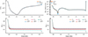Fig. 5. Accuracy of the Markov chain level ratio solution compared to the ETLA and Jefferies method. Panel (a) compares the RH n2/n1 level ratio solution to the Markov chain solution. Panel (b) compares the absolute relative error of the ETLA, Jefferies, and Markov method against the RH solution. Panel (c) shows the indirect transition probabilities numerically calculated with the Jefferies ($q_{i2,1}^{\mathrm{J}}$) and Markov method ($q_{i2,1}^{{\mathrm{M}}_{\mathrm{num}}}$) for the n2/n1 level ratio. Panel (d) shows the analytical indirect transition probabilities from the Markov method ($q_{i2,1}^{{\mathrm{M}}_{\mathrm{ana}}}$) against Jefferies ($q_{i2,1}^{\mathrm{J}}$).

Ly-α multi-level source function. In Fig. 6 we quantified interlocking on the Ly-α line, computed from the FALC model. From Figure 6b one sees that the Ly-α source function is dominated by scattering from the photosphere to the transition region. This shows that the Ly-α source function is well approximated by a two-level source function. This is illustrated by a diagram in the top left corner of Fig. 6c. The Ly-α source function follows the mean radiation field, which in this case is also equal to the interlocking source function (except in the transition region). The interlocking source function shows a strong rise in the transition region due to the sharp temperature increase. The variation of the mean radiation field ${\overline{J}}_{{\nu }_0}$ in the atmosphere is represented in the Ly-α emergent intensity, shown in Fig. 6c with a central reversal. The emergent intensity of the line profile is coming from narrow heights in the FALC atmosphere, mapping ${\overline{J}}_{{\nu }_0}$ into intensity. The central reversal (wavelength position indicated with a black vertical line) is formed in the topmost part of the FALC atmosphere with an outward decreasing source function after an initial peak in the transition region. This behavior of the source function gives rise to the central depression; the two peaks mark the peak of the source function in the transition region. In summary, the Ly-α source function is non-local in space and is affected by different parts of the atmosphere above the temperature minimum. Two-level scattering is the dominant term in the multi-level source function.

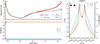Fig. 6. Multi-level source function description of the Ly-α spectral line synthesized from the FALC atmosphere. Panel (a) shows the computed Ly-α source function from RH ($S_{{\nu }_0}^l(T_{\text{exec}})$) as well as the three components describing the multi-level source function, the Planck function Bν0(Te), the mean radiation field $\overline{J}(T_{\mathrm{rad}})$, and the interlocking source function Bν0(T⋆) in units of brightness temperature. The black dashed line (top of the atmosphere) shows the normalized contribution function to intensity for the wavelength position indicated with a black vertical in Panel (c). Panel (b) illustrates the scattering probability σ, destruction probability ϵ, and interlocking probability η. Panel (c) shows the emergent line profile in units of brightness temperature as well as the optical depth unity height with the axis to the right. The icon in the top left corner indicates that two-level processes dominate the Ly-α source function.

Ly-β multi-level source function. In Fig. 7 we show the results for Ly-β. For this line, interlocking dominates below the photosphere, which thermalizes the Ly-β source function to the Planck function. Upwards, from the photosphere through the chromosphere up to the transition region, the Ly-β source function becomes a combination of interlocking and scattering. Interlocking contributes ≈45% to the Ly-β source function with the rest coming from the mean radiation field due to scattering. The mean radiation field matches the interlocking source function throughout the FALC atmosphere except in the transition region, where the interlocking source function shows a stronger sensitivity to the temperature rise, such as for Ly-α. This sensitivity of the source function to temperature is reflected in the Ly-β emission profile shown in Fig. 7c; the line core is formed in the transition region. A significant amount of the line core photons of Ly-β are created by interlocking processes, giving rise to the strong Ly-β emission profile. The dominating interlocking process is shown by the diagram in the top left corner of Fig. 7c, indicating a first-order path through the intermediate level n = 2.

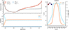Fig. 7. Multi-level source function description of the Ly-β spectral line synthesized from the FALC atmosphere. Figure caption is the same as for Fig. 6 except for the icon. The icon in the top left corner indicates that two-level processes and a first-order interlocking process through the level n = 2 dominates the Ly-β source function.

Figure 8 displays in detail how strongly each intermediate level and path dominates the interlocking source function for Ly-β. From below the photosphere up to the transition region the dominant intermediate level is n = 2, indicated with γ₂ in Fig. 8a. Indirect transitions through the levels n = 4 (γ₄) and n = 5 (γ₅) have a negligible contribution to the interlocking source function. The intermediate level n = 4 has a little contribution only below the surface.

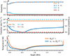Fig. 8. Interlocking source function description of the Ly-β spectral line synthesized from the FALC atmosphere. Panel (a) shows the contribution to interlocking by the different intermediate states, expressed by 38 and paths, expressed by 41. γ2, γ4, and γ5 refers to the intermediate states n = 2, n = 4, and continuum, respectively. ω1 refers to the first-order path connected to p21(1 − p54p45) and p23(1 − p54p45). Panel (b) explains the dominance of the first-order path ω1, with Pij the transition rates and pij transition probabilities between states. Panel (c) shows the contribution of the source function connected to ω1 (blue) to the “total” interlocking source function.

After determining the dominant intermediate level we evaluated which higher-order transition path dominates the indirect transition probabilities q_21, 3 and q_23, 1 highlighted in Eqs. (52) and (55). Fig. 8a highlights that γ₂ is dominated by a first-order interlocking process, ω₁, connected to Ly-α and Hα. This first-order interlocking process is described by a path connecting the upper and lower level of Ly-β with the transition probabilities p₂₁(1 − p₅₄p₄₅) and p₂₃(1 − p₅₄p₄₅). Fig. 8b illustrates the cause of the strong interlocking of Ly-β with Ly-α and Hα by displaying the important terms occurring in ω₁. The transition rate P₃₂ is dominated by the radiative rates given by the spontaneous deexcitation of Hα, and is therefore nearly constant through the atmosphere. The transition rate P₁₂ is dominated by radiative excitation from the ground state by the mean radiation field of Ly-α. Most hydrogen atoms are in the ground state. Therefore the radiative rates R₁₂ are small compared to the spontaneous deexcitation rate of Hα, which leads to orders of magnitude differences between P₃₂ and P₁₂.

The large difference between the transition probabilities p₂₁ and p₂₃ results from the following. Ly-α has the highest spontaneous deexcitation rate of all hydrogen lines in the solar spectrum and is dominating the transitions out of the level n = 2. This is illustrated by p₂₁ being close to one through the FALC atmosphere whereas the probability p₂₃ is relatively small. This specific combination of transition rates and probabilities results in a large imbalance in Eq. (13). This is comparable in size to the scattering extinction (Eq. (11)), making interlocking an important process for Ly-β. Figure 8c shows the contribution of the first-order interlocking source function $B_{\nu }^{{\omega }_1}(T^{\star })$ to the total interlocking source function B_ν(T^⋆).

To summarize, the Ly-β source function is non-local in space and wavelength. The non-locality in wavelength comes from interlocking with Ly-α and Hα. The non-locality in space above the temperature minimum stems from the fact that Ly-α and Hα are strongly scattering.

Ly-γ multi-level source function. Lastly, we turn our attention to Ly-γ, which we show in Fig. 9. Below the photosphere, the source function is dominated by interlocking with the interlocking source function thermalized to the Planck function, similar to Ly-β. From the photosphere up to the transition region interlocking plays a significant role in setting the Ly-γ source function coupled to the temperature, until the temperature minimum. The mean radiation field $\overline{J}(T_{\mathrm{rad}})$ and interlocking source function B_ν0(T^⋆) both approximate well the Ly-γ line source function (except in the transition region). In the transition region, the interlocking source function responds strongly to the temperature rise similar to Ly-α and Ly-β where the Ly-γ line core is formed. Ly-γ is formed from the chromosphere (≈1.35 Mm) up to the transition region (≈2.15 Mm). Its emergent intensity reflects the variation of the interlocking source function between these heights. Next, we want to address which interlocking process sets the behavior of the Ly-γ source function through the FALC atmosphere.

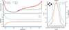Fig. 9. Multi-level source function description of the Ly-γ spectral line synthesized from the FALC atmosphere. Figure caption is the same as for Fig. 6 except for the icon. The icon in the top left corner indicates that two-level processes as well as a first-order interlocking process through the level n = 2 and a first-order and second-order interlocking process through the level n = 3 dominate the Ly-γ source function.

In Fig. 10 we present the contribution to the interlocking source function from the different intermediate levels. Fig. 10a highlights that transitions through two intermediate levels control the interlocking source function. The first intermediate level is n = 2 (γ₂) dominated by a first-order path, while the second intermediate level n = 3 (γ₃) is dominated by a first-order and a second-order path. Below the photosphere, the intermediate level n = 3 dominates the interlocking process through a second-order path described by p₃₂p₂₁ and p₃₂p₂₄ connected to the Hα, Hβ, and Ly-α transitions. Starting from the photosphere, the first-order path through the intermediate level n = 2 becomes increasingly important until approximately the temperature minimum. From that point on, the contribution from intermediate levels n = 2 and n = 3 stay roughly the same level with the intermediate level n = 3 slightly dominating up to the transition region. The contribution to the total interlocking source B_ν(T^⋆) function from the higher-order interlocking source functions $B_{\nu }^{{\omega }_j}(T^{\star })$ from the different intermediate levels can be seen in Fig. 10b.

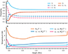Fig. 10. Interlocking source function description of the Ly-γ spectral line synthesized from the FALC atmosphere. Panel (a) shows the contribution to interlocking by the different intermediate states, expressed by Eq. (38) and higher-order paths, expressed by Eq. (41). γ2 and γ3 refers to the intermediate states n = 2 and n = 3. ω1 and ω2 connected to γ3 refer to the first-order path p31(1 − p25p52) and p34(1 − p25p52) and second-order path p32p21 and p32p24, respectively. ω1 connected to γ2 refers to the first-order path connected to p21(1 − p35p53) and p24(1 − p35p53). Panel (b) shows the contributions to the “total” interlocking source function by ω1 through the intermediate state n = 2 as well as ω1 and ω2 through the intermediate state n = 3.

The Ly-γ source function is non-local in space and wavelength, similar to Ly-β. The non-locality in wavelength comes from interlocking with Ly-α, Hα, Hβ, Pa-α affecting the Ly-γ source function. The source function is local in space until the temperature minimum. Further up, the source function becomes non-local in space. The non-locality in space comes from the scattering nature of Ly-α and the other spectral lines affecting Ly-γ.

4. Discussion

The Markov chain description we present in Sect. 2.4 is a different approach to interpreting a multi-level source function with level ratios, which we built by using transition rates from a converged non-LTE solution. It can be used to calculate the indirect transition rates essential to evaluate the multi-level source function and to determine which interlocking processes are important, and where. The indirect transition rates are expressed in terms of indirect transition probabilities as introduced by Jefferies (1960). The absorbing Markov chain approach is a different method of computing the indirect transition probabilities. It can be used numerically and analytically. Our Markov chain approach can be used to get a deeper understanding of the indirect transition probabilities and how the terms build-up for larger model atoms. One realizes that the indirect transition probabilities contain all paths via the intermediate level to the upper/lower without going through the same intermediate level twice (correcting for closed loops). The Markovian description of the multi-level source function can be used to determine which physical processes dominate the source function of a spectral line: scattering, thermal, or interlocking.

We applied the Markovian description of the multi-level source function to the Ly-α, Ly-β, and Ly-γ lines from the FALC model. We find that the Ly-α source function is dominated by two-level scattering due to the large spontaneous photo-deexcitation rate, orders of magnitude larger than the interlocking extinction ${\alpha }_{\nu }^d$ (Eq. (13)), which results in a low photon destruction probability for Ly-α photons (Rutten 2021, 2017a,b). Surprisingly, the Lyman series line source functions above Ly-α start to show a significant contribution from interlocking processes. Ly-β shows a strong coupling with the Ly-α and Hα lines, seemingly in contradiction with the suggestion by Rutten (2017b) that Ly-β is well approximated by two-level atom scattering. Skumanich & Lites (1986) already suggested that Ly-β is strongly coupled with Ly-α and Hα and used a different approach to study the multi-level source function by applying a sensitivity analysis of the statistical equilibrium equations by perturbing the atomic transition rates. Their study also suggested that the Ly-α source function is strongly influenced by the Ly-β and Hα transitions, reflected by the variations of the Ly-α mean radiation field given by the relation

$$\begin{array}{c}\hfill {\overline{J}}_{\mathrm{Ly}-\alpha }\approx \frac{2h{\nu }_0}{c^2}\frac{{\left(B\overline{J}\right)}_{13}}{{\left(B\overline{J}\right)}_{23}}\frac{A_{32}}{A_{31}},\end{array}$$(67)

where A, B, and $\overline{J}$ are the Einstein coefficients for spontaneous deexcitation, radiative excitation, and mean radiation fields, respectively. We find that the direct radiative rates dominate the Ly-α source function following the mean radiation field. However, looking into the Ly-α indirect transition rates we find that a first-order path through the intermediate level n = 3 dominates the indirect transition rates connected to the atomic transitions Hα and Ly-β. Therefore, we find a similar relation for the Ly-α mean radiation field given by:

$$\begin{array}{c}\hfill {\overline{J}}_{\mathrm{Ly}-\alpha }\approx \frac{2h{\nu }_0}{c^2}\frac{{\left(B\overline{J}\right)}_{13}}{{\left(B\overline{J}\right)}_{23}}\frac{p_{32}}{p_{31}},\end{array}$$(68)

which gives the same result as Skumanich & Lites (1986) and is valid up to the transition region of the FALC atmosphere. Our multi-level source function description indicates that the Ly-α radiation field is important for the formation of some hydrogen lines, as suggested by Skumanich & Lites (1986). This is particularly true for hydrogen lines that share an upper or lower level with the Ly-α transition, such as Ly-α, Ly-β, and Hα.

An unexpected coincidence revealed by our approach is that the mean radiation field $\overline{J}(T_{\mathrm{rad}})$ and interlocking source function B_ν0(T^⋆) are equal for Ly-α, Ly-β, and Ly-γ up to the transition region in the FALC atmosphere. This needs a more detailed explanation.

We base our explanation on Eq. (5), which expresses the level ratio solution regarding direct and indirect transition rates between levels. In the multi-level source function description, the ratio of the direct terms n_l/n_u = P_ul/P_lu represents the two-level term $\sigma {\overline{J}}_{{\nu }_0}+ϵB_{{\nu }_0}(T_{\mathrm{e}})$, whereas the ratio of the indirect terms n_l/n_u = ∑_u/∑_l represents the interlocking term η B_ν0(T^⋆). If the direct transition rates dominate, P_ul ≫ ∑_u and P_lu ≫ ∑_u; the multi-level source function is reduced to the two-level approximation (e.g. as with Ly-α). If the indirect transition rates ∑_u and ∑_l become comparable in size to the direct transition rates, interlocking processes become important (as illustrated by Ly-β and Ly-γ). For the mean radiation field ${\overline{J}}_{{\nu }_0}$ to be equal the interlocking source function B_ν0(T^⋆) we need

$$\begin{array}{c}\hfill \frac{n_l}{n_u}\approx \frac{P_{\mathit{ul}}}{P_{\mathit{lu}}}\approx \frac{{\sum }_u}{{\sum }_l}.\end{array}$$(69)

This implies that the spectral line of interest has to be formed under a “two-level” or “interlocking” detailed balance. There are as many upward as downward transitions in direct and indirect transitions between the upper and lower levels of an atomic transition.

To explain the implications of Eq. (69) we draw an analogy to coherent and non-coherent scattering in spectral lines. Coherent scattering assumes no redistribution in the frequency of a line photon after each scattering event; therefore, each frequency position in the spectral line is independent of all other frequency positions in the spectral profile. No cross-talk between photons at different frequencies is allowed. In the case of non-coherent scattering, photons redistribute over the entire line profile (Jefferies 1968). An analogy can be drawn to the effect of interlocking. If a multi-level atom can be approximated by a two-level atom, the line photons arise only from processes related to the upper and lower level of a transition. However, if interlocking becomes important line photons can arise from any transition in the atom, thereby making all transitions a potential photon source for the given spectral line. The mean radiation field of a particular transition becomes a function of the mean radiation field of one or more transitions of an atom, as indicated by Eq. (68). Therefore, if the indirect transition rates become comparable to the direct transition rates, interlocking can have a strong influence on the mean radiation field of a line, leading to a two-level detailed balance.

The effect of a two-level detailed balance can lead to a misinterpretation of the physical mechanism dominating the line source function. One might conclude that the line source function is represented by the two-level approximation very accurately, when in fact the indirect transition rates dominate over the direct transition rates. Therefore, one should always compute the indirect transition rates ∑_u and ∑_l and compare them to the direct transition rates. Ly-β and Ly-γ are great examples where a two-level source function approximation would lead to an incorrect classification of the physical mechanism dominating the line source function.

The multi-level source function we introduce in Sect. 2.4 is valid only under CRD. The more general assumption of PRD over the line profile would result in a multi-level source function that includes the different wavelength-dependent line profiles for emission, absorption, and stimulated emission. The PRD line source function would become wavelength-dependent and more applicable for resonance lines like Ly-α. However, the dominant physical mechanism dominating the line source should not change because the level ratios are wavelength-independent. It would mainly depend on how strongly the assumption of PRD changes the mean radiation fields connected to the different spectral lines influencing the transition probabilities used for the absorption Markov chain. One could include some effects of PRD by assuming that the stimulated emission and absorption profiles are equal ϕ_lu = χ_ul. This makes the source function wavelength dependent and one can write the lines source function given in Eq. (6) as:

$$\begin{array}{c}\hfill S_{\nu }^{\mathrm{PRD}}=S_{{\nu }_0}^{\mathrm{l}}\frac{{\psi }_{\mathit{ul}}}{{\varphi }_{\mathit{lu}}},\end{array}$$(70)

partly including PRD effects.

Many spectral lines formed in the solar chromosphere are classified as (two-level) scattering lines due to their low photon destruction probabilities, such as Ca II H & K, the Ca II infrared triplet, Mg II h & k, the Mg I b triplet, the Na I D doublet lines, as well as the Ly-β line. For these spectral lines, the source functions follow mostly the mean radiation field ${\overline{J}}_{\nu }$, which suggests two-level scattering as a good approximation. However, our results for Ly-β suggest that having $S_{\nu }^l\approx {\overline{J}}_{\nu }$ is a necessary but not sufficient condition to classify a line as (two-level) scattering. Ly-β is strongly influenced by interlocking effects, formed under a “two-level” detailed balance, which implies the need to compare the indirect against the direct transition rates.

To classify chromospheric spectral lines based on the processes that create most of the observed line photons, namely two-level or interlocking one has to calculate the indirect transition rates to evaluate the multi-level source function. It would be of interest to apply our multi-level source function description to classify the most important chromospheric spectral lines to get a better understanding on their formation in the solar chromosphere.

Our results on the formation of Ly-β support the fact that Ly-β is affected by cross-redistribution, also known as Raman scattering (Hubeny & Lites 1995). Ly-β is strongly coupled with Ly-α and Hα and therefore scattering between these lines and redistribution of photons will be very effective (Heinzel & Hubeny 1985). As the three hydrogen lines are strongly coupled this might indicate that Hα is an interlocking line and not a two-level scattering line as suggested by Rutten & Uitenbroek (2012). Rutten & Uitenbroek (2012) did not calculate the indirect transition rates explicitly and their Fig. 12 illustrating that Hα is a two-level scattering line could be misleading if Hα is formed under “two-level” detailed balance with ${\overline{J}}_{\nu }\approx B_{{\nu }_0}(T^{\star })$.

We show that absorbing Markov chains can represent the level-ratio solution of the statistical equilibrium equation made up of direct and indirect transition rates. The indirect transition rates are the sum of the transitions per second from the lower/upper level into the individual intermediate levels times an indirect transition probability. The indirect transition probabilities (as introduced by Jefferies 1960) represent all non-coherent paths from the individual intermediate level to the upper/lower level of the atomic transition. Interlocking becomes important if there is a large imbalance of indirect transitions between the upper and lower levels of a transition represented by a multi-level source function. The multi-level source function can help interpret spectral line formation from modern multi-level non-LTE calculation as illustrated on Ly-α, Ly-β, and Ly-γ. Ly-β and Ly-γ are strongly influenced by interlocking and formed under “two-level” or interlocking detailed balance that gives ${\overline{J}}_{\nu }\approx B_{{\nu }_0}(T^{\star })$.

Formally, our method is valid only for statistical equilibrium between levels, where ionization is included as one or more levels. However, it may be possible to apply our method also in cases of non-equilibrium ionization by keeping the ionization fraction constant and solving statistical equilibrium only for the excited states of the neutral atom, as done by Krikova et al. (2023). This approximation is valid only for model atoms with a single ionized level.

5. Conclusions

We use Markov chain theory to interpret a specific form of the multi-level source function. In non-LTE radiative transfer, the multi-level source function is a key quantity to interpret optically thick line formation, and it depends on the level-ratio solution of the statistical equilibrium equations. We find that absorbing Markov chains are a valid alternative approach to solving the statistical equilibrium equation in terms of level ratios. A crucial advantage of this new method is that it can be used to quantify the effects of interlocking in multi-level atoms.

The effects of interlocking are described by the indirect transition rates, which quantify the transitions per second through intermediate levels that end up in the lower or upper level of an atomic transition. They are the sum of the transitions per second to the intermediate level times an indirect transition probability. The absorbing Markov chain highlights that indirect transition probabilities, as introduced by Jefferies (1960), represent all paths of an atomic transition from the intermediate level leading to the upper or lower level and not entering the same level twice. This insight into the origin of the indirect transition/probabilities rates combined with Eq. (13) gives a straightforward explanation to when interlocking becomes important. Equations (13), (10), and (6) tell us that if the imbalance of transitions connecting the upper and lower levels through all non-coherent paths becomes greater than the scattering or thermal extinctions, the source function (and therefore the source of photons) is strongly coupled to the formation of other spectral lines at different wavelength positions. Therefore, interlocking is always non-local in wavelength.

We present a general form of the multi-level source function (Eq. (6)) that allows one to determine which higher-order transition path dominates the interlocking source function (Eqs. (37)–(42)). Several previous studies relied upon a more qualitative assessment of interlocking (Bruls et al. 1992; Kneer 2010; Leenaarts et al. 2010; Rutten & Uitenbroek 2012) and did not evaluate the indirect transition rates explicitly.

Our analysis of the formation of Ly-β and Ly-γ highlights that a quantitative assessment of the multi-level source function is necessary to determine the physical process dominating the line source function. By calculating the indirect transition rates we find that Ly-β and Ly-γ can be classified as interlocking lines in the solar FALC model. A qualitative analysis of the source function of Ly-β and Ly-γ such as the two-level approximation or the method used by Rutten & Uitenbroek (2012) can lead to a wrong classification of the source function. As a consequence, one might draw the wrong conclusion about the formation of a spectral line. In particular, if the line is formed under the condition of “two-level” or interlocking detailed balance resulting in ${\overline{J}}_{\nu }\approx B_{{\nu }_0}(T^{\star })$. The Hα line, one of the most studied chromospheric spectral lines might be formed under such a condition. Our analysis hints that Hα might be stronglyg interlocked with Ly-α and Ly-β. For a definitive answer about the effect of interlockin on Hα and formation, one should perform a quantitative analysis on the source function of Hα using the multi-level source function introduced in Sect. 2.4. The same is true for most of the strong spectral lines formed in the chromosphere: it may be that interlocking is the dominant mechanism setting the source function, and the methodology outline here is ideally suited for such studies.

Acknowledgments

This work has been supported by the Research Council of Norway through its Centers of Excellence scheme, project number 262622. Computational resources have been provided by Sigma2 – the National Infrastructure for High-Performance Computing and Data Storage in Norway. We acknowledge funding support by the European Research Council under ERC Synergy grant agreement No. 810218 (Whole Sun).

References

All Figures

	Fig. 1. Markov chain transition probability matrix for a n-level (a) and five-level atom (b) with indicated transition probabilities pij.
In the text

Fig. 2. Absorbing Markov chain transition probability matrix for a n-level (a) and five-level atom (b). Panel (a) illustrates the absorbing Markov chain transition probability matrix in canonical form for n-level atom. The submatrices I and 0 represent the identity and zero matrix, respectively related to the absorbing level. Submatrix R contains the transition probabilities from the transient level into the absorbing level. The submatrix Q contains the transition probabilities between transient level. n indicates the number of atomic level whereas t indicates the number of transient level. Panel (b) illustrates an absorbing Markov chain transition probability matrix for a five-level atom with indicated transition probabilities pij.

In the text

	Fig. 3. Limiting matrix $p_{ij}^{\infty }$ for a n-level absorbing Markov chain. The submatrices I and 0 represent the identity and zero matrix, respectively. (I − Q)−1 represents the fundamental matrix N. The absorbing probabilities Bij are contained in the submatrix R(I − Q)−1.
In the text

Fig. 4. Possible higher-order paths through a five-level atom. Three possible paths are shown for the Ly-α transition through the intermediate level n = 3 expressed by γ3. The green lime color highlights the different intermediate levels. Red arrows indicate the paths from the lower level n = 1 to the upper level n = 2. Blue arrows indicate the paths from the upper to the lower level. Upper panel: first-order paths indicated by ω1 with $q_1^{31,2}=p_{31}(1-p_{54}{p}_{45})$ and $q_1^{32,1}=p_{32}(1-p_{54}{p}_{45})$. Middle panel: second-order paths indicated by ω2 with $q_2^{31,2}=p_{34}{p}_{41}$ and $q_2^{32,1}=p_{34}{p}_{42}$. Bottom panel: third-order paths indicated by ω3 with $q_3^{31,2}=p_{34}{p}_{45}{p}_{51}$ and $q_3^{32,1}=p_{34}{p}_{45}{p}_{52}$.

In the text

Fig. 5. Accuracy of the Markov chain level ratio solution compared to the ETLA and Jefferies method. Panel (a) compares the RH n2/n1 level ratio solution to the Markov chain solution. Panel (b) compares the absolute relative error of the ETLA, Jefferies, and Markov method against the RH solution. Panel (c) shows the indirect transition probabilities numerically calculated with the Jefferies ($q_{i2,1}^{\mathrm{J}}$) and Markov method ($q_{i2,1}^{{\mathrm{M}}_{\mathrm{num}}}$) for the n2/n1 level ratio. Panel (d) shows the analytical indirect transition probabilities from the Markov method ($q_{i2,1}^{{\mathrm{M}}_{\mathrm{ana}}}$) against Jefferies ($q_{i2,1}^{\mathrm{J}}$).

In the text

Fig. 6. Multi-level source function description of the Ly-α spectral line synthesized from the FALC atmosphere. Panel (a) shows the computed Ly-α source function from RH ($S_{{\nu }_0}^l(T_{\text{exec}})$) as well as the three components describing the multi-level source function, the Planck function Bν0(Te), the mean radiation field $\overline{J}(T_{\mathrm{rad}})$, and the interlocking source function Bν0(T⋆) in units of brightness temperature. The black dashed line (top of the atmosphere) shows the normalized contribution function to intensity for the wavelength position indicated with a black vertical in Panel (c). Panel (b) illustrates the scattering probability σ, destruction probability ϵ, and interlocking probability η. Panel (c) shows the emergent line profile in units of brightness temperature as well as the optical depth unity height with the axis to the right. The icon in the top left corner indicates that two-level processes dominate the Ly-α source function.

In the text

	Fig. 7. Multi-level source function description of the Ly-β spectral line synthesized from the FALC atmosphere. Figure caption is the same as for Fig. 6 except for the icon. The icon in the top left corner indicates that two-level processes and a first-order interlocking process through the level n = 2 dominates the Ly-β source function.
In the text

Fig. 8. Interlocking source function description of the Ly-β spectral line synthesized from the FALC atmosphere. Panel (a) shows the contribution to interlocking by the different intermediate states, expressed by 38 and paths, expressed by 41. γ2, γ4, and γ5 refers to the intermediate states n = 2, n = 4, and continuum, respectively. ω1 refers to the first-order path connected to p21(1 − p54p45) and p23(1 − p54p45). Panel (b) explains the dominance of the first-order path ω1, with Pij the transition rates and pij transition probabilities between states. Panel (c) shows the contribution of the source function connected to ω1 (blue) to the “total” interlocking source function.

In the text

Fig. 9. Multi-level source function description of the Ly-γ spectral line synthesized from the FALC atmosphere. Figure caption is the same as for Fig. 6 except for the icon. The icon in the top left corner indicates that two-level processes as well as a first-order interlocking process through the level n = 2 and a first-order and second-order interlocking process through the level n = 3 dominate the Ly-γ source function.

In the text

Fig. 10. Interlocking source function description of the Ly-γ spectral line synthesized from the FALC atmosphere. Panel (a) shows the contribution to interlocking by the different intermediate states, expressed by Eq. (38) and higher-order paths, expressed by Eq. (41). γ2 and γ3 refers to the intermediate states n = 2 and n = 3. ω1 and ω2 connected to γ3 refer to the first-order path p31(1 − p25p52) and p34(1 − p25p52) and second-order path p32p21 and p32p24, respectively. ω1 connected to γ2 refers to the first-order path connected to p21(1 − p35p53) and p24(1 − p35p53). Panel (b) shows the contributions to the “total” interlocking source function by ω1 through the intermediate state n = 2 as well as ω1 and ω2 through the intermediate state n = 3.

In the text

References

- Auer, L. H., & Mihalas, D. 1969a, ApJ, 156, 157 [CrossRef] [Google Scholar]
- Auer, L. H., & Mihalas, D. 1969b, ApJ, 156, 681 [NASA ADS] [CrossRef] [Google Scholar]
- Avrett, E. H., & Loeser, R. 1992, ASP Conf. Ser., 26, 489 [NASA ADS] [Google Scholar]
- Bruls, J. H. M. J., Rutten, R. J., & Shchukina, N. G. 1992, A&A, 265, 237 [NASA ADS] [Google Scholar]
- Canfield, R. C. 1971, A&A, 10, 54 [NASA ADS] [Google Scholar]
- Carlsson, M. 1986, Uppsala Astron. Obs. Rep., 33, 2 [Google Scholar]
- Carlsson, M., & Stein, R. F. 2002, ApJ, 572, 626 [Google Scholar]
- Fontenla, J. M., Avrett, E. H., & Loeser, R. 1993, ApJ, 406, 319 [Google Scholar]
- Freytag, B. 2013, Mem. Soc. Astron. Ital. Suppl., 24, 26 [Google Scholar]
- Gerber, J. M., Magg, E., Plez, B., et al. 2023, A&A, 669, A43 [NASA ADS] [CrossRef] [EDP Sciences] [Google Scholar]
- Gudiksen, B. V., Carlsson, M., Hansteen, V. H., et al. 2011, A&A, 531, A154 [NASA ADS] [CrossRef] [EDP Sciences] [Google Scholar]
- Heinzel, P., & Hubeny, I. 1985, NATO ASI Seri. C, 152, 137 [NASA ADS] [Google Scholar]
- Holweger, H. 1967, Z. Astrophys., 65, 365 [NASA ADS] [Google Scholar]
- Hubeny, I., & Lites, B. W. 1995, ApJ, 455, 376 [NASA ADS] [CrossRef] [Google Scholar]
- Iijima, H., & Yokoyama, T. 2015, ApJ, 812, L30 [NASA ADS] [CrossRef] [Google Scholar]
- Jefferies, J. T. 1960, ApJ, 132, 775 [NASA ADS] [CrossRef] [Google Scholar]
- Jefferies, J. T. 1968, Spectral line formation (Waltham, Mass: Blaisdell) [Google Scholar]
- Kastner, S. O. 1980, Ap&SS, 68, 245 [NASA ADS] [CrossRef] [Google Scholar]
- Kastner, S. O. 1982, A&A, 108, 361 [NASA ADS] [Google Scholar]
- Kastner, S. O., & Bhatia, A. K. 1980, Phys. Rev. A, 22, 560 [NASA ADS] [CrossRef] [Google Scholar]
- Kneer, F. 2010, Mem. Soc. Astron. It., 81, 604 [NASA ADS] [Google Scholar]
- Krikova, K., Pereira, T. M. D., & Rouppe van der Voort, L. H. M. 2023, A&A, 677, A52 [NASA ADS] [CrossRef] [EDP Sciences] [Google Scholar]
- Leenaarts, J., & Carlsson, M. 2009, ASP Conf. Ser., 415, 87 [Google Scholar]
- Leenaarts, J., Rutten, R. J., Reardon, K., Carlsson, M., & Hansteen, V. 2010, ApJ, 709, 1362 [NASA ADS] [CrossRef] [Google Scholar]
- Modestov, M., Khomenko, E., Vitas, N., et al. 2024, Sol. Phys., 299, 23 [NASA ADS] [CrossRef] [Google Scholar]
- Pereira, T. M. D., & Uitenbroek, H. 2015, A&A, 574, A3 [NASA ADS] [CrossRef] [EDP Sciences] [Google Scholar]
- Rempel, M. 2017, ApJ, 834, 10 [Google Scholar]
- Rutten, R. J. 2017a, IAU Symp., 327, 1 [NASA ADS] [Google Scholar]
- Rutten, R. J. 2017b, A&A, 598, A89 [NASA ADS] [CrossRef] [EDP Sciences] [Google Scholar]
- Rutten, R. J. 2021, ArXiv e-prints [arXiv:2103.02369] [Google Scholar]
- Rutten, R. J., & Uitenbroek, H. 2012, A&A, 540, A86 [NASA ADS] [CrossRef] [EDP Sciences] [Google Scholar]
- Rybicki, G. B., & Hummer, D. G. 1991, A&A, 245, 171 [NASA ADS] [Google Scholar]
- Rybicki, G. B., & Hummer, D. G. 1992, A&A, 262, 209 [NASA ADS] [Google Scholar]
- Rybicki, G. B., & Hummer, D. G. 1994, A&A, 290, 553 [NASA ADS] [Google Scholar]
- Skumanich, A., & Lites, B. W. 1986, ApJ, 310, 419 [NASA ADS] [CrossRef] [Google Scholar]
- Štěpán, J., & Trujillo Bueno, J. 2013, A&A, 557, A143 [NASA ADS] [CrossRef] [EDP Sciences] [Google Scholar]
- Uitenbroek, H. 2001, ApJ, 557, 389 [Google Scholar]
- Vögler, A., Shelyag, S., Schüssler, M., et al. 2005, A&A, 429, 335 [Google Scholar]
- White, O. R. 1961, ApJ, 134, 85 [NASA ADS] [CrossRef] [Google Scholar]
- Wray, A. A., Bensassi, K., Kitiashvili, I. N., Mansour, N. N., & Kosovichev, A. G. 2015, ArXiv e-prints [arXiv:1507.07999] [Google Scholar]