| Issue |
A&A
Volume 689, September 2024
|
|
|---|---|---|
| Article Number | A217 | |
| Number of page(s) | 11 | |
| Section | Extragalactic astronomy | |
| DOI | https://doi.org/10.1051/0004-6361/202450319 | |
| Published online | 13 September 2024 | |
The restless population of bright X-ray sources of NGC 3621
1
Center for Astrophysics | Harvard & Smithsonian, 60 Garden Street, Cambridge, MA, 02138
USA
2
Dipartimento di Fisica, Università degli Studi di Roma “Tor Vergata”, via della Ricerca Scientifica 1, I-00133
Roma, Italy
3
INAF – Osservatorio Astronomico di Roma, Via Frascati 33, I-00078
Monteporzio Catone, Italy
4
INAF – Osservatorio Astronomico di Brera, Via E. Bianchi 46, I-23807
Merate (LC), Italy
5
Department of Physics, Astrophysics, University of Oxford, Denys Wilkinson Building, Keble Road, OX1 3RH
Oxford, UK
6
Scuola Universitaria Superiore IUSS Pavia, Palazzo del Broletto, piazza della Vittoria 15, I-27100
Pavia, Italy
7
INAF – Istituto di Astrofisica Spaziale e Fisica Cosmica di Milano, Via A. Corti 12, I-20133
Milano, Italy
8
Department of Electronics, Information and Bioengineering, Politecnico di Milano, Via G. Ponzio, 34, I-20133
Milan, Italy
9
INAF – IASF Palermo, Via Ugo La Malfa, 153, I-90146
Palermo, Italy
Received:
10
April
2024
Accepted:
27
June
2024
We report on the multi-year evolution of the population of X-ray sources in the nuclear region of NGC 3621 based on Chandra, XMM-Newton, and Swift observations. Among these, two sources, X1 and X5, after their first detection in 2008, seem to have faded below the detectability threshold, a most interesting fact as X1 is associated with the active galactic nucleus (AGN) of the galaxy. Two other sources, X3 and X6, are presented for the first time, the former showing a peculiar short-term variability in the latest available dataset, suggesting an egress from eclipse, and hence belonging to the handful of known eclipsing ultra-luminous X-ray sources. One source, X4, previously known for its heartbeat (i.e. a characteristic modulation in its signal with a period of ≈1 h), shows a steady behaviour in the latest observation. Finally, the brightest X-ray source in NGC 3621, here labelled X2, shows steady levels of flux across all the available datasets, but a change in its spectral shape, reminiscent of the behaviours of Galactic disc-fed X-ray binaries.
Key words: accretion / accretion disks / galaxies: active / galaxies: individual: NGC 3621 / galaxies: nuclei / X-rays: binaries / X-rays: general
© The Authors 2024
 Open Access article, published by EDP Sciences, under the terms of the Creative Commons Attribution License (https://creativecommons.org/licenses/by/4.0), which permits unrestricted use, distribution, and reproduction in any medium, provided the original work is properly cited.
This article is published in open access under the Subscribe to Open model. Subscribe to A&A to support open access publication.
1. Introduction
Ultraluminous X-ray sources (ULXs) are defined as off-nuclear sources with an isotropic luminosity exceeding the 1039 erg/s threshold (see Kaaret et al. 2017; Fabrika et al. 2021; King et al. 2023 and references therein for recent reviews). The idea behind this definition is to include all sources with a luminosity exceeding the Eddington limit for a black hole (BH) of ≈10 M⊙ and to exclude sources powered by accretion onto a supermassive black hole (SMBH), which usually reside in the nuclei of their host galaxies, and are hence dubbed active galactic nuclei (AGN).
Ultraluminous X-ray sources are interpreted as binary systems powered by accretion onto a compact object and, given their extreme luminosities, offer the opportunity to study either accretion at or above the Eddington limit for neutron stars (NSs) and stellar mass BHs, or unusually massive BHs, with masses in the range 102–105 M⊙, known as intermediate-mass black holes (IMBHs). The most extreme example of super-Eddington accretion is probably NGC 5907 ULX, a ULX pulsar containing an accreting NS, whose luminosity exceeds its Eddington limit by almost three orders of magnitude (Israel et al. 2016).
On the other hand, ESO 243-49 HLX-1, with a peak luminosity as high as 1042 erg/s is, to date, considered the most convincing candidate IMBH (Farrell et al. 2009). This source was discovered owing to its luminosity and to its great distance from its host galaxy centre. However, a large fraction of IMBHs are expected to be hosted in the nuclear regions of their host galaxies (Chilingarian et al. 2018), and even wandering IMBHs are predicted to undergo periods of high luminosity when transiting through galactic nuclei (Weller et al. 2023).
The spectra of ULXs are generally characterised by two thermal components, usually described with black bodies or modified accretion disc black bodies, that dominate the emission above and below ∼1 keV. A third, high-energy component, usually modelled with a cutoff power law (e.g. Walton et al. 2018), is also observed in all the ULX pulsars, suggesting that it descends from an accretion column above the NS. In a super-Eddington accretion scenario, the lower-energy thermal component is associated with either the emission from an optically thick outflow (e.g. Poutanen & Beloborodov 2006) or an outer disc (observed temperatures of ∼0.2 − 0.5 keV), while the higher-energy component could be an inner disc emission deprived of winds (temperatures of ∼1 − 2 keV).
NGC 3621 is a field spiral galaxy in the Hydra constellation, at a distance of 6.7 Mpc (Tully et al. 2013). Although it is morphologically classified as bulgeless, the nuclear region of NGC 3621, roughly defined as the region within a 2 kpc radius of the galactic centre (corresponding to a projected distance of 1′), is a most interesting environment. By analysing the optical spectrum and stellar dynamic, Barth et al. (2009) assigned a Seyfert 2 classification to the galaxy and inferred an upper limit on the central BH mass of 3 × 10⁶ M⊙. The presence of an AGN in the nucleus of NGC 3621, powered by a particularly light SMBH, was also inferred by the inspection of its infrared emission (Satyapal et al. 2007) and association with an X-ray source (Gliozzi et al. 2009). The lower limit on the BH mass, inferred from the X-ray luminosity of the source associated with the infrared emission lower limit, is about 4 × 10³ M⊙, making it possible that the black hole powering the AGN in NGC 3621 is an IMBH.
In the X-ray band, NGC 3621 has been imaged repeatedly. In 2008 the Chandra visit (ObsID: 9278, PI: Gliozzi, hereafter CXO1) that revealed the X-ray counterpart of the AGN (hereafter X1) also detected two off-nuclear ULXs, with luminosities of about 1039 erg/s, far from the galaxy’s nucleus by about 20″. Gliozzi et al. (2009) labelled these two sources B and C, while in this paper they are referred to as X2 and X5, respectively.
A follow-up observation of NGC 3621, obtained with XMM-Newton in 2017 (ObsID: 0795660101, PI: Annuar, hereafter XMM1), revealed an additional most-interesting source, 4XMM J111816.0–324910, referred to as X4 in this paper. This source was too faint to be noticed in the Chandra observation, while in the XMM-Newton observation its luminosity exceeded the 1039 erg/s threshold, hence earning a classification of transient ULX. Furthermore, in the XMM-Newton observation, this source exhibited a peculiar quasi-periodic modulation in its signal, with a period of ≈1 h. The X-ray spectral and timing analysis, as well as the search for the optical counterpart of this source, are presented in Motta et al. (2020).
The discovery of this last transient ULX prompted extensive Swift/XRT monitoring of NGC 3621, which culminated in a second XMM-Newton observation (ObsID: 0884030101, PI: Motta, hereafter XMM2), obtained in May 2023. Along with X4, two other ULXs (X3 and X6), previously neglected, stand out in both XMM-Newton observations, raising the number of X-ray sources surrounding the nuclear region of NGC 3621 to five. This paper is dedicated to the description of the X-ray behaviour of the ULXs residing in the nuclear region of NGC 3621 as well as its central AGN. Figure 1 shows NGC 3621 in the near-ultraviolet (NUV) band with three insets to highlight the evolution of the ULX population surrounding its nuclear region. The position and nomenclature of the sources analysed in this work are summarised in Table 1.
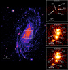 |
Fig. 1. NGC 3621 from a NAO-IRAF image in the NUV band. The inset shows the location of the ULXs described in the paper, in the three epochs of the Chandra and XMM-Newton visits. |
Nomenclature and position for the sources analysed in this work.
The paper is organised as follows. In Sect. 2 we describe the dataset upon which the presented analysis is based and the observational properties of each ULX. In Sect. 3 we discuss the possible nature of each source. Finally, in Sect. 4 we summarise our results.
2. Observational properties
2.1. X-ray dataset
The results presented in this work rely on all the available X-ray observations of NGC 3621 obtained with Chandra, XMM-Newton, and the Neil Gehrels Swift Observatory, and already partially analysed and described by Gliozzi et al. (2009) and Motta et al. (2020). In addition to these data, the bulk of the analysis is based on the observations of NGC 3621 performed with Swift and XMM-Newton in the context of a monitoring campaign of X4.
The Swift–XRT data were retrieved from the science archive1 and reprocessed using the ftool routine xrtpipeline. The count rates and upper limit for each observation (without separating the individual orbits) were computed with the ximage tool sosta and converted into fluxes adopting the best-fitting model of the closest available XMM-Newton or Chandra observation.
XMM-Newton data were downloaded from the science archive2 and reprocessed following the standard procedure with sas v21.0.0 (Gabriel et al. 2004). The light curve of the full observation was inspected and periods of high particle background were excluded from our analysis. For XMM1 we filtered out time intervals during which the background rate was higher than 0.6 and 0.35 cts/s for PN and MOS, respectively. For observation XMM2, we excluded two high background periods at the beginning and at the end of the observation. The data from the EPIC-MOS cameras were merged using the sas tool merge, once verified that the two cameras provided compatible results. To build spectra and light curves, to minimise contamination from nearby sources, counts were extracted from 15″ radius circular regions centred on each source position. Background counts were extracted from nearby 30″ radius circular regions, from source-free portions of the same detector chip of each source. Upper limits were obtained using the sas tool eupper. Spectra, spectral redistribution matrices, and ancillary response files were generated using the dedicated sas tools.
CXO1, taken in sub-array mode, was reprocessed and reduced with the Chandra Interactive Analysis of Observations software package (CIAO, v.4.12; Fruscione et al. 2006) and the CALDB 4.9.0 release of the calibration files. Source counts were extracted, using the CIAO tool srcflux, from regions encompassing a point spread function (PSF) fraction of about 95% (corresponding to roughly 3″ radius circles). Backgrounds were estimated from source-free annular regions, centred on the source position, of 7 and 15 arcsec radii. Spectra, spectral redistribution matrices and ancillary response files were generated using the CIAO script specextract. All reported luminosities are computed assuming the NGC 3621 distance of 6.7 Mpc.
2.2. Spectral analysis
Here we report the X-ray spectra and associated spectral analysis of the X-ray bright sources in the nuclear region of NGC 3621. Spectra already published by Gliozzi et al. (2009) and Motta et al. (2020) will not be analysed further; however, a comprehensive analysis of the multi-epoch spectral evolution of the single sources is presented in Sect. 3.
The spectra were then fed into the spectral fitting package XSPEC (Arnaud 1996) version 12.12.1. Only counts in the energy range 0.3 − 10 keV were considered and, given that all analysed spectra have sufficient counts, the spectra were rebinned to have at least 20 counts per energy bin and the χ2-statistic was adopted. All X-ray spectra were corrected for foreground interstellar absorption adopting the model TBABS, with NH fixed to the Galactic value 6.63 × 1020 cm−2 (HI4PI Collaboration 2016). All the reported values of intrinsic absorption are hence to be considered higher than this foreground value. We adopted abundances from Wilms et al. (2000), with the photoelectric absorption cross-sections from Verner et al. (1996). All reported uncertainties correspond to 1σ, all fluxes are intended as observed, while luminosities are reported as unabsorbed. Spectra extracted from CXO1 were analysed in the 0.5 − 7 keV band, but luminosities are all reported in the 0.3 − 10 keV band to allow for direct comparison.
2.2.1. X1
The AGN, which is labelled X1, is marginally detected in CXO1, described at length in Gliozzi et al. (2009), and not detected in either XMM1 or XMM2, so no further spectral analysis is possible for this source.
2.2.2. X2
The X-ray spectrum of X2 from CXO1 is described in Gliozzi et al. (2009), where it is reproduced by an absorbed power law with NH = (3.4 ± 0.6)×1021 cm−2 and Γ = 2.7 ± 0.3.
The X-ray spectrum of X2 can be reproduced by an absorbed power law in XMM1 as well. The best-fitting parameters are NH = (1.1 ± 0.1)×1021 cm−2 and Γ = 1.87 ± 0.03, corresponding to a statistic of χ2/ν = 241.54/188 ≈ 1.27 (where χ2 is the value of the χ2-statistic and ν the number of degrees of freedom).
In XMM2 the X-ray spectrum of X2 cannot be reproduced satisfactorily with a power law (χ2/ν = 1078.34/263 ≈ 4.1) nor by a combination of a power law and other models. Instead, it can be well reproduced by an absorbed multi-colour disc model, DISKBB in Xspec, with χ2/ν = 287.63/263 ≈ 1.09. Although not specifically requested by the data, we performed a further spectral fit by adding a second thermal component, also modelled with a DISKBB, to be in line with the most recent findings on ULX spectral properties. We note that the fit is marginally improved (χ2/ν = 280.71/261 ≈ 1.07).
At this point, we tried to fit the data from CXO1 and XMM1 with the same absorbed two-thermal component model. We obtained acceptable fits for both epochs, with marginally better χ2 with respect to the single power-law model.
The best-fitting parameters for the two-thermal-component model are reported in Table 2 and the spectrum in the different epochs is shown in Fig. 2.
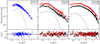 |
Fig. 2. X-ray spectrum (upper panels) and residuals (lower panels) of the source labelled X2 in the three different epochs. Shown in blue are the Chandra data, in black the XMM-Newton/pn data, and in red the merged XMM-Newton/MOS data. The solid lines show the best-fitting models described in the text. The individual components contributing to the model are shown as dotted lines (for XMM1 and XMM2 the two components are shown only for the pn dataset for clarity). |
X-ray spectral properties of the analysed sources.
2.2.3. X3
In CXO1, the source labelled X3 was marginally detected. The low number of counts prevented us from performing the spectral analysis, but by converting the count rate into flux with the best-fitting model described below, we obtained log F = −13.8 ± 0.1 erg/s/cm2, corresponding to a luminosity of log L = 38.3 ± 0.1 erg/s.
In XMM1 and XMM2, the X-ray spectrum of X3 can be well reproduced by an absorbed power law (χ2/ν = 311.67/273 ≈ 1.14). The best-fit parameters of the model are NH = (0.38 ± 0.05)×1021 cm−2 and Γ = 2.18 ± 0.03. The data from the two epochs were fitted simultaneously and the goodness of the fit does not improve freeing either of the two parameters in the two different epochs.
Following the strategy adopted for X2, we tested whether the fit quality could be improved by adopting a two-thermal-component model (DISKBB+DISKBB). We indeed obtained a better statistic (χ2/ν = 273.43/270 ≈ 1.01) that required no intrinsic absorption. The best-fitting parameters are reported in Table 2 and the spectrum in the different epochs is shown in Fig. 3.
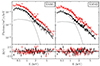 |
Fig. 3. X-ray spectrum (upper panels) and residuals (lower panels) of the source labelled X3 in XMM1 and XMM2 (left and right panels, respectively). Shown in black are the XMM-Newton/pn data and in red the merged XMM-Newton/MOS data. The solid lines show the best-fitting models described in the text; the dotted lines indicate the two thermal components for the sole pn data. |
2.2.4. X4
The X-ray emission of X4 up until late 2017 is fully presented and discussed in a dedicated publication by Motta et al. (2020).
In XMM2, the X-ray spectrum of X4, shown in Fig. 4, can be well reproduced by a two-thermal-component model (DISKBB+DISKBB), with statistic χ2/ν = 94.55/103 ≈ 0.92. The best-fitting parameters of the model are reported in Table 2. To allow for direct comparison with the model adopted for this source in Motta et al. (2020), we also fitted its spectrum with a DISKBB+BBODY model, obtaining a good fit (χ2/ν = 108.48/103 ≈ 1.05) with a black-body temperature for the soft component of 0.26 ± 0.01 keV.
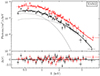 |
Fig. 4. X-ray spectrum (upper panels) and residuals (lower panels) of the source labelled X4 in XMM2. Shown in black are the EPIC/pn and in red the merged EPIC/MOS data. The solid lines show the best-fitting models. The dotted lines indicate the two components for the pn data. |
2.2.5. X5
The X-ray spectrum of X5 as it appeared in CXO1 is described in detail in Gliozzi et al. (2009) and it is reproduced by an absorbed power law with  cm−2 and Γ = 1.6 ± 0.4. Its flux in the 0.3–10 keV band is log F = −12.74 ± 0.04 erg/s/cm2 and its luminosity log L = 39.36 ± 0.04 erg/s.
The source is not detected in either of the two subsequent XMM-Newton observations, and hence no further spectral analysis is possible.
2.2.6. X6
The X6 position fell off the field of view in CXO1, and was in the gap between the two detector chips of the EPIC/pn camera in XMM1, and hence we focus only on the EPIC/MOS data of XMM1 and XMM2 and EPIC/pn data of XMM2.
The data were analysed simultaneously, with all parameters linked together for the normalisation, and the X-ray spectrum of X6 was acceptably reproduced by a simple power-law model, with no additional absorption. We obtained χ2/ν = 102.92/92 ≈ 1.12. The best-fitting slope of the power law is Γ = 1.72 ± 0.03.
In this case too, although the fit was already acceptable with a single power-law model, we fitted a two-thermal-component model to the source, which resulted in a better description of the data (χ2/ν = 91.83/90 ≈ 1.02). The best-fitting parameters are shown in Table 2 and the spectrum in the different epochs is shown in Fig. 5.
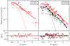 |
Fig. 5. X-ray spectrum (upper panels) and residuals (lower panels) of the source labelled X6 in XMM1 and XMM2 (left and right panels, respectively). Shown in black are the XMM-Newton/pn data and in red the merged XMM-Newton/MOS data. The solid lines show the best-fitting models described in the text, the dotted lines indicate the two thermal components. |
2.3. Long-term light curve
The X-ray light curves of four of the six sources described here are shown in Fig. 6, which reports the luminosity in the 0.3 − 10 keV band as a function of the epoch of observation. The luminosities were obtained by converting the count rates listed in Table B.1 adopting the best-fitting models described above.
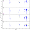 |
Fig. 6. Long-term X-ray light curves of the source X1–X6 (from top to bottom). The magenta, green, and blue points indicate Chandra, XMM-Newton, and Swift/XRT data, respectively. Down-pointing arrows indicate 3σ upper limits. Swift/XRT upper limits are in grey. XMM-Newton/pn and XMM-Newton/MOS upper limits are shown by two different arrows. The count rates on which this figure is built are reported in Table B.1. |
All presented sources show significant variability, often by more than one order of magnitude.
The sources X1 and X5 are not reported, as they fall within the PSF profiles of the much brighter sources X2 and X4, contaminating them in all Swift/XRT observations. Neither X1 nor X5 is detected in either of the two XMM-Newton observations.
2.4. Timing analysis
In this section, we report the timing analysis of the two XMM-Newton observations, focusing on X2, X3, X4, and X6 as X1 and X5 were not detected (see the previous section). We used the SAS tool evselect to extract source events in the 0.3–10 keV band. The light curves and the power density spectra (PDSs) were computed through the XRONOS tasks lcurve and powspec, respectively. The light curves shown in this section were all background subtracted and the bin time was adjusted to ensure there are at least ten counts per bin. Unless otherwise stated, for the analysed sources this requirement corresponds to a bin time of 300 s. A search for coherent periodicity correcting for both a (circular) orbital motion and a first derivative Ṗ of the (possible) spin signal through particle swarm optimisation, an evolutionary algorithm (Pinciroli Vago et al., in prep.) and accelerated search techniques (we followed Rodríguez Castillo et al. 2020) gave negative results. In this section, we report the 3σ upper limits on the pulsed fraction of a signal in the PDSs, computed following Israel & Stella (1996) from the Nyquist frequency νNy down to 1 mHz. The PDSs were computed with the maximum combined time resolution, which in the case of PN+MOS data corresponds to 2.7 s (νNy ≃ 0.18 Hz). For each PDS, we also checked the geometrically rebinned version with a factor of 1.16 and 1.08 (each bin is 16% and 8% larger, respectively, than the previous one) for broad-band features associated with incoherent variability. We found that every PDS was dominated by white noise.
Unless otherwise stated, the errors we report in this section correspond to 1σ (68.3%) confidence ranges. For ease of comparison, we summarise the results of our timing analysis (in particular the upper limits on the pulsed fraction and the rms fractional variation) in Table 3.
Summary of the X-ray pulsed fraction and rms fractional variation upper limits derived by our analysis.
2.4.1. X2
The timing analysis of X2 data from 2017 to 2023 reveals no significant evolution or distinctive features. The top and bottom panels in the left column of Fig. C.1 show the 0.3–10 keV band PDS and the light curve in XMM1, respectively. The top and bottom panels in the right column of Fig. C.1 show the same plots in the same order in XMM2.
2.4.2. X3
Source X3, together with X4, shows the most interesting evolution from a timing point of view. The 0.3–10 keV band PDS and the light curve of XMM1 data are shown, respectively, in the left and right panel of Fig. C.2. No significant feature is detected.
On the other hand, the 0.3–10 keV band light curve from XMM2 (Fig. 7) shows what seems to be the egress of an eclipse. During the first 40 ks of the observation the mean count rate is consistent with a zero flux level. From this we can derive a lower limit on the eclipse duration of approximately 40 ks. The count rate then rapidly rises for approximately 3 ks, only for it to decay back to lower flux rates. After another 1 ks the count rate increases to a steady level of (1.30 ± 0.02)×10−1 cts/s.
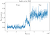 |
Fig. 7. X3 PN+MOS light curve in the 0.3–10 keV band during XMM2. The black dashed line at 51 ks divides the XMM2 light curve into the two regions we considered for our timing analysis. The bin time of the background-subtracted light curve is 300 s. |
In Fig. 8 we report the background-subtracted light curves in the soft (0.3–1 keV) and hard (1–10 keV) band, together with the corresponding hardness ratio (hard/soft). We chose these two bands to have a similar number of photons in both light curves. In this case we adopted a bin time of 1000 s. We do not show the hardness ratio in the first 40 ks of the observations since in this time interval it is dominated by noise due to the low number of collected counts. No clear evolution is visible in the hardness ratio, which can be fitted with a constant. Although a slight rise is visible at ≃40 − 50 ks, its significance is low (< 3σ).
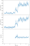 |
Fig. 8. X3 PN+MOS light curve. The top panel show the soft (0.3–1 keV) band, the middle panel the hard (1–10 keV) band, and the bottom panel the hardness ratio of the hard count rate to the soft count rate. We do not show the points in the first 40 ks since the hardness ratio in this range is dominated by noise. The bin time of the background-subtracted light curves is 1000 s. |
Given the low count rate during the first 51 ks of observations (‘Eclipse’ interval) and to avoid artefacts introduced by the eclipse, we computed the PDS (Fig. C.3) only after the first 51 ks (‘High’ interval). We detected no particular feature in the PDS. No coherent signals were detected in either PDS.
2.4.3. X4
The timing analysis of X4, up to and including XMM1, is fully presented and discussed by Motta et al. (2020). In this section, we focus on XMM2.
In XMM1, a striking feature of this source was the presence of a repeating pattern similar to the heartbeat of GRS 1915+105 (Belloni et al. 2000). This feature, however, was absent during the 2023 XMM-Newton observation, as the 0.3–10 keV band PN+MOS light curve shows in Fig. C.4. Figure 9 shows the PDS of 2023 data. For comparison, the dash-dotted line in the PDS shows the frequency of the main peak detected in the PDS in XMM1 data. No significant features can be recognised in the XMM2 PDS.
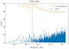 |
Fig. 9. X4 PN+MOS power density spectrum in the 0.3–10 keV band during XMM2. The dash-dotted line at ≃0.3 mHz shows the frequency of the main peak detected in the PDS in XMM1. The yellow dashed line in the original PDS shows the 3.5σ detection threshold. |
2.4.4. X6
For XMM1, we only considered data coming from the two MOS cameras (see the previous section). The 0.3–10 keV band light curve (bin time of 2000 s) and PDS of XMM2 data are shown in the bottom and top panel in the left column of Fig. C.5.
The same plots derived from 2023 data are shown in the two panels in the right column of Fig. C.6. In both observations the source was faint, as can be seen from the light curves, in which time bins consistent with zero count rate can be recognised. The source shows no significant evolution between the two observations.
2.5. Optical counterparts
To attempt an identification of the optical counterpart of the X-ray sources described above, we retrieved the calibrated Hubble Space Telescope (HST) ACS/WFC images of NGC 3621 in three bands: F435W (B), F555W (V), and F814W (I). Unfortunately, no bright source (e.g. a star or background AGN) is present in both the CXO1 and HST dataset to align the images, and no obvious optically bright counterpart is present in the error circles of the X-ray detections, as illustrated in Fig. 10, which shows the RGB HST image with the Chandra error circles superposed for the sources labelled X3 and X5.
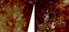 |
Fig. 10. Three-colour composite images of the location of the sources labelled X3 and X5 (on the left and right, respectively) using the HST F814W, F555W, and F435W filters. The white circles show the PSF size (95% uncertainty corresponding to r ≈ 2″) of Chandra. |
3. Discussion
NGC 3621 hosts in its nuclear region a most interesting population of X-ray sources, which, across three long X-ray observations performed with Chandra and XMM-Newton, and several short Swift pointings, revealed a plethora of different behaviours. While four sources have already been studied to some extent and a part of the pertinent X-ray data are publicly available (Gliozzi et al. 2009; Motta et al. 2020), in this work we present a comprehensive description of the ULX population of NGC 3621. We base the bulk of this analysis on proprietary data obtained in the monitoring campaign of one of the presented sources (P.I. Motta).
In this section we discuss, for each source, its possible nature in the light of its X-ray behaviour.
3.1. X1: The AGN
The presence of an AGN in the central region of NGC 3621 was first reported owing to Spitzer detection of emission lines that were incompatible with a burst of star formation (Satyapal et al. 2007). Archival optical images obtained with HST indicate 3 × 10⁶ M⊙ as the upper limit to the mass of the black hole powering the AGN (Barth et al. 2009).
The source labelled here as X1 is marginally detected in the 2009 Chandra observation, and it is spatially coincident with the mid-infrared emission associated with the AGN, and can be most naturally explained as the X-ray counterpart for the AGN, further confirming the presence of an accreting black hole at the centre of NGC 3621. The low X-ray luminosity of the source can be used to place a lower limit on the black hole mass of 4 × 10³ M⊙ (Gliozzi et al. 2009).
However, further investigation of the X-ray properties of this source is prevented by its low luminosity and the presence of the other, much brighter, X-ray sources in its immediate vicinity. The detections of X1 with Swift are unreliable, and the upper limits obtained with both Swift and XMM-Newton are too shallow to place any constraint on the source’s long-term variability. Hence its association with a nuclear X-ray binary cannot be ruled out.
3.2. X2: The brightest source
Source X2 was significantly detected in the three observations we presented. Interestingly, the spectral properties of the source changed over time. While in CXO1 and XMM1 the spectrum is consistent with an absorbed non-thermal emission, the spectrum observed in XMM2 is significantly softer and consistent with black-body-like emission from an accretion disk.
Prompted by the fact that the statistical quality of the fit in XMM2 is marginally improved by adding a second thermal component, we tried fitting the same two-thermal-component models to the previous epochs, obtaining satisfactory fits. While the temperatures of the soft and hard components are always in the 0.2 − 0.5 keV and 1 − 3 keV range, typical of ULXs (Stobbart et al. 2006; Sutton et al. 2012; Gúrpide et al. 2021), the luminosity of the soft component drops by an order of magnitude in XMM2 and the hard components become brighter by a factor of ≈2.5.
While ULXs display a variety of spectra from hard (Γ ≈ 1 if modelled with a power law) to soft (Γ ≈ 3) with no evidence of bimodality (see e.g. Feng & Soria 2011), such a change is reminiscent of the accretion states commonly observed in both persistent and transient Galactic X-ray disk-fed binaries, where a BH or NS system may be found in a hard, soft, or intermediate state (see e.g. De Marco et al. 2022). In this scenario, X2 was consistent with being in the hard state in 2008 and 2017, and in the soft state or, more likely, in a transition state in 2023. The canonical high–soft state seems to be rare in ULXs (Soria et al. 2009). If the parallel holds, in Galactic BH binaries the transition typically takes place at ≈30–50% of the Eddington luminosity, suggesting an extremely heavy stellar or intermediate-mass BH. On the other hand, the possibility of reproducing the spectrum with two thermal components suggests that, similarly to other ULXs, X2 can be interpreted as a case of super-Eddington accretion on a stellar mass compact object.
Unfortunately, the lack of features in the PDS of the source (most likely due to a limited signal-to-noise ratio) prevents us from confirming or ruling out either scenario by employing information from the time variability domain.
3.3. X3: A new eclipsing ULX
The detection of the egress of an eclipse in the light curve of X3 allows us to identify this source as one of the few known eclipsing ULXs (see Sect. 2.3 of Fabrika et al. 2021). We can set a lower limit on the eclipse duration of ≈50 ks. Regarding the orbital period of the system, we can assume as a lower limit the duration of the whole observation ≈90 ks. The presence of an eclipse, moreover, sets a lower limit on the inclination angle of the system i ≳ 75° with respect to the line of sight.
It is interesting to compare X3 with the two eclipsing ULXs in M 51: CXOM51 J132940.0+471237 and CXOM51 J132939.5+471244 (ULX–1 and ULX–2, respectively, in Urquhart & Soria 2016). CXOM51 J132943.3+471135 and CXOM51 J132946.1+471042 (S1 and S2, respectively, in Wang et al. 2018), two other sources in M51 included among the ULXs showing eclipses by Fabrika et al. (2021), have X-ray luminosities LX ≲ 1039 erg s−1 (Wang et al. 2018). It is highly questionable whether they are indeed ULXs, and therefore we do not consider them in our discussion. In the case of ULX–1 and ULX–2, Urquhart & Soria (2016) could only set a lower limit of 70 and 48 ks, respectively, for the eclipse duration. The detection of an ingress and egress in two observations separated by 11 days allowed Urquhart & Soria (2016) to constrain the orbital period of ULX–1 to ≈6 d or ≈12 d. Thanks to their constraints on the orbital period, Urquhart & Soria (2016) could infer a mass of the companion star of ULX–1 in the range Mco ∼ 7 − 31 M⊙, typical of a high-mass X-ray binary (HMXB).
ULX–1 shows an evolution in the hardness ratio, with a softer emission during the eclipse. This is expected, since during an eclipse the central compact object (where the hard X-ray emission arises) is obscured by the companion. Unfortunately, in the case of X3, we could not derive a hardness ratio for the first 40 ks of the eclipse, due to the low number of collected source counts. We can expect, however, a similar evolution in the hardness ratio. Future detections of the eclipse in different observations could allow us to derive a stacked hardness ratio during and outside this phase and verify whether X3 is indeed softer during the eclipse. The presence of a dip at the end of the egress of X3 is probably due to inhomogeneous winds arising from the companion. A similar egress pattern is also observed in LMC X–4, a HMXB (Mco ≃ 18 M⊙) hosting a NS, often observed at super-Eddington luminosities (see Jain et al. 2024 and references therein). Given the similarity between these systems and X3, it is reasonable to assume that X3 is a HMXB whose companion mass is in a comparable range.
The paucity of data regarding this source prevents a deeper discussion. The lower limit on the orbital period (≲90 ks) is shorter than any HMXB orbital period. At the same time, the time span between the two XMM-Newton observations prevents us from deriving meaningful constraints. Finally, no optical counterpart is known for this source, and therefore no radial velocity estimates (which could be used to infer the mass function) are available. Deeper observations are needed to further characterise this peculiar ULX.
3.4. X4: The (not-currently) beating ULX
In the data from 2023, X4 was detected exhibiting a luminosity that aligns with the lower extremity of the spectrum observed towards the end of 2017 (Motta et al. 2020), only slightly below 1039 erg/s. In the 2017 data, this luminosity corresponds to emission phases occurring in the intervals between flares. The spectrum obtained in 2023 is also consistent with those obtained during the low-activity phases in 2017 between the flares.
Unlike the observations from 2017, the most recent light curve analysis does not display any flaring activity. The power density spectrum (PDS) lacks any indication of quasi-periodic modulations around the previously identified heartbeat period of approximately 3500 s (T ≈ 3500 s), with a three-sigma (3σ) upper limit for the quasi-periodic oscillation rms amplitude at 0.28.
When comparing X4 to the archetype of heartbeat sources, GRS 1915+105 (Belloni et al. 1997, 2000), the recently observed behaviour is not unexpected. In GRS 1915+105, similar accretion rates or luminosity levels sometimes coincide with heartbeat events, suggesting that the instability at the base of the flaring is not solely triggered by specific accretion rates. Other factors, such as certain disc properties (e.g. opacity or ionisation state), may play a role in triggering the relevant instability. If the flaring observed in X4 in 2017 shares the same nature as the heartbeats in GRS 1915+105, it could represent an erratic phenomenon that might reoccur in the future at the same or at a different luminosity level.
3.5. X5: Peek-a-boo
The source labelled X5 is convincingly detected only in the first Chandra observation, showing an X-ray spectrum that can be well-modelled by a power law with photon index Γ = 1.6 and a luminosity of about 2.3 × 1039 erg/s, placing it amongst the ULXs. For reasons similar to the one discussed for X1, the Swift detections are unreliable and the only significant upper limits are the ones obtained with XMM-Newton which indicates that the source’s flux dropped by a factor > 5.
Based on the source X-ray spectrum and luminosity, Gliozzi et al. (2009) estimated its mass as 2 × 10³ − 4 M⊙, interpreting this source as an accreting IMBH. However, today’s interpretation of ULXs strongly favours a scenario in which these sources are powered by super-Eddington accretion onto neutron stars (see e.g. Kaaret et al. 2017 and Fabrika et al. 2021 for a review on the topic). Indeed, although the bulk of the ULX population shows steady levels of accretion, a subset exhibits strong variations in their flux, as wide as one order of magnitude, which could be a potential tell-tale of ULX pulsars (e.g. Earnshaw et al. 2018; Song et al. 2020). Another viable explanation for the behaviour of this source is an outburst by an otherwise normal transient X-ray binary, peaking in the ULX regime, as observed in a couple of objects in M 31 (Middleton et al. 2012, 2013; Esposito et al. 2013).
3.6. X6: The faintest sister
The source labelled X6 is the faintest of the population of ULXs in the central region of NGC 3621. Its location fell out of the field of view in the first Chandra observation and in between two detector chips in the EPIC-pn on the first XMM-Newton visit. Although its luminosity lies below the 1039 erg/s in both XMM-Newton observations, it passes the threshold in at least one of the Swift/XRT visits.
Over the different epochs of the XMM-Newton observations, the X-ray flux of X6 remains quite stable, varying only by a factor of about 0.7. No significant change is observed in the X-ray spectral shape of the source: the spectrum in the two available epochs can be satisfactorily reproduced by a power law with a common slope of Γ ≈ 1.6 or with a two thermal component model with temperatures compatible with the population of known ULXs.
X6 does not exhibit any clear short-term variability in any of the XMM-Newton observations, but the source is too faint to put significant constraints on the pulsed fraction of the signal.
Finally, as the other ULXs in NGC 3621, X6 has no clear or bright optical counterpart as too many faint sources crowd the circle error of the XMM-Newton detection.
4. Summary
In this paper, we reported the decade-long behaviour of the population of X-ray bright sources hosted in the nuclear region of NGC 3621. We analysed the long- and short-term variability as well as the spectral evolution of six sources, exploiting archival Chandra data, an extensive Swift monitoring campaign as well as recently acquired XMM-Newton data. The main results of our analysis are the discovery of a new eclipsing binary ULX (X3) and that the ‘heartbeat’ ULX (X4) is currently at an intermediate flux level, but it is not showing its characteristic pulsation. One source (X2) exhibits, across different XMM-Newton observations, changes in its spectral shape with no significant variation in its flux levels, a behaviour common in HMXBs and ULXs. Two sources (X1 and X5) are not detected in any XMM-Newton or Swift visit, and the only available data comes from archival Chandra observations. The picture is completed by the source labelled X6, which, although the faintest of the studied populations, still falls in the ULX regime.
The Table is available at https://doi.org/10.5281/zenodo.12582646.
All plots are available at https://doi.org/10.5281/zenodo.12582691.
Acknowledgments
We thank the anonymous referee for their comments which improved the quality of the paper. M.I. is supported by the AASS Ph.D. joint research programme between the University of Rome ‘La Sapienza’ and the University of Rome ‘Tor Vergata’, with the collaboration of the National Institute of Astrophysics (INAF). PE, GLI, and AT acknowledge financial support from the Italian Ministry for University and Research, through the grants 2022Y2T94C (SEAWIND) and from INAF through LG 2023 BLOSSOM. GLI acknowledges financial support from INAF through grant “INAF-Astronomy Fellowships in Italy 2022 – (GOG). This work was partially supported by the ASI–INAF program I/004/11/5.”
References
- Arnaud, K. A. 1996, ASP Conf. Ser., 101, 17 [Google Scholar]
- Barth, A. J., Strigari, L. E., Bentz, M. C., Greene, J. E., & Ho, L. C. 2009, ApJ, 690, 1031 [NASA ADS] [CrossRef] [Google Scholar]
- Belloni, T., Mendez, M., King, A. R., van der Klis, M., & van Paradijs, J. 1997, ApJ, 479, L145 [NASA ADS] [CrossRef] [Google Scholar]
- Belloni, T., Klein-Wolt, M., Méndez, M., van der Klis, M., & van Paradijs, J. 2000, A&A, 355, 271 [Google Scholar]
- Chilingarian, I. V., Katkov, I. Y., Zolotukhin, I. Y., et al. 2018, ApJ, 863, 1 [Google Scholar]
- De Marco, B., Motta, S. E., & Belloni, T. M. 2022, Handbook of X-ray and Gamma-ray Astrophysics, 58 [Google Scholar]
- Earnshaw, H. P., Roberts, T. P., & Sathyaprakash, R. 2018, MNRAS, 476, 4272 [NASA ADS] [CrossRef] [Google Scholar]
- Esposito, P., Motta, S. E., Pintore, F., Zampieri, L., & Tomasella, L. 2013, MNRAS, 428, 2480 [NASA ADS] [CrossRef] [Google Scholar]
- Fabrika, S. N., Atapin, K. E., Vinokurov, A. S., & Sholukhova, O. N. 2021, Astrophys. Bull., 76, 6 [NASA ADS] [CrossRef] [Google Scholar]
- Farrell, S. A., Webb, N. A., Barret, D., Godet, O., & Rodrigues, J. M. 2009, Nature, 460, 73 [Google Scholar]
- Feng, H., & Soria, R. 2011, New Astron. Rev., 55, 166 [CrossRef] [Google Scholar]
- Fruscione, A., McDowell, J. C., Allen, G. E., et al. 2006, SPIE Conf. Ser., 6270, 62701V [Google Scholar]
- Gabriel, C., Denby, M., Fyfe, D. J., et al. 2004, ASP Conf. Ser., 314, 759 [Google Scholar]
- Gliozzi, M., Satyapal, S., Eracleous, M., Titarchuk, L., & Cheung, C. C. 2009, ApJ, 700, 1759 [NASA ADS] [CrossRef] [Google Scholar]
- Gúrpide, A., Godet, O., Koliopanos, F., Webb, N., & Olive, J. F. 2021, A&A, 649, A104 [NASA ADS] [CrossRef] [EDP Sciences] [Google Scholar]
- HI4PI Collaboration (Ben Bekhti, N., et al.) 2016, A&A, 594, A116 [NASA ADS] [CrossRef] [EDP Sciences] [Google Scholar]
- Huppenkothen, D., Bachetti, M., Stevens, A. L., et al. 2019, ApJ, 881, 39 [Google Scholar]
- Israel, G. L., & Stella, L. 1996, ApJ, 468, 369 [Google Scholar]
- Israel, G. L., Esposito, P., Rodríguez Castillo, G. A., & Sidoli, L. 2016, MNRAS, 462, 4371 [Google Scholar]
- Jain, C., Sharma, R., & Paul, B. 2024, MNRAS, 529, 4056 [NASA ADS] [CrossRef] [Google Scholar]
- Kaaret, P., Feng, H., & Roberts, T. P. 2017, ARA&A, 55, 303 [Google Scholar]
- Kennedy, J., & Eberhart, R. 1995, Proceedings of ICNN’95 - International Conference on Neural Networks, ICNN-95 (IEEE) [Google Scholar]
- King, A., Lasota, J.-P., & Middleton, M. 2023, New Astron Rev., 96, 101672 [NASA ADS] [CrossRef] [Google Scholar]
- Middleton, M. J., Sutton, A. D., Roberts, T. P., Jackson, F. E., & Done, C. 2012, MNRAS, 420, 2969 [NASA ADS] [CrossRef] [Google Scholar]
- Middleton, M. J., Miller-Jones, J. C. A., Markoff, S., et al. 2013, Nature, 493, 187 [Google Scholar]
- Motta, S. E., Marelli, M., Pintore, F., et al. 2020, ApJ, 898, 174 [NASA ADS] [CrossRef] [Google Scholar]
- Poutanen, J., & Beloborodov, A. M. 2006, MNRAS, 373, 836 [NASA ADS] [CrossRef] [Google Scholar]
- Rodríguez Castillo, G. A., Israel, G. L., Belfiore, A., et al. 2020, ApJ, 895, 60 [Google Scholar]
- Satyapal, S., Vega, D., Heckman, T., O’Halloran, B., & Dudik, R. 2007, ApJ, 663, L9 [Google Scholar]
- Song, X., Walton, D. J., Lansbury, G. B., et al. 2020, MNRAS, 491, 1260 [Google Scholar]
- Soria, R., Risaliti, G., Elvis, M., et al. 2009, ApJ, 695, 1614 [NASA ADS] [CrossRef] [Google Scholar]
- Stobbart, A.-M., Roberts, T. P., & Wilms, J. 2006, MNRAS, 368, 397 [Google Scholar]
- Sutton, A. D., Roberts, T. P., Walton, D. J., Gladstone, J. C., & Scott, A. E. 2012, MNRAS, 423, 1154 [NASA ADS] [CrossRef] [Google Scholar]
- Tully, R. B., Courtois, H. M., Dolphin, A. E., et al. 2013, AJ, 146, 86 [NASA ADS] [CrossRef] [Google Scholar]
- Urquhart, R., & Soria, R. 2016, ApJ, 831, 56 [Google Scholar]
- Verner, D. A., Ferland, G. J., Korista, K. T., & Yakovlev, D. G. 1996, ApJ, 465, 487 [Google Scholar]
- Walton, D. J., Fürst, F., Harrison, F. A., et al. 2018, MNRAS, 473, 4360 [Google Scholar]
- Wang, S., Soria, R., Urquhart, R., & Liu, J. 2018, MNRAS, 477, 3623 [NASA ADS] [CrossRef] [Google Scholar]
- Weller, E. J., Pacucci, F., Ni, Y., et al. 2023, MNRAS, 520, 3955 [NASA ADS] [CrossRef] [Google Scholar]
- Wilms, J., Allen, A., & McCray, R. 2000, ApJ, 542, 914 [Google Scholar]
Appendix A: Particle swarm optimisation
Particle swarm optimisation (PSO) is a meta-heuristic optimisation evolutionary algorithm, introduced in Kennedy & Eberhart (1995), that can search for the maximum value of a function  whose analytical expression is unknown. In this work, there are n = 4 independent variables, corresponding to 4 orbital parameters (i.e., Torb, Tasc, aX sin i, and Ṗ/P). Let Cs be the light curve corrected according to a set of orbital parameters s and Ps the corresponding power density spectrum (computed using stingrayHuppenkothen et al. 2019). Then, the dependent variable of f is max(Ps) (i.e., the highest power peak in Ps). Unlike grid search, PSO does not require pre-defining a search grid, which would require making assumptions on the grid step sizes.
Multiple searches are performed on each observation with different PSO hyperparameter values for c1 (nostalgia), c2 (envy), and w (inertia). In particular, c1 ∈ {0.5, 1.0, 1.5}, c2 ∈ {0.5, 1.0, 1.5}, and w ∈ {0.5, 0.75, 1}, for a total of 27 combinations per observation. Different searches consider three different scenarios. If c1 > c2, the algorithm privileges the exploration of diverse candidate sets of orbital parameters; if c1 < c2, the algorithm tends to converge towards local maxima more prematurely, and if c1 ≈ c2, the algorithm balances exploration and convergence towards a maximum solution.
Different results obtained in different searches suggest that (1) the highest powers are not statistically significant (< 3σ), and (2) the optimal orbital parameters combination and frequency vary depending on the search (and not on the source) while having similar powers. Combined with the Ṗ analysis, this approach suggests that the signal is either absent or indistinguishable from noise.
Appendix B: X-ray observations
The journal of the X-ray observations is given in Table B.13
Appendix C: Light curves and PDSs of XMM-Newton observations.
In this section4 we report the remaining light curves and PDSs not shown in the main text.
All Tables
Summary of the X-ray pulsed fraction and rms fractional variation upper limits derived by our analysis.
All Figures
|
Fig. 1. NGC 3621 from a NAO-IRAF image in the NUV band. The inset shows the location of the ULXs described in the paper, in the three epochs of the Chandra and XMM-Newton visits. |
| In the text | |
|
Fig. 2. X-ray spectrum (upper panels) and residuals (lower panels) of the source labelled X2 in the three different epochs. Shown in blue are the Chandra data, in black the XMM-Newton/pn data, and in red the merged XMM-Newton/MOS data. The solid lines show the best-fitting models described in the text. The individual components contributing to the model are shown as dotted lines (for XMM1 and XMM2 the two components are shown only for the pn dataset for clarity). |
| In the text | |
|
Fig. 3. X-ray spectrum (upper panels) and residuals (lower panels) of the source labelled X3 in XMM1 and XMM2 (left and right panels, respectively). Shown in black are the XMM-Newton/pn data and in red the merged XMM-Newton/MOS data. The solid lines show the best-fitting models described in the text; the dotted lines indicate the two thermal components for the sole pn data. |
| In the text | |
|
Fig. 4. X-ray spectrum (upper panels) and residuals (lower panels) of the source labelled X4 in XMM2. Shown in black are the EPIC/pn and in red the merged EPIC/MOS data. The solid lines show the best-fitting models. The dotted lines indicate the two components for the pn data. |
| In the text | |
|
Fig. 5. X-ray spectrum (upper panels) and residuals (lower panels) of the source labelled X6 in XMM1 and XMM2 (left and right panels, respectively). Shown in black are the XMM-Newton/pn data and in red the merged XMM-Newton/MOS data. The solid lines show the best-fitting models described in the text, the dotted lines indicate the two thermal components. |
| In the text | |
|
Fig. 6. Long-term X-ray light curves of the source X1–X6 (from top to bottom). The magenta, green, and blue points indicate Chandra, XMM-Newton, and Swift/XRT data, respectively. Down-pointing arrows indicate 3σ upper limits. Swift/XRT upper limits are in grey. XMM-Newton/pn and XMM-Newton/MOS upper limits are shown by two different arrows. The count rates on which this figure is built are reported in Table B.1. |
| In the text | |
|
Fig. 7. X3 PN+MOS light curve in the 0.3–10 keV band during XMM2. The black dashed line at 51 ks divides the XMM2 light curve into the two regions we considered for our timing analysis. The bin time of the background-subtracted light curve is 300 s. |
| In the text | |
|
Fig. 8. X3 PN+MOS light curve. The top panel show the soft (0.3–1 keV) band, the middle panel the hard (1–10 keV) band, and the bottom panel the hardness ratio of the hard count rate to the soft count rate. We do not show the points in the first 40 ks since the hardness ratio in this range is dominated by noise. The bin time of the background-subtracted light curves is 1000 s. |
| In the text | |
|
Fig. 9. X4 PN+MOS power density spectrum in the 0.3–10 keV band during XMM2. The dash-dotted line at ≃0.3 mHz shows the frequency of the main peak detected in the PDS in XMM1. The yellow dashed line in the original PDS shows the 3.5σ detection threshold. |
| In the text | |
|
Fig. 10. Three-colour composite images of the location of the sources labelled X3 and X5 (on the left and right, respectively) using the HST F814W, F555W, and F435W filters. The white circles show the PSF size (95% uncertainty corresponding to r ≈ 2″) of Chandra. |
| In the text | |
Current usage metrics show cumulative count of Article Views (full-text article views including HTML views, PDF and ePub downloads, according to the available data) and Abstracts Views on Vision4Press platform.
Data correspond to usage on the plateform after 2015. The current usage metrics is available 48-96 hours after online publication and is updated daily on week days.
Initial download of the metrics may take a while.