| Issue |
A&A
Volume 691, November 2024
|
|
|---|---|---|
| Article Number | A278 | |
| Number of page(s) | 8 | |
| Section | The Sun and the Heliosphere | |
| DOI | https://doi.org/10.1051/0004-6361/202450178 | |
| Published online | 19 November 2024 | |
Accurate modeling of the forward-scattering Hanle effect in the chromospheric Ca I 4227 Å line
1
Istituto ricerche solari Aldo e Cele Daccò (IRSOL), Faculty of informatics, Università della Svizzera italiana, Locarno, Switzerland
2
Euler Institute, Università della Svizzera italiana, Lugano, Switzerland
3
Institut für Sonnenphysik (KIS), Freiburg i. Br., Germany
4
Simula Research Laboratory, Oslo, Norway
5
Instituto de Astrofísica de Canarias, La Laguna, Tenerife, Spain
6
Departamento de Astrofísica, Universidad de La Laguna, La Laguna, Tenerife, Spain
7
Consejo Superior de Investigaciones Científicas, Spain
8
Astronomical Institute ASCR, Ondřejov, Czech Republic
⋆ Corresponding author; luca.belluzzi@irsol.usi.ch
Received:
29
March
2024
Accepted:
27
August
2024
Context. Measurable linear scattering polarization signals have been predicted and detected at the solar disk center in the cores of chromospheric lines. These forward-scattering polarization signals, which are of high interest for magnetic field diagnostics, have always been modeled either under the assumption of complete frequency redistribution (CRD), or taking partial frequency redistribution (PRD) effects into account under the angle-averaged (AA) approximation.
Aims. The aim of this work is to assess the suitability of the CRD and PRD–AA approximations for modeling the forward-scattering polarization signals produced by the presence of an inclined magnetic field, the so-called forward-scattering Hanle effect, in the chromospheric Ca I 4227 Å line.
Methods. We performed radiative transfer calculations for polarized radiation in semi-empirical 1D solar atmospheres out of local thermodynamic equilibrium. We applied a two-step solution strategy. We first solved the problem considering a multilevel atom and neglecting polarization phenomena. Subsequently, we solved the same problem, this time considering a two-level atom and including polarization and magnetic fields. By keeping the population of the lower level calculated in the previous step fixed, the problem of step two is linear and is solved with a preconditioned FGMRES iterative method. We analyzed the emergent fractional linear polarization signals calculated under the CRD and PRD–AA approximations and compared them to those obtained by modeling PRD effects in their general angle-dependent (AD) formulation.
Result. With respect to the PRD–AD case, the CRD and PRD–AA calculations significantly underestimate the amplitude of the line-center polarization signals produced by the forward-scattering Hanle effect.
Conclusions. The results of this work suggest that a PRD–AD modeling is required in order to develop reliable diagnostic techniques exploiting the forward-scattering polarization signals observed in the Ca I 4227 Å line. These results need to be confirmed by full 3D calculations including non-magnetic symmetry-breaking effects.
Key words: polarization / radiative transfer / scattering / Sun: chromosphere / Sun: magnetic fields
© The Authors 2024
 Open Access article, published by EDP Sciences, under the terms of the Creative Commons Attribution License (https://creativecommons.org/licenses/by/4.0), which permits unrestricted use, distribution, and reproduction in any medium, provided the original work is properly cited.
This article is published in open access under the Subscribe to Open model. Subscribe to A&A to support open access publication.
1. Introduction
When observed in quiet or moderately active regions of the solar disk, many lines of the solar spectrum, from the near-infrared to the far-ultraviolet, show measurable linear polarization signals, which are produced by the scattering of anisotropic radiation (e.g., Stenflo & Keller 1997; Gandorfer 2000, 2002, 2005; Kano et al. 2017; Rachmeler et al. 2022). These scattering polarization signals are receiving increasing attention from the scientific community because they encode precious information on the thermodynamic and magnetic properties of the solar atmosphere (e.g., Trujillo Bueno & del Pino Alemán 2022, and references therein).
When observed at low spatio-temporal resolution, scattering polarization signals are generally strongest at the edge of the solar disk (limb) and decrease toward the disk center, where they typically vanish. Consistently with this observational evidence, it can be theoretically shown that, in a setting with cylindrical symmetry around the vertical, the amplitude of scattering polarization scales as (1 − μ2), with μ the cosine of the inclination of the line of sight (LOS) with respect to the vertical (e.g., Landi Degl’Innocenti & Landolfi 2004)1. On the other hand, if the problem is not axially symmetric, non-negligible scattering polarization signals can also be obtained at μ = 1 (i.e., at the solar disk center).
There are two main mechanisms through which scattering polarization signals can be produced at the solar disk center, in a forward-scattering geometry. The first, hereafter mechanism (i), is to illuminate the atoms with a radiation field that is not axially symmetric around the local vertical. This lack of axial symmetry in the radiation field can be due both to horizontal inhomogeneities in the solar atmosphere (e.g., Manso Sainz & Trujillo Bueno 2011) and to spatial gradients of the plasma bulk velocity (e.g., Štěpán & Trujillo Bueno 2016; del Pino Alemán et al. 2018). The second, hereafter mechanism (ii), is the presence of a deterministic magnetic field inclined with respect to the vertical, which breaks the axial symmetry of the problem (e.g., Trujillo Bueno 2001; Trujillo Bueno et al. 2002).
Theoretical calculations have shown that when the two mechanisms coexist, the impact of the magnetic field is mainly to decrease the forward-scattering polarization signals produced by mechanism (i) alone (e.g., Štěpán & Trujillo Bueno 2016; del Pino Alemán et al. 2018; Jaume Bestard et al. 2021). This is the typical signature of the Hanle effect: the nonaxially symmetric radiation field induces coherence between pairs of magnetic sublevels2. Such coherence is relaxed when the energy separation between the sublevels is increased because of the magnetic splitting, producing a depolarization (e.g., Landi Degl’Innocenti & Landolfi 2004). Mechanism (ii) is also the Hanle effect, but in a more peculiar manifestation. A radiation field with axial symmetry around the vertical does not induce coherence in a reference system with the quantization axis for the total angular momentum directed along the vertical, but it induces it in a reference system with the quantization axis inclined with respect to the vertical. If there is no magnetic field, the atomic polarization (population imbalances and coherence) created in this reference system is such that the radiation emitted along the vertical is not polarized (as it must be for symmetry reasons). However, if a magnetic field (directed in such an inclined direction)3 is present, it modifies the coherence (because of the energy splitting that it induces), and this generates linear polarization even in the radiation emitted along the vertical. This mechanism is generally referred to as the forward-scattering Hanle effect.
The first detection of forward-scattering polarization on the Sun was achieved by Trujillo Bueno et al. (2002) while observing a quiescent filament in the He I 10830 Å triplet. Shortly afterward, while observing an active region, Stenflo (2003) detected a forward-scattering signal in the chromospheric Ca I line at 4227 Å. Other remarkable disk-center observations in this line were carried out by Bianda et al. (2011) using the Zurich Imaging Polarimeter (ZIMPOL-III, Ramelli et al. 2010). In general, it is hard to understand whether an observed forward-scattering polarization signal is produced by mechanism (i) or (ii). Qualitatively, it can be argued that the inherent averaging happening in observations with low spatio-temporal resolution could significantly conceal the impact of mechanism (i). It is important to note that the aforementioned observations in the Ca I 4227 Å line were all performed in relatively strongly magnetized regions (i.e., with noticeable V/I signals), suggesting that the forward-scattering Hanle effect might be the main mechanism responsible for their generation. Detecting forward-scattering polarization signals in quiet solar regions (where mechanism (i) is expected to dominate) is currently rather challenging (e.g., Zeuner et al. 2020), and is one of the goals of the new generation of large-aperture solar telescopes, such as DKIST (Rimmele et al. 2020) and the future EST (Quintero Noda et al. 2022). The present work focuses on the Ca I 4227 Å line. This is a resonance line produced by the transition between the ground level of neutral calcium, 4s2 1S0, and the excited level 4s4p 1P1o (i.e., a 0 − 1 transition between spinless levels, which can in principle be treated with a classical approach). Ca I 4227 is one of the strongest lines in the visible part of the solar spectrum; it forms out of local thermodynamic equilibrium (NLTE) conditions, and is dominated by scattering processes. In the semi-empirical 1D atmospheric model C of (Fontenla et al. 1993, hereafter, FAL-C), the height at which the line-core optical depth is unity for a LOS at the solar disk center is about 900 km (e.g., Fig. 2 in, Capozzi et al. 2020).
In quiet regions close to the solar limb, the Ca I 4227 Å line shows a large scattering polarization signal characterized by broad lobes in the wings and a sharper peak in the core (e.g., Gandorfer 2002). The forward-scattering polarization signals detected close to the disk center consist instead in a clear peak in the line-core region and, possibly, very small bumps in the wings (e.g., Bianda et al. 2011). We recall that the wing signals are produced by partially coherent scattering processes, and therefore can only be modeled by applying theoretical frameworks that include partial frequency redistribution (PRD) effects (e.g., Faurobert 1988). Nonetheless, the limit of complete frequency redistribution (CRD) can be used to approximately model the line-core peak, in both limb and forward-scattering geometries (e.g., Sampoorna et al. 2010; Jaume Bestard et al. 2021). Both the line-core peak and the wing lobes are sensitive to the magnetic field, the former through the Hanle effect (which only operates in the line-core region; e.g., Landi Degl’Innocenti & Landolfi 2004) and the latter through magneto-optical effects (Alsina Ballester et al. 2018). The Hanle critical field (i.e., the field strength at which the sensitivity to the Hanle effect is maximum) for this line is BH ≈ 25 G.
Focusing on the forward-scattering polarization of Ca I 4227, Anusha et al. (2011) modeled the observations of Bianda et al. (2011) in 1D semi-empirical solar atmospheric models, taking PRD effects into account under the angle-average (AA) approximation (see Bommier 1997a Sect. 4.3). The work of Anusha et al. (2011) allowed them to infer information on the magnetic fields of the low chromosphere. Subsequently, Carlin & Bianda (2016, 2017) modeled the Ca I 4227 forward-scattering polarization signals in 3D models of the solar atmosphere, in the limit of CRD. Their calculations neglected both horizontal radiative transfer (RT) effects (i.e., they considered the so-called 1.5D approximation) and the horizontal component of the model’s bulk velocity. This latter work highlighted the key role played by the dynamics and temporal evolution of the chromospheric plasma during the integration time of the observations. In the investigations mentioned so far, mechanism (i) was not taken into account. By contrast, Jaume Bestard et al. (2021) investigated the polarization of the Ca I 4227 Å line by performing full 3D calculations in comprehensive models of the solar atmosphere with the radiative transfer code PORTA (Štěpán & Trujillo Bueno 2013) under the assumption of CRD. Accounting for all symmetry-breaking effects (magnetic and nonmagnetic), the study of Jaume Bestard et al. (2021) showed that the spatial gradients in the horizontal component of the plasma bulk velocity can produce conspicuous forward-scattering polarization signals that are larger than those produced by horizontal inhomogeneities in the solar plasma, and that these signals are reduced by the presence of a magnetic field.
So far, all the theoretical investigations on the forward-scattering polarization of the Ca I 4227 Å line have been carried out either in the limit of CRD or considering PRD effects under the AA simplifying approximation. This is ultimately due to the formidable computational complexity of modeling scattering polarization while accounting for PRD phenomena in their most general angle-dependent (AD) formulation. Performing RT calculations in comprehensive atmospheric models, taking AD PRD effects into account, is now feasible (e.g., del Pino Alemán et al. 2020; Benedusi et al. 2023), and a series of 1D applications to Ca I 4227 have been presented (e.g., Janett et al. 2021a; Riva et al. 2023; Guerreiro et al. 2024). However, none of these works specifically investigates the forward-scattering Hanle effect. The present study focuses on this effect, with the aim being to assess the suitability of the CRD and PRD–AA approximations for its modeling in the Ca I 4227 Å line.
The article is organized as follows: Section 2 presents the considered RT problem for polarized radiation and the adopted solution strategy. In Sect. 3 we report and analyze the emergent fractional linear polarization of the Ca I 4227 line, comparing CRD, PRD–AA, and PRD–AD calculations. Section 4 discusses the main results and their implications, while Sect. 5 provides remarks and conclusions.
2. Problem formulation and solution strategy
The scattering polarization signal of the Ca I 4227 Å line can be suitably modeled considering a two-level atom.4 Indeed, the line is not part of a multiplet (the upper and lower levels have zero spin) and, as the upper level is not connected to lower-energy levels other than the ground level, its population is mainly determined by this line itself (assuming that the ionization fraction is known). In this work, we account for PRD effects using the redistribution matrix for a two-level atom with unpolarized and infinitely sharp lower level as derived by Bommier (1997b,a). The long-lived ground level of neutral calcium can indeed be treated as infinitely sharp and, having total angular momentum J = 0, it cannot carry atomic polarization. The redistribution matrix is given by the sum of two terms: one that describes scattering processes that are coherent in the atomic reference frame (RII), and the other describing scattering processes that are totally incoherent in the same reference frame (RIII). In the observer’s reference frame, we consider the exact AD expression of RII, while we make the assumption of totally incoherent scattering for RIII (e.g., Bommier 1997a; Sampoorna et al. 2017; Riva et al. 2023). The CRD modeling is instead performed by applying the theoretical approach described in Landi Degl’Innocenti & Landolfi (2004).
In this work, we focus on the forward-scattering Hanle effect, neglecting mechanism (i). To this end, we consider the static FAL-C atmospheric model, and we analyze the impact of inclined deterministic magnetic fields. The intensity and polarization profiles of the emergent radiation are calculated by solving the NLTE RT problem for polarized radiation. The adopted solution strategy requires two steps: first, we solve the NLTE RT problem neglecting polarization phenomena. This first step is carried out using the RH code (Uitenbroek 2001), considering an atomic model for calcium composed of 25 levels (including 5 levels of Ca II and the ground level of Ca III). In a second step, we solve the NLTE RT problem for the aforementioned two-level atomic model, including polarization and keeping the population of the lower level calculated in step 1 fixed. The problem in step 2 is linear (e.g., Janett et al. 2021b), and we solve it with a preconditioned Flexible Generalized Minimal RESidual (FGMRES) iterative method, as described in Benedusi et al. (2021, 2022) and Janett et al. (2024). More details on this solution strategy and on its suitability can be found in Benedusi et al. (2023) and in Riva et al. (2024). All the physical and numerical parameters are the same as in Guerreiro et al. (2024).
3. Results
This section presents the results of our calculations of the linear scattering polarization profiles of the Ca I line at 4227 Å, both in the absence and in the presence of magnetic fields. The problem is formulated in a right-handed Cartesian coordinate system with the z-axis directed along the vertical, and the x-axis directed so that the LOS lies in the x − z plane (x > 0, z > 0 quadrant). The LOS is thus fully specified by the cosine of its inclination θ with respect to the vertical, that is μ = cos(θ)∈[0, 1]. The reference direction for positive Stokes Q is taken parallel to the y-axis. The magnetic field vector is specified by the intensity B, the inclination θB with respect to the vertical, and the azimuth χB measured on the x − y plane, counter-clockwise (for an observer at z > 0) from the x-axis. In Sect. 3.1, we analyze the case of horizontal (i.e., θB = π/2) magnetic fields, while the case of nonhorizontal inclined magnetic fields (i.e., θB = π/4) is considered in Sect. 3.2.
3.1. Horizontal magnetic fields
Figure 1 shows the center-to-limb variation of the amplitude of the line-center scattering polarization Q/I (upper panel) and U/I (lower panel) signals of the Ca I 4227 Å line, resulting from CRD, PRD–AA, and PRD–AD calculations. As expected, in the absence of magnetic fields (dotted curves), the amplitude of the Q/I peak monotonically decreases while moving from the limb toward the disk center, where it vanishes. The U/I signal is always zero, which is consistent with our choice of the reference direction for positive Stokes Q. For any limb distance, the largest signals are obtained in the PRD–AD setting.
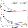 |
Fig. 1. Center-to-limb variation of the Ca I 4227 line-center fractional linear polarization Q/I (upper panel) and U/I (lower panel) obtained from CRD, PRD–AA, and PRD–AD calculations in the FAL-C atmospheric model, both in the absence (dotted curves) and in the presence (solid curves) of a magnetic field. The dotted curves for U/I are equal to zero. In the magnetic case, a height-independent horizontal (θB = π/2, χB = 0) magnetic field of 20 G is considered. The reference direction for positive Stokes Q is parallel to the y-axis of the considered reference system (i.e., perpendicular to the magnetic field). |
At the limb, the presence of a height-independent horizontal (θB = π/2, χB = 0) magnetic field of 20 G produces – via the Hanle effect – a depolarization and a rotation of the linear polarization plane. This leads to a decrease in the line-core Q/I peak while giving rise to an appreciable U/I signal (see solid curves). At the solar disk center, the forward-scattering Hanle effect yields a nonzero Q/I signal, while U/I is zero, consistently with the geometry of the problem. The CRD, PRD–AA, and PRD–AD calculations show significant differences for all μ in both Q/I and U/I, with the PRD–AD results always showing the largest signal. A very interesting finding is that the PRD–AD results for Q/I drift away from the others while approaching the disk center. At μ = 1, the PRD–AD signal is well above 1%, that is, one order of magnitude larger than in the PRD–AA and CRD cases. Moving from the limb to the disk center, the Q/I signal obtained from PRD–AA and PRD–AD calculations first decreases, reaches a minimum, and then increases, always remaining positive. On the contrary, in the CRD case, it shows a sign reversal at around μ ≈ 0.6 and then remains negative until μ = 1, with amplitudes always below 0.1% (see also Fig. 2). We note that the differences between PRD–AA and PRD–AD calculations in Fig. 1 are magnified by the artificial depolarization that is introduced by the AA approximation in the line core of Q/I and U/I for μ ≠ 1, both in the absence and presence of magnetic fields (see Janett et al. 2021a). To better visualize the impact of the different scattering modelings on the forward-scattering Hanle effect signal, Fig. 2 shows the emergent Q/I profiles at μ = 1. This clearly highlights the significantly stronger polarization signals resulting from PRD–AD calculations.
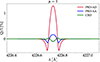 |
Fig. 2. Emergent Q/I profiles of Ca I 4227 at μ = 1, obtained from CRD, PRD–AA, and PRD–AD calculations in the FAL-C atmospheric model, in the presence of a height-independent horizontal (θB = π/2, χB = 0) magnetic field of 20 G. The reference direction for positive Stokes Q is parallel to the y-axis of the considered reference system (i.e., perpendicular to the magnetic field). In this geometry, the U/I profile vanishes, and is thus omitted. |
Figure 3 compares the polarization diagrams for the line-center radiation emitted at μ = 1 obtained with PRD–AD, PRD–AA, and CRD calculations, considering height-independent horizontal (i.e., θB = π/2) magnetic fields of 20 G with different azimuths χB. These diagrams further highlight the large polarization amplitudes of the forward-scattering Hanle effect signals obtained in the PRD–AD setting. We find differences of approximately one order of magnitude (in both Q/I and U/I) when comparing PRD–AD with PRD–AA and CRD results. Much smaller yet relevant differences are instead found between the CRD and PRD–AA calculations. Consistently with the geometry of the problem, Q/I and U/I vanish for χB = π/4 + n π/2 and χB = n π/2 (n = 0, ..., 3), respectively. We note that the evolution of the amplitudes of Q/I and U/I shows a counterclockwise rotation in all cases. Interestingly, the line-center signal provided by CRD calculations always has the opposite sign with respect to that provided by PRD–AA and PRD–AD calculations.
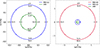 |
Fig. 3. Polarization diagrams of the Ca I 4227 line-center emergent radiation at μ = 1, obtained from CRD, PRD–AA, and PRD–AD calculations in the FAL-C atmospheric model, in the presence of a height-independent horizontal (θB = π/2) magnetic field of 20 G. The circular markers indicate the effective calculations, carried out for the azimuths χB = n π/8 (with n = 0, ..., 15). Left panel: Comparison between CRD and PRD–AA calculations. Right panel: Comparison between CRD, PRD–AA, and PRD–AD calculations (in the PRD–AA and CRD diagrams the circular marker indicates a magnetic field direction with azimuth χB = 0, whereas the arrow refers to χB = π/4). The reference direction for positive Stokes Q is parallel to the y-axis of the considered reference system. |
Figure 4 shows the line-center linear polarization degree,
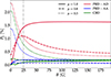 |
Fig. 4. Line-center linear polarization degree as a function of the strength of a horizontal (θB = π/2, χB = 0) magnetic field, obtained from PRD–AD (red), PRD–AA (blue), and CRD (green) calculations, for different LOSs. The vertical dash-dotted line indicates the Hanle critical field of Ca I 4227 (BH = 25 G). |
as a function of the strength of a horizontal (θB = π/2, χB = 0) magnetic field, for different LOSs, obtained from PRD–AD, PRD–AA, and CRD calculations. At the solar disk center (μ = 1, solid lines), where the polarization is fully produced by the forward-scattering Hanle effect, PL is already appreciable for magnetic fields of a few gauss only. Its value quickly grows as the magnetic field strength increases further, and finally stabilizes above the Hanle critical field. The increase in PL is much steeper and significant in the PRD–AD case than in the PRD–AA and CRD ones. Notably, the increase is not monotonic in the CRD case. As expected, for a near-limb LOS (μ = 0.3, dotted lines), the Hanle effect produces a monotonic decrease in PL with the magnetic field strength, until reaching a saturation regime. For an intermediate LOS (μ = 0.8, dashed lines), the value of PL first increases with the field strength, reaches a maximum, and then decreases until the saturation regime. In the PRD–AD case, the initial increase is much steeper and significant, and the maximum is reached for stronger fields (around the Hanle critical field) than in the other cases. The PRD–AD calculations show significantly larger values of PL for all LOSs and for any magnetic field strength.
3.2. Inclined magnetic fields
The results presented in the previous section are obtained considering horizontal magnetic fields. This geometry maximizes the breaking of the axial symmetry for a given value of B, and thus the amplitude of the polarization signals produced at the disk center via the forward-scattering Hanle effect. On the other hand, the discrepancies between the emergent Stokes profiles resulting from PRD–AD, PRD–AA, and CRD calculations change significantly if magnetic fields with different inclinations with respect to the vertical are considered. For this reason, we now analyze the case of a nonhorizontal inclined magnetic field. Figure 5 shows the center-to-limb variation of the amplitude of the line-center scattering polarization Q/I (upper panel) and U/I (lower panel) signals of the Ca I 4227 Å line resulting from PRD–AD, PRD–AA, and CRD calculations in the presence of a height-independent inclined (θB = π/4, χB = 0) magnetic field of 20 G. This setting confirms the presence of relevant differences between the different scattering descriptions for all μ, and in particular for the forward-scattering geometry (μ = 1). To better visualize the impact of the different scattering modelings on the forward-scattering Hanle effect signal, Fig. 6 shows the emergent Q/I and U/I profiles at μ = 1 for the same inclined magnetic field. Unlike in the case of a horizontal magnetic field shown in Fig. 2, this geometry produces an appreciable U/I signal. The significantly stronger linear polarization signals resulting from PRD–AD calculations are found both in Q/I and U/I.
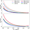 |
Fig. 5. Same as Fig. 1, but for a height-independent inclined (θB = π/4, χB = 0) magnetic field of 20 G. |
 |
Fig. 6. Same as Fig. 2, but for a height-independent inclined (θB = π/4, χB = 0) magnetic field of 20 G. |
Figure 7 compares the polarization diagrams for the line-center radiation emitted at μ = 1 obtained with PRD–AD, PRD–AA, and CRD calculations, considering height-independent inclined (i.e., θB = π/4) magnetic fields of 20 G with different azimuths χB. These diagrams reveal smaller forward-scattering signals than those presented in Fig. 3 due to the smaller horizontal component of the 20 G magnetic field. Moreover, both the CRD and PRD–AA diagrams are rotated with respect to the PRD–AD one. This means that both approximations could lead to the wrong sign being determined for the Q/I and U/I line-center signals. Figure 8 shows a similar polarization diagram, but for χB = 0 and different inclinations θB of the 20 G magnetic field. As expected, the Q/I and U/I signals vanish in the presence of a vertical magnetic field, that is θB = 0, π. As soon as the magnetic field is sufficiently inclined, the CRD and PRD–AA calculations significantly underestimate the amplitude of the line-center fractional linear polarization signals with respect to the PRD–AD modeling. Interestingly, the CRD diagram always shows negative line-center Q/I signals.
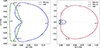 |
Fig. 8. Polarization diagrams obtained considering a height-independent magnetic field of 20 G with a fixed azimuth χB = 0, and varying its inclination θB ∈ [0, π]. The circular markers indicate the effective calculations, carried out for θB = n π/12 with n = 0, ..., 12. The other parameters are the same as in Fig. 3. |
4. Discussion
In general, CRD and PRD–AA calculations significantly underestimate the amplitude of the line-center fractional linear polarization signals with respect to the PRD–AD modeling, and even the sign can be wrong. Providing a simple and intuitive interpretation of these results is unfortunately not straightforward. Here, we provide a few qualitative insights.
The polarization properties of scattered radiation strongly depend on the detailed spectral and angular dependencies of the incident radiation field. These dependencies can only be fully taken into account through a PRD–AD description of scattering processes, while they are necessarily smoothed by the averages inherent to the PRD–AA and CRD approximations. Indeed, it can be shown that the CRD, PRD–AA, and PRD–AD calculations coincide in the limit of a spectrally flat and isotropic radiation field. It appears reasonable that scattering polarization signals, which are ultimately due to the geometry of the problem and symmetry-breaking effects, are enhanced by the PRD–AD approach, which exactly accounts for the complex coupling between the frequencies and propagation directions of the incoming and scattered radiation. In addition, the particular spectral structure and anisotropy of the solar radiation field depend on the thermal and density stratification of the atmospheric model through nonlocal RT effects. Inspecting and predicting these effects in nonacademic scenarios is notoriously difficult, and predicting how they are impacted by the considered approximations in the modeling of scattering processes is an even more complex task. In conclusion, it is not possible to clearly identify a single specific reason that explains the large differences observed between the CRD or PRD–AA calculations with respect to the general PRD–AD modeling. This further emphasizes the difficulty of predicting the suitability of the aforementioned approximations, and the need to quantitatively assess their accuracy through detailed calculations in the considered scenario. At the dawn of the new generation of big solar spectropolarimetric facilities, like the Daniel K. Inouye Solar Telescope (DKIST, Rimmele et al. 2020) and the future European Solar Telescope (EST, Quintero Noda et al. 2022), the need for an accurate modeling of the polarization of spectral lines is indeed stronger than ever before.
Finally, we comment on the significant discrepancies between the theoretical calculations presented in Sect. 3.1, which predict polarization signals of around 1%, and the observations of Bianda et al. (2011), which show signals one order of magnitude weaker (around 0.1%). We first note that a horizontal magnetic field maximizes the breaking of the axial symmetry and thus the forward-scattering Hanle effect. Although such a magnetic field would not be too unrealistic at 900 km, where the core of this line forms, it is important to bear in mind that we are assuming that the magnetic field is fully deterministic, and that we are neglecting 3D effects. As shown by Jaume Bestard et al. (2021), the presence of an inclined magnetic field reduces (and does not enhance) the amplitude of the scattering polarization signals produced by both horizontal inhomogeneities of the solar plasma and spatial gradients of the plasma bulk velocity (which are neglected in this 1D investigation). We also recall that the observations of Bianda et al. (2011) were performed in a relatively magnetized region, and that the impact of instrumental effects on the observed line-core signals is significant, especially in forward-scattering observations (e.g., Zeuner et al. 2020; del Pino Alemán & Trujillo Bueno 2021, for the Sr I 4607 Å line). Hence, the aforementioned discrepancies do not appear to be critical; however, it is clear that to reliably interpret observations of forward-scattering polarization signals, it is necessary to perform RT calculations in state-of-the-art 3D MHD atmospheric models, accounting for both magnetic and nonmagnetic symmetry-breaking effects (i.e., for both mechanisms (i) and (ii)).
5. Conclusions
The results of this work show that a reliable modeling of the fractional linear polarization signals produced through the forward-scattering Hanle effect in the Ca I line at 4227 Å requires PRD effects to be taken into account in their general AD formulation. If the CRD or PRD–AA approximations are considered, the amplitude of the line-center Q/I and U/I signals close to μ = 1 could be significantly underestimated, and even the sign could be wrong. This finding is of clear relevance, especially for the development of new methods for solar magnetic field diagnostics based on forward-scattering polarization signals in the Ca I 4227 Å line.
It can be expected that the results presented here for the Ca I 4227 Å line generalize to other strong resonance lines, for which PRD effects are relevant. For this reason, it is important to extend this work to other spectral lines of interest for Hanle diagnostics, such as those recently observed by the CLASP experiments (e.g., Kano et al. 2017; Rachmeler et al. 2022), or those that DKIST (and EST) will allow the observation of with unprecedented spatial and temporal resolution. At the same time, it will be interesting to investigate the same mechanism in lines pertaining to multiplets, or produced by elements with hyperfine structure.
Finally, it will be important to consider comprehensive 3D atmospheric models, which include horizontal inhomogeneities of the solar plasma and spatial gradients of the bulk velocity. In this respect, the first 3D NLTE RT calculations, taking scattering polarization and AD PRD effects into account, will soon be available thanks to recent software and algorithmic developments (see Benedusi et al. 2023).
Acknowledgments
The authors wish to thank the referee, for insightful comments that allowed improving the quality of the manuscript. This work was financed by the Swiss National Science Foundation (SNSF) through grant CRSII5_180238. T.P.A.’s participation in the publication is part of the Project RYC2021-034006-I, funded by MICIN/AEI/10.13039/501100011033, and the European Union “NextGeneration”/RTRP. T.P.A., J.T.B, and E.A.B. acknowledge support from the Agencia Estatal de Investigación del Ministerio de Ciencia, Innovación y Universidades (MCIU/AEI) under grant “Polarimetric Inference of Magnetic Fields” and the European Regional Development Fund (ERDF) with reference PID2022-136563NB-I00/10.13039/501100011033. J.Š. acknowledges the financial support from project RVO:67985815 of the Astronomical Institute of the Czech Academy of Sciences.
References
- Alsina Ballester, E., Belluzzi, L., & Trujillo Bueno, J. 2018, ApJ, 854, 150 [Google Scholar]
- Anusha, L. S., Nagendra, K. N., Bianda, M., et al. 2011, ApJ, 737, 95 [NASA ADS] [CrossRef] [Google Scholar]
- Benedusi, P., Janett, G., Belluzzi, L., & Krause, R. 2021, A&A, 655, A88 [NASA ADS] [CrossRef] [EDP Sciences] [Google Scholar]
- Benedusi, P., Janett, G., Riva, S., Krause, R., & Belluzzi, L. 2022, A&A, 664, A197 [NASA ADS] [CrossRef] [EDP Sciences] [Google Scholar]
- Benedusi, P., Riva, S., Zulian, P., et al. 2023, J. Comput. Phys., 479, 112013 [NASA ADS] [CrossRef] [Google Scholar]
- Bianda, M., Ramelli, R., Anusha, L. S., et al. 2011, A&A, 530, L13 [NASA ADS] [CrossRef] [EDP Sciences] [Google Scholar]
- Bommier, V. 1997a, A&A, 328, 726 [NASA ADS] [Google Scholar]
- Bommier, V. 1997b, A&A, 328, 706 [NASA ADS] [Google Scholar]
- Capozzi, E., Alsina Ballester, E., Belluzzi, L., et al. 2020, A&A, 641, A63 [NASA ADS] [CrossRef] [EDP Sciences] [Google Scholar]
- Carlin, E. S., & Bianda, M. 2016, ApJ, 831, L5 [NASA ADS] [CrossRef] [Google Scholar]
- Carlin, E. S., & Bianda, M. 2017, ApJ, 843, 64 [NASA ADS] [CrossRef] [Google Scholar]
- del Pino Alemán, T., & Trujillo Bueno, J. 2021, ApJ, 909, 180 [CrossRef] [Google Scholar]
- del Pino Alemán, T., Trujillo Bueno, J., Štěpán, J., & Shchukina, N. 2018, ApJ, 863, 164 [CrossRef] [Google Scholar]
- del Pino Alemán, T., Trujillo Bueno, J., Casini, R., & Manso Sainz, R. 2020, ApJ, 891, 91 [CrossRef] [Google Scholar]
- Faurobert, M. 1988, A&A, 194, 268 [NASA ADS] [Google Scholar]
- Fontenla, J. M., Avrett, E. H., & Loeser, R. 1993, ApJ, 406, 319 [Google Scholar]
- Gandorfer, A. 2000, The Second Solar Spectrum: A High Spectral Resolution Polarimetric Survey of Scattering Polarization at the Solar Limb in Graphical Representation, Vol. I: 4625 Å–6995 Å, (Zurich: vdf-ETH) [Google Scholar]
- Gandorfer, A. 2002, The Second Solar Spectrum: A High Spectral Resolution Polarimetric Survey of Scattering Polarization at the Solar Limb in Graphical Representation, Vol. II: 3910 Å–4630 Å, (Zurich: vdf-ETH) [Google Scholar]
- Gandorfer, A. 2005, The Second Solar Spectrum: A High Spectral Resolution Polarimetric Survey of Scattering Polarization at the Solar Limb in Graphical Representation, Vol. III: 3160 Å–3915 Å (Zurich: vdf-ETH) [Google Scholar]
- Guerreiro, N., Janett, G., Riva, S., Benedusi, P., & Belluzzi, L. 2024, A&A, 683, A207 [NASA ADS] [CrossRef] [EDP Sciences] [Google Scholar]
- Janett, G., Alsina Ballester, E., Guerreiro, N., et al. 2021a, A&A, 655, A13 [NASA ADS] [CrossRef] [EDP Sciences] [Google Scholar]
- Janett, G., Benedusi, P., Belluzzi, L., & Krause, R. 2021b, A&A, 655, A87 [NASA ADS] [CrossRef] [EDP Sciences] [Google Scholar]
- Janett, G., Benedusi, P., & Riva, F. 2024, A&A, 682, A68 [NASA ADS] [CrossRef] [EDP Sciences] [Google Scholar]
- Jaume Bestard, J., Trujillo Bueno, J., Štěpán, J., & del Pino Alemán, T. 2021, ApJ, 909, 183 [NASA ADS] [CrossRef] [Google Scholar]
- Kano, R., Trujillo Bueno, J., Winebarger, A., et al. 2017, ApJ, 839, L10 [NASA ADS] [CrossRef] [Google Scholar]
- Landi Degl’Innocenti, E., & Landolfi, M. 2004, Polarization in Spectral Lines, ASSL, (Dordrecht: Kluwer), 307 [CrossRef] [Google Scholar]
- Manso Sainz, R., & Trujillo Bueno, J. 2011, ApJ, 743, 12 [NASA ADS] [CrossRef] [Google Scholar]
- Quintero Noda, C., Schlichenmaier, R., Bellot Rubio, L. R., et al. 2022, A&A, 666, A21 [NASA ADS] [CrossRef] [EDP Sciences] [Google Scholar]
- Rachmeler, L. A., Trujillo Bueno, J., McKenzie, D. E., et al. 2022, ApJ, 936, 67 [NASA ADS] [CrossRef] [Google Scholar]
- Ramelli, R., Balemi, S., Bianda, M., et al. 2010, Proc. SPIE, 7735, 77351Y [Google Scholar]
- Rimmele, T. R., Warner, M., Keil, S. L., et al. 2020, Sol. Phys., 295, 172 [Google Scholar]
- Riva, F., Janett, G., & Belluzzi, L. 2024, A&A, 688, A10 [NASA ADS] [CrossRef] [EDP Sciences] [Google Scholar]
- Riva, S., Guerreiro, N., Janett, G., et al. 2023, A&A, 679, A87 [NASA ADS] [CrossRef] [EDP Sciences] [Google Scholar]
- Sampoorna, M., Trujillo Bueno, J., & Landi Degl’Innocenti, E. 2010, ApJ, 722, 1269 [NASA ADS] [CrossRef] [Google Scholar]
- Sampoorna, M., Nagendra, K. N., & Stenflo, J. O. 2017, ApJ, 844, 97 [NASA ADS] [CrossRef] [Google Scholar]
- Stenflo, J. O. 2003, ASP Conf. Ser., 307, 385 [NASA ADS] [Google Scholar]
- Stenflo, J. O., & Keller, C. U. 1997, A&A, 321, 927 [NASA ADS] [Google Scholar]
- Trujillo Bueno, J. 2001, ASP Conf. Ser., 236, 161 [Google Scholar]
- Trujillo Bueno, J., & del Pino Alemán, T. 2022, ARA&A, 60, 415 [NASA ADS] [CrossRef] [Google Scholar]
- Trujillo Bueno, J., Landi Degl’Innocenti, E., Collados, M., Merenda, L., & Manso Sainz, R. 2002, Nature, 415, 403 [Google Scholar]
- Uitenbroek, H. 2001, ApJ, 557, 389 [Google Scholar]
- Štěpán, J., & Trujillo Bueno, J. 2013, A&A, 557, A143 [NASA ADS] [CrossRef] [EDP Sciences] [Google Scholar]
- Štěpán, J., & Trujillo Bueno, J. 2016, ApJ, 826, L10 [Google Scholar]
- Zeuner, F., Manso Sainz, R., Feller, A., et al. 2020, ApJ, 893, L44 [NASA ADS] [CrossRef] [Google Scholar]
All Figures
|
Fig. 1. Center-to-limb variation of the Ca I 4227 line-center fractional linear polarization Q/I (upper panel) and U/I (lower panel) obtained from CRD, PRD–AA, and PRD–AD calculations in the FAL-C atmospheric model, both in the absence (dotted curves) and in the presence (solid curves) of a magnetic field. The dotted curves for U/I are equal to zero. In the magnetic case, a height-independent horizontal (θB = π/2, χB = 0) magnetic field of 20 G is considered. The reference direction for positive Stokes Q is parallel to the y-axis of the considered reference system (i.e., perpendicular to the magnetic field). |
| In the text | |
|
Fig. 2. Emergent Q/I profiles of Ca I 4227 at μ = 1, obtained from CRD, PRD–AA, and PRD–AD calculations in the FAL-C atmospheric model, in the presence of a height-independent horizontal (θB = π/2, χB = 0) magnetic field of 20 G. The reference direction for positive Stokes Q is parallel to the y-axis of the considered reference system (i.e., perpendicular to the magnetic field). In this geometry, the U/I profile vanishes, and is thus omitted. |
| In the text | |
|
Fig. 3. Polarization diagrams of the Ca I 4227 line-center emergent radiation at μ = 1, obtained from CRD, PRD–AA, and PRD–AD calculations in the FAL-C atmospheric model, in the presence of a height-independent horizontal (θB = π/2) magnetic field of 20 G. The circular markers indicate the effective calculations, carried out for the azimuths χB = n π/8 (with n = 0, ..., 15). Left panel: Comparison between CRD and PRD–AA calculations. Right panel: Comparison between CRD, PRD–AA, and PRD–AD calculations (in the PRD–AA and CRD diagrams the circular marker indicates a magnetic field direction with azimuth χB = 0, whereas the arrow refers to χB = π/4). The reference direction for positive Stokes Q is parallel to the y-axis of the considered reference system. |
| In the text | |
|
Fig. 4. Line-center linear polarization degree as a function of the strength of a horizontal (θB = π/2, χB = 0) magnetic field, obtained from PRD–AD (red), PRD–AA (blue), and CRD (green) calculations, for different LOSs. The vertical dash-dotted line indicates the Hanle critical field of Ca I 4227 (BH = 25 G). |
| In the text | |
|
Fig. 5. Same as Fig. 1, but for a height-independent inclined (θB = π/4, χB = 0) magnetic field of 20 G. |
| In the text | |
|
Fig. 6. Same as Fig. 2, but for a height-independent inclined (θB = π/4, χB = 0) magnetic field of 20 G. |
| In the text | |
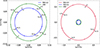 |
Fig. 7. Same as Fig. 3, but for a height-independent inclined (θB = π/4) magnetic field of 20 G. |
| In the text | |
|
Fig. 8. Polarization diagrams obtained considering a height-independent magnetic field of 20 G with a fixed azimuth χB = 0, and varying its inclination θB ∈ [0, π]. The circular markers indicate the effective calculations, carried out for θB = n π/12 with n = 0, ..., 12. The other parameters are the same as in Fig. 3. |
| In the text | |
Current usage metrics show cumulative count of Article Views (full-text article views including HTML views, PDF and ePub downloads, according to the available data) and Abstracts Views on Vision4Press platform.
Data correspond to usage on the plateform after 2015. The current usage metrics is available 48-96 hours after online publication and is updated daily on week days.
Initial download of the metrics may take a while.