| Issue |
A&A
Volume 687, July 2024
|
|
|---|---|---|
| Article Number | A249 | |
| Number of page(s) | 6 | |
| Section | The Sun and the Heliosphere | |
| DOI | https://doi.org/10.1051/0004-6361/202449772 | |
| Published online | 17 July 2024 | |
Large-amplitude transverse MHD waves prevailing in the Hα chromosphere of a solar quiet region revealed by MiHI integrated field spectral observations
1
Astronomy Program, Department of Physics and Astronomy, Seoul National University, Gwanak-gu, Seoul 08826, Korea
e-mail: jcchae@snu.ac.kr
2
Max-Planck Institute for Solar System Research, Justus-von-Liebig-Weg 3, 37077 Göttingen, Germany
3
Space Research and Technology Institute, Bulgarian Academy of Sciences, Acad. Georgy Bonchev Str., Bl. 1, 1113 Sofia, Bulgaria
4
Bay Area Environmental Research Institute, NASA Research Park, Moffett Field, CA 94035, USA
5
Lockheed Martin Solar & Astrophysics Laboratory, 3251 Hanover Street Palo Alto, CA 94304, USA
Received:
28
February
2024
Accepted:
6
May
2024
The investigation of plasma motions in the solar chromosphere is crucial for understanding the transport of mechanical energy from the interior of the Sun to the outer atmosphere and into interplanetary space. We report the finding of large-amplitude oscillatory transverse motions prevailing in the non-spicular Hα chromosphere of a small quiet region near the solar disk center. The observation was carried out on 2018 August 25 with the Microlensed Hyperspectral Imager (MiHI) installed as an extension to the spectrograph at the Swedish Solar Telescope (SST). MiHI produced high-resolution Stokes spectra of the Hα line over a two-dimensional array of points (sampled every 0.066″ on the image plane) every 1.33 s for about 17 min. We extracted the Doppler-shift-insensitive intensity data of the line core by applying a bisector fit to Stoke I line profiles. From our time–distance analysis of the intensity data, we find a variety of transverse motions with velocity amplitudes of up to 40 km s−1 in fan fibrils and tiny filaments. In particular, in the fan fibrils, large-amplitude transverse MHD waves were seen to occur with a mean velocity amplitude of 25 km s−1 and a mean period of 5.8 min, propagating at a speed of 40 km s−1. These waves are nonlinear and display group behavior. We estimate the wave energy flux in the upper chromosphere at 3 × 10⁶ erg cm−2 s−1. Our results contribute to the advancement of our understanding of the properties of transverse MHD waves in the solar chromosphere.
Key words: magnetohydrodynamics (MHD) / waves / Sun: atmosphere / Sun: chromosphere / Sun: corona
© The Authors 2024
 Open Access article, published by EDP Sciences, under the terms of the Creative Commons Attribution License (https://creativecommons.org/licenses/by/4.0), which permits unrestricted use, distribution, and reproduction in any medium, provided the original work is properly cited.
This article is published in open access under the Subscribe to Open model. Subscribe to A&A to support open access publication.
1. Introduction
Transverse magnetohydrodynamic (MHD) waves, such as Alfvén waves, have been regarded as one of the potential ways of transporting the mechanical energy required for coronal heating and solar wind acceleration (e.g.,Alfvén 1947; Alazraki & Couturier 1971). An important point is that if transverse waves are to be fully in charge of the coronal heating and the solar wind acceleration, they should have large velocity amplitudes in the photosphere and chromosphere, because the transmission efficiency of the waves in the solar atmosphere is very low due to the rapid increase in Alfvén speed with height (e.g.,Velli 1993). According to the recent theoretical study of Chae & Lee (2023), the velocity amplitude has to be as large as 20 km s−1 in the upper chromosphere, both in coronal holes and in active regions. This kind of theoretical consideration has motivated researchers to search for large-amplitude transverse waves in the chromosphere.
The transverse waves detected in the chromosphere of active regions so far are found to have velocity amplitudes much smaller than 20 km s−1. These values were mostly determined from observations of superpenumbral fibrils around sunspots. The values determined from transverse displacements are typically 1 km s−1 (Pietarila et al. 2011), with a mean of 0.8 km s−1 (Morton et al. 2021), and those determined from the analysis of a Doppler velocity pattern ranged from 0.6 to 1 km s−1 (Chae et al. 2021, 2022).
In contrast, the transverse waves in quiet regions are found to have large velocity amplitudes. The observations of spicules above the solar limb taken with the Solar Optical Telescope on board Hinode revealed large-amplitude transverse oscillations of spicules with number distributions of velocity amplitude displaying tails extending up to 30 km s−1 (De Pontieu et al. 2007; Okamoto & De Pontieu 2011; Pereira et al. 2012; Bate et al. 2022). From off-limb observations, it was also found that velocity amplitudes increase with height above the solar limb, with the mean value ranging from 18 km s−1 at 4900 km to 26 km s−1 at 7500 km (Bate et al. 2022). Transverse waves were also reported from the disk counterpart of limb spicules, that is, fibrils around strong network elements. Jess et al. (2009) found torsional oscillations with a velocity amplitude of 2.6 km s−1 at network bright points that may correspond to spicule footpoints. From their observations of on-disk spicules, Jess et al. (2012) reported transverse velocities with a mean of around 15 km s−1 and reaching up to 28 km s−1. Srivastava et al. (2017) reported high-frequency transverse oscillations with velocity amplitudes of 14 km s−1 from the observation of on-disk spicules. Observations of rapid blue excursions (RBEs), the supposed disk counterpart of Type II spicules, revealed transverse velocities with a mean amplitude of around 12 km s−1 (Sekse et al. 2013), reaching up to 22 km s−1 (Kuridze et al. 2015). All of these studies seem to support the notion that spicules carry transverse MHD waves with sufficiently large velocity amplitudes for coronal heating in quiet Sun regions.
We note, however, that spicules are not all plasma structures in the upper chromosphere of quiet regions. Spicules usually refer to plasma jets along the magnetic field lines that emanate from strong network magnetic elements, and become predominantly vertical at large heights. The disk counterparts of spicules were regarded as plasma structures that were called mottles or bushes in the past, and are presently often referred to as fibrils. In the past, however, the term “fibril” was used to refer to plasma structures that are supported by highly inclined magnetic field lines either in active or quiet regions of the solar atmosphere (Foukal 1971b). Among nonspicular elongated plasma structures are also threads (or loops), plasma structures connecting two magnetic poles of opposite polarity, and filaments, plasma structures located above the polarity inversion line. It is generally considered that all spicules, mottles, fibrils, threads, and filament fine structures trace local field lines in the chromosphere (Foukal 1971a), despite some exceptions reported from numerical modeling (Martínez-Sykora et al. 2016) or from spectropolarimetric observations (Asensio Ramos et al. 2017).
Observations of transverse waves in the nonspicular chromosphere of the quiet Sun are scarce. Morton et al. (2012) and Morton et al. (2013) are among the few authors to have reported such rare observations. They found transverse oscillations with mean velocity amplitudes of 6.4 km s−1 and 4.5 km s−1 in nonspicular fibrils, respectively. Very recently, Kwak et al. (2023) reported transverse oscillations in the line-of-light direction with a mean velocity amplitude of 1.3 km s−1 in quiet region fibrils that would be better referred to as chromospheric threads or loops.
In this paper, we report results from observations carried out with an integral field spectrograph covering a very small quiet region on the solar disk with a nearly diffraction limited resolution (0.12″), a high cadence (1.33 s), and a spectral resolution of R > 300 000, covering a wavelength range of 4.5 Å (±100 km s−1). The Hα chromosphere of the observed region happened to contain a number of fibrils and tiny filaments supported by predominantly horizontal magnetic fields. We found a variety of oscillatory transverse motions with mean velocity amplitudes of 9 km s−1, 25 km s−1, and 37 km s−1 in different groups. This is the first report on large-amplitude transverse oscillations prevailing in the nonspicular chromosphere of the quiet Sun.
2. Data and analysis
We used the Hα spectral data taken from a quiet region of the Sun on 2018 August 25 with the Microlensed Hyperspectral Imager (MiHI) prototype (van Noort et al. 2022; van Noort & Chanumolu 2022). The MiHI is an integral field spectrograph based on a double-sided microlens array (MLA) that was installed as an extension to the TRI-Port Polarimetric Echelle-Littrow (TRIPPEL) spectrograph at the Swedish Solar Telescope (SST). For information on the observed region, we use a photospheric magnetogram taken by the Heliospheric and Magnetic Imager (HMI) and images taken by the Atmospheric Imaging Assembly (AIA) on board the Solar Dynamics Observatory (SDO). The subregion of the HMI magnetograms that has a field of view (FOV) much larger than that of the MiHI was used to calculate potential magnetic fields in the chromosphere and corona. The AIA images sample emission at coronal (AIA 171 Å), transition region (AIA 304 Å), and chromospheric (AIA 1700 Å) temperatures.
The MiHI observations started at 09:07:48 UT and lasted for 1037 s, with a cadence of 1.33 s per frame. The FOV was 9.2″ × 8.2″ (6700 km by 6000 km) and the spatial sampling was 0.066″ (48 km). The conversion of the raw data frames to hyperspectral cubes and their restoration to high-resolution science-ready Stokes data was done following the data reduction procedure described by van Noort & Doerr (2022).
Every pixel contains the spectral profile covering 4.5 Å around the Hα line with sampling of 0.01 Å. We note that the spectral data were taken simultaneously at all the pixels without any time difference, as the MiHI is an integral field spectrograph. The data reduction process consists of bad-pixel mending, wavelength recalibration, telluric-line removal, and noise suppression based on the principal component analysis. The line intensity at every wavelength is expressed in units of continuum intensity, which is assumed to be equal to 1.18 times the offband intensity at −1.5 Å averaged over the FOV and over the observing time.
We obtained the core intensity and Doppler shift of the Hα line by applying a 0.5 Å width bisector fit to every line profile. The Doppler velocities are found to have a significantly large variation with a standard deviation of 4.1 km s−1. In principle, the combination of plane-of-sky transverse motion and line-of-sight Doppler motion should provide more information on oscillations and waves. However, the pattern of Doppler motion is found to be too complex for straightforward analysis. Moreover, in order to infer the line-of-sight motion of a feature that is overlapped by other structures along the line of sight, a sophisticated spectral analysis other than the simple bisector method is required, which is far beyond the scope of this work.
In the present work, we focus on the inference of transverse motion from the core intensity images. We note that the core intensity data were obtained from the spectral analysis, and are therefore insensitive to Doppler shifts. The core intensity is rather related to the Hα line source function S and optical thickness τ of the observed feature. We note that the Hα line source function S is constant over the wavelength to a good approximation. It is also commonly assumed that S is constant over the position along the line of sight. The equation of radiative transfer along the line of sight can then be solved to yield the expression

given in terms of background core intensity I0 and optical thickness τ as well as S. This expression is reduced to ΔI = S − I0 in the limit τ ≫ 1, and to ΔI = (S − I0)τ in the limit τ ≪ 1. We note that all S, I0, and τ are now functions of time and position on the image plane. In this study, as an approximation, we identify I0 with the slow-varying pattern that is constructed from the low-order polynomial fit of the temporal variation of the intensity at every position.
3. Results
Figure 1 shows the quiet region observed by MiHI as marked on SDO/AIA images and SDO/HMI magnetogram. This region does not show any noticeable bright coronal feature as seen in these images apart from faint small-scale loops. The HMI magnetogram indicates that the MiHI FOV contains one magnetic field concentration of positive polarity with a flux density of up to 90 G. We therefore conclude that the observed region was very quiet in the extreme ultraviolet (EUV)) and magnetograph observations during the MiHI observation and may be typical of quiet regions on the Sun. This implies that any process we observe in this FOV may not be particular to this region, but rather commonly occurring in other regions of the quiet Sun as well.
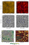 |
Fig. 1. Images of the observed region. a, b, c: context SDO/AIA images. d: SDO/HMI magnetogram. The blue rectangle indicates the 55″ × 51″ FOV of the submagnetogram below. e: SDO/HMI submagnetogram rotated to match the MiHI image frame where the origin is located in the lower left corner of the 9.2″ × 8.2″ MiHI FOV (red rectangle). The colored curves denote the projected magnetic field lines of the constructed potential field configuration with color representing height above the surface. f: MiHI Hα intensity image with the projected field lines superimposed. Most of these field lines inside the MiHI FOV have heights of < 4000 km. |
Figure 2 illustrates the Hα core intensity image of the observed region taken at one particular instant. The figure shows a number of elongated absorption structures. We find from the time series of the core intensity images that these structures change ceaselessly, even over just 17 min. A variety of motions occur in this small region in such a short time, including transverse motions perpendicular to the length, longitudinal motions, and large-scale rotating motions leading to the reorganization of the structures themselves. Here we focus on the time–distance (t − d) analysis of transverse motions perpendicular to the length.
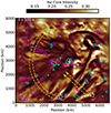 |
Fig. 2. Hα core intensity map taken at 500 s after the start of observations. The dashed arrows indicate the two main slits (FIL and ARC) and the two auxiliary slits (FIL2 and ARC2). The cyan-colored and magenta-colored contours represent ±1σ levels of offband intensity at −1.5 Å, and the plus symbol marks the center of the offband bright concentration co-spatial with the magnetic concentration of positive polarity. |
There are two categories of absorption structures in our observation: fan fibrils and tiny filaments. The fan fibrils are lower-contrast features comprising a fan structure extending approximately radially outward from the positive magnetic concentration inside the MiHI FOV. These fibrils are likely to be supported by highly horizontal, low-lying magnetic field lines connecting this magnetic concentration and some magnetic concentrations of negative polarity outside the MiHI FOV. The constructed potential magnetic fields demonstrate the existence of these field lines. The potential field lines are fairly horizontal, and are mostly located at heights of 2000–4000 km (see Fig. 1f). The field strength at the loop tops at these heights is estimated at around 10 G. It is not surprising to find some misalignments between the fibrils and the potential field lines, because the effects of plasma pressure and gravitational force may not be negligible in the chromosphere. If these effects were taken into account, the field lines would become flatter, and the magnetic field strength would then be a little higher than 10 G. For the study of the transverse motions in these fan fibrils, we define the arc-shaped slits ARC and ARC2 for the t − d analysis, as shown in Fig. 1.
The tiny filaments are higher-contrast absorption structures outside the fan structure. These structures do not originate from the magnetic concentration, and are not aligned with the constructed potential fields (see Fig. 1f). It seems that these features are supported by highly nonpotential and predominantly horizontal magnetic fields. This is one reason why we identify them as filaments. For the study of transverse motion in these filaments, we define the two straight slits FIL and FIL2 for the t − d analysis.
We find a variety of large-amplitude velocity oscillations in this region. We categorize the transverse oscillatory motions into three groups; those with velocity amplitudes V < 15 km s−1 (Group I), those with 20 < V < 30 km s−1 (Group II), and those with V > 30 km s−1 (Group III). Group I oscillations occurred continually in the filaments, and the Group II oscillations prevailed in the fan fibrils for about 350 s among the observing duration of 1037 s. Group III oscillations occurred from time to time in the fan fibrils, less frequently than the oscillations in the other groups.
Transverse oscillations belonging to Group I occur mostly in the filaments, and are easily identified from the t − d map of intensity constructed along the slit FIL shown in Fig. 3. These fibrils are characterized by contrast ΔI ∼ −0.06 and a full width at half maximum (FWHM) of w ∼ 200 km (see Table 1). In Fig. 4, we mark line segments representing our manual tracing of some noticeable displacements of the filaments. The slope of each line segment yields the instantaneous velocity at a particular instant; these range from 6 to 9 km s−1. These instantaneous motions are parts of an oscillatory motion, and the velocity amplitude of the oscillatory motion is larger than or equal to any measured instantaneous speed. To determine the velocity amplitude and period of each oscillatory motion, we manually traced the oscillatory motion by drawing on the t − d map a sinusoidal curve of the form d = Dsin(2π(t − t0)/P) that best matches the pattern of the oscillatory displacement. As a result, we found oscillations (FIL:1,2,3, 4) with periods P of 120–130 s, and velocity amplitudes of V ≡ 2πD/P of 7–11 km s−1 as listed in Table 1. An oscillation in Group I was also identified in one of the fan fibrils from the t − d map constructed along the slit ARC shown in Fig. 4. This oscillation (ARC: 1) has a velocity amplitude of 11 km s−1, which is comparable to those of FIL: 1–4, and has a period of 260 s, which is longer than those seen at the slit FIL.
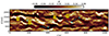 |
Fig. 3. Time–distance ΔI map constructed along the slit FIL. Each cyan-colored dashed line segment traces the trajectory of a filament at each instant, and its slope corresponds to the instantaneous velocity at one particular instant, as explicitly specified by a cyan-colored number (in units of km s−1). Each red sinusoidal curve traces the transverse oscillation of the filament, which is indexed by red numbers ranging from 1 to 4. |
Inferred values of the period P and velocity amplitude V of the transverse oscillations, and the intensity difference ΔI (in units of continuum intensity), and the FWHM width w of the fibrils and filaments.
Figure 4 shows the transverse oscillations in Groups II and III as well. The transverse oscillations (ARC: 5–8) in Group II are distinct from those in Group I in several ways. First, unlike those in Group I, the trajectories of the Group II oscillations are not uniform, either in intensity or in width, and appear fragmented at certain instances. This kind of trajectory fragmentation might be because short fibrils move in and out of the slit along the fibril length. We manually drew the sinusoidal curves to approximate the fragmented trajectories as shown in the figure. We believe that these curves, though imprecise, reasonably characterize the oscillatory transverse motions. The probable errors in the determination of D are responsible for most of the probable errors in V, which are estimated to be about 2 km s−1 in three oscillations (ARC: 5, 6, 8) and about 8 km s−1 in the other oscillation (ARC: 7). We find that these oscillations are characterized by larger velocity amplitudes (from 24 to 27 km s−1) and longer periods (320–380 s) than those in Group I (see Table 1).
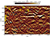 |
Fig. 4. Time–distance ΔI map constructed along the slit ARC. Each cyan-colored dashed line segment traces the trajectory of a fibril at each instant, and its slope corresponds to the instantaneous velocity at one particular instant, as explicitly specified by a cyan-colored number (in unit of km s−1). Each red sinusoidal curve traces the transverse oscillation of a fibril, which is indexed by red numbers ranging from 1 to 8. |
An important property of the transverse oscillations in Group II (ARC: 5–8) is the group behavior. These oscillations are not independent of one another; they have similar phases, periods, and amplitudes, even though they occurred at different locations on the cut ARC. The consistency in these four oscillations strongly suggests that they may have originated from the same source.
The transverse oscillations (ARC: 2–4) in Group III are characterized by very large velocity amplitudes, above 30 km s−1, and short periods of about 160 s. The trajectories are regular, but the identified durations are much shorter than the period. The fibrils displaying these oscillations are less dark (ΔI ∼ −0.02) and are thinner (w ∼ 140 km) than those in Group I. These fibrils seem to appear at higher altitudes. It is noteworthy that the periods and widths of the quiet Sun features summarized in Table 1 are comparable with the reported lifetimes and widths of dynamic fibrils in active regions (e.g., Tsiropoula et al. 2012).
Finally, in addition to the transverse oscillations, the t − d map in Fig. 4 displays a number of short-lived (< 60 s) transverse motions as inferred from the faint intensity streaks (marked by dashed line segments). Their slopes correspond to speeds from 6 to 29 km s−1. As these speeds are in the same range as the oscillatory motions examined above, these streaks are probably of the same kind as the oscillatory motions.
Now we attempt to determine the propagation speed of the transverse oscillations. For the transverse oscillations in Group I, we constructed another time–distance map along the slit FIL2, which is parallel to FIL and is 240 km away from it (lower left from FIL). The time lags obtained from the transverse motions of FIL: 1, 3, and 4 are about 4 s. This means that the oscillations propagate along the filaments at a speed of about 60 km s−1. For the oscillations in fan fibrils, we constructed another t − d map along the slit ARC2, which is parallel to ARC but has a smaller radius, with the distance between the two slits being 240 km. From the transverse oscillation ARC: 6 in Group II, we roughly estimate the time lag at about +6 s, which corresponds to a speed of about 40 km s−1. For the transverse oscillations in Group III, we obtained a time lag of about −5 s, corresponding to a velocity of −48 km s−1. The inward waves implied by the negative velocity might have originated either from wave excitation at a remote magnetic concentration of negative polarity or from wave reflection at a place where the gradient of the Alfvén speed is large (e.g., Velli 1993). The propagation speeds inferred here are quite compatible with the theoretical range of Alfvén speed, 15 to 91 km s−1, in the upper chromosphere of the quiet Sun obtained with the field strength of 10 G, and the range of mass density from 3.5 × 10⁻¹² g cm−3 to 9.5 × 10⁻¹⁴ g cm−3 taken from an atmospheric model of the quiet Sun (Fontenla et al. 1993). This supports the idea that the observed transverse oscillations represent transverse MHD waves propagating at speeds comparable to the Alfvén speed in the upper chromosphere.
4. Discussion
In the present work we report the observation of a small region on the Sun that appears to be highly typical of the quiet Sun. The Hα chromosphere of this region contains two kinds of elongated absorption structures: fan fibrils supported by highly horizontal magnetic fields and tiny filaments supported by nonpotential magnetic fields. The Hα spectral observations of high angular resolution and high temporal resolution obtained with the MiHI prototype reveal that this region was very dynamic, displaying a variety of transverse motions with velocity amplitudes of up to 40 km s−1. Interestingly, however, no noticeable activities were seen in the EUV image data.
Particularly important is our finding of large-amplitude transverse oscillations in fan fibrils (Group II oscillations). The velocity amplitudes of these oscillations have a mean value of about 25 km s−1. We note that such mean velocity amplitudes were previously only reported from observations of spicules seen high above the limb; for example, 7500 km above the limb (Bate et al. 2022). Our study is the first to report a large mean value of velocity amplitudes obtained from on-disk observations of the nonspicular chromosphere at low heights < 4000 km.
We now consider our estimates of the wave energy flux in the chromosphere and corona. We estimate the Alfvén wave energy flux in the chromosphere at 2.8 × 10⁶ erg cm−2 s−1 from the observed mean velocity amplitude of 25 km s−1 and the magnetic field strength of 10 G; for these estimates, we adopted a mass density of 1.0 × 10⁻¹³ g cm−3. Furthermore, by multiplying the theoretical transmission of 0.36 (Chae & Lee 2023), we estimate the wave energy flux in the corona at 9.5 × 10⁵ erg cm−2 s−1. This estimate is comparable to the wave flux of 8.0 × 10⁵ erg cm−2 s−1 required for coronal heating and solar wind acceleration in corona hole regions (Chae & Lee 2023). Contrary to our expectations, we did not detect any noticeable activity in the coronal image data, despite the occurrence of the large-amplitude transverse waves in the fan fibrils. This could be explained by the fact that the guiding magnetic field lines are strongly inclined to the horizontal, forming low-lying magnetic loops that are not directly connected to the corona above, unlike the spicular chromosphere. Nevertheless, the transverse waves may still contribute to the heating of these low-lying magnetic loops. Moreover, it would be natural to suppose that large-amplitude transverse waves as observed in the fan fibrils take place also in the spicular chromosphere, contributing much to the coronal heating and solar wind acceleration.
We note that the transverse MHD waves we observed not only have large velocity amplitudes, but are also significantly nonlinear. The nonlinearity of these waves is indicated by the large value of the observed mean velocity amplitude 25 km s−1 in comparison with the estimated propagation speed of 40 km s−1. It is well known from theoretical studies (Hollweg et al. 1982; Kudoh & Shibata 1999) that nonlinear Alfvén waves are coupled with compressible waves; these Alfvén waves excite longitudinal motions that propagate as slow or fast waves and develop into shock waves. This kind of nonlinear coupling seems to be consistent with the properties of the oscillations we observed in Group II. The variations of intensity and width in the trajectories may be attributed to the co-existence with compressible waves as in the previous studies (Jess et al. 2012; Morton et al. 2012; Sharma et al. 2018), and the fragmented appearance may be due to the presence of oscillatory longitudinal motions in and out of the slit.
It is also interesting that the transverse oscillations in Group II display group behavior. The transverse oscillations occurring in different fibrils have similar phases, velocity amplitudes (typically 25 km s−1), and periods (5–7 min). This group behavior may provide us with a clue as to the excitation process of the waves. These oscillations may have originated from the magnetic concentration where the magnetic field lines supporting the fibrils are rooted together. If the magnetic concentration is disturbed either by a linear motion or a twisting motion near the photosphere or below it, transverse velocity oscillations will be produced. These oscillations propagate simultaneously along different field lines, developing into transverse oscillations of different fibrils, and displaying the group behavior. In this regard, the observed group behavior is not strange, and may be a very natural property of fan fibrils. This property is not limited to fibrils of this kind, but may also appear in the spicules that emanate from the same magnetic concentration, which may be identified as torsional Alfvén waves (Srivastava et al. 2017).
In summary, our results indicate that large-amplitude transverse waves occur not only in the spicular chromosphere at large heights but also in the nonspicular chromosphere at small heights. The interesting properties (nonlinearity and group behavior) of the transverse waves in fan fibrils merit further systematic investigation based on the rigorous analysis of Doppler velocity data. Together with the previously reported results on transverse waves in the spicular chromosphere, our results contribute to the advancement of our understanding of the properties and excitation of transverse MHD waves in the Hα chromosphere of the quiet Sun.
Acknowledgments
We appreciate the referee’s critical comments that helped in our assessment of the scientific significance of this work. J.C. is grateful to Sami Solanki for the travel support and Hans-Peter Doerr for the hospitality provided during his visit to MPS in the summer of 2023. This work was supported by the National Research Foundation of Korea (RS-2023-00208117) and (RS-2023-00273679). M.M. acknowledges DFG grants WI 3211/8-1 and 3211/8-2, project number 452856778. The Swedish 1-m Solar Telescope is operated on the island of La Palma by the Institute for Solar Physics of Stockholm University in the Spanish Observatorio del Roque de los Muchachos of the Instituto de Astrofísica de Canarias. The Institute for Solar Physics is supported by a grant for research infrastructures of national importance from the Swedish Research Council (registration number 2021-00169).
References
- Alazraki, G., & Couturier, P. 1971, A&A, 13, 380 [NASA ADS] [Google Scholar]
- Alfvén, H. 1947, MNRAS, 107, 211 [CrossRef] [Google Scholar]
- Asensio Ramos, A., de la Cruz Rodríguez, J., Martínez González, M. J., & Socas-Navarro, H. 2017, A&A, 599, A133 [NASA ADS] [CrossRef] [EDP Sciences] [Google Scholar]
- Bate, W., Jess, D. B., Nakariakov, V. M., et al. 2022, ApJ, 930, 129 [NASA ADS] [CrossRef] [Google Scholar]
- Chae, J., & Lee, K.-S. 2023, ApJ, 954, 45 [NASA ADS] [CrossRef] [Google Scholar]
- Chae, J., Cho, K., Nakariakov, V. M., Cho, K.-S., & Kwon, R.-Y. 2021, ApJ, 914, L16 [NASA ADS] [CrossRef] [Google Scholar]
- Chae, J., Cho, K., Lim, E.-K., & Kang, J. 2022, ApJ, 933, 108 [CrossRef] [Google Scholar]
- De Pontieu, B., McIntosh, S. W., Carlsson, M., et al. 2007, Science, 318, 1574 [Google Scholar]
- Fontenla, J. M., Avrett, E. H., & Loeser, R. 1993, ApJ, 406, 319 [Google Scholar]
- Foukal, P. 1971a, Sol. Phys., 20, 298 [NASA ADS] [CrossRef] [Google Scholar]
- Foukal, P. 1971b, Sol. Phys., 19, 59 [NASA ADS] [CrossRef] [Google Scholar]
- Hollweg, J. V., Jackson, S., & Galloway, D. 1982, Sol. Phys., 75, 35 [NASA ADS] [CrossRef] [Google Scholar]
- Jess, D. B., Mathioudakis, M., Erdélyi, R., et al. 2009, Science, 323, 1582 [Google Scholar]
- Jess, D. B., Pascoe, D. J., Christian, D. J., et al. 2012, ApJ, 744, L5 [NASA ADS] [CrossRef] [Google Scholar]
- Kudoh, T., & Shibata, K. 1999, ApJ, 514, 493 [NASA ADS] [CrossRef] [Google Scholar]
- Kuridze, D., Henriques, V., Mathioudakis, M., et al. 2015, ApJ, 802, 26 [Google Scholar]
- Kwak, H., Chae, J., Lim, E.-K., et al. 2023, ApJ, 958, 131 [NASA ADS] [CrossRef] [Google Scholar]
- Martínez-Sykora, J., De Pontieu, B., Carlsson, M., & Hansteen, V. 2016, ApJ, 831, L1 [CrossRef] [Google Scholar]
- Morton, R. J., Verth, G., Jess, D. B., et al. 2012, Nat. Commun., 3, 1315 [Google Scholar]
- Morton, R. J., Verth, G., Fedun, V., Shelyag, S., & Erdélyi, R. 2013, ApJ, 768, 17 [Google Scholar]
- Morton, R. J., Mooroogen, K., & Henriques, V. M. J. 2021, Phil. Trans. R. Soc. London Ser. A, 379, 20200183 [Google Scholar]
- Okamoto, T. J., & De Pontieu, B. 2011, ApJ, 736, L24 [Google Scholar]
- Pereira, T. M. D., De Pontieu, B., & Carlsson, M. 2012, ApJ, 759, 18 [Google Scholar]
- Pietarila, A., Aznar Cuadrado, R., Hirzberger, J., & Solanki, S. K. 2011, ApJ, 739, 92 [NASA ADS] [CrossRef] [Google Scholar]
- Sekse, D. H., Rouppe van der Voort, L., & De Pontieu, B. 2013, ApJ, 764, 164 [Google Scholar]
- Sharma, R., Verth, G., & Erdélyi, R. 2018, ApJ, 853, 61 [NASA ADS] [CrossRef] [Google Scholar]
- Srivastava, A. K., Shetye, J., Murawski, K., et al. 2017, Sci. Rep., 7, 43147 [Google Scholar]
- Tsiropoula, G., Tziotziou, K., Kontogiannis, I., et al. 2012, Space Sci. Rev., 169, 181 [Google Scholar]
- van Noort, M., & Chanumolu, A. 2022, A&A, 668, A150 [NASA ADS] [CrossRef] [EDP Sciences] [Google Scholar]
- van Noort, M., & Doerr, H. P. 2022, A&A, 668, A151 [NASA ADS] [CrossRef] [EDP Sciences] [Google Scholar]
- van Noort, M., Bischoff, J., Kramer, A., Solanki, S. K., & Kiselman, D. 2022, A&A, 668, A149 [NASA ADS] [CrossRef] [EDP Sciences] [Google Scholar]
- Velli, M. 1993, A&A, 270, 304 [NASA ADS] [Google Scholar]
All Tables
Inferred values of the period P and velocity amplitude V of the transverse oscillations, and the intensity difference ΔI (in units of continuum intensity), and the FWHM width w of the fibrils and filaments.
All Figures
|
Fig. 1. Images of the observed region. a, b, c: context SDO/AIA images. d: SDO/HMI magnetogram. The blue rectangle indicates the 55″ × 51″ FOV of the submagnetogram below. e: SDO/HMI submagnetogram rotated to match the MiHI image frame where the origin is located in the lower left corner of the 9.2″ × 8.2″ MiHI FOV (red rectangle). The colored curves denote the projected magnetic field lines of the constructed potential field configuration with color representing height above the surface. f: MiHI Hα intensity image with the projected field lines superimposed. Most of these field lines inside the MiHI FOV have heights of < 4000 km. |
| In the text | |
|
Fig. 2. Hα core intensity map taken at 500 s after the start of observations. The dashed arrows indicate the two main slits (FIL and ARC) and the two auxiliary slits (FIL2 and ARC2). The cyan-colored and magenta-colored contours represent ±1σ levels of offband intensity at −1.5 Å, and the plus symbol marks the center of the offband bright concentration co-spatial with the magnetic concentration of positive polarity. |
| In the text | |
|
Fig. 3. Time–distance ΔI map constructed along the slit FIL. Each cyan-colored dashed line segment traces the trajectory of a filament at each instant, and its slope corresponds to the instantaneous velocity at one particular instant, as explicitly specified by a cyan-colored number (in units of km s−1). Each red sinusoidal curve traces the transverse oscillation of the filament, which is indexed by red numbers ranging from 1 to 4. |
| In the text | |
|
Fig. 4. Time–distance ΔI map constructed along the slit ARC. Each cyan-colored dashed line segment traces the trajectory of a fibril at each instant, and its slope corresponds to the instantaneous velocity at one particular instant, as explicitly specified by a cyan-colored number (in unit of km s−1). Each red sinusoidal curve traces the transverse oscillation of a fibril, which is indexed by red numbers ranging from 1 to 8. |
| In the text | |
Current usage metrics show cumulative count of Article Views (full-text article views including HTML views, PDF and ePub downloads, according to the available data) and Abstracts Views on Vision4Press platform.
Data correspond to usage on the plateform after 2015. The current usage metrics is available 48-96 hours after online publication and is updated daily on week days.
Initial download of the metrics may take a while.