| Issue |
A&A
Volume 691, November 2024
|
|
|---|---|---|
| Article Number | A301 | |
| Number of page(s) | 14 | |
| Section | Cosmology (including clusters of galaxies) | |
| DOI | https://doi.org/10.1051/0004-6361/202449587 | |
| Published online | 21 November 2024 | |
The SRG/eROSITA All-Sky Survey
Constraints on f (R) gravity from cluster abundances
1
Max Planck Institute for Extraterrestrial Physics,
Giessenbachstrasse 1,
85748
Garching,
Germany
2
Universität Innsbruck, Institut für Astro- und Teilchenphysik,
Technikerstr. 25/8,
6020
Innsbruck,
Austria
3
IRAP, Université de Toulouse, CNRS, UPS, CNES,
31028
Toulouse,
France
4
Argelander-Institut für Astronomie (AIfA), Universität Bonn,
Auf dem Hügel 71,
53121
Bonn,
Germany
5
Universitäts-Sternwarte, LMU Munich,
Scheinerstr. 1,
81679
München,
Germany
6
Arnold Sommerfeld Center for Theoretical Physics, LMU Munich,
Theresienstr. 37,
80333
München,
Germany
7
Department of Astronomy, University of Geneva,
Ch. d’Ecogia 16,
1290
Versoix,
Switzerland
8
Department of Physics, National Cheng Kung University,
70101
Tainan,
Taiwan
9
Department of Physical Science, Hiroshima University,
1-3-1 Kagamiyama, Higashi-Hiroshima,
Hiroshima
739-8526,
Japan
10
McWilliams Center for Cosmology, Department of Physics, Carnegie Mellon University,
Pittsburgh,
PA
15213,
USA
11
Subaru Telescope, National Astronomical Observatory of Japan,
650 N Aohoku
Place Hilo,
HI
96720,
USA
12
Kobayashi-Maskawa Institute for the Origin of Particles and the Universe (KMI), Nagoya University,
Nagoya
464-8602,
Japan
13
Institute for Advanced Research, Nagoya University,
Nagoya
464-8601,
Japan
14
Kavli Institute for the Physics and Mathematics of the Universe (WPI), The University of Tokyo Institutes for Advanced Study (UTIAS), The University of Tokyo,
Chiba
277-8583,
Japan
★ Corresponding author; eartis@mpe.mpg.de
Received:
13
February
2024
Accepted:
30
September
2024
The evolution of the cluster mass function traces the growth of the linear density perturbations and can be utilized to constrain the parameters of cosmological and alternative gravity models. In this context, we present new constraints on potential deviations from general relativity by investigating the Hu-Sawicki parametrization of the f (R) gravity with the first Spectrum Roentgen Gamma (SRG)/eROSITA All-Sky Survey (eRASS1) cluster catalog in the western Galactic hemisphere in combination with the overlapping Dark Energy Survey Year-3, KiloDegree Survey, and Hyper Suprime-Cam data for weak lensing mass calibration. For the first time, we present constraints obtained from cluster abundances only. When we consider massless neutrinos, we find a strict upper limit of log |fR0| < −4.31 at a 95% confidence level. Massive neutrinos suppress structure growth at small scales, and thus have the opposite effect of f (R) gravity. We consequently investigate the joint fit of the mass of the neutrinos with the modified gravity parameter. We obtain log |fR0| < −4.08 jointly with ∑ mν < 0.49 eV at a 95% confidence level, which is tighter than the limits in the literature utilizing cluster counts only. At log |fR0| = −6, the number of clusters is not significantly changed by the theory. Consequently, we do not find any statistical deviation from general relativity in the study of eRASS1 cluster abundance. Deeper surveys with eROSITA, increasing the number of detected clusters, will further improve constraints on log |fR0| and investigate alternative gravity theories.
Key words: gravitation / galaxies: clusters: general / cosmological parameters / large-scale structure of Universe
© The Authors 2024
 Open Access article, published by EDP Sciences, under the terms of the Creative Commons Attribution License (https://creativecommons.org/licenses/by/4.0), which permits unrestricted use, distribution, and reproduction in any medium, provided the original work is properly cited.
This article is published in open access under the Subscribe to Open model.
Open Access funding provided by Max Planck Society.
1 Introduction
Our understanding of the Universe has been altered significantly with the discovery of its accelerated expansion, first demonstrated by supernovae observations (Riess et al. 1998; Perlmutter et al. 1999). The paradigm of the standard cosmological model widely represents this unknown dark energy with a constant added in Einstein’s gravitational equations, Λ, the so-called cosmological constant. Other ingredients necessary to describe our cosmological model include a nonrelativistic (cold) dark matter (DM) component that represents most of the mass fraction of the large-scale structures (LSSs). These two components constitute the major fraction of the energy content of the present-day Universe and form the backbone of the concordance ΛCDM model.
So far, when considered together with inflation, this parametrization is relatively successful at describing the main observed properties of the Universe (Planck Collaboration VI 2020).
Galaxy clusters represent the most massive virialized structures in the Universe. The number density of clusters of galaxies per unit mass and redshift – the cluster mass function – and their spatial distribution – the two-point correlation function and higher-order statistics – have great potential to constrain the nature of dark energy and test the robustness of the underlying cosmological models (see Clerc & Finoguenov 2023, for a recent review). Cluster counts are currently the most efficient at placing constraints on the matter density parameter (Ωm), the root mean square of the density fluctuations in spheres of 8 Mpc h−1 (σ8), and the sum of the masses of the neutrinos (Σ mν). Additionally, they also break the degeneracies between the cosmological parameters of other probes, such as baryon acoustic oscillations (BAO; Eisenstein et al. 2005; Alam et al. 2017), redshift space distortions (RSD; Percival & White 2009), the weak-lensing (WL) cosmic shear (Troxel et al. 2018; Asgari et al. 2021; Amon et al. 2022; Li et al. 2023), type Ia supernovae and other distance ladders (Riess et al. 2019; Freedman et al. 2019), and the cosmic microwave background (CMB; Bennett et al. 2013; Planck Collaboration VI 2020). Previous and ongoing cluster surveys across a wide wavelength range demonstrate the potential of cluster number counts as a powerful cosmo-logical probe when the biases related to mass calibration are reduced through the utilization of weak gravitational lensing observations (Mantz et al. 2015; Bocquet et al. 2019; Zubeldia & Challinor 2019; Ider Chitham et al. 2020; Garrel et al. 2022; Lesci et al. 2022; Sunayama et al. 2023; Fumagalli et al. 2024; Bocquet et al. 2024a,b, among others). Modern cluster surveys, such as the eROSITA All-Sky cluster survey (see Bulbul et al. 2024; Ghirardini et al. 2024), are revolutionizing the field of cosmology, promising to reach the precision of the CMB experiments on cosmological parameters, and have the potential to measure departures from Einstein’s theory of general relativity (GR) and test theories of dark energy (Wolf & Ferreira 2023). In addition to cluster abundance, eROSITA can probe cosmology through the spatial distribution of galaxy clusters (Seppi et al. 2024) and the X-ray power spectrum.
It also provides an avenue for testing alternative gravity theories, which could, in return, explain the late-time accelerated expansion of the Universe. Indeed, a way of explaining the Universe’s accelerated expansion is to modify the theory of gravitation on large scales, while retaining GR in the high-density Solar System and on galactic scales. Potential departures from GR can be modeled by a set of theories in which the Ricci scalar (R), the quantity describing the infinitesimal volumes in curved space-time, is replaced in the Einstein-Hilbert action by a generic function, f(R). One of the models introducing a physically motivated function is the one proposed by Hu & Sawicki (2007) (HS- f(R) hereafter). This model has direct phenomenological implications. For example, Tsujikawa et al. (2009) and Gannouji et al. (2009) showed that it would significantly increase the structure formation rate, and thus its predictions can be verified. In the context of cluster abundance studies, it increases the expected number density of massive DM halos. Many recent attempts have been made to provide tools for computing summary statistics measuring departures from GR, with the goal of constraining this model observationally. First, numerous codes adapt the standard Boltzmann solvers; for example, CAMB (Lewis & Challinor 2011) and CLASS (Lesgourgues 2011) for modified gravity (MG hereafter) studies with alternative software such as EFTCAMB (Hu et al. 2014), hi_class (Zumalacárregui et al. 2017), MGCAMB (Zucca et al. 2019; Wang et al. 2023), or FRCAMB Xu (2015). These extensions can compute the power spectrum in different MG scenarios.
However, the hierarchical structure formation scenario assumes that galaxy clusters originate from the gravitational collapse of matter overdensities. The cluster abundance can thus be obtained by computing the characteristics of this collapse in the corresponding theory (Kopp et al. 2013; Lombriser et al. 2013), while considering the standard power spectrum. Starting from this fact, several studies have attempted to constrain the f (R) parameters using clusters in the literature. In the first of the studies, Schmidt et al. (2009) used a sample of 49 low-redshift clusters detected by ROSAT and re-observed by Chandra (Vikhlinin et al. 2009) to constrain the HS-f(R) model. This approach was combined with other cosmological probes by Lombriser et al. (2012), showing that the best constraints are obtained when cluster abundance is considered. Cataneo et al. (2015) report a robust upper limit for the value of the background scalar field, log |fR0| < −4.79, by utilizing a sample of 224 ROSAT-detected clusters combined with CMB data. Additionally, Lombriser et al. (2013) and later Cataneo et al. (2016) developed a halo mass function (HMF) formalism to predict accurate cluster abundances, which was followed by the formalisms of von Braun-Bates et al. (2017) and Gupta et al. (2022). These studies explore the implication of f(R) gravity in the halo formation process. In parallel, Hagstotz et al. (2019) developed an alternative method whereby the HMF modeling accounts for the massive neutrinos and MG effects. The modifications of gravity are then encapsulated in the collapse model and the HMF parametrization. In this work, we have used this approach to predict the cluster counts. We emphasize again that all the cosmological quantities related to the matter power spectrum were computed with the standard version of CAMB, without any need for an application of the modified Boltzmann solver.
With 5259 clusters of galaxies selected in its cosmology sample in a wide redshift range, 0.1 < z < 0.8, the western Galactic half of the first eROSITA All-Sky Survey (eRASS1) has the statistical power to reach far beyond constraints available from any cluster survey in the literature. Consequently, this work utilizes the largest intracluster medium (ICM) selected cluster sample to date, in combination with WL follow-up measurements for cluster masses and an accurate selection function to constrain deviations from GR by placing robust limits on the HS parametrization of f(R) gravity.
The paper is organized as follows. In Sect. 2, we describe the datasets used. Section 3 introduces the framework used to describe departures from GR in the HS- f(R) gravity. Section 4 provides a detailed description of the statistical methods. Finally, Sect. 5 presents the constraints on the HS- f(R) gravity and a comparison with the ΛCDM concordance model. Throughout this paper, we use the notation log ≡ log10 and ln ≡ loge.
2 Survey data
The data used in this work are identical to the survey data presented in Bulbul et al. (2024); Kluge et al. (2024); Ghirardini et al. (2024); Grandis et al. (2024). We summarize the multi-wavelength data utilized in this work, including X-ray, optical, and WL observations, in the following section.
2.1 eROSITA All-Sky Survey
The soft X-ray telescope eROSITA (Predehl et al. 2021) on board the Spectrum Roentgen Gamma Mission completed its All-Sky Survey program on June 11, 2020, 184 days after the start of the survey. In this work, we have used the data of the western Galactic half of the eROSITA All-Sky survey (359.9442 deg > l > 179.9442 deg) belonging to the German eROSITA consortium. The raw data were processed through the eSASS software (Brunner et al. 2022). Bulbul et al. (2024); Kluge et al. (2024) compiled two catalogs of clusters detected in this region: the primary galaxy group and cluster catalog and the cosmology sample based on the catalog of the X-ray sources in the soft band (0.2–2.3 keV) provided in Merloni et al. (2024). We utilized the eRASS1 cosmology sample in this work, which was compiled adopting a selection cut of the extent likelihood, ℒext > 6 (see Bulbul et al. 2024, for further details). The optical identification of the clusters selected in the LS DR10-South common footprint produces a final cosmology sample of 5259 clusters of galaxies reaching purity levels of 95%, an ideal sample for the MG studies. Unlike the primary cluster catalog, the redshifts in the cosmology subsample are purely photometric measurements, enabling a consistent assessment of the systematic effects in our analysis. The total survey area covers a 12 791 deg2 region in the western Galactic hemisphere. The count rates were extracted with the 2D-image fitting tool MBProj2D described in Bulbul et al. (2024) and were employed as a mass proxy in the WL mass calibration likelihood (Ghirardini et al. 2024).
2.2 Weak lensing survey data
To perform our mass calibration in a minimally biased way, we utilized the deep and wide-area optical surveys for lensing measurements with the overlapping footprint with eROSITA in the western Galactic hemisphere. The three wide-area surveys used in this work for mass calibration include the Dark Energy Survey (DES), Kilo Degree Survey (KiDS), and the Hyper Suprime-Cam Survey (HSC). We briefly describe the WL survey data here.
The three-year WL data (S19A) covered by the HSC Subaru Strategic Program (Aihara et al. 2018; Li et al. 2022) WL measurements were made around the location of eRASS1 clusters using in the 𝑔, r, i, z, and Y bands in the optical. The total area coverage of HSC is ≈ 500 deg2. The shear profile, 𝑔t (θ), the lensing covariance matrix that serves the measurement uncertainty, and the photometric redshift distribution of the selected source sample were obtained as the HSC WL data products for 96 eRASS1 clusters, with a total signal-to-noise of 40.
We utilized data from the first three years of observations of the Dark Energy Survey (DES Y3). The DES Y3 shape catalog (Gatti et al. 2021) was built from the r, i, z bands using the METACALIBRATION pipeline (Huff & Mandelbaum 2017; Sheldon & Huff 2017). Considering the overlap between the DES Y3 footprint and the eRASS1 footprint, we produced tangential shear data for 2201 eRASS1 galaxy clusters, with a total signal-to-noise of 65 in the tangential shear profile. The analysis and shear profile extraction details are presented in Grandis et al. (2024).
We used the gold sample of WL and photometric redshift measurements from the fourth data release of the Kilo-Degree Survey (Kuijken et al. 2019; Wright et al. 2020; Hildebrandt et al. 2021; Giblin et al. 2021), hereafter referred to as KiDS-1000. We extracted individual reduced tangential shear profiles for a total of 236 eRASS1 galaxy clusters in both the KiDS-North field (101 clusters) and the KiDS-South field (136 clusters), as both overlap with the eRASS1 footprint with a total signal-to-noise of 19.
The WL data in the mass calibration process is detailed and published in Ghirardini et al. (2024); Grandis et al. (2024). We did not reprocess the shear profiles and used the ones used in Ghirardini et al. (2024). This is justified in Sect. 3.3.
3 Modified gravity framework
The evolution of the Universe’s LSSs is sensitive to modification to the standard frameworks of GR and ΛCDM. To investigate potential discrepancies, we need to probe different scales and epochs. Figure 1 shows the redshift and scale sensitivity of the most common cosmological probes. Galaxy cluster number counts efficiently place constraints on the low-redshift or large-scale regime not explored by other probes. This section describes the framework explored in this paper; namely, the HS-f(R) model.
 |
Fig. 1 Estimation of the scale and redshift sensitivity of the different cosmological probes, adapted from Preston et al. (2023). The background colors, from blue to green, represent the transition from the linear to the nonlinear regime. We represent cluster abundance with the red rectangle. The cosmology sample of eRASS1 spans the redshift range 0.1 < z < 0.8, as is represented by the solid red rectangle. Future data releases and experiments will increase the upper limit of this interval to the hatched red rectangle. Cluster abundance experiments thus probe a specific regime at LSSs and the nearby Universe, offering a complementary window on structure formation. The constraints from cluster clustering (Seppi et al. 2024) are omitted here. Additionally, the X-ray power spectrum might probe smaller scales. |
3.1 HS-f(R) gravity in the context of cluster counts
We chose to test the MG model that consists of a modification of the Einstein-Hilbert action in the following form:
 (1)
(1)
where ℒm represents the Lagrangian of the matter field, R is the Ricci scalar, and f (R) represents the extension to GR, for which f (R) = −2Λ. In the context of f(R) gravity, many functional forms are proposed (see De Felice & Tsujikawa 2010, for a review). Throughout this paper, we focus on the Hu & Sawicki (2007) model, which formalizes f(R) as
 (2)
(2)
where m2 represents the curvature scale, and Λ and n (the scaling index) are constants. In the high-curvature regime (R ≫ m2), Eq. (2) becomes

To express this function in terms of fR(R) = df /dR, we rewrote it, and obtained

where we have defined the value of the field,  , at
, at  is the Ricci scalar at z = 0, and overbars denote background quantities. State-of-the-art numerical simulations are required to build a precise HMF suitable for cluster abundance cosmology. In these simulations, it is common to use n = 1 (e.g. Oyaizu 2008; Zhao et al. 2011; Giocoli et al. 2018). For consistency with the HMF calibration method, we thus froze the scaling index to unity. We finally obtained
 (3)
(3)
In this model, we note that when |fR0| → 0, we recover the usual GR action with a cosmological constant in Eq. (1). Thus, we interpret Λ as the cosmological constant. The only parameter quantifying the deviations from GR is fR0. When |fR0| ≪ 1, the background expansion is not distinguishable from GR. In this paper, our main goal is to measure fR0 or to set an upper limit on its value. In the rest of this section, we briefly describe the behavior of this model.
The variational principle applied to the action in Eq. (1) leads to the modified Einstein’s equation:
 (4)
(4)
As usual, Eq. (4) provides the equation of motion of the scalar field, fR:
 (5)
(5)
where δ denotes small perturbations of the related quantities. This also provides a Poisson-like equation given by
 (6)
(6)
For a better understanding of the behavior in this model, we provide the thin-shell condition example first introduced by Khoury & Weltman (2004) and adapted in Li et al. (2012) and Lombriser et al. (2013). Since GR is well constrained in high-density environments like the Solar System, we want to recover it at small scales: this is the so-called “screening mechanism.” As an illustration, we shall consider a top-hat overdensity of radius Rin. Then, the gravitational pull exerted on a particle of mass, m, outside of the overdensity can be expressed as
 (7)
(7)
where Min is the mass inside the top-hat overdensity, r is the distance to the center, and ∆R/Rin is the screening factor defined as
 (8)
(8)
where ϕN is the Newtonian gravitational potential, ϕN = GMin/Rin, and  and
and  are the values of the scalar filed inside and outside of the top-hat overdensity. Considering that the background expansion is considered in ΛCDM, we can approximate the background Ricci scalar to the one expected in this model. Inside the top-hat overdensity, we consider that the screening mechanism is active; that is, we recover GR. We can then express the scalar field as
 (9)
(9)
where  is the density inside the considered region. In Eq. (9), we note that the scalar field values become smaller in high-density regions
  . Thus, in Eq. (8), the screening factor becomes

The condition for the screening to be activated is ∆R/Rin ≪ 1. Thus, we must have  . Since fR is a monotonic function of time, a relevant condition would be to have

For massive galaxy clusters, the Newtonian potential (in natural units) is on the order of 10−5. Thus, for these gravitationally bound systems, the deviation to GR is screened (i.e., suppressed) when |fR0| < 10−5 (see Sect. 3.3). Overall, the HS-f(R) gravity model is defined with only one additional parameter: fR0. This formalism allows the recovery of GR in the necessary regimes, identified from observational constraints. In the next section, we describe the formalism predicting the DM halo abundance.
3.2 The f (R) halo mass function
The density of clusters per unit mass and redshift was modeled as follows:
 (10)
(10)
where ρm,0 is the matter density at present, f (σ) is the multiplicity function, and σ(R, z) is defined by
 (11)
(11)
where j1(x) = (sin(x) – x cos(x))/x2 is the spherical Bessel function of the first kind of order one, and P(k) is the matter power spectrum. We followed the approach developed in Hagstotz et al. (2019) to describe the specific behavior of the HMF in the HS- f(R) framework when compared to the standard fitting functions and emulators (Tinker et al. 2008; Despali et al. 2016; Bocquet et al. 2020; Euclid Collaboration 2023) obtained from simulations assuming standard GR. The main advantage of this formalism is that the entire framework is derived from the collapse of the structures in f(R) gravity, with standard computations for the power spectrum. Deviations from the GR HMF were modeled as follows: the multiplicity function can be written as in Eq. (10). The goal is to correct the multiplicity function by a factor encapsulating the deviations from GR; therefore,
 (12)
(12)
where the correcting factor is given by
 (13)
(13)
The multiplicity functions, including the subscript k in the correcting factor, were defined as follows. In the formalism of the multiplicity function, the density field, δ, realizes a random walk (i.e., a Markov process) when smoothed by a simple top-hat filter in k space, with the radius, R, defined in Eq. (11). This means that in the trajectories, δ(R), the next positions depend only on the current position. The multiplicity functions in Eq. (13) are obtained that way and are noted with the subscript k. They are not realistic enough to describe the halo abundance. The f(R) properties are encoded on the collapse of structures and not on the statistics of the density field, and their ratio is well suited to quantify a departure from GR. However, more realistic filters should be considered to derive a proper fitting function, which causes departures from the uncorrelated random walk. Any multiplicity function, including these non-Markovian corrections found in the literature, can be applied for fGR. In this work, we used fGR(σ) from Tinker et al. (2008). We emphasize that the resulting fitting function for HMF we have used in this work was initially calibrated for masses defined as M200m. We converted the HMF to M500c as eRASS1 mass measurements are calibrated for M500,c. Additionally, doing so allows us to stay consistent with the standard ΛCDM cosmology analysis presented in Ghirardini et al. (2024).
In the case of GR, the multiplicity function is given by
 (14)
(14)
where a and β were fixed to the values found in Hagstotz et al. (2019) and provided in Table 1, and δc is the critical density for the collapse in GR given in appendix C of Nakamura & Suto (1997),
 (15)
(15)
The multiplicity function in the case of HS-f (R) gravity for non-Markovian correction follows
 (16)
(16)
where a is a constant.  is the barrier, the threshold beyond which collapse structures are formed. This threshold follows

with β being another constant. The key of this formalism is thus to compute the spherical collapse threshold in f(R) gravity, noted as  hereafter. We used the numerical solution provided by Kopp et al. (2013) and given in Eq. (17). For a review, we point the reader to the later reference and the previous ones in this section. The numerical solution for the spherical collapse threshold follows
 (17)
(17)
where ∆ (fR0, M, z) is given by
 (18)
(18)
The different parameters of the collapse model are defined as follows, as they were originally fit:
 (19)
(19)
Three values are then required to describe the collapse threshold in the HS- f(R) parametrization. Those are represented by the parameters µ1, µ2, α4, and β3. In this work, we have used the best-fit values given by Hagstotz et al. (2019), which are summarized in Table 1.
Figure 2 shows the expected distribution of DM halos when we vary log fR0. As was expected, we recover the GR prediction when |fR0| takes small values. At log fR0 < −5, the number of clusters is changed at most by 10%, for objects of a mass of 1014 M⊙. For objects with log fR0 < −6, the expected distribution clusters cannot be distinguished from the GR prediction. We emphasize that for log fR0 = −8, we observe an excess of very massive halos. However, this is related to modeling inaccuracies. Given the small counts of clusters in this mass range, this has no impact on our cosmological inference pipeline.
The HMF derived here was computed for M200m, while the eRASS1 cosmology pipeline considers M500 c. Thus, we followed (Hu & Kravtsov 2003) to convert the mass: we first computed the HMF from Tinker et al. (2008), dn/d ln M500c, for a broad range of halo masses, M500c, and converted these masses assuming the mass concentration relation from Duffy et al. (2008) and the Navarro, Frenk, and White (NFW) density profile (Navarro et al. 1996). The resultant f (R) HMF thus follows
 (20)
(20)
This equation represents the HMF used in this work, although we note that the uncertainties related to the HMF can impact our constraints (Salvati et al. 2020; Artis et al. 2021).
Indeed, due to different numerical simulations, halo finders, various fitting functions used in previous work, and baryonic effects, we expect the departure between the standard GR HMFs in the literature to be as high as 10% (Knebe et al. 2013; Euclid Collaboration 2023). Additionally, Cataneo et al. (2015) derived constraints using a ratio of HMFs computed in GR and f(R) gravity. Their approach was conservative, as an accurate, robust, and computationally efficient modeling of the chameleon screening was lacking at the time. Therefore, it was impossible to take advantage of the full constraining power of the data. The main difference is that the authors used the multiplicity function proposed by Sheth & Tormen (2002). In the ratio of their multiplicity function, they also computed the variance, σ(R), in the respective considered theory. In other words, the term related to the f(R) multiplicity function uses the power spectrum computed in f(R) gravity. Finally, the critical density for the collapse in f(R) gravity is computed if the theory is always unscreened. These modeling choices lead to differences of up to 20% with the predictions considered in this work. As was described earlier, the correction proposed by Hagstotz et al. (2019) is more recent and takes into account more physical effects, while the model of Cataneo et al. (2016) is computationally expensive in the context of a Bayesian analysis. We thus chose to focus on the latest HMF predictions. However, these systematic uncertainties are accounted for following Costanzi et al. (2019); that is, we computed the HMF as
 (21)
(21)
where q and s represent the errors on the amplitude and slope of the HMF, respectively. Adopting a conservative approach, we used the priors q ~ 𝒩(1, 0.5) and s ~ 𝒩(0, 0.5). Annex A investigates the choice of these priors and their impact on the HMF.
Parameters of the HMF used in this analysis.
 |
Fig. 2 Relative difference (in percentages) of the HMF at z = 0.5 when we increase fR0. We note that ∆n = dn/d ln M(fR0) – dn/d ln M, where dn/d ln M(fR0) is the HMF described with Eq. (20) and dn/d ln M is obtained with the GR fitting function from Tinker et al. (2008). Increased values of fR0 create more massive halos. |
3.3 Weak lensing mass calibration in modified gravity
In this work, we aim to constrain modifications of the theory of gravity with the cluster HMF calibrated with the scaling relation between the X-ray count rate and the WL shear data. Therefore, the predictions for the WL signal of galaxy clusters in the MG theories should be needed for self-consistent analysis, but we show that GR approximation can be valid in this scenario for the eRASS1 sample. As is discussed in the following, we used the prediction from GR for the WL signal of massive clusters by simply utilizing the calibration performed by Grandis et al. (2024). For readability, we provide the basis of the analysis and critical aspects (see Bartelmann & Schneider 2001, for detailed description and review). In the framework of GR, the gravitational potential of a lens cluster deflects the light from distant background sources. The surface brightness, Ss, at position θ of a source with negligible dimensions compared to the lens size is as follows:
 (22)
(22)
where A is the lensing distortion matrix. It is written as
 (23)
(23)
The convergence, κ, relates to isotropic transformations of the image, while the shear components (γ1, γ2) are linked to the image distortion. These two quantities describe the main transformations of the image, and they are computed as follows: the total distribution of mass in clusters is assumed to follow the NFW profile introduced in Navarro et al. (1996), which is well-fit simulated DM halos, and defined as
 (24)
(24)
where r∆ is the radius defined such that the mean density of the enclosed volume is ∆ times the mean density of the Universe. ρc = 3H2/8πG is the critical density and c∆ is the concentration parameter. δ is a function that results from the definition of the radius, r∆, and reads:
 (25)
(25)
This mass profile creates a gravitational potential noted as ϕ. We note the lens cluster, l, and background sources (typically galaxies). In the thin lens approximation (the typical size of the lens is negligible compared to the distance), we can write the lensing potential of a cluster as
 (26)
(26)
where θ = (θ1,θ2) is the position on the sky. Dls, Dl, and Ds are, respectively, the distance between the lens cluster and the source galaxy, between the observer and the lens, and between the observer and the galaxy. The convergence and shear component can be expressed as a function of the derivatives of the lensing potential through
 (27)
(27)
These expressions, combined with the definition of the lensing potential (26), lead to the following: if we define the surface mass density as
 (28)
(28)
where the matter density follows the NFW profile (Eq. (24)), the convergence profile is expressed as
 (29)
(29)
and the radial dependence of the tangential shear follows
 (30)
(30)
where Σ(< R) is he mean surface mass density in he radius, R, and Σc = c2/4πG · Ds/DlDls. These quantities were derived in Wright & Brainerd (2000). The WL mass calibration was performed through the “reduced tangential shear,”
 (31)
(31)
The reduced tangential shear profiles are related to the underlying mass through  (see Sect. 4.2). Since it is the consequence of the gravitational potential, it carries the necessary information on the underlying mass. To summarize, we assumed a standard lens equation resulting from GR to constrain our masses.
In this work, we consider one specific way of testing potential deviations: we probe the Hu-Sawicki parameterization of the f(R) gravity.
The theory of gravity impacts cluster WL in two ways:
The paths of light through the cluster’s gravitational potential might be altered by the modified theory, leading to the same lensing potential (Bekenstein & Sanders 1994) causing a different distortion in the shape of background galaxies.
The effective Newtonian potential of galaxy clusters in a modified theory might deviate from the one predicted in GR.
The first point is of no concern in the modification we explore. In the case of f(R) gravity, the cosmic expansion remains the same (see Sect. 3.1), but the geodesics are potentially affected. However, Schmidt (2010) showed that they remain virtually unchanged, up to a negligible factor on the order of ≲ 10−4. We can thus use the generic lensing equations in HS- f(R) gravity.
Halo matter profiles in f(R) gravity have been extensively studied by Mitchell et al. (2018); Ruan et al. (2023), focusing on the mass concentration relation and the 3D density profiles. Neither of these two observables exactly matches the 2D projected matter density maps needed to float the WL mass calibration in a cluster cosmological context (Grandis et al. 2021a). Nonetheless, the general findings of Mitchell et al. (2018) about the maximal halo mass at which halos become fully screened can still be applied. That work finds that halos with a mass larger than  are screened, and thus behave like they would in GR. The parameter is given by
 (32)
(32)
where we rounded before the numerical errors reported in Mitchell et al. (2018). We evaluated this expression at z = 0.1, the lower redshift limit of our cluster sample. Given that we are working with an X-ray-selected sample, this is also the red-shift at which we reach the lowest limiting mass. For the values log10 |fR0| = 5.25, 5.5, 6, we find p2 = 13.69, 13.31, 12.56. The first value of p2 corresponds to a mass of 1013.85 M⊙. Considering that 95.4% of the objects in the cosmology sample have an estimated mass greater than this value, we can argue that the cluster one halo regime that we analyze is also unaltered in the f(R) gravity parameter space we explore.
4 Statistical inference
This section provides a brief description of the cluster cosmology inference pipeline. A detailed review can be found in the ΛCDM eRASS1 cosmology results (Ghirardini et al. 2024). The main element is that the cluster abundance statistic follows a Poisson statistic (i.e., the cluster abundance as a function of their observable is a Poisson process), coupled with WL shear measurements, calibrating the scaling relation between mass and X-ray observables. A mixture model for eliminating the contamination due to active galactic nuclei (AGNs) and background fluctuations misclassified as clusters in the eRASS1 cosmology subsample was employed to perform a precision cosmology experiment.
We express λ as the intensity of the Poisson process (the number density of objects per unit of observables) and x as the vector of the observables. This intensity depends on the model, and we note as Θ the set of cosmological parameters. By definition, the expected number of objects whose observable properties belong to the subsample, Ω, of the observable parameter space follows
 (33)
(33)
In our model, the global observable vector is defined as

where  are the observed count rate,
  are the observed photometric redshifts,
  is the observed richness, ℋ is the sky positions, which need to be considered due to the uneven exposure of the survey, and 𝑔+ is the shear profile obtained from the different WL surveys described in Sect. 2.2. The intensity of the process thus describes the number density of the detected clusters in the observables parameter space. The observed value is the Poisson realization of the expected value, N{x∊Ω}(Θ). In the framework we adopt in this paper, we need to describe the intensity of the different species we are considering in order to predict the abundance of the objects. Then, the general shape of the Poisson log-likelihood will follow
 (34)
(34)
where the index, i, runs over the observed objects. Using the Poisson likelihood, we neglect the cosmic variance (Hu & Kravtsov 2003) and the super sample variance (Lacasa & Grain 2019) as these effects are subdominant given the area covered by eRASS1 and the limited number of clusters included in this analysis (see Ghirardini et al. 2024, for discussion). Our catalog contains three classes of objects: galaxy clusters (C), which are of interest, and contaminants, such as AGNs, and background fluctuations misclassified as clusters (NC). Our model simultaneously accounts for the cluster counts and the contaminant fractions through the Poisson mixture model. The total density is the sum of the three-component model:
 (35)
(35)
In terms of the total number of objects in each class, we obtain
 (36)
(36)
where fAGN and fNC are the respective fractions of contaminants. Consequently, we can express the number of AGNs, false detections, and the total number of objects in the catalog as a function of the cosmology-dependent number of the cluster, NC :
 (37)
(37)
Starting from the formalism above, we can write the total number of objects as
 (38)
(38)
The number density of contaminants follows λAGN(x|θ) = NAGN(Θ)𝒫AGN(x), and λNC(x|θ) = NNC(Θ)𝒫NC(x). In this equation, 𝒫 describes the probability distribution function of the respective object, depending on the observables. These terms are described in Sect. 4.3. Finally, the likelihood (Eq. (34)) becomes
 (39)
(39)
The method described in the appendix of Bocquet et al. (2015) separates the mass calibration likelihood from the number count likelihood. For the clusters that belong to the footprints of the WL surveys, the number density becomes
 (40)
(40)
This formalism is applied in Eq. (39) and allows for the calibration of X-ray and optical scaling relations (see Sect. 4.2 and Ghirardini et al. (2024) for details of the mass calibration).
In the following sections, we briefly describe the components of Eq. (39). The cluster abundance term, λC, is described in Sect. 4.1, the WL likelihood is given in Sect. 4.2, and the mixture model accounting for contamination is provided in Sect. 4.3.
4.1 Cluster abundance likelihood
The term λC in Eq. (39) represents the expected number density of clusters. It is obtained through
 (41)
(41)
dn/dM is the HMF, dV/dz is the comoving volume, and  is the probability of detecting a cluster; that is, the selection function, the fraction of detected objects at a given observed sky position, redshift, and count rates, shown in Clerc et al. (2024). We note that the fraction of detected objects is estimated for a ΛCDM cosmology. We assume that this quantity is not significantly modified by the models considered in this work. The other terms are explained below. Consistently with (Ghirardini et al. 2024), the count rates are assumed to be linked to the underlying mass of the objects through (Ghirardini et al. 2024)
 (42)
(42)
where CR,p = 0.1 cts/s and Mp = 2 × 10¹⁴M⊙ are the pivot count rates and mass. All the masses are expressed in solar masses, M⊙. The other terms are
 (43)
(43)
where zp = 0.35 is the pivot redshift, and
 (44)
(44)
where dL is the luminosity distance and E(z) = H(z)/H0 is the evolution function. The parameters {AX, BX, CX, DX, EX, FX} were fit jointly with the cosmological parameters to provide consistency and avoid astrophysical biases. We assume that the true count rates are the following,

where Log-𝒩 characterizes the log-normal distribution,  is the output of the scaling relation in Eq. (42), and σX is the dispersion on the selection function, fit together with the cosmological parameters. We also include the measurement errors on count rates supplied by the MultiBand Projector in 2D (MBProj2D) tool (Sanders et al. 2018), and the observed count rates are

where  is fixed at the value given by the X-ray processing pipeline, MBProj2D (see Bulbul et al. 2024, for details). The observed redshifts were obtained through eROMaPPer, the optical identification tool (see Kluge et al. 2024), as in the following:
 (45)
(45)
where cz, bz, σz, and cshift,z are the fit parameters of the distribution. The richness, a proxy for the number of galaxies belonging to a given cluster, was computed starting from Grandis et al. (2021b) as
 (46)
(46)
where all the masses are expressed in solar mass (M⊙), and the redshift dependence of the mass slope follows
 (47)
(47)
The optical richness is not one of the main observables used in the mass calibration. It is only used to eliminate the contamination in the sample through the mixture method. We kept the richness limit low  to ensure that no additional optical selection effects were introduced in the analysis.
Priors on the cosmological parameters used in this analysis when they are involved in the corresponding model.
4.2 Weak-lensing likelihood
An essential step between the cluster number counts and X-ray observables obtained from the eROSITA survey and the HMF is calibrating the cluster mass scaling relations. We utilized the WL shear measurements in calibrating cluster scaling relations as it is currently the most reliable method with minimal bias available (Euclid Collaboration 2024). We used the surveys presented in Sect. 2 – DES, KiDS, and HSC – to achieve this goal. Following Grandis et al. (2024), we assumed a relation between WL inferred masses and true mass in the following form:
 (48)
(48)
The DES, KiDS, and HSC surveys were used simultaneously to calibrate the count rate to mass (Eq. (42)) and richness to mass (Eq. (46)) relations. The scatter around this scaling is

where the mass component is consistent with zero, and we fixed sM = 0 in the rest of the analysis, as is prescribed by Grandis et al. (2024).
4.3 Contamination fraction
Although the eRASS1 cosmology subsample is a high-fidelity catalog with a purity level reaching 95%, the remaining 5% of contaminants should be eliminated from our analysis. We applied a mixture model fitting for the fraction of AGN and random sources. We refer the reader to Ghirardini et al. (2024) for a detailed method review.
5 Results
This section provides our results for the HS- f (R) gravity based on cluster counts from the eRASS1 cosmology catalog with WL mass calibration. We first show that our mass scale is consistent with the base ΛCDM analysis from Ghirardini et al. (2024). The priors on the cosmological parameters are shown in Table 2.
5.1 Comparison of the mass scale with GR-ΛCDM
One of the key ingredients of cluster abundance cosmology is the relation between the observables used to detect the objects and the underlying cluster mass. In this work, the main observables are the X-ray count rates of the clusters observed in the first eROSITA All-Sky Survey. The modeling of the scaling relations between observables and the cluster mass is described in Sect. 4. The parameters of this count rate to mass relation are fit jointly with the cosmological parameters. This means that when considering extensions to GR that do not affect cluster masses due to screening mechanisms, we should find consistent scaling relations, as the fit cosmology is similar to the one found in ΛCDM.
The redshift dependence of the mass slope, CX, was fixed to zero, the luminosity distance dependence, DX, to -2, and normalized Hubble parameter dependence, EX, to 2. Figure 3 shows the fit parameters, AX, BX, FX, and GX, when compared to the standard ΛCDM analysis presented in Ghirardini et al. (2024) and the WL mass calibration part of the likelihood presented in Grandis et al. (2024). The latter represents the information from the WL mass calibration of DES clusters.
Overall, there is good agreement between our different models whenever we consider deviation from GR. The mass calibration parameters are indeed not affecting our results. This means that the mass calibration is robust and that changes in the cosmological model primarily affect the underlying distribution of clusters represented by the HMF.
 |
Fig. 3 Comparison of the posteriors on the scaling relation obtained in the f (R) framework (the mass of the neutrinos is fixed) and the standard ΛCDM analysis presented in Ghirardini et al. (2024) (gray). The different models are fully consistent with one another. We overplot the contours obtained from WL only from Grandis et al. (2024) (green). |
Constraints on the HS- f (R) gravity model in different scenarios.
 |
Fig. 4 Comparison of the posteriors obtained on the Ω – σ8 plane. We represent the ΛCDM analysis introduced in Ghirardini et al. (2024) in gray, while the posteriors of HS- f (R) case are shown in red. |
5.2 Constraints on f(R) gravity
We applied two different models to constrain the HS- f (R) gravity parameterization using the Hagstotz et al. (2019) formalism. In the first one, we assumed massless neutrinos, while in the second one, we simultaneously constrained the sum of the neutrino masses and the parameter log |fR0| (Eq. (3)). We summarize our results in Table 3. In both cases, eRASS1 cluster number counts provide upper limits on log |fR0|. In the first case, we find the following constraints, summarized in Figure 4:
 (49)
(49)
at a 68% confidence level. These constraints are in good agreement with the results of the standard ΛCDM analysis presented in Ghirardini et al. (2024). For the first time, we have obtained constraints on the f (R) parameters with cluster abundance only, obtaining
 (50)
(50)
Figure 5 presents the measurements in the Ωm – log |fR0| plane. Our constraints show a consistency with GR, as has been suggested by previous surveys using cluster abundance to probe HS- f (R) gravity (see Sect. 5.3). Our results suggest that large unscreened departures from GR can be ruled out by cluster counts alone in the near future, providing an independent test of gravity on scales ~10 Mpc. Additionally, Hagstotz et al. (2019) show that massive neutrinos can counteract the effect of MG by reducing the abundance of massive structures. For instance, massive neutrinos increase the collapse barrier presented in Eq. (17). For Σmν = 0.3 eV, the collapse barrier is not distinguishable from the GR barrier if log |fR0| = –5. It is thus necessary to investigate the case in which the sum of the mass of the neutrinos is fit jointly with log |fR0|. We used the prescription provided in Costanzi et al. (2013) and derived the linear quantities from the cold DM power spectrum instead of the total matter power spectrum. When we freed the masses of the neutrinos, we obtained
 (51)
(51)
We additionally find the following constraints on the cosmological parameters, including the neutrino masses:
 (52)
(52)
These constraints are again fully consistent with those obtained in the base ΛCDM (Ghirardini et al. 2024) (see Table 3). We investigated the consistency between our S8 measurements and the one given in the standard ΛCDM analysis in Ghirardini et al. (2024), who finds
 (53)
(53)
Figure 6 shows the different models, compared to the results obtained by Planck Collaboration VI (2020). In all cases, our S8 value is in good agreement with the CMB. Additionally, the three models are fully compatible. However, the upper limits on the neutrino mass are higher due to the increased free parameters in the fits. It is worth noting that we solely used cluster abundances with no priors on the cosmological parameters when constraining fR0 . The ability to find upper limits with cluster counts alone can primarily be explained by the increased statistics provided by the eRASS1 cluster sample. This allows us to provide a self- consistent physical framework. Moreover, the constraints benefit from the shear measurement from high-quality DES, KIDS, and HSC mass calibration employed in this work (Grandis et al. 2024). It is therefore clear that in both cases, whether or not the neutrino masses are allowed to be free, the constraints from the eRASS1 cluster count measurements remain consistent with GR with a cosmological constant, for which fR0 = 0, as is shown in Eq. (3).
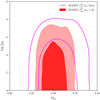 |
Fig. 5 Constraints obtained on log fR0 with eRASS1 clusters. No external cosmological datasets are combined with our data, which is shown in this figure. Constraints with a fixed neutrino mass are shown in red, while constraints for which the neutrino mass is free are shown in magenta. |
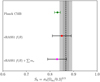 |
Fig. 6 Comparison of the S 8 parameter obtained using the different models. We show the 1σ uncertainties. The case introducing massless neutrinos is in red, while the one considering massive neutrinos is in pink. Results from the CMB are shown in green. The gray area represents the 68% and 95% confidence regions of the ΛCDM analysis from Ghirardini et al. (2024). |
5.3 Comparison with other constraints
Hereafter, all the constraints are shown at the 95% confidence level. In this work, we provide constraints on f (R) gravity with cluster abundance only for the first time. This allows us to test gravity with a self-consistent physical framework at a given physical scale and redshift range. Indeed, recent forecasts (Mitchell et al. 2021; Vogt et al. 2024) predict that future cluster abundance studies alone will be able to distinguish GR from alternative scenarios. Similarly, an alternative way of probing cosmology with the peaks of the matter density field is to consider WL peaks. Those also show promising results (Davies et al. 2024). This section compares our results with the ones obtained by other surveys and studies, from the smallest scales to the cosmological constraints. Indeed, due to the unknown nature of the potential modification of GR, it is important to test the theory at all physical scales.
Due to the nature of chameleon screening, the most stringent constraints are obtained from dwarf galaxies in cosmic voids. Desmond & Ferreira (2020) found |fR0| < –7.85 using galaxy morphology, which practically rules out the Hu-Sawicki model of f (R) gravity at astrophysical scales. Despite these results, testing the theory at larger scales is still relevant.
In the case of galaxy clusters, previous studies obtained consistent results with those presented in this work, but combining cluster abundances with the CMB and other LSS probes (Schmidt et al. 2009; Lombriser et al. 2012). When combined with CMB data, the most recent study by Cataneo et al. (2015) obtained log |fR0| < –4.79. We reach a similar precision with clusters only, primarily due to the statistical power of the eRASS1 cosmology sample, the largest ICM-selected sample to date.
Other probes at the cosmological scale typically obtain weaker constraints than the ones probing the small scales. They include the WL 2pt statistic. Tröster et al. (2021), using the KIDS 3 × 2 pt measurements of cosmic shear from KiDS-1000, did not find significant constraints on f (R) gravity using their data. Conversely, Liu et al. (2016) obtained log(fR0) < –5.15 combining measurements of the WL peaks with CMB priors. Hu et al. (2016) used supernovae data from JLA, WiggleZ, and CFHTLenS, in combination with CMB and BAO data, to find log(fR0) < –3.2. More recently, Kou et al. (2024) found an upper limit of log |fR0| < –4.61, cross-correlating CMB lensing with galaxy clustering.
Consequently, our results are consistent with the latest cosmological constraints. Astronomical probes on astrophysical and cosmological scales have found no evidence of a deviation from GR. Recent forecasts established for the Euclid survey (Casas et al. 2023) show that next-generation surveys will have the ability to distinguish GR from f (R) gravity with extreme precision, potentially ruling out the model definitively.
6 Discussion and conclusions
In this work, we present results on potential deviations from standard GR and ΛCDM using X-ray detected eRASS1 clusters, in combination with LS DR10-South for optical confirmation and redshift measurements, and DES, KiDS, and HSC for WL mass calibration. We have derived constraints on the HS model of f (R) gravity. We have considered both the case of massive and massless neutrinos.
All the models we have studied are statistically consistent with GR. Given the constraining power of eRASS1, we have chosen to present constraints from the cluster abundance only. This choice allows us to measure our parameters with a consistent physical framework for the first time. Indeed, this work shows that cluster counts alone have a great potential to constrain MG at the scale at which they are sensitive. Deeper surveys with eROSITA will significantly increase the constraints that we obtain here and might rival the results obtained at smaller scales. Overall, combined with the follow-up WL observations, the first eROSITA’s All-Sky survey has the statistical power to constrain the cosmological parameters with percent-level precision and to test the GR at large scales.
Lastly, we have investigated the consistency between our S8 measurements and the one given in the standard ΛCDM analysis and found good agreement. Modifying gravitation at the scale covered by cluster abundance does not significantly affect the S8 measurement. Our error bars are increased, but all posteriors are fully compatible. This emphasizes that the S 8 measurement provided in the ΛCDM analysis is robust against modifications and in good agreement with Planck Collaboration VI (2020).
Finally, the precision of our analysis mostly relies on the available HMF models. We have used the framework proposed by Hagstotz et al. (2019), while others like Cataneo et al. (2016) propose alternative approaches. Additional work will be necessary to increase the precision of our constraints by improving the reliability of the HMF, not only for f (R) gravity but also for any additional model of interest.
eROSITA, thus far, has collected data for more than four all-sky surveys. The final eRASS will detect about 105 galaxy clusters and groups (projected from the eFEDS results in Liu et al. 2022; Bulbul et al. 2022). The deeper eROSITA data and extensive cluster catalogs, in combination with state-of-the-art WL mass calibration, will allow us to tighten our constraints on the f (R) gravity models.
Acknowledgement
The full acknowledgments are available in Appendix B.
Appendix A Impact of the errors on the halo mass function
In this work, we use correcting factors for the HMF errors. Indeed, several methods yield different results for predicting the HMF in the HS- f (R) scenario. We use the prediction of Hagstotz et al. (2019), but alternative approaches exist like the one introduced by Cataneo et al. (2016). These different approaches yield up to 20% differences in the prediction of the HMF.
We use the analytic form introduced in Costanzi et al. (2019), where

We compare the posterior distribution of our parameters s and q and their impact on the HMF. This is shown in figure A.1. We fix the cosmology to the results of Planck Collaboration VI (2020). Then, we compute the HMF for GR (using the fit provided by Tinker et al. (2008)) and for different values of fR0. Assuming that the GR HMF is correct, we then use the posterior distribution of the parameters s and q to quantify their impact on the HMF. We show that including the slope and amplitude correction of the HMF corrects most of the expected difference between the different models of f (R), i.e., 20% difference. In the future, a more comprehensive modeling of the HMF uncertainties will be necessary to obtain high-precision measurements on the MG parameters.
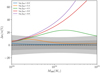 |
Fig. A.1 Relative difference of the HMF in different MG scenarios. ∆n = dn/dln M(fR0) – dn/d ln M, where dn/d ln M(fR0) is the HMF described with Eq. 20 and dn/d ln M is obtained with the GR fitting function from Tinker et al. (2008). We use the posterior distribution of the correcting parameters s and q and compare their impact to one of the MG parameters. The dark gray area corresponds to the 68% confidence level area, while the light gray one corresponds to the 95% confidence area. |
Appendix B Acknowledgements
The authors thank Prof. Catherine Heymans for her help and availability for the implementation of the blinding strategy and her helpful comments on the draft.
This work is based on data from eROSITA, the soft X-ray instrument aboard SRG, a joint Russian-German science mission supported by the Russian Space Agency (Roskosmos), in the interests of the Russian Academy of Sciences represented by its Space Research Institute (IKI), and the Deutsches Zentrum für Luft und Raumfahrt (DLR). The SRG spacecraft was built by the Lavochkin Association (NPOL) and its subcontractors and is operated by NPOL with support from the Max Planck Institute for Extraterrestrial Physics (MPE).
The development and construction of the eROSITA X-ray instrument was led by MPE, with contributions from the Dr. Karl Remeis Observatory Bamberg & ECAP (FAU Erlangen- Nuernberg), the University of Hamburg Observatory, the Leibniz Institute for Astrophysics Potsdam (AIP), and the Institute for Astronomy and Astrophysics of the University of Tübingen, with the support of DLR and the Max Planck Society. The Arge- lander Institute for Astronomy of the University of Bonn and the Ludwig Maximilians Universität Munich also participated in the science preparation for eROSITA.
The eROSITA data shown here were processed using the eSASS software system developed by the German eROSITA consortium (Brunner et al. 2022).
V. Ghirardini, E. Bulbul, A. Liu, C. Garrel, S. Zelmer, and X. Zhang acknowledge financial support from the European Research Council (ERC) Consolidator Grant under the European Union’s Horizon 2020 research and innovation program (grant agreement CoG DarkQuest No 101002585). CNES financially supported N. Clerc. M. Cataneo acknowledges the financial support provided by the Alexander von Humboldt Foundation through the Humboldt Research Fellowship program, as well as support from the Max Planck Society and the Alexander von Humboldt Foundation in the framework of the Max Planck-Humboldt Research Award endowed by the Federal Ministry of Education and Research. T. Schrabback and F. Kleinebreil acknowledge support from the German Federal Ministry for Economic Affairs and Energy (BMWi) provided through DLR under projects 50OR2002, 50OR2106, and 50OR2302, as well as the support provided by the Deutsche Forschungsgemeinschaft (DFG, German Research Foundation) under grant 415537506. The Innsbruck group also acknowledges support provided by the Austrian Research Promotion Agency (FFG) and the Federal Ministry of the Republic of Austria for Climate Action, Environment, Energy, Mobility, Innovation and Technology (BMK) via the Austrian Space Applications Programme with grant numbers 899537 and 900565.
The Legacy Surveys consist of three individual and complementary projects: the Dark Energy Camera Legacy Survey (DECaLS; Proposal ID #2014B-0404; PIs: David Schlegel and Arjun Dey), the Beijing-Arizona Sky Survey (BASS; NOAO Prop. ID #2015A-0801; PIs: Zhou Xu and Xiaohui Fan), and the Mayall z-band Legacy Survey (MzLS; Prop. ID #2016A-0453; PI: Arjun Dey). DECaLS, BASS, and MzLS together include data obtained, respectively, at the Blanco telescope, Cerro Tololo Inter-American Observatory, NSF’s NOIRLab; the Bok telescope, Steward Observatory, University of Arizona; and the Mayall telescope, Kitt Peak National Observatory, NOIRLab. Pipeline processing and analyses of the data were supported by NOIRLab and the Lawrence Berkeley National Laboratory (LBNL). The Legacy Surveys project is honored to be permitted to conduct astronomical research on Iolkam Du’ag (Kitt Peak), a mountain with particular significance to the Tohono O’odham Nation.
Funding for the DES Projects has been provided by the U.S. Department of Energy, the U.S. National Science Foundation, the Ministry of Science and Education of Spain, the Science and Technology FacilitiesCouncil of the United Kingdom, the Higher Education Funding Council for England, the National Center for Supercomputing Applications at the University of Illinois at Urbana-Champaign, the Kavli Institute of Cosmological Physics at the University of Chicago, the Center for Cosmology and Astro-Particle Physics at the Ohio State University, the Mitchell Institute for Fundamental Physics and Astronomy at Texas A&M University, Financiadora de Estudos e Proje- tos, Fundação Carlos Chagas Filho de Amparo à Pesquisa do Estado do Rio de Janeiro, Conselho Nacional de Desenvolvi- mento Científico e Tecnológico and the Ministério da Ciência, Tecnologia e Inovação, the Deutsche Forschungsgemeinschaft, and the Collaborating Institutions in the Dark Energy Survey.
The Collaborating Institutions are Argonne National Laboratory, the University of California at Santa Cruz, the University of Cambridge, Centro de Investigaciones Energéticas, Medioambientales y Tecnológicas-Madrid, the University of Chicago, University College London, the DES-Brazil Consortium, the University of Edinburgh, the Eidgenössische Technische Hochschule (ETH) Zürich, Fermi National Accelerator Laboratory, the University of Illinois at Urbana-Champaign, the Institut de Ciències de l’Espai (IEEC/CSIC), the Institut de Física d’Altes Energies, Lawrence Berkeley National Laboratory, the Ludwig-Maximilians Universität München and the associated Excellence Cluster Universe, the University of Michigan, the National Optical Astronomy Observatory, the University of Nottingham, The Ohio State University, the OzDES Membership Consortium, the University of Pennsylvania, the University of Portsmouth, SLAC National Accelerator Laboratory, Stanford University, the University of Sussex, and Texas A&M University.
Based on observations made with ESO Telescopes at the La Silla Paranal Observatory under program IDs 177.A-3016, 177.A-3017, 177.A-3018, and 179.A-2004, and on data products produced by the KiDS consortium. The KiDS production team acknowledges support from Deutsche Forschungsgemeinschaft, ERC, NOVA, and NWO-M grants; Target; the University of Padova; and the University Federico II (Naples).
This paper makes use of software developed for the Large Synoptic Survey Telescope. We thank the LSST Project for making their code available as free software at http://dm.lsst.org
This work made use of the following Python software packages: SciPy1 (Virtanen et al. 2020), Matplotlib2 (Hunter 2007), Astropy3 (Astropy Collaboration 2022), NumPy4 (Harris et al. 2020), CAMB (Lewis & Challinor 2011), pyCCL5 (Chisari et al. 2019), GPy6 (GPy 2012), climin7 (Bayer et al. 2015), ultranest8 (Buchner 2021)
References
- Aihara, H., Armstrong, R., Bickerton, S., et al. 2018, PASJ, 70, S8 [NASA ADS] [Google Scholar]
- Alam, S., Ata, M., Bailey, S., et al. 2017, MNRAS, 470, 2617 [Google Scholar]
- Amon, A., Gruen, D., Troxel, M. A., et al. 2022, Phys. Rev. D, 105, 023514 [NASA ADS] [CrossRef] [Google Scholar]
- Artis, E., Melin, J.-B., Bartlett, J. G., & Murray, C. 2021, A&A, 649, A47 [NASA ADS] [CrossRef] [EDP Sciences] [Google Scholar]
- Asgari, M., Lin, C.-A., Joachimi, B., et al. 2021, A&A, 645, A104 [NASA ADS] [CrossRef] [EDP Sciences] [Google Scholar]
- Astropy Collaboration (Price-Whelan, A. M., et al.) 2022, ApJ, 935, 167 [NASA ADS] [CrossRef] [Google Scholar]
- Bartelmann, M., & Schneider, P. 2001, Phys. Rep., 340, 291 [Google Scholar]
- Bayer, J., Osendorfer, C., Diot-Girard, S., Rueckstiess, T., & Urban, S. 2015, TUM, Tech. Rep. [Google Scholar]
- Bekenstein, J. D., & Sanders, R. H. 1994, ApJ, 429, 480 [NASA ADS] [CrossRef] [Google Scholar]
- Bennett, C. L., Larson, D., Weiland, J. L., et al. 2013, ApJS, 208, 20 [Google Scholar]
- Bocquet, S., Saro, A., Mohr, J. J., et al. 2015, ApJ, 799, 214 [NASA ADS] [CrossRef] [Google Scholar]
- Bocquet, S., Dietrich, J. P., Schrabback, T., et al. 2019, ApJ, 878, 55 [Google Scholar]
- Bocquet, S., Heitmann, K., Habib, S., et al. 2020, ApJ, 901, 5 [Google Scholar]
- Bocquet, S., Grandis, S., Bleem, L. E., et al. 2024a, Phys. Rev. D, submitted [arXiv:2310.12213v2] [Google Scholar]
- Bocquet, S., Grandis, S., Bleem, L. E., et al. 2024b, Phys. Rev. D, submitted [arXiv:2401.02075] [Google Scholar]
- Brunner, H., Liu, T., Lamer, G., et al. 2022, A&A, 661, A1 [NASA ADS] [CrossRef] [EDP Sciences] [Google Scholar]
- Buchner, J. 2021, The Journal of Open Source Software, 6, 3001 [NASA ADS] [CrossRef] [Google Scholar]
- Bulbul, E., Liu, A., Pasini, T., et al. 2022, A&A, 661, A10 [NASA ADS] [CrossRef] [EDP Sciences] [Google Scholar]
- Bulbul, E., Liu, A., Kluge, M., et al. 2024, A&A, 685, A106 [NASA ADS] [CrossRef] [EDP Sciences] [Google Scholar]
- Casas, S., Cardone, V. F., Sapone, D., et al. 2023, A&A, submitted [arXiv:2306.11053] [Google Scholar]
- Cataneo, M., Rapetti, D., Schmidt, F., et al. 2015, Phys. Rev. D, 92, 044009 [NASA ADS] [CrossRef] [Google Scholar]
- Cataneo, M., Rapetti, D., Lombriser, L., & Li, B. 2016, J. Cosmology Astropart. Phys., 2016, 024 [CrossRef] [Google Scholar]
- Chisari, N. E., Alonso, D., Krause, E., et al. 2019, CCL: Core Cosmology Library, Astrophysics Source Code Library [record ascl:1901.003] [Google Scholar]
- Clerc, N., & Finoguenov, A. 2023, in Handbook of X-ray and Gamma-ray Astrophysics, eds. C. Bambi, & A. Santangelo, 123 [Google Scholar]
- Clerc, N., Comparat, J., Seppi, R., et al. 2024, A&A, 687, A238 [NASA ADS] [CrossRef] [EDP Sciences] [Google Scholar]
- Costanzi, M., Villaescusa-Navarro, F., Viel, M., et al. 2013, J. Cosmology Astropart. Phys., 2013, 012 [CrossRef] [Google Scholar]
- Costanzi, M., Rozo, E., Simet, M., et al. 2019, MNRAS, 488, 4779 [NASA ADS] [CrossRef] [Google Scholar]
- Davies, C. T., Harnois-Déraps, J., Li, B., et al. 2024, MNRAS, 533, 3546 [NASA ADS] [CrossRef] [Google Scholar]
- De Felice, A., & Tsujikawa, S. 2010, Liv. Rev. Relativ., 13, 3 [NASA ADS] [CrossRef] [Google Scholar]
- Desmond, H., & Ferreira, P. G. 2020, Phys. Rev. D, 102, 104060 [NASA ADS] [CrossRef] [Google Scholar]
- Despali, G., Giocoli, C., Angulo, R. E., et al. 2016, MNRAS, 456, 2486 [NASA ADS] [CrossRef] [Google Scholar]
- Duffy, A. R., Schaye, J., Kay, S. T., & Dalla Vecchia, C. 2008, MNRAS, 390, L64 [Google Scholar]
- Eisenstein, D. J., Zehavi, I., Hogg, D. W., et al. 2005, ApJ, 633, 560 [Google Scholar]
- Euclid Collaboration (Castro, T., et al.) 2023, A&A, 671, A100 [CrossRef] [EDP Sciences] [Google Scholar]
- Euclid Collaboration (Giocoli, C., et al.) 2024, A&A, 681, A67 [NASA ADS] [CrossRef] [EDP Sciences] [Google Scholar]
- Freedman, W. L., Madore, B. F., Hatt, D., et al. 2019, ApJ, 882, 34 [Google Scholar]
- Fumagalli, A., Costanzi, M., Saro, A., Castro, T., & Borgani, S. 2024, A&A, 682, A148 [NASA ADS] [CrossRef] [EDP Sciences] [Google Scholar]
- Gannouji, R., Moraes, B., & Polarski, D. 2009, J. Cosmology Astropart. Phys., 2009, 034 [CrossRef] [Google Scholar]
- Garrel, C., Pierre, M., Valageas, P., et al. 2022, A&A, 663, A3 [NASA ADS] [CrossRef] [EDP Sciences] [Google Scholar]
- Gatti, M., Sheldon, E., Amon, A., et al. 2021, MNRAS, 504, 4312 [NASA ADS] [CrossRef] [Google Scholar]
- Ghirardini, V., Bulbul, E., Artis, E., et al. 2024, A&A, 689, A298 [NASA ADS] [CrossRef] [EDP Sciences] [Google Scholar]
- Giblin, B., Heymans, C., Asgari, M., et al. 2021, A&A, 645, A105 [NASA ADS] [CrossRef] [EDP Sciences] [Google Scholar]
- Giocoli, C., Baldi, M., & Moscardini, L. 2018, MNRAS, 481, 2813 [Google Scholar]
- GPy 2012, GPy: A Gaussian process framework in python, http://github.com/SheffieldML/GPy [Google Scholar]
- Grandis, S., Bocquet, S., Mohr, J. J., Klein, M., & Dolag, K. 2021a, MNRAS, 507, 5671 [NASA ADS] [CrossRef] [Google Scholar]
- Grandis, S., Mohr, J. J., Costanzi, M., et al. 2021b, MNRAS, 504, 1253 [NASA ADS] [CrossRef] [Google Scholar]
- Grandis, S., Ghirardini, V., Bocquet, S., et al. 2024, A&A, 687, A178 [NASA ADS] [CrossRef] [EDP Sciences] [Google Scholar]
- Gupta, S., Hellwing, W. A., Bilicki, M., & García-Farieta, J. E. 2022, Phys. Rev. D, 105, 043538 [NASA ADS] [CrossRef] [Google Scholar]
- Hagstotz, S., Costanzi, M., Baldi, M., & Weller, J. 2019, MNRAS, 486, 3927 [Google Scholar]
- Harris, C. R., Millman, K. J., van der Walt, S. J., et al. 2020, Nature, 585, 357 [NASA ADS] [CrossRef] [Google Scholar]
- Hildebrandt, H., van den Busch, J. L., Wright, A. H., et al. 2021, A&A, 647, A124 [EDP Sciences] [Google Scholar]
- Hu, W., & Kravtsov, A. V. 2003, ApJ, 584, 702 [Google Scholar]
- Hu, W., & Sawicki, I. 2007, Phys. Rev. D, 76, 064004 [CrossRef] [Google Scholar]
- Hu, B., Raveri, M., Frusciante, N., & Silvestri, A. 2014, Phys. Rev. D, 89, 103530 [Google Scholar]
- Hu, B., Raveri, M., Rizzato, M., & Silvestri, A. 2016, MNRAS, 459, 3880 [Google Scholar]
- Huff, E., & Mandelbaum, R. 2017, arXiv e-prints [arXiv:1702.02600] [Google Scholar]
- Hunter, J. D. 2007, Comput. Sci. Eng., 9, 90 [NASA ADS] [CrossRef] [Google Scholar]
- Ider Chitham, J., Comparat, J., Finoguenov, A., et al. 2020, MNRAS, 499, 4768 [NASA ADS] [CrossRef] [Google Scholar]
- Khoury, J., & Weltman, A. 2004, Phys. Rev. D, 69, 044026 [CrossRef] [Google Scholar]
- Kluge, M., Comparat, J., Liu, A., et al. 2024, A&A, 688, A210 [NASA ADS] [CrossRef] [EDP Sciences] [Google Scholar]
- Knebe, A., Pearce, F. R., Lux, H., et al. 2013, MNRAS, 435, 1618 [NASA ADS] [CrossRef] [Google Scholar]
- Kopp, M., Appleby, S. A., Achitouv, I., & Weller, J. 2013, Phys. Rev. D, 88, 084015 [NASA ADS] [CrossRef] [Google Scholar]
- Kou, R., Murray, C., & Bartlett, J. G. 2024, A&A, 686, A193 [NASA ADS] [CrossRef] [EDP Sciences] [Google Scholar]
- Kuijken, K., Heymans, C., Dvornik, A., et al. 2019, A&A, 625, A2 [NASA ADS] [CrossRef] [EDP Sciences] [Google Scholar]
- Lacasa, F., & Grain, J. 2019, A&A, 624, A61 [NASA ADS] [CrossRef] [EDP Sciences] [Google Scholar]
- Lesci, G. F., Nanni, L., Marulli, F., et al. 2022, A&A, 665, A100 [NASA ADS] [CrossRef] [EDP Sciences] [Google Scholar]
- Lesgourgues, J. 2011, arXiv e-prints [arXiv:1104.2932] [Google Scholar]
- Lewis, A., & Challinor, A. 2011, CAMB: Code for Anisotropies in the Microwave Background, Astrophysics Source Code Library [record ascl:1102.026] [Google Scholar]
- Li, B., Zhao, G.-B., & Koyama, K. 2012, MNRAS, 421, 3481 [NASA ADS] [CrossRef] [Google Scholar]
- Li, X., Miyatake, H., Luo, W., et al. 2022, PASJ, 74, 421 [NASA ADS] [CrossRef] [Google Scholar]
- Li, X., Zhang, T., Sugiyama, S., et al. 2023, Phys. Rev. D, 108, 123518 [CrossRef] [Google Scholar]
- Liu, X., Li, B., Zhao, G.-B., et al. 2016, Phys. Rev. Lett., 117, 051101 [NASA ADS] [CrossRef] [Google Scholar]
- Liu, A., Bulbul, E., Ghirardini, V., et al. 2022, A&A, 661, A2 [NASA ADS] [CrossRef] [EDP Sciences] [Google Scholar]
- Lombriser, L., Slosar, A., Seljak, U., & Hu, W. 2012, Phys. Rev. D, 85, 124038 [NASA ADS] [CrossRef] [Google Scholar]
- Lombriser, L., Li, B., Koyama, K., & Zhao, G.-B. 2013, Phys. Rev. D, 87, 123511 [NASA ADS] [CrossRef] [Google Scholar]
- Mantz, A. B., von der Linden, A., Allen, S. W., et al. 2015, MNRAS, 446, 2205 [Google Scholar]
- Merloni, A., Lamer, G., Liu, T., et al. 2024, A&A, 682, A34 [NASA ADS] [CrossRef] [EDP Sciences] [Google Scholar]
- Mitchell, M. A., He, J.-h., Arnold, C., & Li, B. 2018, MNRAS, 477, 1133 [NASA ADS] [CrossRef] [Google Scholar]
- Mitchell, M. A., Arnold, C., & Li, B. 2021, MNRAS, 508, 4157 [NASA ADS] [CrossRef] [Google Scholar]
- Nakamura, T. T., & Suto, Y. 1997, Progr. Theor. Phys., 97, 49 [NASA ADS] [CrossRef] [Google Scholar]
- Navarro, J. F., Frenk, C. S., & White, S. D. M. 1996, ApJ, 462, 563 [Google Scholar]
- Oyaizu, H. 2008, Phys. Rev. D, 78, 123523 [NASA ADS] [CrossRef] [Google Scholar]
- Percival, W. J., & White, M. 2009, MNRAS, 393, 297 [NASA ADS] [CrossRef] [Google Scholar]
- Perlmutter, S., Aldering, G., Goldhaber, G., et al. 1999, ApJ, 517, 565 [Google Scholar]
- Planck Collaboration VI. 2020, A&A, 641, A6 [NASA ADS] [CrossRef] [EDP Sciences] [Google Scholar]
- Predehl, P., Andritschke, R., Arefiev, V., et al. 2021, A&A, 647, A1 [EDP Sciences] [Google Scholar]
- Preston, C., Amon, A., & Efstathiou, G. 2023, MNRAS, 525, 5554 [NASA ADS] [CrossRef] [Google Scholar]
- Riess, A. G., Filippenko, A. V., Challis, P., et al. 1998, AJ, 116, 1009 [Google Scholar]
- Riess, A. G., Casertano, S., Yuan, W., Macri, L. M., & Scolnic, D. 2019, ApJ, 876, 85 [Google Scholar]
- Ruan, C.-Z., Cuesta-Lazaro, C., Eggemeier, A., et al. 2023, MNRAS, 527, 2490 [NASA ADS] [CrossRef] [Google Scholar]
- Salvati, L., Douspis, M., & Aghanim, N. 2020, A&A, 643, A20 [NASA ADS] [CrossRef] [EDP Sciences] [Google Scholar]
- Sanders, J. S., Fabian, A. C., Russell, H. R., & Walker, S. A. 2018, MNRAS, 474, 1065 [NASA ADS] [CrossRef] [Google Scholar]
- Schmidt, F. 2010, Phys. Rev. D, 81, 103002 [NASA ADS] [CrossRef] [Google Scholar]
- Schmidt, F., Vikhlinin, A., & Hu, W. 2009, Phys. Rev. D, 80, 083505 [NASA ADS] [CrossRef] [Google Scholar]
- Seppi, R., Comparat, J., Ghirardini, V., et al. 2024, A&A, 686, A196 [NASA ADS] [CrossRef] [EDP Sciences] [Google Scholar]
- Sheldon, E. S., & Huff, E. M. 2017, ApJ, 841, 24 [NASA ADS] [CrossRef] [Google Scholar]
- Sheth, R. K., & Tormen, G. 2002, MNRAS, 329, 61 [Google Scholar]
- Sunayama, T., Miyatake, H., Sugiyama, S., et al. 2023, arXiv e-prints [arXiv:2309.13025] [Google Scholar]
- Tinker, J., Kravtsov, A. V., Klypin, A., et al. 2008, ApJ, 688, 709 [Google Scholar]
- Tröster, T., Asgari, M., Blake, C., et al. 2021, A&A, 649, A88 [NASA ADS] [CrossRef] [EDP Sciences] [Google Scholar]
- Troxel, M. A., MacCrann, N., Zuntz, J., et al. 2018, Phys. Rev. D, 98, 043528 [Google Scholar]
- Tsujikawa, S., Gannouji, R., Moraes, B., & Polarski, D. 2009, Phys. Rev. D, 80, 084044 [NASA ADS] [CrossRef] [Google Scholar]
- Vikhlinin, A., Burenin, R. A., Ebeling, H., et al. 2009, ApJ, 692, 1033 [Google Scholar]
- Virtanen, P., Gommers, R., Oliphant, T. E., et al. 2020, Nature Methods, 17, 261 [CrossRef] [Google Scholar]
- Vogt, S. M. L., Bocquet, S., Davies, C. T., Mohr, J. J., & Schmidt, F. 2024, Phys. Rev. D, 109, 123503 [NASA ADS] [CrossRef] [Google Scholar]
- von Braun-Bates, F., Winther, H. A., Alonso, D., & Devriendt, J. 2017, J. Cosmology Astropart. Phys., 2017, 012 [CrossRef] [Google Scholar]
- Wang, Z., Mirpoorian, S. H., Pogosian, L., Silvestri, A., & Zhao, G.-B. 2023, J. Cosmology Astropart. Phys., 2023, 038 [CrossRef] [Google Scholar]
- Wolf, W. J., & Ferreira, P. G. 2023, Phys. Rev. D, 108, 103519 [NASA ADS] [CrossRef] [Google Scholar]
- Wright, C. O., & Brainerd, T. G. 2000, ApJ, 534, 34 [Google Scholar]
- Wright, A. H., Hildebrandt, H., van den Busch, J. L., & Heymans, C. 2020, A&A, 637, A100 [NASA ADS] [CrossRef] [EDP Sciences] [Google Scholar]
- Xu, L. 2015, arXiv e-prints [arXiv: 1506.03232] [Google Scholar]
- Zhao, G.-B., Li, B., & Koyama, K. 2011, Phys. Rev. D, 83, 044007 [NASA ADS] [CrossRef] [Google Scholar]
- Zubeldia, Í., & Challinor, A. 2019, MNRAS, 489, 401 [NASA ADS] [CrossRef] [Google Scholar]
- Zucca, A., Pogosian, L., Silvestri, A., & Zhao, G. B. 2019, J. Cosmology Astropart. Phys., 2019, 001 [CrossRef] [Google Scholar]
- Zumalacárregui, M., Bellini, E., Sawicki, I., Lesgourgues, J., & Ferreira, P. G. 2017, J. Cosmology Astropart. Phys., 2017, 019 [CrossRef] [Google Scholar]
All Tables
Priors on the cosmological parameters used in this analysis when they are involved in the corresponding model.
All Figures
|
Fig. 1 Estimation of the scale and redshift sensitivity of the different cosmological probes, adapted from Preston et al. (2023). The background colors, from blue to green, represent the transition from the linear to the nonlinear regime. We represent cluster abundance with the red rectangle. The cosmology sample of eRASS1 spans the redshift range 0.1 < z < 0.8, as is represented by the solid red rectangle. Future data releases and experiments will increase the upper limit of this interval to the hatched red rectangle. Cluster abundance experiments thus probe a specific regime at LSSs and the nearby Universe, offering a complementary window on structure formation. The constraints from cluster clustering (Seppi et al. 2024) are omitted here. Additionally, the X-ray power spectrum might probe smaller scales. |
| In the text | |
|
Fig. 2 Relative difference (in percentages) of the HMF at z = 0.5 when we increase fR0. We note that ∆n = dn/d ln M(fR0) – dn/d ln M, where dn/d ln M(fR0) is the HMF described with Eq. (20) and dn/d ln M is obtained with the GR fitting function from Tinker et al. (2008). Increased values of fR0 create more massive halos. |
| In the text | |
|
Fig. 3 Comparison of the posteriors on the scaling relation obtained in the f (R) framework (the mass of the neutrinos is fixed) and the standard ΛCDM analysis presented in Ghirardini et al. (2024) (gray). The different models are fully consistent with one another. We overplot the contours obtained from WL only from Grandis et al. (2024) (green). |
| In the text | |
|
Fig. 4 Comparison of the posteriors obtained on the Ω – σ8 plane. We represent the ΛCDM analysis introduced in Ghirardini et al. (2024) in gray, while the posteriors of HS- f (R) case are shown in red. |
| In the text | |
|
Fig. 5 Constraints obtained on log fR0 with eRASS1 clusters. No external cosmological datasets are combined with our data, which is shown in this figure. Constraints with a fixed neutrino mass are shown in red, while constraints for which the neutrino mass is free are shown in magenta. |
| In the text | |
|
Fig. 6 Comparison of the S 8 parameter obtained using the different models. We show the 1σ uncertainties. The case introducing massless neutrinos is in red, while the one considering massive neutrinos is in pink. Results from the CMB are shown in green. The gray area represents the 68% and 95% confidence regions of the ΛCDM analysis from Ghirardini et al. (2024). |
| In the text | |
|
Fig. A.1 Relative difference of the HMF in different MG scenarios. ∆n = dn/dln M(fR0) – dn/d ln M, where dn/d ln M(fR0) is the HMF described with Eq. 20 and dn/d ln M is obtained with the GR fitting function from Tinker et al. (2008). We use the posterior distribution of the correcting parameters s and q and compare their impact to one of the MG parameters. The dark gray area corresponds to the 68% confidence level area, while the light gray one corresponds to the 95% confidence area. |
| In the text | |
Current usage metrics show cumulative count of Article Views (full-text article views including HTML views, PDF and ePub downloads, according to the available data) and Abstracts Views on Vision4Press platform.
Data correspond to usage on the plateform after 2015. The current usage metrics is available 48-96 hours after online publication and is updated daily on week days.
Initial download of the metrics may take a while.