| Issue |
A&A
Volume 687, July 2024
|
|
|---|---|---|
| Article Number | A231 | |
| Number of page(s) | 9 | |
| Section | The Sun and the Heliosphere | |
| DOI | https://doi.org/10.1051/0004-6361/202449551 | |
| Published online | 16 July 2024 | |
High-precision spectral inversions: Determining what is important for the accurate definition of incident radiation boundary conditions
1
Astronomical Institute, The Czech Academy of Sciences, 251 65 Ondřejov, Czech Republic
e-mail: gunar@asu.cas.cz
2
Center of Excellence ‘Solar and Stellar Activity’, University of Wroclaw, Wroclaw, Poland
Received:
8
February
2024
Accepted:
28
April
2024
Context. Spectral inversions are used to analyse spectroscopic observations with the aim of deriving the physical properties of the observed plasma, such as the kinetic temperature, density, pressure, degree of ionisation, or macroscopic velocities. One of the key factors ensuring the high precision of the derived plasma properties is having accurately defined input parameters of the models on which spectral inversions rely. The illumination, which chromospheric and coronal structures receive from the solar surface (and corona), is one of the most crucial input parameters of these models.
Aims. We do not perform spectral inversions in this work. Our aim is to study two important factors that contribute to the accurate definition of the incident radiation boundary conditions: the altitude above the solar surface and the dynamics of the illuminated plasma. This investigation takes into account a diverse range of solar structures from the high-rising eruptive prominences to low-lying spicules.
Methods. To study the influence of the altitude and dynamics of the observed plasma on the incident radiation boundary conditions, we used geometrical principles valid for any spectral line. However, to demonstrate the strong impact of dynamics, we considered the specific case of narrow spectral lines of Mg II H&K, which are highly sensitive to the presence of velocities.
Results. We argue that the altitude of the illuminated plasma strongly influences the way we need to define the incident radiation boundary conditions to achieve the most accurate results. For low-lying structures, generally below 50 000 km, the incident radiation may need to be specified directly from the composition of the portion of the solar disc that illuminates them. For high-altitude structures, generally above 300 000 km, the fraction of the solar disc illuminating the analysed plasma is large enough to be realistically approximated by the composition of the entire disc. We also show that for the narrow spectral lines, such as the Mg II H&K lines, the impact of dynamics on the incident radiation intensity and profile shapes starts from radial velocities of 30 km s−1. Such velocities are even exhibited by the fine structures of quiescent prominences and are easily exceeded in spicules or eruptive prominences.
Conclusions. The two aspects of the incident radiation definition studied here are relevant for spectral inversions based on any kind of modelling approach. However, their impact on the precision of the results of spectral inversions is likely less significant than the impact of the choice of the complexity of the model geometry, for example.
Key words: radiative transfer / techniques: spectroscopic / Sun: atmosphere / Sun: filaments / prominences / Sun: UV radiation
© The Authors 2024
 Open Access article, published by EDP Sciences, under the terms of the Creative Commons Attribution License (https://creativecommons.org/licenses/by/4.0), which permits unrestricted use, distribution, and reproduction in any medium, provided the original work is properly cited.
This article is published in open access under the Subscribe to Open model. Subscribe to A&A to support open access publication.
1. Introduction
Spectral inversions are a class of inversion techniques used for the analysis of spectroscopic observations. These techniques rely on as-realistic-as-possible models of the plasma properties of the studied solar features. They then use sophisticated radiative transfer simulations to produce synthetic spectra emerging from the modelled plasma. Next, the synthetic spectral-line profiles are compared with the observed spectra to search for a close match of intensities and profile shapes. When a match between the observed and the synthetic spectra is found, the particular plasma properties of the model are deemed to be the same as those of the observed plasma. In this way, we can obtain information about the physical properties of the observed plasma, such as kinetic temperature, density, pressure, degree of ionisation, or macroscopic velocities. With regard to these goals, spectral inversions are related to, but distinct from, the spectro-polarimetric inversions used to derive information about the topology and strength of the solar magnetic fields (see e.g. the review by López Ariste 2015).
In recent years, increasingly more sophisticated spectral inversions have been used in studies of chromosphere, and chromospheric or coronal structures. For example, Vial et al. (2019) and Ruan et al. (2019) analysed spectral observations of quiescent solar prominences, Koza et al. (2019) performed a spectral analysis of a loop prominence, and the properties of the chromosphere were investigated by Sainz Dalda et al. (2019) and da Silva Santos et al. (2020). Spectral observations of an eruptive prominence were analysed by Zhang et al. (2019). The kinetic temperature and plasma density in quiescent prominences were derived from spectroscopic observations by Barczynski et al. (2021), Peat et al. (2021, 2023), and Jejčič et al. (2022), or by Heinzel et al. (2022). With the increasingly better capabilities and precision of spectral inversions, it is becoming clear that the input parameters of the models on which these techniques are based will also need to be defined with a very high level of accuracy.
For cool chromospheric and coronal structures, one of the most crucial input parameters is incident radiation. This represents the dominant outer source of energy for plasma located above the solar surface. What makes the incident radiation boundary condition critically important for spectral inversions is the sensitivity of the spectra emerging from the structures to the changes in the illumination. Often, an increase (or decrease) in the intensity of the incident radiation can result in nearly the same change in the spectra emerging from the observed structures as a result of scattering processes. This was demonstrated by Gunár et al. (2020, 2022) using the hydrogen Lyman lines and Mg II H&K lines. Such sensitivity to the incident radiation means that models with otherwise identical plasma parameters (temperature, pressure, etc.) will produce different synthetic spectra if different incident radiation is assumed. If we simplify the results of Gunár et al. (2020, 2022), we can say that when the incident radiation is changed by 10, 20, or 30%, the resulting synthetic profiles (in this case the Lyman and Mg II H&K lines) are also likely to change by 10, 20, or 30%. However, this has strong implications for the accuracy of the results of spectral inversions. Why? Because when using the spectral inversion techniques, we rely on a realistic representation of the physical mechanisms governing the studied solar structures, but we do not a priori know the values of the plasma parameters (such as temperature or pressure). On the contrary, we aim to derive these properties of the observed plasma from the observed spectra. Consequently, inversions of two sets of observed spectra with different characteristics will result in different derived values of the plasma parameters when we use identical boundary conditions. Clearly, this is in conflict with the situation where the difference in the spectra is caused not by different plasma properties, but by different incident radiation. This is especially true when we realise that the change in the incident radiation intensity between the minimum and maximum of the solar cycle can reach even up to 100% (see e.g. Gunár et al. 2020; Koza et al. 2022). This then clearly demonstrates that properly defined incident radiation boundary conditions are key for high-precision spectral inversions.
In the current paper, we focus on two aspects of the incident radiation important for its accurate definition: altitude and the dynamics of the illuminated plasma. The altitude (Sect. 2) plays a dual role in the definition of the incident radiation boundary conditions. The first is the geometrical dilution of the intensity – the higher above the solar surface the plasma is located, the smaller the spatial angle from which it receives illumination, and the less intensity it receives. This dilution factor is an integral part of all radiative transfer models and is well described in Jejčič & Heinzel (2009) and Labrosse (2015), for example. The second, less trivial role of altitude is the way in which it determines the area of the solar surface from which the plasma receives the illumination. Put simply, the height of the analysed structure above the solar surface determines the part of the surface that the structure ‘sees’. As we show in Sect. 2, the visible solar surface may represent only a small fraction of the entire solar hemisphere. In itself, this would not matter if the Sun did not vary in time. Or, if its variation would be homogeneous over the entire solar surface. However, this is not the case. Active regions, sunspots, coronal holes, filaments, and other manifestations of solar activity are distributed highly inhomogeneously over the solar surface. Therefore, the extent of the visible portion of the solar surface serves as a strong modulator, determining the amplitude of change in the incident radiation. The altitude also influences the shape of the centre-to-limb variation of the solar-disc radiation that the plasma ‘sees’. We address this issue in Sect. 3.
The dynamics of the illuminated plasma (Sect. 4) influence the incident radiation due to the Doppler shift. However, this effect is more complex than a simple shift of a spectral profile in wavelengths. Known as Doppler dimming or brightening (see e.g. Heinzel & Rompolt 1987), the effect depends on the shape of the illuminating spectral line. In general, if the illumination comes in the form of an absorption spectral line, the radially moving plasma will receive higher intensity radiation than the static plasma, resulting in an overall brightening of the observed structures. In contrast, if the incident radiation comes in the form of an emission line, the Doppler shift will cause the radially moving plasma to receive less radiation, resulting in a dimming of the observed structures. However, the situation in specific cases is not as straightforward as this simple description suggests. As we show in Sect. 4, the high-precision definition of the incident radiation depends on the combination of the actual velocity vector, the altitude, the presence of the centre-to-limb variation in the illumination from the solar surface, and the shape of the illuminating spectral line profile. Here, the distinction is not only between the absorption and emission lines, but also between broad spectral lines that are not too sensitive to the velocity effects (such as Lyman lines) and narrow spectral lines that are strongly affected by the presence of velocities. In the present paper, we focus on the velocity-sensitive spectral lines, such as Mg II H&K or Ca II H&K. The broad spectral lines of hydrogen (Lyman-α, Lyman-β and Hα) were studied by, for example, Gontikakis et al. (1997b) or Heinzel et al. (2016). The broad He I lines were studied by, for example, Labrosse et al. (2007).
2. Altitude above the solar surface
From a simple look at the geometry of the situation of a structure located near a spherical surface (Fig. 1), it is clear that such a structure does not receive illumination from the entire hemisphere. The portion of the surface that is visible to the structure depends on the distance from the surface, that is, its altitude. There is nothing surprising about this. One may thus question why this aspect is relevant for a high-fidelity definition of the incident radiation boundary conditions. This is because of the highly localised variability of the solar-disc radiation during the solar cycle. Active regions, plages, coronal holes, and filaments do not cover the entire solar disc, nor are they distributed homogeneously. Therefore, their presence (or absence) within the visible portion of the solar disc from the given altitude will strongly influence the properties of the incident radiation received by the illuminated structures.
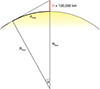 |
Fig. 1. Geometry of situation in which a structure located at an altitude of 100 000 km receives illumination from the solar surface. The arc length of dmax corresponds to the maximum visible distance from the given altitude. |
To quantify the influence of the altitude on the definition of the incident radiation boundary conditions, we focused on altitudes above the photosphere ranging from 2000 km to 5RSun. For each altitude (H), we derived the polar angle θ corresponding to the maximum extent of the solar surface visible from a given altitude (see Fig. 1). The values of θ, derived from the equation
are listed in Table 1 for all considered altitudes. Here, RSun is the nominal solar radius of 695 700 km.
Influence of altitude on the visible area of the solar disc.
To better visualise the extent of the area visible from a given altitude, we used the maximum visible distance (dmax) expressed as the arc length corresponding to the angle θ. This maximum arc length is derived as
We also calculated the percentage of the area of the solar hemisphere visible from a given altitude. The visible surface area is derived as the area of a spherical cup, given by the equation

Both the maximum visible distance and the percentage of the solar hemisphere visible from a given altitude are listed in Table 1.
From Table 1, it is clear that the total visible area from low-lying structures is very restricted. For example, from an altitude of 10 000 km, the visible area of the solar surface corresponds to just 1.42% of the area of the solar hemisphere. The portion of the Sun from which structures in the corona receive illumination increases to 12.57% at an altitude of 100 000 km and 50% at an altitude of 1RSun.
Because it may be difficult to imagine the extent of the visible surface from a given altitude in the spherical projection, we show several scenarios in Fig. 2. This figure shows the extent of the surface illuminating plasma at a given altitude for the range of typical altitudes of quiescent prominences. We place the hypothetical illuminated structure at different locations on the solar disc, ranging from the disc centre to the limb.
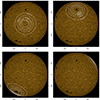 |
Fig. 2. Illustration of extent of solar surface from which structures at altitudes of 10 000 km, 20 000 km, 30 000 km, 50 000 km, and 100 000 km receive illumination. The background image is a full-Sun mosaic obtained on 2019 October 20 in the Mg II K line centre by the Interface Region Imaging Spectrograph (IRIS; De Pontieu et al. 2014). |
3. Centre-to-limb variation at different altitudes
In many spectral lines used for the diagnostics of solar plasmas (such as the Mg II H&K lines and the Ca II H&K lines), the illumination from the solar disc is affected by a systematic variation of the intensity and shape of the spectral profiles depending on the distance from the disc centre. This centre-to-limb variation is derived using the observations from the distance of 1 AU (see e.g. Gunár et al. 2021 or Pietrow et al. 2023). The centre-to-limb variation is typically described as a function of μ: the cosine of the angle between the incident ray from a given position on the disc and the local radial direction (angle γ in Fig. 3). The values of μ thus vary from μ = 1 at the disc centre to μ = 0 at the limb.
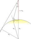 |
Fig. 3. Geometry of situation in which a structure located at an altitude of RSun receives illuminations from the solar surface. |
At this point, it is important to realise that the centre-to-limb variation we see from the distance of 1 AU does not disappear when we come closer to the solar surface. Even at very low altitudes, there are always rays (lines of sight) that are tangential to the solar surface (μ = 0), as well as those that are perpendicular to it (μ = 1). However, the distribution of μ values over the visible solar surface slightly varies with the altitude.
To show this variation, we divide the angle α in half and derive the μ values for the angle α/2 at different altitudes. In Fig. 3, we illustrate the geometry of the problem we solve to find the μ (cos γ) values corresponding to the angle α/2. To derive the angle γ for a given altitude H, we need to find values of the unknowns a and x by solving the following set of equations:
Computing μ corresponding to the angle α/2 allows us to assess how much the μ function at a given altitude differs from that observed from 1 AU. The results summarised in Table 2 show that at altitudes above 300 000 km, the distribution of the μ values is basically identical to that seen from 1 AU (which is equivalent to infinity). However, at altitudes below 100 000 km, the μ distribution starts to differ, slightly changing the balance of the illumination received from the disc centre and from areas near the limb. For the low-lying structures (below 10 000 km), the difference is even more pronounced. The plasma at these altitudes receives a larger portion of the illumination from the disc-centre regions, which decreases the influence of the centre-to-limb darkening (or brightening).
Centre-to-limb variation at different altitudes.
While the influence of altitude on the centre-to-limb variation is noticeable, this effect has a significantly smaller impact on the incident radiation than the altitude itself. However, being purely geometrical, it can be incorporated in the calculations of the dilution factor, and thus it is naturally taken into account (see Appendix in Jejčič & Heinzel 2009).
4. Dynamics of the illuminated plasma
The movement of the illuminated plasma strongly influences the incident radiation boundary conditions via a mechanism that is generally more complex than a simple Doppler shift of a spectral line. There are two reasons for this complexity. The first, a movement relative to the illuminating surface (with any orientation of the velocity vector), results in different velocity components projected along the incident rays from different locations on the surface (Fig. 4). In short, we call these projected velocity components along an incident ray line-of-sight (LOS) components. The second reason is the non-uniformity of the illuminating surface, in our case the centre-to-limb variation. A combination of these factors results not only in Doppler shifts of the incident radiation spectral lines, but also in a significant transformation of their shapes. The degree of the profile transformation depends on the distance from the illuminating surface, the values and orientation of the velocities, the presence of variations in the illuminating surface, and the actual shape of the spectral profiles (line width, presence of multiple peaks, asymmetry, etc.). For more details, see Heinzel (1983) and the appendix therein.
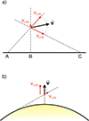 |
Fig. 4. Illustration of difference in LOS velocity components (i.e. velocity components projected along an incident ray) corresponding to various locations at the illuminating surface. |
To demonstrate the extent to which the narrow, velocity-sensitive spectral lines are affected by these factors, we use the Mg II k line as an example. For simplicity, we only assume the radial movement of the illuminated plasma away from the solar surface. We discuss the implications of more general dynamics in Sect. 5.
In Fig. 5, we show the disc-averaged profiles of the Mg II K line (solid lines) ‘seen’ by plasma at different altitudes when moving with different velocities. Here, it is important to note that our aim is to demonstrate the sensitivity only on the velocity and altitude. Therefore, we do not take the dilution factor into account. Applying corresponding dilution factors in Fig. 5 would cause a decrease in intensities with rising altitude, which would mask some of the behaviour we aim to study. The omission of the dilution factor is apparent from the disc-averaged profiles representing the static situation, which are plotted in each panel of Fig. 5 using dashed lines. By keeping these static profiles identical in each panel, we can better recognise the differences between the profiles resulting from each combination of altitude and velocity parameters. In Fig. 5, we assume altitudes of 5000 km, 10 000 km, 100 000 km, and 1RSun (plotted from left to right). The radial velocity values used here are 20 km s−1, 30 km s−1, 50 km s−1, 70 km s−1, and 100 km s−1 (plotted from top to bottom).
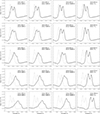 |
Fig. 5. Disc-averaged profiles of the Mg II K line (solid lines) seen by plasma at different altitudes when moving with different velocities. Altitudes: 5000 km, 10 000 km, 100 000 km, and 1RSun (from left to right). Radial velocities: 20 km s−1, 30 km s−1, 50 km s−1, 70 km s−1, and 100 km s−1 (from top to bottom). The static angle-averaged profile is plotted in each panel using the dashed line. We note that we do not take into account the dilution factor. |
Figure 5 shows that at low altitudes (below 10 000 km), a change in the shape of the incident radiation profiles – specifically in the height and asymmetry of the peaks, and the depth of the reversal – starts to be noticeable even with velocities of 20 km s−1. With velocities of 30 km s−1, the transformation of the profiles becomes significant. With velocities above 50 km s−1, the incident Mg II K profiles lose their double-peaked character and become strongly asymmetric. This complete transformation is also present at higher altitudes (around 100 000 km) with velocities over 70 km s−1. Only at altitudes above 1RSun does the resulting incident radiation profiles closely resemble the simply Doppler-shifted static profile, even with velocities over 100 km s−1.
The cause of the discrepancy between the low and high altitudes is the fact that from low altitudes, the solar surface does not appear as a point source, but as an extended illuminating surface. Different areas on this surface thus correspond to different LOS velocity components (Fig. 4) that result in the asymmetries in the angle-averaged incident radiation profiles. The lower the altitude, the larger the difference between the LOS velocity components for the disc centre and limb areas, and the more asymmetric the profiles become.
To illustrate the mechanism leading to the strong asymmetries in the Mg II K line, in Fig. 6 we show separate profiles from different areas on the solar disc, ranging from the disc centre to the limb. To do so, we assume ten concentric-ring zones with equal areas, covering the entire solar disc. The same zones were used by Gunár et al. (2021; see Fig. 2 therein). The spectral profiles corresponding to each zone (shown in Figs. 3 and 5 of Gunár et al. 2021) clearly illustrate the centre-to-limb variation. We take this variation into account and use the profiles corresponding to each zone as published by Gunár et al. (2021). For each zone, we derive the corresponding LOS velocity component for the altitude of 10 000 km and the velocity of 50 km s−1 and plot the Doppler-shifted profiles in the left panel of Fig. 6. There, the profile with the largest shift from the static case (dashed line) corresponds to the zone at the disc centre. The profile with the least Doppler shift corresponds to the zone at the limb. From Fig. 6, it is clear that the averaged profile from all zones (shown in the right panel) loses the double-peaked character and becomes highly asymmetric. This transformation is mainly due to the difference in the LOS velocity components corresponding to different regions on the solar disc, and to a lesser extent due to the centre-to-limb variation. We note that to produce the angle-averaged incident radiation profiles, we did not take into account the effect described in Sect. 3. This would only have a minor impact on the actual shape of the resulting profiles and would not affect our analysis and conclusions.
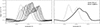 |
Fig. 6. Illustration of mechanism causing strong asymmetries in the incident radiation Mg II K line profiles received by moving plasma. This example is for a radial velocity of 50 km s−1 and altitude of 10 000 km. In the left panel are ten profiles corresponding to the solar-disc illumination from ten concentric-ring zones of Gunár et al. (2021). The profile with the largest shift from the static case (dashed lines) corresponds to the zone at the disc centre. The profile with the least Doppler shift corresponds to the zone at the limb. In the right panel is the averaged profile from all zones. |
5. Discussion
5.1. Altitude
From Table 1, we can see that the portion of the solar disc visible from low altitudes is very restricted. This has strong implications for the definition of incident radiation in any instance when we analyse specific spectroscopic observations of low-lying solar structures. This is because the limited field of view (e.g. 2.79% of the entire solar disk from an altitude of 20 000 km) is comparable to the size of active regions (e.g. Fludra & Ireland 2008; Tziotziou et al. 2014). This means that the entire field of view may be filled by a quiet-Sun area, but also by an active region or a coronal-hole region. However, this would lead to profoundly different intensities of the incident radiation. We may realistically expect the actual incident radiation to differ significantly more than the disk-averaged radiation during the minimum and maximum activity stages of the solar cycle. However, these variations already reached above 40% in the latest solar cycle for the Mg II K line (Koza et al. 2022; Gunár et al. 2022) and above 80% in previous cycles for the Lyman-α line (Gunár et al. 2020). Furthermore, the same argument can also be extended, even to larger altitudes. For example, at 50 000 km or 100 000 km, the visible portion of the solar surface covers only 6.71% and 12.57% of the solar disc, respectively. Active regions could still fill a large fraction of such a field of view, which is also comparable to the size of coronal holes (e.g. Heinemann et al. 2020).
Clearly, the difference between the incident radiation in various scenarios can be rather large, with a dramatic impact on the results of spectral inversions (see e.g. Gunár et al. 2020, 2022). However, even the determination of the correct incident radiation is not so straightforward. In the case when the observed structure ‘sees’ only the quiet Sun, the incident radiation is well represented by the reference quiet-Sun profiles; for example, those from Gunár et al. (2020, 2021). In contrast, there are no reference profiles derived specifically for active regions or coronal holes. We can expect reference profiles for fields of view mixing quiet-Sun and active-Sun regions even less. Therefore, to determine the relevant incident radiation boundary conditions, we may often need to specify them for each case of observations when high-precision spectral inversions are the goal. Such direct analysis of the disc portion visible to the observed structures and the determination of the relevant incident radiation was done, for example, by Dolei et al. (2019), Vial et al. (2019), and Zhang et al. (2019).
The situation is different in the case of high-altitude structures, such as eruptive prominences and the cores of coronal mass ejections (CMEs). From the altitude above 300 000 km, more than 30% of the solar disc illuminates the observed plasma. This portion rises to 50% at the altitude of 1RSun. Moreover, the higher the illuminated plasma travels (eruptive prominences were detected at altitudes reaching 6RSun; see for example Mierla et al. 2022; Russano et al. 2024), the larger the portion of the entire disc that illuminates it. These large fractions of the solar disc are statistically similar to the entire solar disc. Therefore, to determine the incident radiation at such altitudes, it is safe to assume the reference spectra adjusted to the corresponding stage of the solar cycle, as published, for example, by Gunár et al. (2020) and Koza et al. (2022).
5.2. Dynamics of the illuminated plasma
From Sect. 4, it is clear that the incident radiation received by moving plasma is strongly affected by its velocity, especially at lower altitudes. In the Mg II H&K lines, it is significantly affected by the presence of radial velocities as low as 30 km s−1. A similarly strong influence is also present in the case of the Lyman lines (Heinzel & Rompolt 1987; Gontikakis et al. 1997a) and to a lesser degree in the He I line (Labrosse et al. 2007). Such velocities are even observed in the fine structures of quiescent prominences (Labrosse et al. 2010; Vial & Engvold 2015) and are easily superseded by the velocities observed in the dynamic chromospheric and coronal structures. Therefore, the impact of dynamics on the shape of the incident radiation profiles may need to be considered in many situations when analysing observed chromospheric and coronal structures.
All examples of the impacts of velocities on the incident radiation profiles shown in this paper assume radially moving plasma. However, while the radial velocity component has the most pronounced influence, the horizontal velocities also affect the shapes of the incident radiation profiles. If we now assume plasma moving in the direction parallel to the solar surface, it is clear that the largest Doppler shift would be present in the radiation from the limb areas. At the same time, the radiation from the disc centre would not be shifted at all. This would again lead to asymmetry in the angle-averaged incident radiation profiles. The difference between the actual angle-averaged profiles and the static case would again depend on the altitude of the moving plasma, with the most pronounced differences being at the lowest altitudes. Moreover, the asymmetries of the incident radiation profiles would not be the same on all sides of the moving structures. Rather, there would be opposing values at the front and at the back of the structure (defined with respect to the direction of the movement). The implications of such an asymmetric illumination on the results of spectral (and spectro-polarimetric) inversions are not yet fully understood.
6. Conclusions
Our analysis of the influence of altitude on the definition of the incident radiation boundary conditions takes into account a wide range of altitudes. This way, we can encompass a diverse range of solar structures, from the high-rising eruptive prominences to the low-lying spicules. That allows us to conclude that the altitude of the illuminated plasma strongly differentiates the approach we need to take to define incident radiation accurately.
Structures – such as spicules or low-lying filaments – that do not reach high altitudes are illuminated by very limited portions of the solar disc. This field of view represents only 0.29% of the entire solar disc from an altitude of 2000 km, 0.71% from an altitude of 5000 km, and 2.79% from 20 000 km (see Table 1). As we discuss in Sect. 5.1, such small areas of the solar disc are comparable to the size of active regions or coronal holes. Therefore, the entire field of view may be, in general, filled with quiet-Sun areas, but also with an active region or a coronal hole. That would lead to a large discrepancy in the actual incident radiation. Therefore, to determine the correct incident radiation for low-lying structures, it is necessary to study the actual composition of the portion of the solar disc illuminating them. Such a direct determination of the incident radiation boundary conditions was done by Dolei et al. (2019), Vial et al. (2019), and Zhang et al. (2019), for example. Nevertheless, the direct determination of the incident radiation boundary conditions for structures located at the limb remains difficult. This is because we currently cannot simultaneously observe the structures at the limb and the solar disc areas surrounding them. The conditions on the solar disc can only be observed several days prior, or later, when the Sun rotates sufficiently to allow observations from the Earth direction. However, the high-fidelity direct determination of the incident radiation is generally not necessary for theoretical studies of the coronal and chromospheric structures using radiative-transfer modelling. Only when performing the high-precision spectral inversions of specific observed events should the level of accuracy discussed here be considered.
This situation is different for high-altitude structures, such as eruptive prominences or cores of CMEs. The fraction of the solar disc that illuminates these structures is large; for example, 50% at an altitude of 1RSun. Such a large area may be realistically assumed to be filled with a mixture of quiet-Sun and active-Sun areas in statistically similar proportion to the entire solar disc. Therefore, the reference spectra corresponding to the stage of the solar cycle in which the analysed event was observed will be sufficient to maintain the precision of spectral inversions.
The factor that will play a more important role in the spectral inversions of observations of eruptive prominences and CME cores is their significant dynamics. The influence of dynamics on the incident radiation received by fast-moving plasma was already shown by for example Heinzel & Rompolt (1987), Gontikakis et al. (1997b), and Labrosse et al. (2007) in the case of the Lyman-α, Lyman-β and Hα, and He I lines, respectively. As our example of the Mg II K line (Sect. 4) demonstrates, incident radiation in narrow, velocity-sensitive spectral lines is affected by radial velocities as low as 30 km s−1. This means that to achieve high precision of spectral inversions of observations in lines such as Mg II H&K or Ca II H&K, the impact of the dynamics should be considered in any instance when such velocities are present.
At this point, it is important to note that any improvement in the accuracy of the definition of the incident radiation boundary conditions requires a good understanding of the basic properties of the radiation in a given spectral line emerging from the solar disc – such as its disc-averaged profile and the nature of its centre-to-limb variation. For the spectral lines playing the dominant role in the illumination of the coronal and chromospheric structures, the most recent incident radiation data can be found in the following works. The disc-averaged reference profiles of the Lyman-α line were published by Gunár et al. (2020). This line does not exhibit any clear sign of the centre-to-limb variation, as was shown by Curdt et al. (2008). The quiet-Sun reference profiles of the Mg II H&K lines and their centre-to-limb variation were studied by Gunár et al. (2021). Quiet-Sun spectra and the centre-to-limb variation of the Ca II H&K and 8542 Å lines, together with other lines in the optical spectral range, were presented by Pietrow et al. (2023). The reference profiles of the higher Lyman lines (above Lyman-α) can be found in Warren et al. (1998). The quiet-Sun profiles of the Hα line are typically obtained from David (1961).
In the present work, we only focused on the illumination in spectral lines from the solar disc. However, spectral inversions also depend on the illumination in various continua as well as on the illumination from the corona. For example, the helium photoionization in prominences depends on illumination from both the solar disc and corona. The latter is prominent below 504 Å due to a forest of extreme ultra-violet (EUV) coronal lines. Another important aspect is that illumination in the Lyman lines and continuum determines the internal radiation field in these transitions, and this radiation field then ionises Mg II to Mg III and Ca II to Ca III. This means that the partial ionisation of magnesium or calcium is dependent on the illumination in the Lyman transitions (see e.g. Heinzel et al. 2024).
The goal of the current work is not to perform spectral inversions using any particular model. Rather, we focused on two aspects of the incident radiation boundary conditions that are relevant for spectral inversions based on any kind of modelling approach. Both aspects -the altitude above the solar surface and the dynamics of the plasma- play a role in the definition of the incident radiation for 1D, 2D, or 3D models alike. In fact, the choice of the model geometry, such as 1D slabs compared to 3D multi-structure simulations, likely has a more significant impact on the precision of spectral inversions than the definition of illumination. A similar impact could be expected from the choice of the details of radiative transfer calculations employed in spectral inversions (e.g. complete or partial frequency distribution, assumption of statistical equilibrium or non-equilibrium ionization, etc). Such comparisons are, however, beyond the scope of the current paper. Nevertheless, the results presented here will help to improve the definition of the incident radiation boundary conditions for any modelling used for spectral inversions.
Acknowledgments
S.G. and P.H. acknowledge the support from grant 22-34841S of the Czech Science Foundation (GAČR). P.H. was supported by the program “Excellence Initiative–Research University” for the years 2020–2026 at the University of Wrocław, project No. BPIDUB.4610.96.2021.KG. S.G. and P.H. acknowledge the support from the project RVO:67985815 of the Astronomical Institute of the Czech Academy of Sciences.
References
- Barczynski, K., Schmieder, B., Peat, A. W., et al. 2021, A&A, 653, A94 [NASA ADS] [CrossRef] [EDP Sciences] [Google Scholar]
- Curdt, W., Tian, H., Teriaca, L., Schühle, U., & Lemaire, P. 2008, A&A, 492, L9 [NASA ADS] [CrossRef] [EDP Sciences] [Google Scholar]
- da Silva Santos, J. M., de la Cruz Rodríguez, J., Leenaarts, J., et al. 2020, A&A, 634, A56 [NASA ADS] [CrossRef] [EDP Sciences] [Google Scholar]
- David, K.-H. 1961, ZAp, 53, 37 [Google Scholar]
- De Pontieu, B., Title, A. M., Lemen, J. R., et al. 2014, Sol. Phys., 289, 2733 [Google Scholar]
- Dolei, S., Spadaro, D., Ventura, R., et al. 2019, A&A, 627, A18 [NASA ADS] [CrossRef] [EDP Sciences] [Google Scholar]
- Fludra, A., & Ireland, J. 2008, A&A, 483, 609 [NASA ADS] [CrossRef] [EDP Sciences] [Google Scholar]
- Gontikakis, C., Vial, J.-C., & Gouttebroze, P. 1997a, Sol. Phys., 172, 189 [NASA ADS] [CrossRef] [Google Scholar]
- Gontikakis, C., Vial, J.-C., & Gouttebroze, P. 1997b, A&A, 325, 803 [NASA ADS] [Google Scholar]
- Gunár, S., Schwartz, P., Koza, J., & Heinzel, P. 2020, A&A, 644, A109 [EDP Sciences] [Google Scholar]
- Gunár, S., Koza, J., Schwartz, P., Heinzel, P., & Liu, W. 2021, ApJS, 255, 16 [CrossRef] [Google Scholar]
- Gunár, S., Heinzel, P., Koza, J., & Schwartz, P. 2022, ApJ, 934, 133 [CrossRef] [Google Scholar]
- Heinemann, S. G., Jerčić, V., Temmer, M., et al. 2020, A&A, 638, A68 [EDP Sciences] [Google Scholar]
- Heinzel, P. 1983, Bull. Astron. Inst. Czechoslovakia, 34, 1 [Google Scholar]
- Heinzel, P., & Rompolt, B. 1987, Sol. Phys., 110, 171 [NASA ADS] [CrossRef] [Google Scholar]
- Heinzel, P., Susino, R., Jejčič, S., Bemporad, A., & Anzer, U. 2016, A&A, 589, A128 [NASA ADS] [CrossRef] [EDP Sciences] [Google Scholar]
- Heinzel, P., Berlicki, A., Bárta, M., et al. 2022, ApJ, 927, L29 [NASA ADS] [CrossRef] [Google Scholar]
- Heinzel, P., Gunár, S., & Jejčič, S. 2024, Philos. Trans. A, 382, 20230221 [NASA ADS] [Google Scholar]
- Jejčič, S., & Heinzel, P. 2009, Sol. Phys., 254, 89 [NASA ADS] [CrossRef] [Google Scholar]
- Jejčič, S., Heinzel, P., Schmieder, B., et al. 2022, ApJ, 932, 3 [CrossRef] [Google Scholar]
- Koza, J., Kuridze, D., Heinzel, P., et al. 2019, ApJ, 885, 154 [NASA ADS] [CrossRef] [Google Scholar]
- Koza, J., Gunár, S., Schwartz, P., Heinzel, P., & Liu, W. 2022, ApJS, 261, 17 [NASA ADS] [CrossRef] [Google Scholar]
- Labrosse, N. 2015, in Solar Prominences, eds. J. C. Vial, & O. Engvold, Astrophys. Space Sci. Lib., 415, 131 [NASA ADS] [CrossRef] [Google Scholar]
- Labrosse, N., Gouttebroze, P., & Vial, J.-C. 2007, A&A, 463, 1171 [NASA ADS] [CrossRef] [EDP Sciences] [Google Scholar]
- Labrosse, N., Heinzel, P., Vial, J., et al. 2010, Space Sci. Rev., 151, 243 [CrossRef] [Google Scholar]
- López Ariste, A. 2015, in Astrophysics and Space Science Library, eds. J. C. Vial, & O. Engvold, Astrophys. Space Sci. Lib., 415, 179 [CrossRef] [Google Scholar]
- Mierla, M., Zhukov, A. N., Berghmans, D., et al. 2022, A&A, 662, L5 [NASA ADS] [CrossRef] [EDP Sciences] [Google Scholar]
- Peat, A. W., Labrosse, N., Schmieder, B., & Barczynski, K. 2021, A&A, 653, A5 [NASA ADS] [CrossRef] [EDP Sciences] [Google Scholar]
- Peat, A. W., Labrosse, N., & Gouttebroze, P. 2023, A&A, 679, A156 [NASA ADS] [CrossRef] [EDP Sciences] [Google Scholar]
- Pietrow, A. G. M., Kiselman, D., Andriienko, O., et al. 2023, A&A, 671, A130 [NASA ADS] [CrossRef] [EDP Sciences] [Google Scholar]
- Ruan, G., Jejčič, S., Schmieder, B., et al. 2019, ApJ, 886, 134 [NASA ADS] [CrossRef] [Google Scholar]
- Russano, G., Andretta, V., De Leo, Y., et al. 2024, A&A, 683, A191 [NASA ADS] [CrossRef] [EDP Sciences] [Google Scholar]
- Sainz Dalda, A., de la Cruz Rodríguez, J., De Pontieu, B., & Gošić, M. 2019, ApJ, 875, L18 [Google Scholar]
- Tziotziou, K., Tsiropoula, G., Georgoulis, M. K., & Kontogiannis, I. 2014, A&A, 564, A86 [NASA ADS] [CrossRef] [EDP Sciences] [Google Scholar]
- Vial, J. C., & Engvold, O. 2015, in Solar Prominences, Astrophys. Space Sci. Lib., 415 [Google Scholar]
- Vial, J. C., Zhang, P., & Buchlin, É. 2019, A&A, 624, A56 [NASA ADS] [CrossRef] [EDP Sciences] [Google Scholar]
- Warren, H. P., Mariska, J. T., & Wilhelm, K. 1998, ApJS, 119, 105 [Google Scholar]
- Zhang, P., Buchlin, É., & Vial, J. C. 2019, A&A, 624, A72 [NASA ADS] [CrossRef] [EDP Sciences] [Google Scholar]
All Tables
All Figures
|
Fig. 1. Geometry of situation in which a structure located at an altitude of 100 000 km receives illumination from the solar surface. The arc length of dmax corresponds to the maximum visible distance from the given altitude. |
| In the text | |
|
Fig. 2. Illustration of extent of solar surface from which structures at altitudes of 10 000 km, 20 000 km, 30 000 km, 50 000 km, and 100 000 km receive illumination. The background image is a full-Sun mosaic obtained on 2019 October 20 in the Mg II K line centre by the Interface Region Imaging Spectrograph (IRIS; De Pontieu et al. 2014). |
| In the text | |
|
Fig. 3. Geometry of situation in which a structure located at an altitude of RSun receives illuminations from the solar surface. |
| In the text | |
|
Fig. 4. Illustration of difference in LOS velocity components (i.e. velocity components projected along an incident ray) corresponding to various locations at the illuminating surface. |
| In the text | |
|
Fig. 5. Disc-averaged profiles of the Mg II K line (solid lines) seen by plasma at different altitudes when moving with different velocities. Altitudes: 5000 km, 10 000 km, 100 000 km, and 1RSun (from left to right). Radial velocities: 20 km s−1, 30 km s−1, 50 km s−1, 70 km s−1, and 100 km s−1 (from top to bottom). The static angle-averaged profile is plotted in each panel using the dashed line. We note that we do not take into account the dilution factor. |
| In the text | |
|
Fig. 6. Illustration of mechanism causing strong asymmetries in the incident radiation Mg II K line profiles received by moving plasma. This example is for a radial velocity of 50 km s−1 and altitude of 10 000 km. In the left panel are ten profiles corresponding to the solar-disc illumination from ten concentric-ring zones of Gunár et al. (2021). The profile with the largest shift from the static case (dashed lines) corresponds to the zone at the disc centre. The profile with the least Doppler shift corresponds to the zone at the limb. In the right panel is the averaged profile from all zones. |
| In the text | |
Current usage metrics show cumulative count of Article Views (full-text article views including HTML views, PDF and ePub downloads, according to the available data) and Abstracts Views on Vision4Press platform.
Data correspond to usage on the plateform after 2015. The current usage metrics is available 48-96 hours after online publication and is updated daily on week days.
Initial download of the metrics may take a while.