| Issue |
A&A
Volume 687, July 2024
|
|
|---|---|---|
| Article Number | A189 | |
| Number of page(s) | 13 | |
| Section | Stellar atmospheres | |
| DOI | https://doi.org/10.1051/0004-6361/202449476 | |
| Published online | 12 July 2024 | |
Stellar Population Astrophysics (SPA) with the TNG
Measurement of the He I 10 830 Å line in the open cluster Stock 2★
1
Department of Astronomy, Stockholm University, AlbaNova University centre,
Roslagstullsbacken 21,
114 21
Stockholm,
Sweden
e-mail: mingjie.jian@astro.su.se
2
Department of Astronomy, School of Science, The University of Tokyo,
7-3-1 Hongo, Bunkyo-ku,
Tokyo
113-0033,
Japan
3
Purple Mountain Observatory, Chinese Academy of Sciences,
Nanjing
210023,
PR China
e-mail: xiaoting.fu@pmo.ac.cn
4
INAF – Osservatorio di Astrofisica e Scienza dello Spazio di Bologna,
via P. Gobetti 93/3,
40129
Bologna,
Italy
5
Department of Physics, University of Rome Tor Vergata,
via della Ricerca Scientifica 1,
00133
Rome,
Italy
6
INAF – Osservatorio Astronomico di Padova,
Vicolo dell’ Osservatorio 5,
35122
Padova,
Italy
7
National Astronomical Observatory of Japan,
2-21-1 Osawa, Mitaka,
Tokyo
181-8588,
Japan
8
INAF – Osservatorio Astrofisico di Arcetri,
Largo E. Fermi 5,
50125
Firenze,
Italy
9
INAF – Osservatorio Astrofisico di Catania,
via S. Sofia 78,
95123
Catania,
Italy
Received:
2
February
2024
Accepted:
13
April
2024
The precise measurement of stellar abundances plays a pivotal role in providing constraints on the chemical evolution of the Galaxy. However, before spectral lines can be employed as reliable abundance indicators, particularly for challenging elements such as helium, they must undergo thorough scrutiny. Galactic open clusters, representing well-defined single stellar populations, offer an ideal setting for unfolding the information stored in the helium spectral line feature. In this study, we characterise the profile and strength of the helium transition at around 10 830 Å (He 10 830) in nine giant stars in the Galactic open cluster Stock 2. To remove the influence of weak blending lines near the helium feature, we calibrated their oscillator strengths (log 𝑔f) by employing corresponding abundances obtained from simultaneously observed optical spectra. Our observations reveal that the He 10 830 in all the targets is observed in absorption, with line strengths categorised into two groups. Three stars exhibit strong absorption, including a discernible secondary component, while the remaining stars exhibit weaker absorption. The lines are in symmetry and align with or near their rest wavelengths, suggesting a stable upper chromosphere without a significant systematic mass motion. We find a correlation between the He 10 830 strength and the Ca II log R′HK index, with a slope similar to that reported in previous studies on dwarf stars. This correlation underscores the necessity of accounting for the stellar chromosphere structure when employing He 10 830 as a probe for the stellar helium abundance. The procedure of measuring the He 10 830 we developed in this study is applicable not only to other Galactic open clusters but also to field stars, and we plan to use it to map the helium abundance across various types of stars in the future.
Key words: line: profiles / stars: atmospheres / stars: chromospheres / stars: fundamental parameters / open clusters and associations: individual: Stock 2
Based on observations made with the Italian Telescopio Nazionale Galileo (TNG) operated on the island of La Palma by the Fundación Galileo Galilei of the INAF (Istituto Nazionale di Astrofisica) at the Spanish Observatorio del Roque de los Muchachos. This study is part of the Large Programme entitled Stellar Population Astrophysics (SPA): this study of the detailed, age-resolved chemistry of the Milky Way disc (A37TAC_31, PI: L. Origlia) started in 2018 and was granted observing time with HARPS-N and GIANO-B echelle spectrographs at the TNG.
© The Authors 2024
 Open Access article, published by EDP Sciences, under the terms of the Creative Commons Attribution License (https://creativecommons.org/licenses/by/4.0), which permits unrestricted use, distribution, and reproduction in any medium, provided the original work is properly cited.
This article is published in open access under the Subscribe to Open model. Subscribe to A&A to support open access publication.
1 Introduction
Recent measurements of the stellar elemental abundance ratio for stars in our Milky Way have provided valuable insights into the formation and evolution of our Milky Way and its sub-systems. Notably, studies have revealed that almost all globular clusters have multiple groups of stars with varying sodium and oxygen abundances, most probably because they formed in slightly different epochs (see e.g. Gratton et al. 2019), although some doubts as to the reality of subsequent generations remain (see e.g. Bastian & Lardo 2018). There is also indirect evidence from photometry or CN line measurements that the helium abundance varies within these stars (see e.g. Lee et al. 2005; Piotto et al. 2007; Bragaglia et al. 2010). Helium, as the second most abundant element in the Universe and the main product of hydrogen fusion in stellar nucleosynthesis, can serve as a tracer of the evolution of stars, clusters, and galaxies.
However, directly measuring the He abundances of stars from their spectra is difficult. For stars hotter than ~8500K, a few helium lines form in their photosphere (see e.g. Villanova et al. 2009). For cooler stars, determining the helium abundance is challenging due to the low temperatures (and thus low thermal energy) in their photosphere, which prevent the formation of these lines since the populations of the lower levels of the corresponding transitions are small.
One particular helium spectral line, located at around 10 830 Å (hereafter referred to as He 10 830), corresponds to the transition between the 2s and 2p triplet levels and can be observed in most late-type stars. The triplet involves the excitation of an electron in the 2s3S state of helium to one of the three excited states in the 2p3P manifold, with the excitation potential ~1.2eV (Ryabchikova et al. 2015): 2s3S -> 2p3P0 (λ = 10 829.09 Å), 2s3S -> 2p3P1 (λ = 10 830.25 Å), and 2s3S ->2p3P2 (λ = 10830.34 Å).
The strength of this He I line, which is quantitatively represented by its equivalent width (EW), depends on the population of the lower state (2s). As in cool stars, the flux of the high-energy photons in the photospheric radiation field is too low to efficiently populate the lower level of the transition. Thus, the line must be formed in an outer atmospheric layer with a higher temperature (i.e. an upper chromosphere), and other excitation mechanisms must be at work. Previous studies (Hirayama 1971; Zirin 1975; Zarro & Zirin 1986; Avrett et al. 1994) suggested that the photoionisation recombination mechanism, in which helium atoms are ionised by high-energy photons and subsequently recombine into triplet states, can populate the lower state of He 10 830. On the other hand, col-lisional excitation can directly excite atoms from singlet levels to triplet levels if the electron temperature in the atmosphere (Te) exceeds 20 000 K (Athay & Menzel 1956; Andretta & Jones 1997). In the case of a collisional excitation regime, the strength of He 10 830 is expected to be related to the chromosphere structure, which can be probed by diagnostics of the chromosphere as the cores of Ca II H&K lines. Moreover, we expect a correlation with diagnostics of magnetic activity at diverse atmospheric layers, such as the X-ray luminosity, which traces the coronal emission.
The complex formation mechanisms involved make it challenging to establish the relationship between the strength of He 10 830 and the stellar parameters, particularly the helium abundance (e.g. Dupree & Avrett 2013). Consequently, it remains difficult to accurately measure the helium abundance using the strength of the He 10 830 transition. Therefore, there is an urgent need to investigate and determine the elusive connection between the He 10 830 strength and other stellar parameters to enable spectroscopic measurements of the helium abundance in cool stars.
Many studies have been based on observations of the He 10 830 of cool stars and investigated its strength. Some early investigations (e.g. Vaughan & Zirin 1968; Zirin 1976; Smith 1983; Obrien & Lambert 1986) acquired low-resolution spectra of He 10 830 for a substantial number of stars. Zirin (1982) established an empirical relation between the line strength and various stellar parameters, including the effective temperature (Teff), Ca II K line intensity, and X-ray luminosity. These findings were subsequently confirmed by studies such as Zarro & Zirin (1986) and Takeda & Takada-Hidai (2011). With the development of near-infrared (NIR) high-resolution spectrographs, He 10 830 studies have entered the high-resolution era. The resolution around the He 10 830 line can reach Δλ ~ 0.2 Å or even smaller, allowing for much more detailed investigations of spectral features (see e.g. Smith et al. 2004, 2012; Sanz-Forcada & Dupree 2008; Dupree et al. 2009; Pasquini et al. 2011). However, variations in measurement techniques, such as profile fitting versus direct pixel summation, and the presence or absence of telluric line corrections can introduce systematic or statistical uncertainties when comparing results from different studies. Therefore, it is crucial to re-examine the empirical relations established over 40 years ago by Zirin (1982) with high-resolution spectrographs.
For the relation between the He 10 830 line strength and Ca II H&K line emissions (λ ~ 3931–3970 Å), obtaining spectra that simultaneously cover these lines is crucial to account for possible variations in the level of stellar activities and avoid potential biases. In this study, the first in a series of works probing helium abundances, we established a method for accurately measuring the strength and profile of the He 10 830 line based on high-resolution spectra obtained using the Telescopio Nazionale Galileo (TNG). We applied this method to a set of similar stars within a single stellar population, specifically red clump (RC) stars in the open cluster Stock 2.
Stock 2 is a nearby open cluster discovered by Stock (1956), at a distance of 400 pc (Dib et al. 2018). Its age and chemical composition were not well known until recently. The first detailed spectroscopic analysis of this cluster was reported by Reddy & Lambert (2019). With a sample of three giants, they estimated the cluster’s iron abundance value ([Fe/H]) to be −0.06 ± 0.03. Ye et al. (2021) obtained a similar value of −0.04 ± 0.15 from the medium-resolution spectra of around 300 stars obtained by The Large Sky Area Multi-Object Fibre Spectroscopic Telescope (LAMOST; Cui et al. 2012). As a part of the TNG Large Programme Stellar Population Astrophysics (SPA; see e.g. Origlia et al. 2019; Casali et al. 2020; Zhang et al. 2021), Alonso-Santiago et al. (2021) analysed the spectra of 32 dwarfs, 14 main sequence turnoff (MSTO) stars, and ten giants, and derived their stellar parameters and chemical abundances. They conclude that the age and iron abundance of the cluster are 450 Myr and [Fe/H]=−0.07 ± 0.06. As the member stars have similar ages and chemical compositions, this is an ideal sample for studying the behaviour of helium lines in a given stellar population.
We outline the observations and explain the data reduction process in Sect. 2. Section 3 focuses on characterising the blending of He 10 830. In Sect. 4, we describe the methods used to measure He 10 830 and Ca II H&K lines. Finally, we present the results and a discussion in Sect. 5.
2 Data and reduction
The data used in this study consist of high-resolution NIR and optical spectra of 9 giants in the open cluster Stock 2, obtained as a part of the SPA project. The data used here for Stock 2 were observed in the GIARPS mode (Claudi et al. 2017) at the TNG. GIARPS combines the GIANO-B (Oliva et al. 2006) for obtaining NIR spectra (0.9–2.45 µm) with a resolution of R = 50 000, and the HARPS-N (Cosentino et al. 2012) for obtaining optical spectra (0.383–0.690 µm) with R = 115 000, simultaneously capturing the required spectral ranges. The simultaneous observation of Ca II H&K lines using HARPS-N and He 10 830 lines with GIANO-B provides a direct comparison of their behaviour. This is particularly valuable as it enables the avoidance of any potential time-dependent variations between these lines.
The age, iron abundance (as a proxy of metallicity), differential reddening, and chemical abundances of Stock 2 stars are reported in Alonso-Santiago et al. (2021) based on the HARPS-N data of our GIARPS observations. We followed the naming convention from Table 1 of Alonso-Santiago et al. (2021) and present the target list in Table 1, as well as the stellar parameters in Table 2. Figure 1 shows the Gaia DR2 colour-magnitude diagram (CMD) of our targets, along with the other member stars from Cantat-Gaudin et al. (2018). The PARSEC isochrone version 1.2S1 (Bressan et al. 2012) with an age of 450 Myr, a metallicity of [M/H]=−0.07, and an extinction of AV = 0.84 is overplotted as a reference. We selected the Gaia DR2 photometric system from the PARSEC CMD 3.7 web page for the isochrone with the bolometric correction from YBC (Chen et al. 2019). The isochrone parameters were adopted from Alonso-Santiago et al. (2021). We note that the scatter of the RC stars and the extended main sequence are mainly due to the differential reddening in this cluster (see the detailed discussions in Alonso-Santiago et al. 2021).
While we lack the precise asteroseismic data needed to robustly distinguish between red giant branch (RGB) and RC stars, we are confident that our sample stars are most likely RC stars. This confidence stems not only from their placement within a relatively narrow range of colour and absolute magnitude, but also from the probabilistic nature of observations. The turnoff mass of Stock 2 is about 2.8 M⊙ (Alonso-Santiago et al. 2021). Stars with this mass evolve very fast along the sub-giant branch and RGB, making them challenging to capture in observation samples. In contrast, stars in this mass range spend a more considerable amount of time in the RC stage. As a result, these RC stars have a substantially higher probability of being sampled in observations. This increased sampling probability, combined with the constraints of colour and absolute magnitude, strongly suggests that our sample stars are predominantly RC stars.
We aimed to measure He 10 830 in RC stars because their surface helium abundances are expected to be the same. This expectation arises from the assumption that within a single stellar population, such as an open cluster, Stock 2 in our case, the surface helium abundance remains relatively consistent for RC stars. In Fig. 2, we present the surface He mass fraction (Y) in a single stellar population characterised by the metallicity of Stock 2. The PARSEC isochrone used here aligns with the one employed in Fig. 1, which includes the surface helium content evolution. To gauge the stage of stellar evolution, we used the surface gravity log (𝑔) as an indicator. During the main sequence phase, the surface helium mass fraction Y decreases (see the evolutionary phase with log (𝑔) ⪆ 4 in the figure) due to microscopic diffusion. The Microscopic diffusion leads the surface abundance decrease for elements heavier than hydrogen. For the microscopic diffusion treatments in stellar models and its impact on the surface elemental abundances, we recommend the PAR-SEC modelling paper (e.g. Bressan et al. 2012; Fu et al. 2015) for more detailed discussions. This decrease in Y is later counterbalanced by the first dredge-up at the end of the main sequence, restoring Y to its initial value, Y0. This restoration is evident in the range of log (𝑔) ≈ 4 to the MSTO. The surface He abundance of main sequence stars in Stock 2 is strongly affected by the microscopic diffusion. However, giant stars in Stock 2, with an approximate mass of 2.8 M⊙, undergo a negligible microscopic diffusion during their main sequence, attributed to their narrow surface convective zone. In the subsequent sub-giant branch phase, from the MSTO to the RGB onset, the surface He content remains consistent with the initial value Y0. The onset of the RGB phase is marked by the merging of the hydrogen-burning shell and the stellar surface convective zone, leading to a rapid increase in surface Y due to the transportation of fresh helium from the hydrogen-burning shell. This increase continues up to the tip of the RGB. In the subsequent RC phase (highlighted by red-filled dots in the figure), stars share a similar stellar structure and exhibit a nearly constant surface helium content. This uniformity in surface He abundance means that variations in the He 10 830 line observed in these RC stars predominantly reflect the local chromospheric conditions, where this spectral line is formed. While sub-giant phase stars also exhibit similar surface helium levels, their rapid evolution makes them challenging to sample in observations. As main sequence and RGB stars in the cluster experience either a decrease or increase in surface He abundance, measuring He 10 830 in RC stars effectively eliminates additional uncertainties that might arise from variations in the He abundance itself.
The reduction of the GIANO-B spectra was carried out using the data reduction pipeline software GOFIO (Rainer et al. 2018). This pipeline applied the needed corrections to the observed frames, namely the removal of bad pixels and cosmic rays, subtraction of sky and dark frame, and correction of flat-field and blaze. The normalised 1D spectra were then extracted by the pipeline and wavelength calibrated. The telluric lines – the spectral lines that originated from the Earth’s atmosphere instead of the stellar atmosphere – are also present in these extracted spectra. We used a python package, telfit2 (Gullikson et al. 2014), to fit the telluric lines and then subtract them from the observed spectra. A new continuum normalisation was performed after the subtraction. These corrected spectra were used for the measurement of the stellar and line parameters in Sect. 3. We note that such a procedure of telluric correction may alter the shape of He 10 830 in some cases. Thus, for the measurement of He 10 830, instead of using the telluric corrected spectra, all lines around 10 830 Å were fitted, including the telluric lines (see Sect. 4.1 for more detail). Figure 3 shows an example of He 10 830. To evaluate the stellar activity of our sample stars, we used the same set of HARPS-N spectra as in the research by Alonso-Santiago et al. (2021). The normalisation process and line measurement is described in Sect. 4.2.
Observation log.
Stellar parameters of our targets.
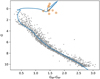 |
Fig. 1 CMD in Gaia DR2 photometry bands of Stock 2 member stars (grey) from Cantat-Gaudin et al. (2018), with the sample stars in this study marked with orange circles. The PARSEC isochrone with an age of 450 Myr, [M/H] = −0.07 and an extinction of AV = 0.84 is overplotted in blue. |
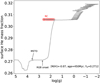 |
Fig. 2 He mass fraction (Y) on the stellar surface as a function of surface gravity, log (𝑔), for the Stock 2 isochrone. The initial He mass fraction of this isochrone is Y0 = 0.2712. The locations of the MSTO, RGB onset, and RC phase are highlighted. |
3 Blending around He 10 830
The presence of line blending, where spectral lines overlap in wavelength, can significantly alter the shape and strength of our target line, particularly when it is wide and weak. If we measure the strength of He 10 830 without accounting for the blending from the nearby spectral lines, the line strength would be over-estimated. Consequently, determining the extent of line blending around the He 10 830 for our target stars is necessary before accurately measuring the strength of He 10 830 can be achieved. By comparing observed spectra with synthetic spectra, we can disentangle the contributions of He 10 830 and other spectral lines, allowing for a more precise evaluation of the blending effects. Figure 3 presents the synthetic spectra around He 10 830 (excluding the helium feature) for star g1 in our sample. The synthetic spectra are generated using the local ther-modynamic equilibrium radiative transfer code MOOG (version November 2019; Sneden et al. 2012) with the ATLAS9 stellar atmosphere model from Castelli & Kurucz (2003) and the line list from Vienna Atomic Line Database (VALD3; without hyper-fine structure; Ryabchikova et al. 2015)3. The VALD3 database provides a comprehensive line list on our target wavelengths.
The prominent atomic lines around He 10 830 are marked with black arrows in Fig. 3. The figure clearly illustrates the presence of numerous atomic lines, such as Ca I, Fe I, and Si I which contaminate the He 10 830 line region. Therefore, it is crucial to account for these lines when measuring the EW of He 10 830 to ensure accurate results. Their contributions need to be carefully considered and taken into account in the analysis.
The observed spectra reveal that these lines are weaker than they appear in the synthetic spectra. This discrepancy exceeds the range of errors associated with the parameters such as Teff, log(𝑔), metallicity, or elemental abundances. The most likely cause of this difference is the incorrect atomic parameters of the line, particularly the log𝑔f in the infrared region. As demonstrated by Andreasen et al. (2016) with the solar spectrum, incorrect log 𝑔f values obtained from VALD3 can result in more than one dex discrepancies in the abundances of certain NIR Fe lines, even when using the same solar atmosphere model parameters. To address this issue, they proposed a list of calibrated log 𝑔f values based on solar abundances. The blending lines around the He 10 830 region in our sample stars face a similar challenge. These lines’ log 𝑔f values need to be calibrated using the observed spectra before accurately assessing their contribution to the He 10 830 line. The high resolution and high signal-to-noise ratio of the GIANO-B spectra obtained for Stock 2 makes them an ideal sample for such calibration efforts.
We started our calibration by determining the global stellar parameters that affect the line shape and strength, mainly the microturbulence velocity of a Gaussian profile, ξ, and the broadening velocity, Vbroad. We then used the elemental abundance derived from the HARPS-N spectra, which are observed simultaneously, to calibrate the log 𝑔f values of each blending line.
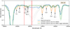 |
Fig. 3 Observed (blue step line; with telluric correction) and the synthetic spectra before (orange) and after (green) their log 𝑔f values are calibrated (without the He 10 830) for star g1. Vertical dashed red lines indicate the position of the He 10 830 triplet, and the black arrows indicate the position of blending lines with log 𝑔f values calibrated (see Sect. 3). The spectra of the other eight target stars are plotted in grey as a reference. |
3.1 Measurement of ξ and broadening velocity
Microturbulence velocity ξ represents the small-scale non-thermal motion in the stellar atmosphere. It mainly affects the strength of the saturated lines. Broadening velocity is an indicator of the combination of larger-scale non-thermal motion, or macroturbulence, and stellar rotation. These two parameters, along with Teff, log (𝑔), metallicity and elemental abundances, are the main factors that alter the spectral line. Alonso-Santiago et al. (2021) determined the values of Teff, log (𝑔), [Fe/H] and elemental abundances for our sample stars using the ROTFIT code.
However, ROTFIT does not yield values for microturbulence velocity (ξ). Instead, it adopts the microturbulence and macro-turbulence from template spectra, and calculates the projected rotational velocity (v sin i). To conduct a detailed characterisation of the He 10 830 line features, in this work we determined ξ and the broadening velocity, Vbroad, for our sample stars using the GIANO-B spectra.
We followed the approach described in Kondo et al. (2019) to determine ξ and Vbroad. It is summarised in two steps: (i) select isolated Fe I lines in the GIANO-B wavelength range, and (ii alter ξ, [Fe/H], and Vbroad to fit the observed spectra using the MPFIT algorithm (Takeda 1995).
In the first step, the isolated Fe I lines are defined as those with clear detectable absorption (depth d > 0.05) at the signal-to-noise ratio (S/NHe 10 830) of our sample and a small overlap with any other eventual line, whose depth must be less than 20% at the line centre. We avoided the regions with strong telluric absorption, such as 11 060–11 550 Å, 13 150–15 150 Å, 17 600– 21 000 Å, and > 23 500 Å. Such criteria yield 179 Fe I lines from 9820 to 22 473 Å.
In the second step, the observed spectra (those with the instrumental broadening from GIANO) for all the lines selected in step one are fit by choosing the ξ value so that the line-by-line [Fe/H] is not dependent on the line strength. The fitting of Vbroad is added during this process to provide a better fit between the observed and synthetic spectra. [Fe/H] is also determined in step two, which provides a good comparison to the value determined from the optical (HARPS-N) spectra.
A bootstrap method was then used to determine the parameters together with their uncertainties for each star. We chose 179 lines randomly from those selected in step (i) but allowed repeat selection (i.e. some lines are selected more than one time while others may be discarded), and apply MPFIT using these lines for a star. This procedure is then repeated 1000 times, and the final values, as well as the errors of ξ, [Fe/H], and Vbroad are set as the median and standard deviation of the obtained results. Table 2 lists these parameters for our sample. The derived ξ values are consistent with the trend reported by Holtzman et al. (2018) from the APOGEE giants, and the precision of the metallicities measured using the GIANO-B spectra is similar to those obtained from the HARPS spectra, as shown in Fig. 4. The measured Vbroad are around 5.5 km s−1. This is in perfect agreement with the low values found by Alonso-Santiago et al. (2021), who measured a v sin i of less than 4 km s−1 (on average) for the giants in Stock 2.
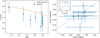 |
Fig. 4 Measured stellar parameters. Left panel: measured ξ from MPFIT versus log (𝑔) for the Stock 2 stars, along with the relation reported in Holtzman et al. (2018). Right panel: [Fe/H] values determined from GIANO-B spectra versus those from HARPS-N (Alonso-Santiago et al. 2021), with the histogram of Δ[Fe/H] = [Fe/H]GIANO-B ~ [Fe/H]harps-n in the upper-left corner. |
3.2 log gf calibration of blending lines
With all the global parameters that affect the line strength determined in the above section, the log 𝑔f values of the blending lines around He 10 830 are now ready to be calibrated. The strongest lines in the synthetic spectrum near He 10 830, which are indicated by black arrows in Fig. 3 and reported in Table 3, were selected to be calibrated. Other lines are found to have a negligible contribution using the synthetic spectra, with a maximum depth of less than 0.01 for our sample stars. The strong Si I line at 10 827.088 Å on the left side of He 10 830 was not included for calibration due to its potential impact on the wing of He 10 830. It was be treated during the fitting of He 10 830 (Sect. 4.1).
The log 𝑔f values of these lines were then adjusted to find the best fit between the synthetic and observed spectra, starting with the strongest line. Here we adopted the Si, Ca, Ti, and Fe abundance ratios from Alonso-Santiago et al. (2021). Calibration results were discarded if the line was affected by remaining telluric absorption (i.e. the Fe I line at 10 833.96 Å) or if they were affected by He 10 830 (i.e. the Ca I, Fe II, and Si I lines at around 10 829.50 Å). The final log 𝑔f value for each line is set as the median of the log 𝑔f values from all the stars. The values before and after the calibration are presented in Table 3 and the synthetic spectra for star g1 are shown in Fig. 3. Most of the calibrated values are smaller than the original ones in the VALD line list.
3.3 Blending EW across the Kiel diagram
We used the calibrated log 𝑔ƒ values of the blending lines to estimate the blending around He 10 830. The EW of blending lines between 10828.60 and 10831.50 Å was calculated from synthetic spectra at the GIANO-B resolution across the Kiel diagram (Teff versus log (𝑔f)), using the calibrated line list. The contour of blending EWs is shown in Fig. 5. For the Stock 2 sample stars, the blending EWs are around 13 mÅ. The blending across the Kiel diagram is systematically lesser for dwarfs (i.e. higher log (𝑔)) and larger for supergiants. We note that the contour may change at another resolution or metallicity (i.e. blending will become stronger for lower resolutions or higher metallicities), but overall it is small compared to the He 10 830. Thus, the measured EW of He 10 830 is subtracted from the blending EW in the following analysis using a wavelength range in which the depth of the fitted He 10 830 feature is greater than 0.005.
4 Measurement of the line parameters
In this section, we outline the method for measuring the parameters of He 10 830 and Ca II H&K lines. The parameters of He 10 830 include the EW and shape of the feature, while the measurement of the Ca II H&K lines primarily focuses on the core emission, represented by the  index.
4.1 Equivalent width and profile measurement for He 10 830
As He 10 830 is a broad absorption feature, it is more susceptible to the data reduction procedures such as telluric correction and continuum normalisation. The closest telluric line near He 10 830 is the one at 10 832.10 Å, which overlaps with the right wing of He 10 830 in most of our spectra (Fig. 6). A strong Si I line is also present on the left side. To maintain the integrity of He 10 830’s profile during our measurement, we used the spectra with telluric lines and included them in the fitting procedure, as stated at the end of Sect. 2.
Figure 6 presents the fitting of the features around He 10 830. A skew Gaussian profile is used to fit He 10 830. It is defined as
![$sG(x;A,\mu ,\sigma ,\gamma ) = {A \over {\sigma \sqrt {2\pi } }}\left\{ {1 + {\mathop{\rm erf}\nolimits} \left[ {{{\gamma (x - \mu )} \over {\sigma \sqrt 2 }}} \right]} \right\}\exp \left[ { - {{{{(x - \mu )}^2}} \over {2{\sigma ^2}}}} \right]{\rm{, }}$](/articles/aa/full_html/2024/07/aa49476-24/aa49476-24-eq3.png) (1)
(1)
where A, µ, and σ are the amplitude, centre, and width of the distribution, γ represent its skewness, and erf is the error function:
 (2)
(2)
Such a profile allows for the asymmetry, if any, to be accounted for by the extra γ parameter in addition to a Gaussian profile. To reproduce other prominent components (i.e. the Si I line at 10 827.09 Å and the telluric line at 10 834.00), two Voigt profiles V(x; x0, a, γ, σ)4 were used for fitting, with the centre wavelength, the Lorentzian amplitude, the Lorentzian, and the Gaussian full width at half maximum (FWHM) represented by x0, a, γ, and σ, respectively. The continuum was fitted using a first-order polynomial. In the spectra of stars with relatively strong He 10 830 absorption (i.e. g2, g5, and g10), the weaker component of He 10 830 triplet, located at around 10 829 Å is also visible. Another skew Gaussian profile is added to the fitting of these spectra, and the stronger and weaker components are named as main and secondary in the following analysis.
The parameters for He 10 830, including the EW, the FWHM, and line centre wavelength (λcentre) are derived from the fitted skew Gaussian profile(s). To quantify the asymmetry of the profile, we calculated the ratio of the area on the left and right side of λcentre in the He 10 830 feature as B/R, the blue-to-red ratio. The error of these parameters was estimated from the Monte-Carlo method. We generated 1000 mock observed spectra using the best-fit parameters and S/NHe 10 830, then measured them in the same way we did for the observed spectra. The errors of the fitted parameters were then derived from the standard deviation of those measured from the mock spectra.
List of the blending lines with log 𝑔f calibration.
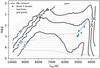 |
Fig. 5 EW contours (in mÅ) of blending lines across the Kiel diagram, i.e. Teff–log (𝑔), in solar metallicity and GIANO-B resolution (R = 50 000). The grey circles are the grid points used to calculate the contours, and the blue points indicate our Stock 2 sample. The isochrone used in Fig. 1 is plotted as a reference. |
4.2 Measurement of Ca II lines
The core emission of the Ca II H and K lines is commonly quantified through the  index:
 (3)
(3)
where  represent the integrated absolute flux (in the unit of erg s−1 cm−2) at the stellar surface for the bands located in the centres of the H and K line after excluding those emitted in the photosphere. The S -index, defined as the ratio of the normalised flux between the triangle windows at the centre of Ca II H&K lines and two windows on both sides of the lines (Wilson 1968), can also be used to quantify the Ca II H&K core emission. However, it contains a photospheric contribution at the line core and is also found to be sensitive to the colour of the star (see e.g. Figs. 1 and 2 in Noyes et al. 1984). Thus,
  can better represent the condition in the stellar chromosphere compared to S-index, and we limited ourselves to
  in the following analysis.
Our method of measuring the  index is described as follows. The photospheric flux at the centre of Ca II H&K are adopted from the synthetic spectra. As shown in Figs. 7 and 8, we first extracted high-resolution synthetic spectra with no chromo-spheric contribution from the PHOENIX database (Husser et al. 2013) using Starfish5, which were then broadened and resam-pled to match the spectral resolution of our sample. The observed spectra were then vertically scaled by fitting a spline function to a 60-pixel running median to the ratio between the observed and model flux in the wavelength range between 3921 and 3989 Å.
The strong and broad spectral lines and the core of Ca II H&K lines were masked out before the spline fitting. Finally,  were measured from the difference between the observed and synthetic spectra in the line cores of the K and H bands wherever there was an obvious difference between the observed and synthetic spectrum (the orange areas at the line centres in Figs. 7 and 8), from which the
  indices were then determined. This procedure is similar to the one adopted by Frasca et al. (2023) for measuring Ca II H&K fluxes for the members of ASCC123 observed with HARPS-N.
The final He 10 830 measurement results, including the EW, FWHM, line centre wavelength, and the blue-to-red ratio of the primary and secondary components, along with the  index measurement results, are summarised in Table 4. The EWs of the main He 10 830 feature exhibit a range from 84 to 471 mÅ, and their corresponding errors are approximately 10 mÅ, thanks to the high spectral resolution and high S/N. All of the He 10 830 features in our sample are in the form of absorption and can be easily seen in all the spectra (see Fig. 6).
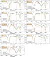 |
Fig. 6 Observed (blue; without telluric correction) and fitted spectra (orange) for our sample stars. The main and secondary components of He 10 830 are fitted as the green and red curve, respectively. |
 |
Fig. 7 Ca II H&K spectra for stars g1–g5, scaled to the PHOENIX scale. The vertical grey strips indicate the lines masked out before the spline fitting, and the orange shaded areas in the middle of the lines are used for measuring the |

5 Result and discussion
5.1 Two He components
The nine giants in our sample are separated into two groups: Stars g2, g5, and g10 have a relatively large EWs (i.e. greater than 350 mÅ), while others have EWs of around 100 mÅ.
The three stars with stronger He 10830 absorption also show a secondary absorption component around the wavelength λ = 10 829.088 Å (see their spectra in Fig. 6). The EW of the secondary He 10 830 component is around 5–10% of their main component.
The existence of the secondary component has been reported in the literature, though mainly for main sequence stars (see e.g. Takeda & Takada-Hidai 2011; Andretta et al. 2017). In Takeda & Takada-Hidai (2011) the second He 10 830 component is displayed (see their Fig. 2) but not measured because the 10 829.088 Å line is considerably weaker than the other two He lines. This component is called ‘the minor component’ in Andretta et al. (2017) for the X-ray dwarf stars. Its EW, if can be fitted independently, is around 15–25% of the main component, which is larger than the ratios we measured in our giant sample stars. Andretta et al. (2017) suggest that the ratio should be 1:8 (12.5%) in optically thin condition according to Russell-Saunders coupling, and different ratios refer to the different optical thicknesses of the He line components. Future observations of stars covering different evolutionary stages but similar stellar populations may shed light on the discrepancy between our results on giant stars and their results on dwarfs. For instance, understanding whether the possible difference in the chromosphere structure between dwarf and giant is the main factor affecting the strength ratio.
Measurement results of the sample stars.
5.2 He 10 830 line asymmetry
Given that the He 10 830 lines originate from the upper chromosphere of the stars, their line asymmetry provides insights into the local environment’s motion. In our sample stars, the He 10 830 line shapes do not exhibit any evidence of bulk motion in their upper chromosphere. The line centre wavelengths of both the main and the second components are corrected for the radial velocities of each star (adopted from the Table 2 of Alonso-Santiago et al. 2021). Following this correction, the centre wavelengths of the main components are closely aligned with their rest wavelengths. A minor redshift is detected, corresponding to a velocity of 0–9 km s−1. This subtle shift indicates the absence of significant systematic mass motions in the region where the He 10 830 line forms (i.e. in the upper chromosphere). According to the results presented in Table 4, the B/R ratio is found to be very close to 1 for both the main and second components of He 10 830. This result suggests that both components exhibit a high degree of symmetry.
An asymmetrical He 10830 absorption line is not always the case for giant stars. Dupree et al. (1992) studied the He 10 830 profile of a few field stars, including HD 6833, α Boo, and α Aqr, and found that their He 10 830 present a P Cygni profile, that is, an emission He line with absorption on the blueward side. They concluded that such a profile of HD 6833 indicates a very strong mass loss from the star, with a motion velocity of at least 90 km s−1, and the other stars show similar profiles.
Conversely, the symmetric He 10 830 profile exhibited by our sample stars, closely aligned with or around their rest wavelengths, suggests that the region where the line forms – the upper chromosphere – experiences negligible or small bulk motion. This is not surprising because our sample stars are very likely in the RC stage, which is less affected by mass loss (Girardi 1999). The stars in Dupree et al. (2009) are more active than our sample, since they are located higher on the RGB and stronger outflows are expected. We note, however, that a larger sample of stars with He 10 830 measurements is necessary to validate the slightly redshifted trend in our sample stars.
5.3 The EW(He)- relation
We observe a correlation between the strength of the main He 10830 component and the  index. As depicted in Fig. 9, stars exhibiting a less pronounced core emission in the Ca II H&K lines, denoted by
  , also display weaker helium absorption in their spectra. Conversely, the three stars characterised by larger EW and a secondary He component demonstrate stronger Ca II H&K core emission (
 ). This observation suggests a connection between stronger stellar activity and the enhanced strength of the He 10 830 feature.
A similar positive relation between the strength of He 10 830 and  was reported in Smith (2016) for the Galactic field dwarf and sub-dwarf stars. Their sample stars are predominantly population I, with a small number of population II dwarfs. For comparison, we overplot their results in Fig. 9 with grey dots and fit a linear line to show their relation with EW and the
  index. Stars in Smith (2016) with
  show a weak absorption of EW ~ 50 mÅ, whilst those with
  show EW ~ 200 mÅ.
Dwarf and sub-dwarf stars, as observed in Smith (2016), consistently exhibit smaller He 10 830 EW systematically compared to RC stars of Stock 2 studied in this work. This disparity primarily stems from differences in the surface helium abundance between dwarf and RC stars, under the assumption of similar initial metallicities and helium abundances. We delved into this aspect in our sample selection process, as detailed in Sect. 2, and illustrated in Fig. 2. Additionally, it is worth noting that variations in resolution and differences in measurement methods, such as how the continuum was determined, between the two studies, could also contribute to the observed disparity in EW.
The variation of the He 10 830 EW in the Stock 2 RC stars, together with the strong positive correlation between the He 10 830 EW and  shown in Fig. 9, suggests that the chromosphere structure affects the He 10 830 feature, and it needs to be checked before using He 10 830 to probe the stellar helium abundance. A possible approach to checking the chromosphere structure is observing Ca II H&K lines and He 10 830 simultaneously, then either comparing the He 10 830 with stars showing similar Ca II H&K core emission (Pasquini et al. 2011) or determining the chromosphere structure from Ca II H&K lines and fitting He 10 830 by varying the helium abundance (Dupree & Avrett 2013).
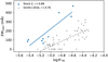 |
Fig. 9 EW(He) of the main He 10 830 component versus |

5.4 Comparison with previous He 10 830 measurements
Our EW measurement of the Stock 2 sample is compared with those obtained in previous studies, as illustrated in Fig. 10. The data from literature encompass field red giants sourced from Sanz-Forcada & Dupree (2008), Dupree et al. (2009), and Takeda & Takada-Hidai (2011), in addition to giants hailing from the globular cluster ω Cen (Dupree et al. 2011; Navarrete et al. 2015). It is worth noting that these stars either exhibit significant activity levels (in the case of stars from Sanz-Forcada & Dupree 2008) or are characterised by their metal-poor nature as globular cluster members. The He 10 830 strengths of the active giants in the literature are ~800 mÅ, while the other giants with lower [Fe/H] (dark colour in the figure) have a much weaker absorption, around 50 mÅ. The He 10 830 strength of the asymptotic giant branch stars is also ~50 mÅ, while that of the horizontal branch stars are stronger for higher Teff, as reported in Strader et al. (2015).
The strength of He 10 830 in our sample lies in between the very active giants and metal-poor giants from previous studies. The EW of stars with weaker He 10 830 absorption is slightly larger than the metal-poor giants, while the three giants with the largest EW have weaker features than the active giants. Since most of the giants from previous studies have a [Fe/H] lower than −1, the slightly larger EW of our sample may imply that the metal-rich stars have a slightly stronger He 10 830 than inactive metal-poor stars. Due to the difference in how the He 10 830 is measured in all these studies, a homogeneous measurement of He 10 830 using the same method with a larger sample with [Fe/H] from −1 to solar for both dwarfs and giants would yield a better conclusion on the possible metallicity effect.
5.5 Future applications
The method we developed in this study to measure the strength and profile of He 10 830 can be applied to other datasets. The high resolution of the GIANO-B spectrograph enables the log 𝑔f calibration for the blending lines, which quantifies the blending line EW, not only for the current dataset, but also for other stars across the HR diagram. The difference between the calibrated and original log 𝑔f values suggests that the line parameters in this wavelength are not accurate and need to be calibrated, or that other effects are playing a role in the formation of these lines. He 10 830 is well sampled in the observed spectra, which provides information on the profile of this feature. In a forthcoming paper we will apply this method to other open clusters observed in the SPA large programme. The method can also be applied to spectra at lower resolutions, such as those observed with the WIDE mode of the Warm INfrared Echelle spectrograph to Realize Extreme Dispersion and sensitivity (WINERED; R ≈ 28 000; Ikeda et al. 2022). The data from spectrographs that can cover Ca II H&K and He 10 830 simultaneously, for example X-shooter (Vernet et al. 2011), will also provide vital information on the behaviour of He 10 830. Such an observation is especially useful for globular cluster giants, whose helium abundances are expected to be varied. In short, we foresee the application of our method to the data obtained by various spectrographs across various types of stars in future works.
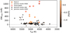 |
Fig. 10 EW(He) versus Teff for the Stock 2 stars with giants from previous studies. The EWs smaller than 0 indicate that the He 10 830 is in emission. |
6 Summary
In this paper, we have presented a pilot study of the helium content in the Stock 2 RC stars using the He 10 830 spectral line. Understanding stellar helium abundances is crucial for comprehending both stellar evolution and the chemical evolution of the Galaxy. Galactic open clusters, with their well-defined single stellar populations, provide an ideal setting for exploring the helium spectral line feature. We specifically chose RC stars for their constant surface helium abundance in a single stellar population, aiming to avoid potential intrinsic helium abundance dispersion induced by stellar evolution.
The He 10 830 profiles of our sample stars exhibit symmetric shapes and align with or are near their rest wavelengths, indicating the absence of significant bulk motion in the upper chromosphere of these stars. We removed the blending lines of Ca I, Fe I, Si I, Fe I, and Ti I in the He 10 830 region before measuring the helium line strength. Their abundances were determined from simultaneously observed optical high-resolution spectra, The oscillator strengths (log 𝑔f) of these lines were calibrated 'astronomically' during this process.
The final He 10 830 line strengths of these RC stars fall into two distinct categories. Three stars exhibit strong absorption, including a discernible secondary component related to the weaker line (at 10 829.09 Å) of the He 10 830 triplet, while the remaining stars display weaker absorption. We identify a correlation between the main component of the He 10 830 line strength and the Ca II  values. This result highlights the importance of accounting for stellar chromosphere structure when using the He 10 830 line as an abundance indicator.
The method developed in this study sheds light on the possibility of using the He 10 830 spectral line to probe stellar helium content when simultaneous observations of other chromospheric diagnostics are available. The results can be further compared to helium measurements from future asteroseismology missions such as the High-precision AsteroseismologY of DeNse stellar fields mission (HAYDN; Miglio et al. 2021). We plan to extend this approach to additional open clusters and field stars that span a broader range of Galactic regions and metallicities. This will allow us to gain a more comprehensive understanding of helium abundance variations across different stellar populations and their implications for stellar and Galactic evolution.
Acknowledgements
This study is supported by JSPS KAKENHI Grant-in-Aid 21J11301. X.F. thanks the support of the National Natural Science Foundation of China (NSFC) No. 12203100 and the China Manned Space Project with No. CMS-CSST-2021-A08. A.B. acknowledges funding from Mini-Grant INAF 2022 (High Resolution Observations of Open Clusters). A.F. acknowledges funding from the Large-Grant INAF YODA (YSOs Outflow, Disks and Accretion). The data of this study is based on observations made with the Italian Telescopio Nazionale Galileo (TNG) operated on the island of La Palma by the Fundación Galileo Galilei of the INAF (Istituto Nazionale di Astrofisica) at the Spanish Observatorio del Roque de los Muchachos of the Instituto de Astrofisica de Canarias. This research used the facilities of the Italian centre for Astronomical Archive (IA2) operated by INAF at the Astronomical Observatory of Trieste. This work has made use of the VALD database, operated at Uppsala University, the Institute of Astronomy RAS in Moscow, and the University of Vienna.
References
- Alonso-Santiago, J., Frasca, A., Catanzaro, G., et al. 2021, A&A, 656, A149 [NASA ADS] [CrossRef] [EDP Sciences] [Google Scholar]
- Andreasen, D. T., Sousa, S. G., Delgado Mena, E., et al. 2016, A&A, 585, A143 [NASA ADS] [CrossRef] [EDP Sciences] [Google Scholar]
- Andretta, V., & Jones, H. P. 1997, ApJ, 489, 375 [NASA ADS] [CrossRef] [Google Scholar]
- Andretta, V., Giampapa, M. S., Covino, E., Reiners, A., & Beeck, B. 2017, ApJ, 839, 97 [Google Scholar]
- Athay, R. G., & Menzel, D. H. 1956, ApJ, 123, 285 [NASA ADS] [CrossRef] [Google Scholar]
- Avrett, E. H., Fontenla, J. M., & Loeser, R. 1994, in Infrared Solar Physics, eds. D. M. Rabin, J. T. Jefferies, & C. Lindsey (Dordrecht: Kluwer Academic Publishers), IAU Symp., 154, 35 [NASA ADS] [Google Scholar]
- Bastian, N., & Lardo, C. 2018, ARA&A, 56, 83 [Google Scholar]
- Bragaglia, A., Carretta, E., Gratton, R., et al. 2010, A&A, 519, A60 [NASA ADS] [CrossRef] [EDP Sciences] [Google Scholar]
- Bressan, A., Marigo, P., Girardi, L., et al. 2012, MNRAS, 427, 127 [NASA ADS] [CrossRef] [Google Scholar]
- Cantat-Gaudin, T., Jordi, C., Vallenari, A., et al. 2018, A&A, 618, A93 [NASA ADS] [CrossRef] [EDP Sciences] [Google Scholar]
- Casali, G., Magrini, L., Frasca, A., et al. 2020, A&A, 643, A12 [NASA ADS] [CrossRef] [EDP Sciences] [Google Scholar]
- Castelli, F., & Kurucz, R. L. 2003, in Modelling of Stellar Atmospheres, eds. N. Piskunov, W. W. Weiss, & D. F. Gray, 210, A20 [Google Scholar]
- Chen, Y., Girardi, L., Fu, X., et al. 2019, A&A, 632, A105 [EDP Sciences] [Google Scholar]
- Claudi, R., Benatti, S., Carleo, I., et al. 2017, Eur. Phys. J. Plus, 132, 364 [NASA ADS] [CrossRef] [Google Scholar]
- Cosentino, R., Lovis, C., Pepe, F., et al. 2012, SPIE Conf. Ser., 8446, 84461V [Google Scholar]
- Cui, X.-Q., Zhao, Y.-H., Chu, Y.-Q., et al. 2012, Res. Astron. Astrophys., 12, 1197 [Google Scholar]
- Dib, S., Schmeja, S., & Parker, R. J. 2018, MNRAS, 473, 849 [Google Scholar]
- Dupree, A. K., & Avrett, E. H. 2013, ApJ, 773, L28 [Google Scholar]
- Dupree, A. K., Sasselov, D. D., & Lester, J. B. 1992, ApJ, 387, L85 [CrossRef] [Google Scholar]
- Dupree, A. K., Smith, G. H., & Strader, J. 2009, AJ, 138, 1485 [NASA ADS] [CrossRef] [Google Scholar]
- Dupree, A. K., Strader, J., & Smith, G. H. 2011, ApJ, 728, 155 [NASA ADS] [CrossRef] [Google Scholar]
- Frasca, A., Alonso-Santiago, J., Catanzaro, G., & Bragaglia, A. 2023, MNRAS, 522, 4894 [NASA ADS] [CrossRef] [Google Scholar]
- Fu, X., Bressan, A., Molaro, P., & Marigo, P. 2015, MNRAS, 452, 3256 [CrossRef] [Google Scholar]
- Girardi, L. 1999, MNRAS, 308, 818 [CrossRef] [Google Scholar]
- Gratton, R., Bragaglia, A., Carretta, E., et al. 2019, A&A Rev., 27, 8 [NASA ADS] [CrossRef] [Google Scholar]
- Gullikson, K., Dodson-Robinson, S., & Kraus, A. 2014, AJ, 148, 53 [NASA ADS] [CrossRef] [Google Scholar]
- Hirayama, T. 1971, Sol. Phys., 17, 50 [NASA ADS] [CrossRef] [Google Scholar]
- Holtzman, J. A., Hasselquist, S., Shetrone, M., et al. 2018, AJ, 156, 125 [Google Scholar]
- Husser, T. O., Wende-von Berg, S., Dreizler, S., et al. 2013, A&A, 553, A6 [NASA ADS] [CrossRef] [EDP Sciences] [Google Scholar]
- Ikeda, Y., Kondo, S., Otsubo, S., et al. 2022, PASP, 134, 015004 [CrossRef] [Google Scholar]
- Jian, M., Satheesh, P., Krishna, K., et al. 2023, https://doi.org/10.5281/zenodo.7666783 [Google Scholar]
- Kondo, S., Fukue, K., Matsunaga, N., et al. 2019, ApJ, 875, 129 [NASA ADS] [CrossRef] [Google Scholar]
- Lee, Y.-W., Joo, S.-J., Han, S.-I., et al. 2005, ApJ, 621, L57 [NASA ADS] [CrossRef] [Google Scholar]
- Miglio, A., Girardi, L., Grundahl, F., et al. 2021, Exp. Astron., 51, 963 [NASA ADS] [CrossRef] [Google Scholar]
- Navarrete, C., Chanamé, J., Ramírez, I., et al. 2015, ApJ, 808, 103 [NASA ADS] [CrossRef] [Google Scholar]
- Noyes, R. W., Hartmann, L. W., Baliunas, S. L., Duncan, D. K., & Vaughan, A. H. 1984, ApJ, 279, 763 [Google Scholar]
- Obrien, J., George T., & Lambert, D. L. 1986, ApJS, 62, 899 [NASA ADS] [CrossRef] [Google Scholar]
- Oliva, E., Origlia, L., Baffa, C., et al. 2006, SPIE Conf. Ser., 6269, 626919 [Google Scholar]
- Origlia, L., Dalessandro, E., Sanna, N., et al. 2019, A&A, 629, A117 [NASA ADS] [CrossRef] [EDP Sciences] [Google Scholar]
- Pasquini, L., Mauas, P., Käufl, H. U., & Cacciari, C. 2011, A&A, 531, A35 [NASA ADS] [CrossRef] [EDP Sciences] [Google Scholar]
- Piotto, G., Bedin, L. R., Anderson, J., et al. 2007, ApJ, 661, L53 [NASA ADS] [CrossRef] [Google Scholar]
- Rainer, M., Harutyunyan, A., Carleo, I., et al. 2018, SPIE Conf. Ser., 10702, 1070266 [Google Scholar]
- Reddy, A. B. S., & Lambert, D. L. 2019, MNRAS, 485, 3623 [NASA ADS] [CrossRef] [Google Scholar]
- Ryabchikova, T., Piskunov, N., Kurucz, R. L., et al. 2015, Phys. Scr, 90, 054005 [Google Scholar]
- Sanz-Forcada, J., & Dupree, A. K. 2008, A&A, 488, 715 [NASA ADS] [CrossRef] [EDP Sciences] [Google Scholar]
- Smith, M. A. 1983, AJ, 88, 1031 [NASA ADS] [CrossRef] [Google Scholar]
- Smith, G. H. 2016, PASA, 33, e057 [CrossRef] [Google Scholar]
- Smith, G. H., Dupree, A. K., & Strader, J. 2004, PASP, 116, 819 [NASA ADS] [CrossRef] [Google Scholar]
- Smith, G. H., Dupree, A. K., & Strader, J. 2012, PASP, 124, 1252 [NASA ADS] [CrossRef] [Google Scholar]
- Sneden, C., Bean, J., Ivans, I., Lucatello, S., & Sobeck, J. 2012, MOOG: LTE line analysis and spectrum synthesis, Astrophysics Source Code Library [record ascl:1202.009] [Google Scholar]
- Stock, J. 1956, ApJ, 123, 258 [NASA ADS] [CrossRef] [Google Scholar]
- Strader, J., Dupree, A. K., & Smith, G. H. 2015, ApJ, 808, 124 [NASA ADS] [CrossRef] [Google Scholar]
- Takeda, Y. 1995, PASJ, 47, 287 [NASA ADS] [Google Scholar]
- Takeda, Y., & Takada-Hidai, M. 2011, PASJ, 63, 547 [NASA ADS] [Google Scholar]
- Vaughan, J., Arthur H., & Zirin, H. 1968, ApJ, 152, 123 [NASA ADS] [CrossRef] [Google Scholar]
- Vernet, J., Dekker, H., D’Odorico, S., et al. 2011, A&A, 536, A105 [NASA ADS] [CrossRef] [EDP Sciences] [Google Scholar]
- Villanova, S., Piotto, G., & Gratton, R. G. 2009, A&A, 499, 755 [NASA ADS] [CrossRef] [EDP Sciences] [Google Scholar]
- Wilson, O. C. 1968, ApJ, 153, 221 [Google Scholar]
- Ye, X., Zhao, J., Liu, J., et al. 2021, AJ, 161, 8 [NASA ADS] [CrossRef] [Google Scholar]
- Zarro, D. M., & Zirin, H. 1986, ApJ, 304, 365 [NASA ADS] [CrossRef] [Google Scholar]
- Zhang, R., Lucatello, S., Bragaglia, A., et al. 2021, A&A, 654, A77 [NASA ADS] [CrossRef] [EDP Sciences] [Google Scholar]
- Zirin, H. 1975, ApJ, 199, L63 [NASA ADS] [CrossRef] [Google Scholar]
- Zirin, H. 1976, ApJ, 208, 414 [NASA ADS] [CrossRef] [Google Scholar]
- Zirin, H. 1982, ApJ, 260, 655 [NASA ADS] [CrossRef] [Google Scholar]
Obtained from the CMD 3.7 input form http://stev.oapd.inaf.it/cgi-bin/cmd
They are integrated into the python wrapper pymoog (Jian et al. 2023).
![$V\left( {x;{x_0},a,\gamma ,\sigma } \right) = \int_{ - \infty }^\infty {{1 \over {\sigma \sqrt {2\pi } }}} {{\rm{e}}^{ - {{{{x'}^2}} \over {2{\sigma ^2}}}}}{{a\gamma } \over {\pi \left[ {{{\left( {x - {x_0} - {x^\prime }} \right)}^2}} \right] + {\gamma ^2}}}{\rm{d}}{x^\prime }$](/articles/aa/full_html/2024/07/aa49476-24/aa49476-24-eq28.png)
All Tables
All Figures
|
Fig. 1 CMD in Gaia DR2 photometry bands of Stock 2 member stars (grey) from Cantat-Gaudin et al. (2018), with the sample stars in this study marked with orange circles. The PARSEC isochrone with an age of 450 Myr, [M/H] = −0.07 and an extinction of AV = 0.84 is overplotted in blue. |
| In the text | |
|
Fig. 2 He mass fraction (Y) on the stellar surface as a function of surface gravity, log (𝑔), for the Stock 2 isochrone. The initial He mass fraction of this isochrone is Y0 = 0.2712. The locations of the MSTO, RGB onset, and RC phase are highlighted. |
| In the text | |
|
Fig. 3 Observed (blue step line; with telluric correction) and the synthetic spectra before (orange) and after (green) their log 𝑔f values are calibrated (without the He 10 830) for star g1. Vertical dashed red lines indicate the position of the He 10 830 triplet, and the black arrows indicate the position of blending lines with log 𝑔f values calibrated (see Sect. 3). The spectra of the other eight target stars are plotted in grey as a reference. |
| In the text | |
|
Fig. 4 Measured stellar parameters. Left panel: measured ξ from MPFIT versus log (𝑔) for the Stock 2 stars, along with the relation reported in Holtzman et al. (2018). Right panel: [Fe/H] values determined from GIANO-B spectra versus those from HARPS-N (Alonso-Santiago et al. 2021), with the histogram of Δ[Fe/H] = [Fe/H]GIANO-B ~ [Fe/H]harps-n in the upper-left corner. |
| In the text | |
|
Fig. 5 EW contours (in mÅ) of blending lines across the Kiel diagram, i.e. Teff–log (𝑔), in solar metallicity and GIANO-B resolution (R = 50 000). The grey circles are the grid points used to calculate the contours, and the blue points indicate our Stock 2 sample. The isochrone used in Fig. 1 is plotted as a reference. |
| In the text | |
|
Fig. 6 Observed (blue; without telluric correction) and fitted spectra (orange) for our sample stars. The main and secondary components of He 10 830 are fitted as the green and red curve, respectively. |
| In the text | |
|
Fig. 7 Ca II H&K spectra for stars g1–g5, scaled to the PHOENIX scale. The vertical grey strips indicate the lines masked out before the spline fitting, and the orange shaded areas in the middle of the lines are used for measuring the |
| In the text | |
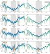 |
Fig. 8 Same as Fig. 7, but for stars g6, g7, g9, and g10. |
| In the text | |
|
Fig. 9 EW(He) of the main He 10 830 component versus |
| In the text | |
|
Fig. 10 EW(He) versus Teff for the Stock 2 stars with giants from previous studies. The EWs smaller than 0 indicate that the He 10 830 is in emission. |
| In the text | |
Current usage metrics show cumulative count of Article Views (full-text article views including HTML views, PDF and ePub downloads, according to the available data) and Abstracts Views on Vision4Press platform.
Data correspond to usage on the plateform after 2015. The current usage metrics is available 48-96 hours after online publication and is updated daily on week days.
Initial download of the metrics may take a while.