| Issue |
A&A
Volume 689, September 2024
|
|
|---|---|---|
| Article Number | A204 | |
| Number of page(s) | 25 | |
| Section | Extragalactic astronomy | |
| DOI | https://doi.org/10.1051/0004-6361/202449470 | |
| Published online | 13 September 2024 | |
Demographics of tidal disruption events with L-Galaxies
I. Volumetric TDE rates and the abundance of nuclear star clusters
1
Donostia International Physics Center, Paseo Manuel de Lardizabal 4, 20118
Donostia-San Sebastián, Spain
2
University of the Basque Country UPV/EHU, Department of Theoretical Physics, Bilbao, 48080
Spain
3
IKERBASQUE, Basque Foundation for Science, 48013
Bilbao, Spain
4
Dipartimento di Fisica ‘G. Occhialini’, Universitá degli Studi di Milano-Bicocca, Piazza della Scienza 3, 20216
Milano, Italy
5
INFN, Sezione di Milano-Bicocca Piazza della Scienza 3, 20126
Milano, Italy
6
INAF – Osservatorio Astronomico di Brera, Via Brera 20, 20121
Milano, Italy
7
Max-Planck-Institut für Astronomie, Königstuhl 17, 69117
Heidelberg, Germany
8
Institute of Astronomy, Pontificia Universidad Católica de Chile, Avenida Vicuña Mackena 4690, Santiago, Chile
9
Universität Heidelberg, Seminarstrasse 2, 69117
Heidelberg, Germany
10
Department of Astronomy, MongManWai Building, Tsinghua University, Beijing, 100084
China
Received:
2
February
2024
Accepted:
11
June
2024
Stars can be ripped apart by tidal forces in the vicinity of a massive black hole (MBH), causing luminous flares known as tidal disruption events (TDEs). These events could be contributing to the mass growth of intermediate-mass MBHs. New samples from transient surveys can provide useful information on this unexplored growth channel. This work aims to study the demographics of TDEs by modeling the coevolution of MBHs and their galactic environments in a cosmological framework. We use the semianalytic galaxy formation model L-Galaxies BH, which follows the evolution of galaxies as well as of MBHs, including multiple scenarios for MBH seeds and growth, spin evolution, and binary MBH dynamics. We associated time-dependent TDE rates with each MBH depending on the stellar environment, following the solutions to the 1D Fokker Planck equation solved with PHASEFLOW. Our model produces volumetric rates that are in agreement with the latest optical and previous X-ray samples. This agreement requires a high occupation fraction of nuclear star clusters with MBHs since these star reservoirs host the majority of TDEs at all mass regimes. We predict that TDE rates are an increasing function of MBH mass up to ∼105.5 M⊙, beyond which the distribution flattens and eventually drops for > 107 M⊙. In general, volumetric rates are predicted to be redshift independent at z < 1. We discuss how the spin distribution of MBHs around the event horizon suppression can be constrained via TDE rates and the average contribution of TDEs to the MBH growth. In our work, the majority of low-mass galaxies host nuclear star clusters that have their loss-cone depleted by z = 0, explaining why TDEs are rare in these systems. This highlights how essential time-dependent TDE rates are for any model to be in good agreement with observations at all mass regimes.
Key words: galaxies: nuclei / galaxies: statistics
© The Authors 2024
 Open Access article, published by EDP Sciences, under the terms of the Creative Commons Attribution License (https://creativecommons.org/licenses/by/4.0), which permits unrestricted use, distribution, and reproduction in any medium, provided the original work is properly cited.
This article is published in open access under the Subscribe to Open model. Subscribe to A&A to support open access publication.
1. Introduction
A tidal disruption event (TDE) occurs when a star wanders too close to a massive1 black hole (MBH) so that the MBH gravitational pull overcomes the star’s self-gravity. As a result, the star becomes “spaghettified”, and a part of it settles into a disk-like configuration, producing a distinct, multiwavelength electromagnetic flare. Tidal disruption events can outshine their host galaxies, with luminosities of 1042 − 1045 erg s−1 that decline over timescales of weeks to years. Most TDEs can be identified by the characteristic post-peak decrease of their accretion rate, which drops for most of the events as ∝t−5/3, as predicted by the standard fallback theory (Rees 1988; Phinney et al. 1989).
The first observations of TDE-like transients, initially in the X-ray (e.g. Bade et al. 1996; Komossa & Bade 1999; Esquej et al. 2008) and then in the optical/UV sky (Gezari et al. 2006, 2008; van Velzen et al. 2011), sparked interest in their overall rate per galaxy (Magorrian & Tremaine 1999; Syer & Ulmer 1999; Wang & Merritt 2004). Such interest has increased at the present date, as the number of observed TDEs has grown more quickly than ever (approximately 100 TDE candidates have now been identified), mainly owing to the advent of wide-field transient optical surveys, such as Pan-STARRS1 (Chornock et al. 2014), the Palomar Transient Factory (PTF; e.g. Cenko et al. 2012; Arcavi et al. 2014), the ongoing Zwicky Transient Facility (ZTF; e.g. Lin et al. 2022; Hammerstein et al. 2023; Yao et al. 2023), and ASAS-SN (e.g., Krolik et al. 2016; Hinkle et al. 2021; Liu et al. 2023). In the X-rays, eROSITA has already provided a sample of candidates (Sazonov et al. 2021), adding to previously compiled inventories from Swift, XMM-Newton, and Chandra (Kawamuro et al. 2016; Auchettl et al. 2017; Goldtooth et al. 2023). Finally, individual dust-shrouded TDE candidates have been detected in the mid-infrared (Mattila et al. 2018; Kool et al. 2020; Wang et al. 2022; Panagiotou et al. 2023), and a recent analysis of NEOWISE data has yielded the first sample at this wavelength (Masterson et al. 2024).
The collection of these growing samples has allowed the TDE rates to be assessed. In particular, the works of van Velzen (2018), Lin et al. (2022), and Yao et al. (2023) have used a relatively wide sample of observed TDEs to infer an overall volumetric rate of ∼10−7 − 10−6 Mpc−3 yr−1
 , with Lb as the peak luminosity within the band of a given survey, corresponding to a number of TDEs per galaxy on the order of 10−5 − 10−4 yr−1. Although these results necessarily depend on the shape of the TDE luminosity function, which remains uncertain, the obtained rates are in decent agreement with (although somewhat lower than) the TDE rates predicted by theoretical and numerical studies (Syer & Ulmer 1999; Magorrian & Tremaine 1999; Donley et al. 2002; Wang & Merritt 2004; Esquej et al. 2008; Merritt 2009; Brockamp et al. 2011; Stone & Metzger 2016; Pfister et al. 2021; Broggi et al. 2022). Nevertheless, both observational and theoretical estimates suffer from several limitations. On one side, the available sample of observed TDEs is still relatively small. However, for simplicity, theoretical models typically neglect important ingredients such as the time evolution of TDE rates under the evolution of the host galaxy. Most models are also affected by our poor knowledge of the MBH mass function at low masses (≲107 M⊙, see Shankar et al. 2013; Greene et al. 2020) and the occupation fraction of nuclear star clusters (NSCs; see recent studies Hoyer et al. 2023; Ashok et al. 2023; Hoyer et al. 2024).
Still, currently available samples have allowed statistical studies on the host galaxies of observed TDEs to be performed (see French et al. 2020b for a review). In particular, ZTF observations have shed light on the fact that TDEs are overrepresented in ultra-luminous infrared galaxies (ULIRGs; Tadhunter et al. 2017; Reynolds et al. 2022) as well as in the rarer post-starburst (“green-valley”) galaxies (Hammerstein et al. 2021, 2023) and, in particular, in quiescent Balmer-strong (E+A) galaxies (Arcavi et al. 2014; French et al. 2016; Law-Smith et al. 2017; Graur et al. 2018; Dodd et al. 2021). The stellar mass distribution of TDE hosts is relatively flat compared to the stellar mass function, and it is concentrated in the dwarf-to-massive transition regime, ∼109 − 1011 M⊙ (Wevers et al. 2019). Interestingly, the occupation fraction of NSCs peaks in the same mass range (e.g. Sánchez-Janssen et al. 2019; Hoyer et al. 2021). That being said, MBHs and NSCs have frequently been related in many works (Antonini et al. 2015; Naiman et al. 2015; Trani et al. 2018; Askar et al. 2022; Atallah et al. 2023; Lee et al. 2023; Tremmel et al. 2024), yet the exact nature of their connection remains unknown. What seems to be evident from theoretical studies (Merritt 2009; Stone & Metzger 2016; Pfister et al. 2020) is that the presence of an NSC, the densest stellar system possible in the Universe (Neumayer et al. 2020), may enhance the rate of TDEs on the central MBH. Therefore, the majority of TDEs are expected to be related to intermediate-mass black holes (typically defined as 102.5 − 106 M⊙) in the center of NSCs. At the same time, the very existence of MBHs below 105 M⊙ is being challenged by the tentative and scarce observational evidence, especially toward the low end of the mass range (Mezcua 2017, but see recent robust evidence for an intermediate-mass black hole in Omega Centauri Häberle et al. 2024).
At this intermediate MBH mass scale, the majority (> 90%) of black holes are believed to be inactive (Greene et al. 2020; Mezcua & Domínguez Sánchez 2024), making samples inferred from observations of active galactic nuclei (AGN) incomplete. Also, mass measurements through spectral information become troublesome at low masses (Kormendy & Ho 2013). In fact, beyond the local Universe, where accurate dynamical measurements of MBH mass can be made, TDE observations serve as the only direct detection method of the dormant MBH population, as opposed to the indirect method of detecting relic AGN activity.
Finally, TDEs offer a viable channel of black hole growth (Hills 1975) that could in principle be dominant for MBHs that do not grow efficiently through gas accretion. After the first observations, the TDE growth channel was revisited (Magorrian & Tremaine 1999), with Milosavljević et al. (2006) proposing that low-mass MBHs (< 2 × 10⁶ M⊙) may acquire the majority of their mass through TDEs. Furthermore, Alexander & Bar-Or (2017) used this channel to set a lower limit on the masses of MBHs that can exist in the local Universe since all MBH seeds should grow either through gas or TDEs. The initial growth through TDEs has also been studied within zoom-in cosmological simulations (Pfister et al. 2021; Lee et al. 2023), and recently, high-resolution simulations have achieved growing a black hole seed by a factor of more than 20 within 1 Gyr (Rizzuto et al. 2023). Yet the argument of effective TDE growth has been questioned for low-mass galaxies since NSCs, which contribute mainly to the TDE rates, are not dense enough to fuel black hole growth by runaway tidal capture of stars (Miller & Davies 2012; Stone et al. 2017), a physical process that is more efficient at growing an intermediate-mass MBH in globular clusters (Portegies Zwart & McMillan 2002; Arca-Sedda 2016) and hierarchically merging star clusters (see recent advancements in e.g. Rantala et al. 2024). Nevertheless, a statistical study on the frequency of TDEs across a realistic population of stellar environments and the role of stellar accretion in the growth of MBHs has not been performed so far.
In this paper, we set the foundation to address many of the aforementioned theoretical uncertainties by combining, for the first time, a semianalytic model of galaxy and black hole evolution in a wide range of stellar environments with time-dependent TDE rates provided by a fast 1D-Fokker Planck solver. The paper is structured as follows: In Sect. 2, we describe our method for coupling the physics of TDEs in a given local environment with a variety of stellar environments. In Sect. 3, we describe our most important findings and compare our TDE rate predictions with new constraints. In particular, we focus on the cosmological evolution of TDE rates and the contribution from active MBHs. In Sect. 4, we complement our analysis by addressing the impact of the parameter choice and discussing the implications for the occupation fraction of NSCs, the MBH spin model, and MBH growth. In Sect. 5, we discuss some caveats and subjects that we aim to investigate explicitly in the future. Finally, we summarize the key aspects of our work in Sect. 6. Throughout the paper, we adopt a Lambda cold dark matter (ΛCDM) cosmology with parameters Ωm = 0.315, ΩΛ = 0.685, Ωb = 0.0493, σ8 = 0.826, and H0 = 67.4 km s−1 Mpc−1 (Planck Collaboration VI 2020).
2. Model description
In this work, we combined the semianalytical model of galaxy formation L-Galaxies with the 1D Fokker-Planck solver PHASEFLOW to estimate the time evolution of TDE rates and compared it with observations. In particular, we used a version of L-Galaxies, dubbed L-Galaxies BH throughout this work, which was developed to study a wide variety of physical processes that drive the evolution of the MBH population and its coevolution with galaxies. In this section, we first describe the L-Galaxies models and the additional physics included to model the TDE statistics. We then describe PHASEFLOW and how it is linked to L-Galaxies BH to assign TDE rates to MBHs.
2.1. The L-Galaxies semianalytic models: Dark matter merger trees and baryonic physics
The L-Galaxies semianalytic model is a well-tested model that tracks the cosmological evolution of the baryonic component of the Universe on top of dark matter merger trees (Croton et al. 2006; Guo et al. 2011; Henriques et al. 2015, 2020). It has been developed on and is mainly being applied to the dark matter merger trees of the Millennium-I (MS, Springel et al. 2005) and Millennium-II (MSII, Boylan-Kolchin et al. 2009) cosmological N-body simulations. In this work, we use the merger trees of the MSII which offer a higher mass resolution compared to the MS simulation. Specifically, the MSII has a dark matter particle resolution of 6.89 × 10⁶ h−1 M⊙ in a box size of 100 h−1 Mpc, enabling a good tracing of the cosmological evolution of halos where MBHs of 104 − 108 M⊙ are placed. Originally, the MSII was run by using the WMAP1 and 2dFGRS “concordance” ΛCDM framework (Spergel et al. 2003). However, the version of L-Galaxies used here applies the Angulo & White (2010) methodology to re-scale it to the cosmology of Planck 2018 data release (Planck Collaboration VI 2020). This re-scaling modifies by a factor of 0.96 and 1.12 the MSII box size and particle mass, respectively.
Regarding the baryonic component, the current paradigm of galaxy evolution assumes that, as soon as a dark matter halo collapses, an amount of baryons, equal to the baryon fraction multiplied by the halo mass, also collapses within it (White & Frenk 1991). During this process, the infalling baryons are heated up and distributed inside the dark matter halo in the form of a diffuse, spherical, and quasi-static hot gas atmosphere. With time, this gas is allowed to cool down and migrate toward the center of the halo at a rate that depends on redshift and halo mass (White & Rees 1978; Sutherland & Dopita 1993). Due to angular momentum conservation, the cooled gas settles in a disk-like structure characterized by a radially exponential distribution. Once the disk becomes massive enough, star formation is triggered giving rise to a stellar component distributed in a disk with specific angular momentum inherited from the cold gas (Croton et al. 2006). Right after any star formation event, massive and short-lived stars explode polluting the interstellar medium and injecting energy in their environment, which can warm up and/or eject part of the cold gas of the disk. As a consequence of the ongoing stellar disk growth, some galaxies are prone to become unstable, with the subsequent disk instabilities leading to the formation of a stellar bulge component (Efstathiou et al. 1982). Besides supernova explosions, L-Galaxies assumes that MBHs in the center of the galaxy can prevent the gas from cooling in massive galaxies by injecting kinetic energy into the surrounding medium via quiescent gas accretion directly from the hot gas component (dubbed as “radio mode” accretion, see Croton et al. 2006), thus hampering the supply of cold gas to a galaxy’s disk. On top of secular processes, L-Galaxies models the interactions between galaxies, occurring after a given time of the fusion of their parent DM halos. Such interactions include major and minor galaxy mergers and alter the structure of the remnant galaxy by triggering bursts of star formation and leading to the formation of a stellar bulge or pure elliptical structure. Finally, L-Galaxies also takes into account environmental processes such as ram pressure stripping or galaxy disruptions in its galaxy formation paradigm (Henriques et al. 2015).
To improve the time resolution offered by the outputs of the MSII simulation, L-Galaxies does an internal time interpolation between two consecutive snapshots, with the time resolution being dtstep ∼ 5 − 20 Myr, depending on redshift.
2.1.1. Massive black holes in L-Galaxies
The version of L-Galaxies BH used in this work, L-Galaxies, is based on the one presented in Henriques et al. (2015) with the modifications included in Izquierdo-Villalba et al. (2019, 2020, 2022) and Spinoso et al. (2023) to incorporate detailed massive black hole physics.
In brief, with respect to the model presented in Henriques et al. (2015), this new version adds a detailed model for the assembly (mass and spin) of nuclear MBHs, the dynamical evolution of MBH binaries, and the production of wandering MBHs (see Izquierdo-Villalba et al. 2020, 2022). Concerning the genesis of the first MBHs, L-Galaxies BH models the spatial variations of the intergalactic metallicity and the Lyman-Werner background2 produced by star formation events to account for the formation of heavy (i.e., Mseed ∼ 105 M⊙) and intermediate-mass (Mseed ∼ 103 − 104 M⊙) MBH seeds, respectively via the collapse of pristine massive gas clouds and runaway stellar mergers within dense high-redshift3 NSCs. The formation of light seeds (Mseed ∼ 102 M⊙) after the explosion of the first metal-free stars (PopIII) is accounted for by grafting/inheriting the evolved counterparts of light-seed modeled self-consistently by the GametQSO/dust model (see e.g. Valiante et al. 2016). We note that concerning the black hole seeding model presented in Spinoso et al. (2023), we adopt a slightly higher amplitude of the “grafting probability”, setting the parameter Gp = 0.25 (see Spinoso et al. 2023, for the definition of this parameter). This choice is motivated by the normalization of the z = 0 black hole mass function in the current work.
Once the first MBH seeds are formed, galaxy mergers and disk instabilities funnel new gas to the galactic nuclei, making it available for the growth of nuclear MBHs. The gas reaching the center is progressively consumed by the MBH first in an Eddington limited phase, followed by a sub-Eddington one (Bonoli et al. 2009; Izquierdo-Villalba et al. 2020). Episodes of gas accretion, on top of triggering BH growth, also modify its spin (Izquierdo-Villalba et al. 2020). The dynamical evolution of massive black hole binaries in a post-merger galaxy is two-fold (Begelman et al. 1980). During the pairing phase, the MBH(s) from the satellite galaxy migrate toward the galactic center via dynamical friction (following Binney & Tremaine 1987), forming a hard binary upon arrival at the nucleus. Then the hardening phase, where interactions with a circumbinary disc (gas-torque model by Dotti et al. 2015 and preferential growth as in Duffell et al. 2020) or the surrounding stars (following the model by Quinlan & Hernquist 1997; Sesana & Khan 2015) assist the gravitational-wave-driven evolution, along potential triplet interactions in the cases that a third MBHs comes in during the inspiral (modeled based on the results of Bonetti et al. 2018). The latter, along with gravitational recoil after merging of MBHs (as described in Lousto et al. 2012), can result in wandering MBHs. While L-Galaxies BH can track the evolution of wandering MBHs, we did not include that in this work for simplicity (see the discussion on TDEs from wandering MBHs in Sect. 5).
As an example of the capability of L-Galaxies BH to produce a realistic population of MBHs, in Fig. 1 we show the MBH mass function ϕ(M•), where M• is the black hole mass (throughout this work), and the MBH median spin distribution  at z = 0 and z = 5.5 for the version of L-Galaxies BH adopted in the current work. We compare our results with available data. Regarding the black hole mass function, as noted by Shankar et al. (2019), all observationally derived values seem to converge at the high mass-end (M• > 107.5 M⊙, Merloni & Heinz 2008; Cao 2010; Gallo & Sesana 2019; Shankar et al. 2009, 2013; Mutlu-Pakdil et al. 2016; Vika et al. 2009; Aversa et al. 2015). However, constraints in the intermediate-mass range M• ∼ 105 − 106 M⊙ are much less stringent. L-Galaxies BH agrees with the most optimistic estimates from Shankar et al. (2009) and over-estimates with respect to all other available constraints. Regarding the spin distribution, the model agrees with the constraints from Reynolds (2021) at high masses, yet it predicts high-to-maximal spin for MBHs in the intermediate mass range, where there are no observational constraints. TDEs can potentially offer as a new probe for both the MBH mass and spin distribution in this range (see discussion in Sect. 4.3).
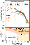 |
Fig. 1. Massive black hole mass function (top) and median spin for X-ray bright MBHs (bottom) as a function of the MBH mass M• predicted by the L-Galaxies BH model used in this work. Data are shown for z = 0 (red solid line) and z = 5.5 (yellow dashed line), with shaded areas in the bottom panel referring to the 1σ dispersion at a given mass range. In the top panel, the gray dashed line corresponds to the MBH mass function value equal to 1 dex−1 per MSII simulation volume. The results are compared with observational data at z = 0; MH08, Vika09, Sh09, Cao10, Sh13, Arvs15, GS19, and MuPa16 refer to the model-dependent constraints on the MBH mass function derived respectively by Merloni & Heinz (2008), Cao (2010), Gallo & Sesana (2019), Shankar et al. (2009, 2013), Mutlu-Pakdil et al. (2016), Vika et al. (2009), Aversa et al. (2015). For spin constraints, we display the upper and lower limits from X-ray reflection spectroscopy (Reynolds 2021). For a closer comparison to observational results, the average spin values shown here are for MBHs with a predicted hard X-ray luminosity of log LHX > 40 erg s−1. |
2.1.2. The stellar environment of massive black holes
As mentioned above, the novelty of this work is the inclusion of TDEs within a full galaxy evolution context. To encompass this ambitious task it is necessary to model the stellar environment in which MBHs are embedded, on top of their formation and evolution. In this section, we describe how disks, bulges, and NSCs are included in L-Galaxies BH. Together with black hole masses, the properties of the nuclear stellar environment will be the input for predicting time-evolving TDE rates with PHASEFLOW.
2.1.3. Bulge and disk profiles in L-Galaxies
Bulges in L-Galaxies BH grow after galaxy interactions (major and minor mergers) and disk instabilities occurring in massive stellar disks. The specific properties of these events fully determine the final mass and extension (i.e., effective size) of the bulge. We stress that the scale length for disks Reff, d and the effective size of bulges Reff, b (equivalent to the scale radius of a Sérsic profile) are computed self-consistently inside L-Galaxies BH by tracing the spin evolution of the galaxy components and applying energy conservation during mergers and disk instabilities. The profile of each bulge is assumed to follow a Sérsic model, whose steepness (i.e., Sérsic index) is associated with each bulge by using the observational results of Gadotti (2009), approximately a Gaussian distribution peaking at Sérsic index ns = 3 − 4, as implemented in Izquierdo-Villalba et al. (2019). As already mentioned, galactic disks arise as a consequence of gas cooling and star formation events occurring in the center or dark matter halos. Together with galaxy encounters, these events determine the extent of the disk radial profile. Taking this into account, in this work we assume that pure disks with no bulge are characterized by the Sérsic index ns = 1, regardless of redshift, and a scale radius of Rgal = 1.68 Reff, d. For the rest of this work, we refer to the sum of the disk and bulge mass as galaxy stellar mass M* (the halo and intracluster stellar mass are neglected during our analysis), while Mgal is reserved for the integrated mass of a Sérsic profile (either a bulge or a disk) with radius Rgal. As we will see later, TDE events due to encounters between the nuclear MBHs and stars belonging to the bulge or disk component will be calculated assuming that these density profiles extend all the way to the center of the galaxy.
2.1.4. Nuclear star clusters in L-Galaxies
Nuclear star clusters observed in the centers of a great fraction of dwarf and massive galaxies in the local Universe are the densest stellar structures known (see Neumayer et al. 2020, for a review). This inevitably suggests that they might be an ideal nursery for TDEs. In the following paragraphs, we describe a simple “phenomenological” model that we are introducing in L-Galaxies BH to incorporate NSCs in galaxies (“nucleation”). An extensive and self-consistent model of the birth and evolution of NSCs will be presented in a future paper (Hoyer et al., in prep.).
Nuclear star cluster mass. The mass of an NSC, MNSC, is a fundamental property to be determined. To this end, we connect the NSC mass with the total galaxy stellar mass M* of the host system via the following relation derived from observations of clusters in the local Universe:

with
The high mass end of this relation is obtained from the work of Pechetti et al. (2020), while the lower mass end is adapted to the results from Hoyer et al. (2023). We also introduce a 0.5 dex uniform scatter to these median values, comparable to the scatter of 0.23 dex measured by Pechetti et al. (2020) to their relation as well as to the uncertainty on the assumed mass-to-light ratio of about 0.3 dex (Roediger & Courteau 2015).
To avoid the formation of too many small clusters, when applying the above mass scaling relation at arbitrarily low galaxy stellar masses and at all redshifts we impose a minimum mass limit  where Mjeans(z) is the redshift-dependent Jeans mass for cold gas in the absence of a heat bath (Rees & Ostriker 1977). To avoid unphysically massive NSCs, we also impose a maximum mass limit of M*,NCS max equal to 95% that of the galaxy component (bulge, or disk in the absence of bulge) Mgal. These factors are arbitrary and are kept fixed throughout this work.
Nucleation. In this work, we make the simple assumption that only galaxies with an MBH can host an NSC, although we are fully aware that the frequency of coexistence of MBHs and NSCs is observationally not yet fully established, with only a handful of NSCs and MBHs being detected in the same galaxy (Seth et al. 2008; Graham & Spitler 2009; Neumayer & Walcher 2012; Georgiev et al. 2016; Nguyen et al. 2018; Kimbrell et al. 2021; Nguyen et al. 2022; Ashok et al. 2023; Thater et al. 2023)4. In our toy model, galaxies hosting an MBH can also host an NSC depending on a simple step-function probability:

where M*, NSC cut-off is a cutoff mass and P0 is a free parameter. For our fiducial model, we assumed P0 = 1. For the case of M*, NSC cut-off our fiducial model uses the value 109.75 M⊙ motivated by the theoretical work of Antonini et al. (2015) and the observations of the Local Volume and close galaxy clusters (see e.g., Hoyer et al. 2021).
After formation, we assumed that NSCs do not change in mass if the galaxy is evolving secularly (see discussion in Sect. 2.3.2) or experiences only minor mergers (in this case, the NSC of the central galaxy acquires the NSC of the merged satellite, following the dynamics of the companion MBH). Indeed, NSCs are extremely compact stellar systems and are expected to be difficult to be destroyed from external tidal fields during mergers (see the works of Bassino et al. 1994; Pfeffer et al. 2014; Mayes et al. 2021, for the detection of stripped nuclei).
Following these assumptions, the model predictions for the NSC occupation fraction at z = 0 for all galaxies hosting an MBH and for the full population are shown in Fig. 2. Regarding galaxies hosting an MBH, we see that below the cutoff galaxy stellar mass M*, NSC cut-off, all galaxies also host an NSC, by construction. Above the cutoff mass, NSCs are present only in galaxies that were smaller at the time of NSC formation and then evolved secularly in stellar mass (see discussion in Sect. 2.3.2). When looking at the occupation fraction of the full galaxy population, instead, we see that dwarf galaxies are less likely to host an NSC because of the lower MBH occupation fraction. This is what is driving the total NSC occupation fraction to increase with galaxy stellar mass until approximately the cutoff mass, naturally following the logistic function that is fitted to the observations of Hoyer et al. (2021) up to M* = 109.5 M⊙.
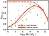 |
Fig. 2. Nuclear star cluster occupation fraction for our fiducial model as a function of galaxy stellar mass for all galaxies (solid line) and all galaxies hosting an MBH (dashed line). All M* < 109 M⊙ galaxies hosting an MBH have also a 100% probability of hosting an NSC at creation. The data represents the NSC occupation fraction for the Virgo (orange circles), Fornax (white squares), Coma (gray triangles) clusters, and the Local Volume (green rhombuses) as presented in Hoyer et al. (2021). Our model fits the logistic function for NSC occupation at M* < 109.5 M⊙ of the same work (thin gray line). We stress that this agreement occurs naturally from the occupation of MBHs per galaxy (see discussion in Sect. 4.2). |
2.2. From galaxy properties to time-dependent tidal eruption event rates with PhaseFlow
Black hole masses and the properties of the nuclear stellar component of galaxies, modeled in L-Galaxies BH as described above, provide the starting point for the calculation of time-dependent TDE rates.
The main, ubiquitous generation mechanism for TDEs is thought to be two-body relaxation (Chandrasekhar 1942; Frank & Rees 1976; Binney & Tremaine 2008). In simple terms, stars in the vicinity of an MBH deflect each other’s orbits so that a number of them may eventually reach a very small pericenter, closer than its tidal disruption radius, defined as
and be disrupted by the MBH of mass M•. Here, m⋆ is the stellar mass and r⋆ is its radius. The occurrence of these events can be described in terms of the "loss cone theory" (see e.g., Merritt 2013; Stone et al. 2020), adopting a Fokker-Planck approach to treat two-body relaxation. In particular, in the present work, we make use of the PHASEFLOW code (Vasiliev 2017), which is part of the AGAMA toolkit (Vasiliev 2019). PHASEFLOW evolves in time a phase space density profile assuming a spherical and isotropic distribution function f(E), by solving the Poisson and orbit-averaged Fokker-Planck 1D equations for the stellar distribution function, its gravitational potential, and its density. In general, two-body relaxation would induce an additional, explicit dependence of the distribution function on the angular momentum J of the orbit, which allows for the computation of the rate of stars being tidally disrupted. The rate of stars with energy E whose pericenter becomes smaller than the tidal disruption radius rt can be computed as the rate of stars whose angular momentum becomes smaller than  . At each energy, PHASEFLOW assumes the steady profile in angular momentum arising from relaxation (Cohn & Kulsrud 1978), and directly associates the isotropic profile f(E) to a (per energy) TDE rate. This results in an extra sink term in the energy-only Fokker-Planck equation and a growth term for the MBH mass. PHASEFLOW has been extensively used in the framework of inferring TDE rates, including addressing the impact of the stellar mass function on TDE rates (Bortolas 2022) as well as predicting realistically partial disruption event rates (Bortolas et al. 2023).
2.2.1. PhaseFlow setup
In our implementation, we assume that the stellar system surrounding the MBH is composed by a bi-chromatic population of stars made up of main-sequence stars of 0.38 M⊙ (encompassing ≈93% of the total stellar mass) and 16 M⊙ stellar black holes5 (encompassing the remaining ≈7%). Stars are considered to be destroyed if their separation to the MBH gets below rt (Eq. (3)), where we used r⋆ = 0.44 R⊙, which is the expected radius of a 0.38 M⊙ star (see e.g., Bortolas 2022, Eq. (3), for more details). Once accretion occurs, 30% of the stellar mass6 is added to the MBH, while the remainder is assumed to be lost in radiation and the interstellar medium. Stellar black holes are instead captured by the MBH if they get closer than 8GM•/c2 from the MBH, where c is the speed of light in vacuum and G the gravitational constant. During the evolution of the system, the stellar populations undergo the traditional dynamical phenomena expected in the vicinity to an MBH, that is, they develop a Bahcall & Wolf (1976) cusp, stellar black holes segregate in the center dominating relaxation in the closest vicinity to the MBH and finally, once the system reaches a dynamical equilibrium, expands and lowers its TDE rates as a result of dynamical heating. All these phenomena are captured by PHASEFLOW.
Given the fast performance of the code, we have generated multidimensional tables spanning a range of initial central MBH masses and a range of host-environment properties (mass, scale radius, compactness for disks, bulges, and NSCs), encompassing all values predicted by L-Galaxies BH, as described in what follows. In particular, all runs in the multidimensional grid were initially evolved for a Hubble time using 300 bins in the phase-volume, the variable used in the code to parameterize the distribution function7.
2.2.2. The PhaseFlow-generated grid of tidal eruption event rates
We modeled the rates depending on their reservoir origin, which could be either a bulge (or disk) or an NSC. Rates are saved in a large multidimensional grid, which includes the parameter space of the MBH, the stellar environment properties, and the time dimension. Rates are “not static” but instead vary with time (not necessarily a steady state is reached). This adds substantial realism to our computation, as many systems dominating the overall TDE rate are often characterized by a very large initial rate which drops by orders of magnitude with time. Assuming the static rate (which would coincide with the t = 0 rate) thus results in a non-negligible overestimation of TDE rates, especially for the case of NSCs.
The parameter space mapped is the following:
MBH mass. The first input parameter is the central MBH mass. The grid covers the range
![$$ \begin{aligned} \log _{10} (M_{\bullet }/M_\odot ) \in [2.5,8.0] \end{aligned} $$](/articles/aa/full_html/2024/09/aa49470-24/aa49470-24-eq9.gif)
in 34 equally spaced logarithmic steps. Here, the upper limit lies at the high-mass end of the event horizon suppression defined by the range of values of the Hills mass. The Hills mass is defined as the MBH mass for which the tidal radius is within the horizon radius (rt < rg, Hills 1975). The Hills mass depends on the black hole spin and the infalling star properties and its orbit (Kesden 2012; Mummery 2024), but it is in the range M• = 107 − 108 M⊙ for an 0.38 M⊙ star (see also Sect. 2.3.4).
Galaxy stellar component. To predict TDE rates, PHASEFLOW needs the galaxy stellar mass Mgal, the scale radius Rgal and Sérsic index ns. We mapped the stellar mass values in a broad range around the MBH mass M• values following this scaling:
![$$ \begin{aligned} \log _{10} (M_{\rm gal}/M_{\bullet }) \in [1,4] \end{aligned} $$](/articles/aa/full_html/2024/09/aa49470-24/aa49470-24-eq10.gif)
in 16 equally spaced logarithmic bins. The scale radius can instead vary in the range
![$$ \begin{aligned} \log _{10}(R_{\rm gal}/R_{\rm scl}) \in [-2,1] \end{aligned} $$](/articles/aa/full_html/2024/09/aa49470-24/aa49470-24-eq11.gif)
with 13 equally spaced logarithmic bins, where Rscl depends on the stellar mass as (Shen et al. 2003)

Finally, for the Sérsic index we assume all integer values between one and seven, which is the range we probe in L-Galaxies, as described in Sect. 2.1.3. This gives a grand total of 34 × 16 × 13 × 7 = 49 504 combinations of parameters for the galaxy stellar component. For galaxies with both a disk and bulge component, the contribution of the disk to TDE rates is ignored, as it is generally significantly lower. We note, however, that small galaxies in L-Galaxies BH are often pure disks, and their contribution to the total volumetric rate is non-negligible.
Nuclear star clusters. To estimate the TDE rates in an NSC environment with PHASEFLOW, the NSC mass MNSC, effective radius RNSC, eff and density profile are needed. Given the mass range for the galaxy component considered in the above grid (Eq. (5)), the NSC mass range follows by applying to this the scaling relation presented in Eq. (1) (from combining the works of Pechetti et al. 2020 and Hoyer et al. 2023). From Pechetti et al. (2020) we also used the definition of the NSC effective radius, which correlates with the galaxy stellar mass M* as

We stress that this relation is especially holding toward the high-mass end but flattens out at low masses (Neumayer et al. 2020). To explore how the results presented in this work depend on the choice of fixed compactness of the NSC, we construct a second grid using Reff, NSC equal to 1/3 of the radius predicted by the scaling relation. We dub these additional runs as compactNSC. The fiducial model follows Eq. (8) and will be compared with the compactNSC one in Sect. 4.4.
The initial NSC density profile was assumed to follow the functional forms of Saha (1992) and Zhao (1996):
![$$ \begin{aligned} \rho _{\rm NSC}(r) = \rho _0\left(\frac{r}{a}\right)^{-\gamma }\left[1+\left(\frac{r}{a}\right)^{\alpha }\right]^{\frac{\gamma -\beta }{\alpha }}\exp {\left[\left(-\frac{r}{r_{\rm cut}}\right)^{\xi }\right]}, \end{aligned} $$](/articles/aa/full_html/2024/09/aa49470-24/aa49470-24-eq14.gif)
where ρ0 is a normalization constant that ensures the total mass of the cluster is MNSC, a = RNSC, eff/4.6 is its scale radius, while α = 4, β = 2, and γ = 0.5 are respectively the outer, intermediate and inner density slopes. Finally, rcut = 12a is a cutoff radius and ξ = 2 represents the cutoff strength. The selected values have been chosen based on the results by Antonini et al. (2012), who explored the formation of NSCs through the infall of star clusters (see e.g. Capuzzo-Dolcetta 1993; Hartmann et al. 2011; Arca-Sedda & Capuzzo-Dolcetta 2014; Sánchez-Janssen et al. 2019; Fahrion et al. 2022; Carlsten et al. 2022; Leaman & van de Ven 2022; Hoyer et al. 2023, on the connection between NSCs and globular clusters). This profile should thus be a valid resemblance to the profile of a recently formed NSC.
Taking into account the scaling relations described above, it is clear that all NSC properties ultimately depend only on the galaxy stellar mass M*. Thus, the grid for the TDEs due to NSCs spans only the values of M• and M*, in the same ranges as mentioned for the galaxy stellar component above: total 34 × 16 = 544 pairs of parameters.
Once the runs with PHASEFLOW are completed and the grid in the parameter space has been fully mapped, we store the resulting event rates, Γ, which are a function of the aforementioned parameters and time t. For the bulge and disk contribution, the rates are encapsulated in the function Γgal(Mgal, Rgal, ns; M•, t), while for the NSCs, the rates are given by the function ΓNSC(MNSC; M•, t). We stored the rates differently for late times,
![$$ \begin{aligned} \log _{10} (t /\mathrm{yr}) \in [7.0,10.146], \end{aligned} $$](/articles/aa/full_html/2024/09/aa49470-24/aa49470-24-eq15.gif)
and for early times,
![$$ \begin{aligned} \log _{10} (t /\mathrm{yr}) \in [1.0,7.0], \end{aligned} $$](/articles/aa/full_html/2024/09/aa49470-24/aa49470-24-eq16.gif)
with 50 and 60 evenly spaced logarithmic bins, respectively, for the two time ranges. We considered separately the TDE rates at times below 107 yrs given the time resolution of L-Galaxies BH, which spans between dtstep ∼ 5 − 20 Myr, depending on redshift. Specifically, for MBH mass M• < 106 M⊙ the peak TDE rate due to NSCs falls below the time resolution of L-Galaxies BHdtstep ∼ 10 Myr; therefore, the initial phase of high TDE rates and growth (dubbed here as “prompt phase”) would not be treated properly by our model (see Fig. 3). To resolve that, when the TDE phase due to NSCs is initialized for these small MBHs, we draw a random time between 1 and dtstep and assign rates from the prompt phase tables according to this time. At the same time, we add the integrated mass during the unresolved prompt phase to the MBH.
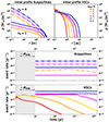 |
Fig. 3. Density profiles for different MBHs and the resulting time-dependent TDE rates. Top panels: stellar density profiles for a range of MBH masses as indicated in the inset legend (with the same color coding applying to all panels of the figures). Disks have been assigned nS = 1 Sérsic profiles (solid lines, left), while bulges have nS = 4 profiles (dotted lines, left). The NSCs were instead assigned spheroid profiles from Eq. (9) (right). The galaxy and NSC host properties scale with M• as described in the text and are created to be representative of the average environment encountered in L-Galaxies BH. Middle and bottom panels: tidal disruption event rate evolution with PHASEFLOW when initiating for different MBH mass with the associated profiles from the top panels, displayed separately for bulges or disks (galaxy component, middle panel) and NSCs (bottom). The gray region below 10 Myr indicates the region where we trace unresolved growth and high-rates below the time-resolution dtstep for the black holes in NSCs with mass M• < 106 M⊙. This initial phase we refer to as prompt phase. |
In the following section, we outline how we merge L-Galaxies BH with the Γgal and ΓNSC rates constructed from the multidimensional grid described above. To guide the reader, Fig. 3 shows several examples of the time-evolving TDE rates for a variety of black hole masses and for a fixed set of parameters. In the figure, for each black hole mass, we assume that the corresponding galaxy stellar mass is given from the relation log10 (M•/107.43 M⊙) = 0.62log10(Mgal/1010.5 M⊙), which is the best-fit relation we get in L-Galaxies BH at z = 0 for MBHs up to ∼108 M⊙. The scale radius assigned to the Sérsic profile is here assumed to be an average value of Rgal = Rscl. The disk corresponds to ns = 1 and the bulge to ns = 4. The matching NSC profiles are created by using the scaling relations presented in Eqs. (1) and (8).
As shown from Fig. 3, the main general feature of our model is that the typical, average rates increase with increasing MBH mass, as the stellar reservoirs assigned are increasingly more massive for more massive MBHs. However, there is a strong differentiation between the galaxy component and the NSC component; while bulge and disk profiles often obtain a constant event rate given the large relaxation timescale of these systems, NSCs matching to M• < 106 M⊙ show decay in their initial TDE rate due to their fast relaxation dynamics. Typically, the decay happens earlier for smaller MBHs and smaller reservoirs. Notably, NSCs with M• from 104 M⊙ to 106 M⊙ start with similar TDE rates at 107 yrs, but maintain it shorter times compared to the Hubble time, as the systems quickly reach their equilibrium in the form of a Bahcall & Wolf (1976) cusp and subsequently expand due to the dynamical heating resulting from efficient relaxation. That proves the importance of including the analysis of the initial rates that fall below L-Galaxies BH time resolution.
2.3. Tidal disruption event rates in L-Galaxies
The final step consists of joining in a self-consistent way the TDE rates calculated by PHASEFLOW and the properties and stellar environments of MBH predicted by L-Galaxies BH. We schematically show this in Fig. 4, and we describe the details below.
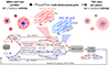 |
Fig. 4. Flowchart of the current scheme for estimating TDEs within a single time step of L-Galaxies BH. The decision-making tree is colored red and blue for the galaxy (bulge or disk in the absence of bulge) and NSC components, respectively. With the density profile ρgal we refer to all galaxy component parameters {Mgal,Rgal,nS} that are used to initialize the Sérsic profile. TDE rates from the galaxy as a whole and its NSC are effectively treated independently (each process has its clock ΔtTD) and can be active at the same time, while they sum together to produce the instantaneous rate of each MBH. |
2.3.1. Event rates and mass accretion
As soon as an MBH forms inside a galaxy in L-Galaxies BH, we set a TDE rate depending on the existence of a stellar bulge (or disk) and/or an NSC. Effectively, we look up the multidimensional grid generated with PHASEFLOW for the rate Γi, with i = gal for the galaxy component and i = NSC for the NSC. From this, we derive the time-evolving rates for each MBH and stellar environment. For galaxy and NSC properties we look up for the closest values in the grid, while we interpolate in the MBH and time dimension8.
When TDEs start being produced within a galaxy, either from the relaxation of the bulge (or disk) or the NSC, we start a clock, ΔtTD, i. In the successive steps of the L-Galaxies BH run, the PHASEFLOW grid is checked at the corresponding subsequent times. As described in the next section, we reset this clock to zero only when the MBH and/or the galaxy have substantially changed, which can happen, for example, after mergers.
Next, we define the fraction of the stellar mass accreted by the MBH after it has been tidally disrupted:
 In reality, around the Hills mass both direct captures and disruptions could take place, depending on the orbit of the infalling star9, but we did not expect this to change our results for the TDE rates or the BH growth, which in this mass range is dominated by gas growth anyway10
Provided the TDE rate and the accretion fraction f*, TDE per event, the mass accreted by the central MBH from each stellar component11 during each time step of L-Galaxies BH is given by:

and the mass subtracted (i = gal or i = NSC) is:
![$$ \begin{aligned} \mathrm{d} M_{i, \mathrm{loss}}= \mathrm{d}t_{\rm step} \left[ \, \Gamma _{i} (+ \Gamma _{\rm NSC} \;\mathrm{if}\,i=\mathrm {gal}) \, \right] \,m_*. \end{aligned} $$](/articles/aa/full_html/2024/09/aa49470-24/aa49470-24-eq19.gif)
Notice that, if both a bulge (or disk) and an NSC are present, we sum the two TDE rate contributions. The results of the mass growth of MBHs through this mechanism are discussed briefly in Sect. 4.1.
2.3.2. Conditions for resetting tidal disruption event rates
As mentioned above, PHASEFLOW is able to capture the time evolution of the stellar density profile as a result of relaxation and MBH growth due to star accretion. Thus, once TDEs start taking place within a galaxy in L-Galaxies BH, we follow their time evolution based on the grid provided by PHASEFLOW.
However, dramatic events, such as mergers, disk instabilities, and starbursts, can lead to major changes in the stellar environment surrounding the MBH. In these cases, we reset the clock for TDE rates (ΔtTD, i), and the new, unrelaxed stellar system starts again evolving toward a new relaxed state until the next violent dynamical event. The conditions under which we considered it relevant to check the state of the TDE process taking place around an MBH are the following:
Changes in MBH mass. If the mass accreted by the MBH via gas accretion is three times larger than the mass accumulated from TDEs, then the ΔtTD, NSC clock is reset again and the NSC mass and properties are adapted to the galaxy stellar mass at that time12. For bulges(or disks), rates are less time-dependent (see discussion in Sec. 2.2), so we omit this condition.
Changes in the galaxy component mass. If during one L-Galaxies time step the bulge or disk stellar mass increases by more than 20%, the clock ΔtTD, gal is reset. Such variations in stellar mass in a short amount of time is a typical change in post-starburst galaxies (Kaviraj et al. 2007; van Velzen 2018; Wild et al. 2016, 2020). We note that events that do not modify the total stellar mass can also lead to a reset of the rates (e.g., the transfer of mass from the disk to the bulge during disk instabilities).
Changes in NSC mass. We do not expect all changes of the galaxy component to affect the TDE rate evolution in NSCs, since these can continue relaxing at their own pace unaffected by the changes at larger galactic scales. However, as described in Sect. 2.1.4, an NSC can undergo significant mass changes following the host galaxy changes. Following the same approach described above, we select that NSC that grow more than > 20% within one L-Galaxies BH time step will satisfy the condition of resetting the clock ΔtTD, NSC. This threshold is selected to be equal to that of the galaxy component in order to minimize the free parameters of the model.
Changes in NSC to MBH mass ratio. While there are no clear constraints on the limits of the mass ratio between an NSC and the MBH at its center, namely 𝒟 = MNSC/M•, we decided to put a lower limit on this ratio so that an NSC gets to be (re)generated only if 𝒟 > 𝒟nuc. Only a few physically motivated arguments can provide some insight for the allowed value of 𝒟: a) MBHs cannot be arbitrarily massive if they form in the cluster, for instance, simulations of runaway stellar collisions by Kritos et al. (2023) indicate that 𝒟 > 1, and b) the NSC destruction from binary MBHs, for example, total and partial disruption of clusters from intermediate-mass MBH binaries, takes place for values 𝒟 < 5 and < 15, according to Khan & Holley-Bockelmann (2021). Given the theoretical uncertainties of the NSC-MBH symbiosis and provided local NSCs are observed with even lower values (𝒟 ∼ 0.01, Neumayer & Walcher 2012), we select conservatively 𝒟nuc = 0.1. We stress that this parameter (along with M*, NSC cut-off) can be later substituted from a physically motivated formulation when the NSC model is implemented in L-Galaxies BH by Hoyer et al. (in prep.).
We have checked that variations within an order of magnitude of the thresholds mentioned above do not significantly affect the results on the volumetric rates presented in this work. However, we will further discuss some of these assumptions in Sect. 4.4.
2.3.3. Treatment of tidal eruption event in active galactic nuclei
When MBHs experience phases of gas accretion, they shine as active galactic nuclei (AGN). These phases can be coeval with events of stars disruptions. The two processes may not be completely unrelated to each other. For instance, it has been proposed that TDE rates can be enhanced due to the alignment of retrograde orbits of NSC stars with the MBH accretion disk (Generozov & Perets 2023; Nasim et al. 2023), due to the turn-off of the disk (Wang et al. 2024), or due to the quadrupole moment of the disk modifying the loss cone (Kaur & Stone 2024). However, by construction, our model does not account for this possible rate enhancement since gas physics are not included in PHASEFLOW. Regarding the impact of TDEs on the AGN disk, the few TDE interpretations of fast flares in AGN light curves suggest a (temporal) post-flare increase (Blanchard et al. 2017; Liu et al. 2020) and others a decrease (Cannizzaro et al. 2022; Cao et al. 2023) of the AGN luminosity. Given the high uncertainty, we assume that the disk recovers quickly (compared to the time to the next TDE) or is not interrupted at all by TDEs so that both the TDE and AGN luminosity are kept as independent properties of each MBH. We do not expect this assumption to affect the global rates, due to the small AGN fraction at z ∼ 0 (< 10% of MBHs are active) unless the TDE rates are significantly boosted in the presence of an accretion disk (by a factor of 10 or greater).
2.3.4. From simulated to observable tidal disruption event rates
Once TDEs are carefully linked to the MBHs and their galaxies evolving within L-Galaxies BH, we need to transform the individual rates to observable events to finally compare our predictions with the events picked up by time-domain surveys. Here we keep the following minimum number of assumptions to translate simulated TDE rates to observed ones:
-
We assume that all TDE events are full disruptions. In reality, for massive stars, only those with a pericenter that is a fraction of the tidal radius are fully disrupted (otherwise they are partial), and the energy output of the events may depend on the penetration factor of the star. Moreover, provided that a handful of partial disruption events have been identified (Payne et al. 2021; Malyali et al. 2023), we discuss the impact of such a choice in Sect. 5.
-
We assume that all TDEs give a luminosity that falls within the sensitivity of current surveys, i.e., all events are detectable, if there is no AGN contribution. If there is no AGN contribution. In the presence of an AGN, we ignore TDEs in MBHs with AGN bolometric luminosity Lbol > 1042 erg/s (fiducial model) unless noted otherwise. We also note that we do not include any obscuration and line-of-sight effects.
-
Regarding the event horizon suppression, the predicted TDE rates for each MBH are considered either visible or not depending on the Hills mass of the black hole itself. The Hills mass depends on (i) the mass M• and spin χ• of the MBH, (ii) the age of the loss-cone since the cluster/galaxy component was last reset ΔtTD, i and (iii) the mass of the infalling star. For this last point, we draw the stellar mass m* of the disrupted star from a truncated Kroupa mass function (m* < 1.5 M⊙). Given the values above, each MBH is assigned a Hills mass MHill(m*, ΔtTD, i, χ•) based on the tabulated results of Huang & Lu (2024, Table D1) who have performed a series of simulations of solar-metallicity stars disrupted by MBHs13. If M• > MHills, we omit this MBH from the sum of the bulk rates. Otherwise, we assume that all events are full TDEs and have the rate assigned to the MBH14.
Note also that, given the mass resolution of the dark matter simulation used and of the multidimensional grid of TDE rates, we omit from the analysis the TDE rates from galaxies with masses M* < 105.5 M⊙ and/or MBHs M• < 102.5 M⊙. Finally, we note that given all the assumptions above, the volumetric rates presented below can be considered optimistic.
3. Results
In this section, we present our main results on the predicted TDE rates for the fiducial choice of parameters and how they compare with the TDE rates observed by the latest time-domain campaigns. We also discuss the implications of our model for the time evolution of TDE rates and the general properties of the MBHs and galaxies hosting TDEs. The interpretation of the results in view of the population of NSCs and MBHs, the implications for MBH spin and growth through TDEs are discussed later in Sect. 4.
3.1. Volumetric tidal disruption event rates
In Fig. 5, we present our predictions for the volumetric rates as a function of MBH and galaxy stellar mass for our fiducial model, comparing them with the recent constraints of Yao et al. (2023) derived from a sample of 33 TDEs from the ZTF survey. As shown in the left panel of Fig. 5, our model can reproduce the overall shape of the volumetric rates, including the flattening at intermediate MBH masses and the drop for M• > 106.5 M⊙. Yao et al. (2023) also derived a simple model for the volumetric rates as a function of MBH mass using the Gallo & Sesana (2019) and Shankar et al. (2016) mass functions and including the event horizon suppression (dotted-dashed lines in the left panel of the figure), and our predictions are in overall agreement with these models.
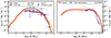 |
Fig. 5. Volumetric TDE rates per black hole (M•, left) and galaxy (M*, right) log mass at z = 0.0 for the fiducial model (solid line). Our model is compared against the constraints (here plotted with the error range) from Yao et al. (2023) for all MBHs (left) and all galaxy types (right). For reference, we display the previous constraints from van Velzen (2018) and the luminosity function from Sazonov et al. (2021) transformed to a mass function (see the details in the text). We also display the model lines of Yao et al. (2023) for the TDE rates as a function of a) MBH mass, assuming the Shankar et al. (2016, maroon shorter dash-dotted line; Sh16) and the Gallo & Sesana (2019, cyan long dash-dotted line; G19) MBH mass functions, which both include the event horizon suppression, and b) galaxy stellar mass, obtained by multiplying the galaxy stellar mass function with the power-law dependence of rates on |

We note that the higher normalization with respect to Yao et al. (2023) at intermediate masses (M• = 105.5 − 107 M⊙) is due to the presence in our model of many black holes in this mass range in dwarf galaxies (M* = 106 − 109 M⊙), which is a stellar mass range still not constrained by current datasets (however, see discussion on partial disruption events in Sect. 4). Also, Yao et al. (2023) assign to the detected events black hole masses based on the M•–σ* relation from (Kormendy & Ho 2013), which predicts smaller MBH masses in the low stellar mass regime with respect to the predictions of our model and the observational results of, e.g., Reines & Volonteri (2015). Alternatively, we could obtain a lower normalization in the volumetric rates at intermediate masses by decreasing the MBH and/or the NSC occupation fraction or allowing smaller NSC masses in the model (as discussed in Sect. 4.2). Moving to the low-mass regime (M• < 105.5 M⊙), we find that the turnover is due to lower average NSC masses and greater ages around small MBHs (which translates into significantly reduced TDE rates by z = 0).
Our results are also broadly in agreement with the volumetric rates as a function of MBH derived from the eROSITA X-ray luminosity function assuming an Eddington-limited accretion and a simple volumetric correction15 of kbol = 15. The two classes of optical-UV and X-ray TDEs might not be eventually different as inferred from recent studies (Guolo et al. 2024), so we anticipate the two mass functions to be similar (which is the case within errors with the simple transformation we performed). Finally, in the left panel of Fig. 5 we also plot the previous constraints from van Velzen (2018) for reference. These are higher than both the model predictions and the Yao et al. (2023) constraints at all MBH masses below event horizon suppression. This could be due to the smaller number statistics (17 TDEs) and the heterogeneous nature of the van Velzen (2018) sample (see discussion for the low-end of the luminosity function, Yao et al. 2023).
In the right panel of Fig. 5 we present again the model predictions of the volumetric rates, but now as a function of the host-galaxy stellar mass, M*. As shown, our predictions at z = 0 display a broad agreement with the shape of the distribution from Yao et al. (2023).
To describe the distribution of observed TDEs, Yao et al. (2023) derive a model using the galaxy stellar mass function coupled with a power-law dependence of the rates on galaxy stellar mass ( , originally from the rate dependence on MBH mass
  , with B = −0.25). A similar functional form has been used previously, e.g., for various local galaxies (Wang & Merritt 2004), and for galaxy central cores and cusps (Stone & Metzger 2016). In the range M* = 109.5 − 1010.5 M⊙ our model prediction can be fitted with a similar power law, but we predict a different functional form at the low mass end.
3.2. Per-galaxy tidal disruption event rates
In Fig. 6, we show the per-galaxy TDE rates as a function of MBH mass (left panel) and stellar mass of galaxies hosting an MBH (right panel). We further split the contributions to the total TDE rates from NSCs and the galaxy component16, further subdivided into old (ΔtTD > 3 Gyr) and young (ΔtTD < 30 Myr) systems. We immediately see that the contribution of NSCs to the total rates dominates across all masses. The rates from the galaxy component increase both with MBH and galaxy stellar mass up to the event-horizon suppression mass. However, they are on average more than three orders of magnitude lower when compared to the contribution from the NSC at fixed MBH/host galaxy stellar mass. This result has important implications for the expected nucleation fraction of galaxies, which we will further discuss in Sect. 4.2. Indeed, based on these results, TDEs should be predominately observed in the presence of NSCs. Current observations of TDEs are primarily from distant enough sources where NSCs remain unresolved.
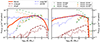 |
Fig. 6. Average TDE rates per log mass of MBH M• (left) and of the MBH host galaxy M* (right) for the fiducial model at z = 0.0 (solid red line, tagged as “all”). We averaged separately over NSC rates (light-blue lines) and galaxy component rates (maroon lines), and subsequently split into just restarted (“young” systems with ΔtTD < 30 Myr, dashed line) and after a long time (“old” systems with ΔtTD > 3 Gyr, dotted lines). For comparison, we present the results of (Pfister et al. 2020) for three different scaling relation pairs of MBH galaxy stellar mass and NSC mass size adopted in their work (DD, DP, and KD as defined in Table 2 of Pfister et al. 2020) to bracket the uncertainties following these hypotheses. |
When looking at the difference between old and young systems, we see a different behavior for the NSCs and the galaxy contributions. Recently formed NSCs give the highest contributions to the per-galaxy rates, with approximately constant values of ∼10−5 yr−1 per MBH/galaxy (see the bottom panel of Fig. 3, where we showed that M• = 104 − 107 M⊙ have similarly high rates at t = 107 yr). Instead, old systems below M• < 107 M⊙ exhibit a power-law dependence on MBH mass, namely  with B = 1 (compared to B = 0 for young systems under the same definition). The old NSCs have on average small mass compared to their MBH. For these systems, the relaxation time becomes significantly short, thus the loss cone gets quickly depleted. In the low mass regime (M• < 105 M⊙), the majority of systems have rates from old rather than young NSCs and that is why the global per-MBH rates drop toward lower masses. This has specific implications for the dwarf galaxy regime (yet to be probed with observations), where per-MBH/per-galaxy TDE rates are higher by a factor of > 10 for young NSCs over old NSCs. Therefore, our work suggests that a promising opportunity of sampling TDEs is selecting recently interacting systems, with a predicted per-galaxy (volumetric) rate of ∼1 × 10⁻⁵ yr−1(∼1 × 10⁻⁷ yr−1 Mpc−3 dex−1). This prediction holds down to the least massive dwarfs, as marked by the flattening of the rates as a function of galaxy stellar mass (for both per-galaxy and volumetric TDE rates, see respectively the right panels of Figs. 5 and 6). This revision of rates in dwarf galaxies may have a significant impact on theoretical predictions of TDEs in intermediate-mass MBHs. The galaxy contribution shows a different behavior with age. First of all, we note again that TDEs from the galaxy component do not strongly depend on time and that bulges lead to larger rates compared to pure disks (see discussion of Fig. 3 in Sect. 2.2). In Fig. 6, we see that old systems have higher per-galaxy rates with respect to the young galactic components at the lower MBH M• < 106.5 M⊙ and galaxy M* < 108 M⊙ masses. We attribute this to the morphological differences between old and young galaxies in this mass range: L-Galaxies BH predicts that young systems are mostly pure disks (with an average bulge-to-total mass ratio of ⟨B/T⟩ = 0.075), while old systems are preferentially bulge-dominated (⟨B/T⟩ = 0.3). At the high mass end, instead, we see that young galaxies have higher per-galaxy rates than old ones as a function of galaxy stellar mass. In this case, the difference can be attributed to the differences in the M• − Mgal ratio for young and old systems: at fixed galaxy stellar mass as an effect of early on-set of MBH growth, old systems are preferentially hosting heavier MBHs, whose galaxy-component rates are lower. In both cases the per-galaxy rates follow a power law of the form
  with B ≈ 0.7 for the mass range M• = 106 − 108 M⊙ and M* = 108 − 1011 M⊙.
We then compared our model predictions in Fig. 6 with the ones of Pfister et al. (2020), who motivated by the computation of TDE rates in observed galaxy profiles, computed the per-galaxy TDE rates for a mock catalog of galaxies hosting NSCs and with a well-characterized bulge component. Before making a comparison, it is worth noticing that Pfister et al. (2020) derives MBH masses using, also in the low-mass regime, M• − M* scaling relations observationally derived for massive spheroidal galaxies (Kormendy & Ho 2013; Davis et al. 2019). Moreover, although they use PHASEFLOW to compute the TDE rates, they assume a monochromatic star distribution of m* = 1 M⊙, while this work uses m* = 0.38 M⊙ and stellar black holes (16 M⊙), a difference that can change by a factor of two the number of stars entering the loss cone, thus available for TDEs (Stone & Metzger 2016).
The per-galaxy rates for NSCs (solid red lines) are consistent with the predictions of Pfister et al. (2020) for M• > 106.5 M⊙ and M* > 1010 M⊙ but have a different trend (they diverge) at lower masses. We suspect that the main difference to the rates toward lower masses is the use of steep Sérsic profiles nNSC for low mass NSCs, using the scaling relation of Pechetti et al. (2020) (for MNSC < 106 M⊙ the relation gives Sérsic indices with values above 4). This anticorrelation between NSC mass and Sérsic index for lower masses appears to be weaker in the recent results of Hoyer et al. (2023). We instead assume shallower, possibly more realistic, profiles, as described in Sect. 2.2 and no correlation of the steepness of the profile with mass. Moreover, Pfister et al. (2020) do not allow for small structures with M• > MNSC, while there is evidence of such objects and they are naturally included in our model (see Sect. 4.4 for the impact of this parameter).
Regarding the TDE rates from the galaxy component, Pfister et al. (2020) also finds an increase both with MBH and galaxy stellar mass until the event-horizon suppression mass. Nevertheless, the average rate they predict is three to four orders of magnitude higher than our predictions for all galaxy stellar mass ranges. This is probably because Pfister et al. (2020) assumes on average more centrally concentrated galaxies compared to our work. Also, as mentioned earlier, at the low galaxy stellar mass end, they assign MBH masses using the same steep relation as for a more massive system: this implies that, at fixed MBH mass, their stellar mass can be up to 2 dex larger than ours.
The results just discussed highlight that the demographical analysis of TDE rates requires a realistic cosmological environment with carefully constructed morphological galaxy properties and number distributions as a function of galaxy stellar mass, that L-Galaxies BH provides.
3.3. Redshift evolution of tidal disruption event rates
Having captured the z = 0 global rates, we now discuss their redshift evolution and how that compares with the evolution of the underlying MBH properties and their environment.
In Fig. 7 we display the volumetric TDE rates for redshifts z = 0, 1, 2. Regarding the case of TDE rates as a function of MBH mass, there does not seem to be a significant change in the rates between z = 0 and z = 1. This is due to the very mild evolution evolution predicted by the model for z < 1. This result is in line with the general assumptions that the volumetric TDE rates do not evolve significantly with redshift (see e.g.van Velzen & Farrar 2014; van Velzen 2018; Yao et al. 2023 see, however, the approach of Kochanek 2016). Despite this, there is a slight decrease of half an order of magnitude when comparing resolved TDEs at z = 0, 1 and z = 2, which will be an important feature to study with deep sky surveys such as LSST (Hambleton et al. 2023; Bricman & Gomboc 2020; Bučar Bricman et al. 2023) and UV transient surveys like QUVIK (Zajaček et al. 2024). However, it is worth mentioning that our predictions are model-dependent. We assume that MBHs are always associated with an NSC at all redshifts (see Sect. 2.1.4). If this was not true at early times, high-redshift TDE rates would be lower.
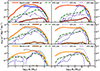 |
Fig. 7. Redshift evolution [z = 0 (top), z = 1 (middle), and z = 2 (bottom)] of the volumetric TDE rates per MBH (left) and stellar (right) mass originating from all low-luminosity or inactive MBHs (cutoff at log10LAGN [erg/s] < 42 for the fiducial model, solid lines) and TDE rates from the galaxy components only bulges (or disks); solid lines tagged as “gal”). We also display the rates only from AGN-hosts with "high" (purple dashed-dotted), "moderate" (green dashed), and “low” (blue dotted) luminosity (log10LAGN [erg/s] ∈ [42, 45], [40.5, 42] and [39, 40.5] respectively). The z = 0 constraints Yao et al. (2023) are plotted in all panels for reference (with gray when they do not apply). These fractions remain qualitatively the same for these redshifts for most of the parameter variations. |
The volumetric rates shown in Fig. 7 can be divided into contributions from the galaxy component (“gal”) and the NSC. The first, although it steadily increases from z = 2 to z = 0 with the increase of bulges in galaxies, still provides a negligible contribution to the volumetric TDE rates at all masses and all redshifts. In practice, the volumetric rates are entirely due to galaxies hosting NSCs (this contribution is not shown in the figure as it essentially coincides with the total “fiducial” volumetric TDE rates). While the per-galaxy rates for NSCs remain the same at high masses toward higher redshifts, there is a slight enhancement (by a factor less than three) compared to z = 0 for M• < 106 M⊙ MBH and M* < 109 M⊙ host-galaxy stellar masses, because of continuous reset of TDE rates during frequent mergers at cosmic noon. This somewhat counteracts the decrease of the number density of inactive MBHs toward higher redshifts and results in a moderate evolution of the volumetric TDE rates.
3.4. Tidal disruption event rates in active massive black holes
Searches for TDEs in AGN at optical (Dgany et al. 2023, ZTF) and X-ray (Homan et al. 2023, eROSITA) wavelengths have not yielded many representative cases. However, observations of luminous ambiguous nuclear transients (Frederick et al. 2021; Hinkle et al. 2022; Oates et al. 2024), TDEs and TDE-like flares in ongoing/previous AGN (Li et al. 2023; Huang et al. 2023; Makrygianni et al. 2023; Charalampopoulos et al. 2024), and changing-look AGN (Ricci & Trakhtenbrot 2023; Zhang 2022) hint that the two TDE and AGN activity could be related. So far, few theoretical works (Karas & Šubr 2007; Chan et al. 2019; McKernan et al. 2022; Prasad et al. 2024) and recent simulations (Ryu et al. 2024) have explored the coexistence of TDEs and AGN. Predicting TDEs in AGN hosts is beyond the scope of this paper, as it requires dedicated modeling of the electromagnetic emission of individual events, considering the relative brightness of TDEs and their host. This section overviews TDE occurrence in AGN under the assumptions outlined in Sect. 2.3.3, aiding future searches for transient events in AGN.
In Fig. 7 we show the volumetric global rates at z = 0, 1 and 2, for MBHs triggering AGN with low, moderate and high bolometric luminosity bins: log10 (Lbol [erg/s]) ∈ [39.0, 40.5], [40.5, 42.0] and [42.0, 45.0]. We note that for high AGN luminosity, the detectable rate of events will depend on the luminosity of individual TDEs. In other words, only TDEs with peak luminosity significantly higher than the AGN luminosity at a given wavelength would allow the characteristic time decay of a TDE light curve to be distinguished, thus singling out the event from AGN stochastic variability or unrelated flaring activity. The first thing to notice in Fig. 7 is that the strong redshift evolution of the AGN luminosity function leaves an imprint on the AGN hosting TDEs. Indeed, the lower the redshift, the greater the importance of inactive MBHs in the volumetric TDE rates. This is because a large fraction of massive black holes consume their high-z gas reservoir and end up in an inactive phase in the low-z Universe.
We observe that at high MBH and host-galaxy stellar masses (M• > 108 M⊙ and M* > 1010.5 M⊙) and at all redshifts, the volumetric rate of TDEs occurring in luminous AGN (all luminosity bins) is comparable to the one occurring in inactive or low activity AGN (fiducial) curve and almost redshift-independent at Gpc−3 yr−1 dex−1. Specifically for redshift z = 2, the TDE rates of luminous AGN (high) dominate over the rates of low-activity MBHs at host-galaxy stellar masses M* > 108 M⊙ and M• ∼ 106.5 M⊙ MBHs. Therefore monitoring flares in AGN at z > 1 might be an effective way to identify TDEs, assuming that a significant fraction of TDEs will be brighter than the AGN emission itself.
4. Discussion
Here we address the implications of the inclusion of TDEs for the modeling of MBHs with L-Galaxies BH, and explore how the results presented in this work are affected by the parameters and assumptions of our model (Section 2).
4.1. Massive black hole growth via tidal disruption events
As mentioned in the Introduction, the role of TDEs in the mass content of MBHs has been so far theoretical, with no means to calibrate this mechanism at analytical prescriptions of this MBH growth channel. Since our work already is in broad agreement with the TDE rates at z = 0, we can draw some first conclusions on the contribution of TDE rates to the growth of the MBH population. Here we limit the discussion to the impact of TDE on the growth of the MBH population by z = 0. Another important aspect regarding growth is the time resolution; according to Broggi et al. (2022) MBHs residing in NSCs will double their mass within a characteristic timescale that depends on the MBH mass (in their set-up, they have a power-law dependence 1.29) and falls below time resolution for MBHs M• < 105 M⊙. We include the prompt phase by integrating the rates taking place below the time-resolution dtstep. A more detailed investigation of the conditions for efficient growth via TDEs and of the sub-categories of galaxy types where and when this growth channel is important will be the subject of follow-up work (Polkas et al., in prep.).
In Fig. 8, we show the fractional cumulative mass content of MBHs, namely fBHAM17 at z = 0 as a function of their mass, for the runs with and without prompt phase. As demonstrated in these plots, the mass growth through TDEs is mostly insignificant for the high mass ranges (i.e., fBHAM < 1% for M• > 105 M⊙), especially when compared to the mass growth induced by cold gas accretion. However, for MBHs that remain close to their seed mass M• = 102.5 − 105 M⊙, TDEs offer a competitive channel of growth, composing fBHAM = 1 − 10% of their mass. Notably, for the lightest mass bin M• < 103 M⊙, TDE growth is as important as the cold gas accretion, the latter being less significant (if at all existent) in dwarf galaxies (see Figs. 7 and 10 of Izquierdo-Villalba et al. 2019; Spinoso et al. 2023, respectively). Regarding this result, we nonetheless stress the theoretical uncertainties regarding the position and residence time of MBH seeds in the centers of galaxies and the NSCs that may diverge from the physics included in L-Galaxies BH regarding more massive MBHs.
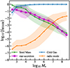 |
Fig. 8. Average fraction of mass accreted by different MBHs at z = 0 (fBHAM) via stellar captures (purple squares), cold gas accretion (blue right triangles), hot gas accretion (orange left triangles), and accumulated seed mass (green circles) without (top panel) and with (bottom panel) an initial prompt phase (see main text). The margin of ±1 standard deviation of log10fBHAM for each type of channel is highlighted with the same-color shaded area. |
For the relative massive MBHs at z = 0 (M• > 106 M⊙), their seeds grow through gas accretion to M• = 104 − 106 M⊙ by z = 2 − 3, allowing for important cumulative TDE growth (after the initial gas growth) until z = 0. This is shown by the ‘excess,’ which brings the star-accretion curve over the seed mass one (for MBHs with M• = 104.5 − 107.5 M⊙). Both M* and MNSC will be greater for MBHs of this mass range, resulting in constant high rates with time compared to those of surviving dormant seeds living in isolation. The latter cannot maintain a constant high rate as indicated by the per-MBH rates for old NSC systems in Fig. 6. More massive MBHs (M• ∼ 108 M⊙) form early in the most massive galaxies (M* ∼ 1011 M⊙) of the simulation, and they will stop being hosted in NSCs earlier and grow less through TDEs.
Our results add realism to estimates from earlier works. Unlike claims using the full loss-cone theory (e.g. Milosavljević et al. 2006; Alexander & Bar-Or 2017), the growth via TDEs in our model is not such that all M• < 104 M⊙ MBHs would reach the supermassive regime as a result of stellar accretion. We attribute this behavior to a) the vast majority of low-mass MBHs being hosted in lower-mass galaxies with less massive NSCs and b) the time-dependent nature of the rates; noninteracting ancient NSCs relax quickly and can even become less important than the bulge and disk rates (see input rates Fig. 3). As mentioned above, however, we will study in a follow-up work the specific properties of the environment and redshifts that lead to more efficient growth via TDEs.
4.2. Implications for massive black hole and nuclear star cluster populations
Complete galaxy samples are starting to constrain the AGN occupation fraction across different galaxy stellar masses, hinting at significantly smaller AGN fractions in dwarf galaxies (i.e., < 10−2) than in massive systems (see e.g. Mezcua et al. 2018; Mezcua & Domínguez Sánchez 2020; Bykov et al. 2024; Zou et al. 2023; Siudek et al. 2023). This could be explained if the number of AGN in dwarf galaxies remains small because of the lack of cold gas in the center of these systems (Urquhart et al. 2022), which cannot sustain significant MBH growth. Therefore, AGN cannot be used as good tracers of low-mass MBHs (nor of the full population of MBHs). Alternatively, the abundance of MBHs in the local Universe and beyond can be unveiled by exploiting the population of TDEs in all-sky transient surveys.
As shown in Sections 2.1.1 and 2.1.4 our fiducial model is in fair agreement with both the MBH mass function and the NSC occupation fraction. However, there are uncertainties at the low-mass end of the MBH/host-galaxy stellar mass function and the frequency of MBHs hosted by NSCs is currently unknown. To address these uncertainties, we compare our fiducial model to a run with the highest number of MBHs permitted by our model, hereafter the "maxOcc" model. They differ in the amplitude of the MBH seeding probability by one order of magnitude, namely

resulting in different MBH occupation fractions of M• > 105 M⊙ at z = 0, as shown in the top panel of Fig. 9. The large occupation fraction of MBHs18 in galaxies has a direct effect on the abundance of NSC. Specifically, the maxOcc and lowOcc models display respectively NSC occupation (central panel of Fig. 9) up to a factor 1.6 larger and lower than the one shown in the fiducial case (see Fig. 2).
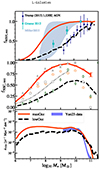 |
Fig. 9. Variations of the seeding probability in L-Galaxies BH. Top and middle panels: occupation fractions of MBH (M• > 105 M⊙, top) and NSC (all masses, middle) that result into the volumetric TDE rates as a function of galaxy-host mass (bottom). We show the maxOcc and lowOcc models with orange solid and black dashed lines, respectively. In the top panels we display the local MBH occupation fraction derived from a compilation of detections 2012 (2012, cyan squares) and X-ray constraints by Miller & Davies (2012, light-blue region), as well as an occupation for slightly higher redshifts 0.01 < z < 0.1 derived via optical-line AGN Trump et al. (2015, blue circles). In the middle panel, the data points and logistic function (the dashed-dotted thin line), both from Hoyer et al. (2021), have the same meaning as in Fig. 2. The enhanced MBH occupation is still compatible with the observations of the Coma Cluster (gray triangles), even though it yields a greater fraction of nucleated galaxies. We stress that all NSCs are hosting an MBH in our model, hence adding NSCs without MBHs would increase this fraction. Bottom panel: Both maxOcc and lowOcc model (solid and dashed line) reproduce the TDE-rate distribution constraint of Yao et al. (2023) within errors. However, in the lack of evidence of TDEs in dwarf galaxies the lowOcc model is preferred. |
The bottom panel of Fig. 9 shows that the changes in the MBH and NSC occupation result in appreciable differences in the observed TDE rates per galaxy. Although the maxOcc model also shows good agreement with the results of Yao et al. (2023) it lies on the upper limits of the observational constraints. Quantitatively, both of the models suggest: p ≲ −1 for  , instead of p ≳ 0, as found by Yao et al. 2023. Also, both the maxOcc and fiducial models support the interpretation of van Velzen (2018) for a flat (∼100%) occupation fraction of MBHs down to M* ∼ 1010 M⊙, while lowOcc model does not (see middle panel of Fig. 9). The noticable difference in the dwarf galaxy regime (M* = 107 − 1010 M⊙) is the main driver in boosting the volumetric TDEs at all galaxy stellar masses. Conversely, the fact that we do not detect TDEs at M* < 109 M⊙ may be primarily interpreted as a lower occupation fraction of MBHs than the one predicted by L-Galaxies BH, indicative of a less efficient seeding mechanism.
Regarding the NSC occupation, while the fiducial model (see Fig. 2) matches the observations of Virgo (and Fornax at lower masses) clusters (Muñoz et al. 2015; Eigenthaler et al. 2018; Sánchez-Janssen et al. 2019), the maxOcc resembles the higher NSC occupation in the Coma cluster (den Brok et al. 2014; Zanatta et al. 2021) and the lowOcc that of the Local Volume. Most of the clusters in our model are less massive than their MBH mass (see Appendix A for mass distribution of NSCs). In particular, only ≈30% and 60% of MBHs, hosted in galaxies with mass M* ∼ 107 M⊙ and 109.5 M⊙ at z = 0, are also found in an NSC more massive than them, namely 𝒟 = MNSC/M• > 1. For reference, the median mass ratio between NSCs and their associated MBHs with a measured mass is 𝒟 ∼ 4 (Greene et al. 2020), although detections are made in the most massive systems hosting MBHs M• > 106 M⊙.
We underline that there is a degeneracy between the occupation of MBHs per galaxy and the occupation of NSCs per MBH. In particular, simultaneous increase and decrease of each number density can result in the same observed normalization of the volumetric TDE rates. Interestingly, denser environments (galaxy clusters) are found to have higher-than-average occupation fractions of both MBHs (Tremmel et al. 2024) and NSCs (Sánchez-Janssen et al. 2019; Hoyer et al. 2021; Zanatta et al. 2021; Leaman & van de Ven 2022) at a given galaxy stellar mass, in line with maxOcc model predictions. Based on our model and the novel TDE rates per-galaxy of our study we speculate that the following conditions should be fulfilled by future models, for them to explain the observed TDE rates: (i) a tight connection between the two families of nuclear compact objects (in our model all NSCs host an MBH) and (ii) the dominant contributor to TDE rates to be MBHs hosted in M* ∼ 109 − 1010.5 M⊙ galaxies in dense environments, where NSC and MBH occupation reach 100% and the per-galaxy rate is peaking. An explicit study of the environment dependence, involving realistic star clusters and NSC modeling will be needed to further understand the connection between the two classes of objects.
4.3. Spin evolution and implications for tidal disruption event rates
Massive black holes close to the Hills mass (M• ∼ 108 M⊙) should exhibit near-to-zero TDEs by z = 0, and if they do they should be spinning (Kesden 2012). Also, because of their rarity, any TDE observed in this mass range will reside statistically at higher redshift (van Velzen 2018; Mummery & Balbus 2020; Hammerstein et al. 2023). Still, with the handful of massive systems observed with TDEs in the ZTF sample (Yao et al. 2023) we can test large volume statistics of the model’s MBH spin distribution.
As shown in Sect. 2.1, L-Galaxies BH predicts a median spin of χ• ≈ 0.75 for MBH with masses M• > 107 M⊙, with a standard deviation of σχ• ≈ 0.2. We note that when initially applied on the lower-resolution Millennium-I simulation (Izquierdo-Villalba et al. 2020), the spin model predicts that M• ≲ 108 M⊙ MBHs remain high-spinning (χ• > 0.8) down to z ∼ 0.1. Overall, the agreement19 of the shape of the predicted volumetric rates at high MBH masses with observations (Fig. 5) suggests that the model makes a reasonable prediction of the spin distribution at z < 0.5.
To guide the reader and bracket the effect of the spin model on the event horizon suppression, Fig. 10 displays the volumetric TDEs for the same MBH population of the fiducial model but assuming χ• = 0 and χ• = 0.998 when computing the event horizon suppression (Sect. 2.3.4) as a shaded region around the model line. As shown, a nonspinning MBH population in the mass range M• = 107.5 − 108.5 M⊙ (left border of the shaded region) can be excluded while a maximally spinning population in the same range, the model rates lie within the error margins of the constraints. Our results are consistent with the recent findings from Mummery et al. (2024) who derived MBH spin χ• = 0.3 − 0.75 by modeling the late-time TDE emission of 10 MBHs with mass M• > 107 M⊙.
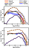 |
Fig. 10. Volumetric rates at z = 0 per black hole mass (top) and galaxy stellar mass (bottom) for different model variations (names of the models in legend as in text) compared with constraints from Yao et al. (2023, blue shaded area) and the fiducial model (red solid line). The orange shaded area was constructed by assuming no spin and maximally spinning MBHs in the post-processing treatment of the event horizon suppression of the fiducial model (orange solid line). |
We are careful with our interpretation since for converting simulated TDE rates to observable ones we have neglected some aspects of the disruption of the stars themselves. For example, we have used a truncated (m* < 1.5 M⊙) Kroupa IMF for the event-horizon suppression calculations. Nevertheless, the scenario of a top-heavy initial stellar mass functions for the stellar nuclear environment is frequently referenced as an alternative to high-spinning MBHs (Mockler et al. 2022). Our results may also be affected by the distribution of the stellar orbit inclinations as recently indicated by Singh & Kesden (2024). Furthermore, the effects of the De Sitter precession of the streams of the disrupted star on the outcome of a TDE may play an important role20 (stream self-crossing becomes ineffective Bonnerot et al. 2022; Jankovič et al. 2024, for reference). Nevertheless, our model suggests that basic assumptions for the star population and the detectability of individual events (Sect. 2.3.4), coupled with the spin distribution of L-Galaxies BH, can fairly reproduce the observed event horizon suppression.
4.4. The impact of parameter choice
As seen before, the occupation fraction of MBHs in galaxies seems to play an important role in the normalization of the volumetric TDEs, MBH spin distribution regulates the shape at the event horizon suppression. Here, we examine how TDE rates are influenced by other free parameters related to the NSC model (nucleation, regeneration, and compactness) and by the conditions used to reset the TDEs. We highlight that we do not seek to explore the full parameter space but rather pinpoint the most important choices for the model. Also, we stress that our main results for MBH growth do not change qualitatively among runs featuring single-parameter variations.
More compact nuclear star clusters. NSCs are the main stellar environments in which TDEs occur (compared to the galaxy contribution, see both per-galaxy and volumetric TDE rates in Figs. 6 and 7). When computing the number of TDEs of NSCs inside PHASEFLOW we assumed an effective radius of NSCs according to specific scaling relations (see Sect. 2.2). However, a large number of uncertainties are still present in these relations. For example, NSCs hosting an MBH are expected to dynamically evolve (evaporate/expand), so the observed scale radius may be greater than the initial radius (Merritt 2009). Therefore, we have also explored how the compactness of the NSC affects the number of TDEs and consequently, the volumetric TDE rates (hereafter the “compactNSC” model). In Fig. 10, we show the volumetric rates for a run where NSCs are initialized with a scale radius a reduced to 1/3 of what is assumed in our fiducial model (see Sect. 2.2.2). This choice is motivated by observations showing NSCs who lie ∼0.5 dex below the mass-radius relation for NSCs at z = 0 (see e.g. Pechetti et al. 2020). We observe that the model overpredicts the rates for MBH masses M• = 106 − 107.5 M⊙ by more than an order of magnitude. The overestimation disfavors NSCs that are significantly more compact than the observed relations used in our fiducial model. We stress that with the current implementation of NSCs, the model lacks the most massive NSCs of mass MNSC = 108 − 109 M⊙, which are naturally more compact and will contribute at TDE rates of M∙ > 107.5 M⊙ MBH.
Variation of 𝒟nuc. This is a key parameter in our model since it controls the frequency of NSC regeneration. Considering lower values than our fiducial case, observations presented in (Neumayer et al. 2020) suggest a value of 𝒟 ≡ MNSC/M• as low as 0.01. However, it remains unclear if these configurations are just transients. Despite that, we test a value of 0.01, and no significant changes are found. For the sake of brevity and clarity, we do not display the results of this run. Instead, we boost 𝒟nuc toward higher values, from 0.1 to 1 (hereafter the “Dnuc1” model) and show our results in Fig. 10. For this case, the rates are heavily suppressed at high MBH mass (M• > 107.5 M⊙) since the NSCs with values 𝒟nuc = 0.1 − 1 are not nucleated in this run. This is a piece of evidence that small and possibly unresolved NSCs (𝒟 < 1) are the main contributors to TDE rates in the event-horizon suppression mass range. However, only the replacement of this parameter with a physical NSC treatment (including the destruction of NSCs) can offer hindsight on why this is the case.
Variation of cutoff galaxy stellar mass for nucleation. Recently, the careful observational sampling of massive galaxies presented in Ashok et al. (2023) finds a possible higher nucleation fraction in the high-mass end than the one reported in the observational constraints used for this work (i.e. Hoyer et al. 2021). In our phenomenological model of NSCs, we impose a maximum galaxy stellar mass M*, NSC-cutoff = 109.75 M⊙ (Sect. 2.1.4), above which either the conditions are not adequate to trigger the NSC formation or, equivalently, the destruction of NSC becomes important. The specific value of this cutoff is extremely important for M* > 1011 M⊙ galaxies since higher values of the cutoff allow for not only a higher number density of NSCs but also more massive NSCs (since the scaling relation extends to high-mass galaxies). On the other hand, a sufficiently low M*, NSC-cutoff can turn off the nucleation around M• > 108 M⊙ MBHs, converting the galaxy component to the only source of TDEs in this mass range.
To explore how the volumetric rates are affected by the nucleation mass cutoff, in Fig. 10 we present the results of a run where no cutoff has been applied, that is, all galaxies at all masses can host an NSC as long as 𝒟nuc > 0.1 (hereafter the “noMstcut” model). As compared to the fiducial model, this parameter variation shows that the inclusion of more massive clusters at more massive galaxies will not affect the low-mass regime of the volumetric rate distribution and increase the rates at the event horizon suppression with error margins. These “more massive” NSCs can be similarly introduced by increasing the scatter on the M* − MNSC scaling relation when assigning NSC masses in the model. We anticipate the inclusion of a realistic scenario for NSC evolution and destruction will increase the TDE rates in massive galaxies.
Variation of tidal disruption event rates reset frequency. To assess the importance of the conditions used to reset the TDE rates (see Sect. 2.3.2) we consider that only major events are capable of resetting the clock of TDEs (ΔtTD, i). In particular, major events refer here to (i) major galaxy mergers (satellite/central baryonic mass ratio > 10%) and (ii) disk instability events that displace more than > 10% of the stellar disk mass to the bulge. Hereafter, we refer to this model as OnlyMajor and we present its volumetric TDE rates in Fig. 10. Overall, the predictions of the model are ∼1 dex below the current observational constraints regardless of the MBH and galaxy stellar masses. Yet, the suppression of rates induced by the OnlyMajor model for galaxies with M* ∼ 1011 M⊙ leads to a better agreement with observations than for the fiducial model. This points out that minor events occurring in massive galaxies should take place away from the galactic nucleus, hindering their possibility of resetting the TDE rates. While this might be true for massive systems, it is unlikely that for small galaxies catastrophic events such as major mergers or important disk instabilities are the unique processes able to significantly modify the stellar environment around nuclear MBHs and thus reset the relaxation process.
The underprediction of the volumetric TDE rates for small MBHs and galaxies shown in OnlyMajor model highlights that NSC structures (that dominate the overall TDE rates, see Sect. 3.1) should be dynamically influenced by their host galaxy interactions quite often. For instance, the accretion of nonmajor satellites and weak disk instabilities should result in a relatively frequent refilling of the loss cone of their hosted MBH. An important caveat to this argument is that catastrophic events are the type of interactions in which the basic assumptions of spherical symmetry and isotropy of stellar profiles (assumed in this work) are most frequently violated and a rate enhancement may occur (see Sect. 5).
5. Limitations and prospects
In this section, we discuss the main limitations that cannot be addressed with our methods. In addition, we discuss further details on the nature of TDE events that could potentially be captured in the framework of our model. We make some suggestions for improvements regarding both the use of PHASEFLOW and L-Galaxies, as well as motivate further research projects as an extension to this work.
5.1. Caveats regarding input tidal disruption event rates
As pointed out in Merritt (2013), the 1D Fokker Planck approach (see Sect. 2.2) may be inaccurate over the relaxation timescale. A more general treatment that accounts for the evolution of energy and angular momentum may be reliable on longer timescales, over which the angular momentum profile alters the overall evolution of the stellar profile (see e.g. Broggi et al. 2022). Moreover, there are effects that cannot be taken into account in PHASEFLOW, at least in its current form. Noticeable ones are: resonant relaxation of Keplerian orbits (Rauch & Tremaine 1996), large scattering (instead of diffusing into the loss-cone Weissbein & Sari 2017) or loss-cone shielding (Teboul et al. 2024); all of which have been shown to have an impact on TDE rates for specific systems. On top of this, relativistic effects may affect the outcome of the interactions and thus the prediction of the rate (e.g. Stone et al. 2019). Addressing all these caveats would require a different solution to the problem than the one provided with two-body energy relaxation as performed by PHASEFLOW.
In addition to the limitations due to the negligence of anisotropies, the current method is limited to working with spherical systems (while many systems are observed rotating and therefore flattened). Although Merritt (2013) argues that nonaxisymmetry affects rate estimation within a factor of two, we stress that rates for axisymmetric profiles have been noted to deviate from the ones produced with PHASEFLOW (see e.g. Vasiliev & Merritt 2013). Kim et al. (2018) find evidence of elongated bulges being correlated with nuclear starbursts21, which may be a possible way to allow an increase in rates for a specific type of bulge. The bursty behavior of high TDE rates in certain galaxy types has been explained through radial anisotropies (Stone et al. 2018), occurring through the formation of eccentric disks (Madigan et al. 2018; Rantala & Naab 2024), as opposed to overdensity in the nucleus (as assumed in this work). Nevertheless, it is worth noticing that observations have been favoring the latter (French et al. 2020a). All these are subjects that have mainly been explored by expensive N-body simulations with tailored initial conditions and go far beyond the general/average viewpoint we have drawn for the global TDE rates.
The stellar initial mass function is also an important caveat to expand on. All systems (young and old) are assigned TDE rates from an evolved population of stars, represented by the average of the Kroupa mass function, and heavy black holes. The particle mass and the fraction of total mass of this heavy component (16 M⊙ at 7% of the cluster’s mass respectively) drive the magnitude of mass segregation in energy (a process that has its own timescale and may damp the rates, see Bortolas 2022). Since the initial phase is affected by mass segregation and low-mass systems clusters during the initial phase have higher per-galaxy TDE rates (see Fig. 6), the choice of these parameters should be investigated further in the future when studying the growth and the rates at these systems.
Regarding the complexity of the initial mass function, the theoretical calculation of rates only demands the first two moments of mass (see Stone & Metzger 2016). Therefore, we expect that a more complete mass distribution will not impact severely the total number of events (but only a factor of a few). Moreover, in our model, the NSC profiles are motivated by the assembly of NSCs through the accumulation of globular clusters (Antonini et al. 2012), which will have themselves evolved stellar populations (see recent advancement in simulations of the formation of NSCs by Gray et al. 2024). However, for clusters that form for the first time in a galaxy at high redshift, the assumed actual initial mass function could be lacking stellar black holes that need some time to form as remnants of the first massive stars, but also it could be more top-heavy than is currently assumed (Chon et al. 2021; Sneppen et al. 2022; Cameron et al. 2024). Going beyond the bi-chromatic distribution into a realistic initial mass function is limited for now from the computational feasibility of a huge parameter space for the input tables22.
5.2. Caveats regarding the galaxy environment
Regarding the galaxy evolution model used in this work, one of the main aspects affecting the TDE demographics is the galaxy sizes predicted by L-Galaxies BH (initially introduced by Guo et al. 2011). Despite being traced self-consistently the expected sizes do not capture some particular galaxy classes discovered in the last decade (e.g. ultra-compact dwarfs). The inclusion of more refined environmental effects included in other L-Galaxies versions (e.g. Ayromlou et al. 2021, that adds ram-pressure stripping), may be necessary to capture the nature of these types of objects.
Regarding galaxy profiles, there are also some improvements in the modeling of stellar dynamics that can be included in our semianalytical approach. Specifically, the Sérsic indices assigned to bulges by L-Galaxies BH are motivated by z = 0 observations. However, this does not take into account the evolutionary history of galaxies. For instance, systems in a post-starburst and early quiescent phase (Setton et al. 2022), as well as “red nuggets” (e.g. Saracco et al. 2010; Barro et al. 2013; Ito et al. 2024; Baggen et al. 2023; Lohmann et al. 2023; Pandya et al. 2024), have been shown to display a larger Sérsic index than ordinary galaxies. Finally, the bulge velocity dispersion is not included self-consistently in L-Galaxies BH. This hinders the possibility of exploring the effect of this quantity on the TDE rates. For instance, observations of “σ-drop” bulges (Comerón et al. 2008) suggest that some bulges will have a low enough velocity dispersion to significantly shorten relaxation timescales and thus change the expected TDEs (Cen 2020).
Regarding the reset mechanism (Sect. 2.3.2), internal processes such as phase-mixing, gravitational heating from perturbers (e.g., giant molecular clouds, Merritt 2013), and bar interactions with the nuclear region will certainly affect the event rates. These effects cannot be captured by our model since they are not quantified in L-Galaxies BH but rather would require modeling through expensive, dedicated hydrodynamical simulations that also include TDEs.
Finally, regarding the NSC phenomenological scheme itself, we do not explore nor the redshift-dependence of the scaling relations neither the conditions under which a galaxy will host an NSC. For example, NSCs can both lose mass over time due to stellar evolution, two-body relaxation, tidal shocks and MBH interactions and gain mass through in situ star formation or cluster mergers. This makes uncertain the evolution of the NSC–galaxy stellar mass scaling relation in Eq. (1). If we assume that, at higher redshifts and in dwarf galaxies, NSCs were more massive and more compact than the observed values at z ∼ 0, the TDE rates will increase accordingly and could result in a disagreement with the observational constraints. Conversely, suppose we assume that most high-mass NSCs in the present-day Universe accumulated their mass over time via in situ star formation. In that case, they might have been lower-mass at higher redshift compared to today, which would result in lower high-redshift TDE rates (causing a stronger redshift-dependence in Fig. 7) and could contribute to the overprediction of TDE rates in massive galaxies (right panel of Fig. 5).
5.3. Rate enhancement
The highest per-galaxy rate predicted by our fiducial model corresponds to ∼10−4 yr−1, compatible with the earliest results of Syer & Ulmer (1999). Despite that, a sample of galaxies like ULIRGs or E + A(k + a) post-starbursts seem to feature rates of 10−3–10−1 per year, values that are not reproduced in any individual galaxy of L-Galaxies BH, and rarely occur in the input grid of TDE rates (see Sect. 2.2.2). The large rate seen in post-starburst galaxies could be the result of a TDE enhancement driven by particular conditions. For instance, the recent theoretical work of French et al. (2017) supports the amplification of TDEs in the core of post-starburst galaxies, driven primarily by the compactness of these systems and not by the initial stellar mass function variations (Bortolas 2022). Another interpretation is that as soon as the AGN phase is over, the loss cone region around the MBH can be filled, thus boosting the expected TDE rates by up to two orders of magnitude compared to standard nuclei (Wang et al. 2024). Moreover, a significant fraction of MBHs in L-Galaxies BH are found in binaries (in MS by z = 0 galaxies with M* = 1010 − 1011 M⊙ host MBH binaries with primary’s mass M• > 107 M⊙, see Fig. 8 in Izquierdo-Villalba et al. 2023) at which the rates of the secondary MBH can be enhanced to be similar to those of the most massive one (see Li et al. 2017; Ryu et al. 2022; Mockler et al. 2023, and discussion further below). There are therefore three plausible explanations for the scarce number of cases with TDEs rates per MBH as high as > 10−4 yr−1 in our model23: (i) the stellar profile of dwarf and intermediate-mass galaxies is not correctly captured at all times, (ii) at least one enhancement mechanism due to additional physics is determining the global rates and should be included, or (iii) the theoretical uncertainty regarding the initial NSC profiles and the accuracy of the initial relaxation phase hinders the possibility of probing the initial prompt phase of violent relaxation for these objects. To examine the last explanation, a cautious approach for the initial “bursty” phase when resetting the stellar environment around the MBH (see Sects. 2.2 and 2.3.2) may resolve this problem. This will be the subject of exploration in future work.
If the rates in the aforementioned over-represented classes of galaxies are indeed dominated by NSC rates, a more careful treatment of NSCs at different galaxy types could yield exceptionally high rates. Denser, cuspier, and more massive clusters are all conditions that have a non-negligible impact on the evolution of time-dependent TDE rates (Broggi et al. 2022). We have already noted that the introduced phenomenological model does not produce the most massive NSCs of mass MNSC = 108 − 109 M⊙ (see the mass function in Appendix A). In addition to that, the formation channel via accretion of clusters (assumed in this work) appears to operate in dwarf galaxies (MNSC < 108 − 109 M⊙, Johnston et al. 2020; Fahrion et al. 2021, 2022); yet central star formation may dominate cluster formation in larger galaxies (Aharon & Perets 2015; van Donkelaar et al. 2024). Consequently, the spheroidal profile used for this work could not be applied in such cases (see also Kacharov et al. 2018 and Pinna et al. 2021 for differences with host galaxy morphology). However, for the inclusion of cuspier profiles, mass segregation in angular momentum – which cannot be captured by PHASEFLOW – will prevent the model from correctly computing the TDE rates, and a more sophisticated approach may be needed.
5.4. Other classes of star-massive black hole interactions:
In this work, we have focused our results on the rates of full TDEs and their contribution to MBH growth. However, there are many possible directions for future work exploring physically different types of interactions between stars and MBHs.
5.4.1. Partial tidal disruption events
Partial tidal disruption events (partial TDEs) might be equally important for the growth of black holes as full TDEs. For example, Zhong et al. (2022) find that partial TDEs are super-Eddington 2.5 times more frequently than full TDEs, while the repetitive nature of these events can spoon-feed the MBH with increased efficiency MacLeod et al. (2012), Ryu et al. (2020b). Partial TDE rates are as high as those of full disruptions both theoretically (Krolik et al. 2020) and from recent observations (Somalwar et al. 2023b). Recently, Bortolas et al. (2023) by tracing the fate of the remnants of such events and the inferred rates using PHASEFLOW showed that partial TDEs can be more frequent than full TDEs up to a few tens of times for nucleated galaxies. However, the radiative signatures of partial TDEs, and how they compare with those of full TDEs, need to be addressed before discussing further their statistics (e.g., a TDE can be falsely attributed as a rising AGN event, see e.g. Chen & Shen 2021). If indeed partial outnumber full TDEs, the volumetric TDE rates may be even lower, possibly indicating a model-observation tension toward the low-mass regime (M• < 106 M⊙). One of the dimmest events of Yao et al. (2023), AT2020vdq with an assigned mass of M• ∼ 105.5 M⊙, has recently been flagged as a partial disruption (Somalwar et al. 2023a), a class of events that is not included in our predictions. If these and other events at M• < 106 M⊙ are indeed partial disruptions that would mean a tension between our model and observations (in Fig. 5). We continue this discussion quantitatively in Appendix B for the interested readers, where we introduce some relevant definitions.
In general, different orbit distributions will result in different frequencies of full TDEs, partial TDEs, and direct captures (Park & Hayasaki 2020; Cufari et al. 2022), but also different rates for certain subcategories of full TDEs, for example, relativistic TDEs (Ryu et al. 2023; Amaro Seoane 2024) and TDEs with eccentric debris disks (Zanazzi & Ogilvie 2020; Wevers et al. 2022). Tapping into the statistics of the orbits can serve as an additional time-dependent output in the grid-like exploration of the parameter space, which can then be provided as L-Galaxies input, addressing the aforementioned issues. We plan to improve this aspect of the model in future works.
5.4.2. Rates from binary and wandering massive black holes
The rich physics shaping the evolution of two (or more) MBHs toward coalescence following galaxy mergers, may significantly affect TDE rates. In the pairing phase, MBHs move within the potential of the bulge (not lying anymore in the dense center) and produce different rates of TDEs than central MBHs, with possible enhancement of rates during passages of stellar overdensities (Merritt 2013). After the formation of a binary (on parsec scales), the eccentric Kozai-Lidov mechanism can boost the rates of the secondary MBH to be similar to the most massive one (Chen et al. 2011; Mockler et al. 2023). Also at smaller separations (a multiple of the sum of the two MBHs tidal radii), the rates are theoretically expected to be boosted (Li et al. 2017; Ryu et al. 2022). An important enhancement would allow for an indirect inference of binaries through TDEs (Mockler et al. 2023), something to be investigated in follow-up work dedicated to rates from binary MBHs.
Finally, the inclusion of wandering MBHs, assuming that a significant amount of them can maintain a massive star cluster after ejection, may contribute to the overall TDE signal and add to the off-nucleus signal from MBHs in globular clusters (expected to be lower than the nuclear MBHs Ramirez-Ruiz & Rosswog 2009), especially when considering the smallest MBHs. The inclusion of such rates could lead to a possible explanation of the nondetection of a host galaxy (e.g., the long-duration TDE “scary barbie” Subrayan et al. 2023) or other off-nuclear transients (e.g., the Fast Blue Optical Transient “Finch” Chrimes et al. 2024).
5.4.3. Electromagnetically dark events
Extreme Mass Ratio Inspirals (EMRIs) and Direct Plunges (as defined in Broggi et al. 2022) of stellar remnants have their own evolution within an NSC. Given the relatively large mass accreted for each EMRI and plunge event, MBH growth via dark accretion of compact objects might even be more important than accretion through TDEs. However, while the distribution of stars in NSCs can be constrained by observations, there is no direct way to probe the distribution of nonluminous objects24. This adds large theoretical uncertainties in calculating the cosmological rates. Also, regimes where general relativity effects are dominant over two-body relaxation should be taken into consideration.
Also of great interest, binary stars have a large tidal radius (Merritt 2013, 10–100 times that of a single star), while a binary system may be disrupted consecutively, either by one or both MBHs (Wu & Yuan 2018). For realistic EMRI and plunge rates, triple interactions between stellar remnant binaries and the MBH must be considered (Bonetti et al. 2019; Bonetti & Sesana 2020). Our method is currently not ideal for the inclusion of binary stars and remnants. We aim to investigate the aforementioned type of interactions, along with their contribution to the gravitational wave background to be probed by Laser Interferometry Space Antenna (LISA), in a future dedicated study.
6. Conclusions
In this work, we have included for the very first time TDEs from MBHs in a semianalytic model of galaxy formation and evolution. To this end, we have used the L-Galaxies model (Henriques et al. 2015) in the version presented in Izquierdo-Villalba et al. (2020, 2022) and Spinoso et al. (2023), which includes many physical processes that drive the formation and evolution of MBHs. For this work, we also included a phenomenological model for NSCs that uses the observed NSC-galaxy stellar mass relations and reproduces the observed NSC occupation fraction. Time-dependent TDE rates for each galaxy were then obtained by solving the 1D Fokker-Planck equation with PHASEFLOW for a variety of stellar environments surrounding the MBHs. Finally, we made simple post-processing assumptions in order to transform the theoretical rates to observable rates. The key findings of the model are summarized in the following:
-
Our model predicts volumetric TDE rates that are in agreement with the observed ones. Rates from the disruptions of stars belonging to the stellar disk or bulges alone cannot explain the observations. Instead, we predict that the majority of TDEs should take place in NSCs, independently of galaxy or black hole mass. To explain the rates within the local cosmological volume (z < 0.5), a steep black hole mass function (
 at M• ∼ 105 − 106.5 M⊙) and a relatively high occupation fraction of black holes also in the dwarf regime are needed.
 -
The TDE rates per-MBH do not follow a single power law as obtained in other works from scaling relations (e.g.,
 with −0.4 < B < 0, see Wang & Merritt 2004; Stone & Metzger 2016; Pfister et al. 2020). Instead, our model produces a positive power-law dependence, with B ≈ 0.7 for the TDE rates from the galaxy component that peak at M• = 108 M⊙, before the event horizon suppression completely takes over. For the rates from the NSC component (which dominate the total rates), we predict a power-law index of B = 0 and B = 1 for young and old NSCs, respectively, turning over at M• ∼ 107 M⊙.
 -
The spin distribution, a result of the MBH spin model introduced in L-Galaxies BH by Izquierdo-Villalba et al. (2019) naturally explains the event horizon suppression observed in the optical TDE samples. The model points out that MBHs of mass M• = 107 − 108.5 M⊙ have a median spin of
 with a standard deviation of σχ• ≈ 0.2.
 -
A great fraction of the TDEs (∼100% for the most massive hosts M* > 1011 M⊙) takes place around MBHs that are also experiencing some level of gas accretion. We thus predict TDEs to be detectable on top of low-luminosity AGN (bolometric luminosity 3 × 1040–1042 erg/s), although AGN are generally excluded from TDE searches. Also, we predict TDE-like flares to have a volumetric rate of 0.3 − 1 Gpc−3 yr−1 dex−1 for Seyfert galaxies with AGN luminosity Lbol = 1042-1045 erg/s in the broad mass range M* = 108 − 1010.5 M⊙, with the rate increasing by a factor of a few tens at redshifts z ≥ 1.
To conclude, the model presented here, a combination of L-Galaxies BH and PHASEFLOW, can overall reproduce the latest observed TDE rates while respecting the constraints on the galaxy and black hole mass functions. Our results highlight the importance of using a realistic cosmological framework to obtain a comprehensive view of TDE demographics. Furthermore, our results underline the importance of including time-dependent TDE rates (as demonstrated in Broggi et al. 2022), which allow for accounting of the relaxation timescale in the statistics, unlike studies that use instantaneous TDE rates.
Finally, while we did not find a significant contribution of TDEs to the average MBH mass growth, TDE growth might be important for specific classes of MBHs and seeds; this will be investigated in a follow-up work (Polkas et al., in prep.). We also plan to address the caveats and limitations of our model in future works in order to improve its ability to draw predictions for TDEs and the associated growth of MBHs, particularly in view of the upcoming flow of data from LSST.
In the occurring field of TDEs from stellar mass black holes (Kremer et al. 2022, 2023; Vynatheya et al. 2024; Xin et al. 2024), the events are frequently referred to as micro-TDEs, so we preserve the term “TDE” for events from massive black holes.
The Lyman-Werner (LW) band is a specific energy-interval (i.e., hν = [11.2 − 13.6] eV) in the UV spectrum. LW photons are responsible for the photo-dissociation of molecular hydrogen (e.g. Haiman et al. 1997).
We noted the existence of a few nearby galaxies hosting an NSC but lacking an SMBH: M 33 (Gebhardt et al. 2001; Merritt et al. 2001), M 110 (Valluri et al. 2005), or NGC 7793 (Neumayer & Walcher 2012).
The choice for these values for the mass of main sequence stars and stellar black holes comes from the fact that those are close to the average masses for those objects assuming an evolved Kroupa (2001) stellar mass function; in addition, the second moment of the mass function, which sets the relaxation rate of the system and thus the TDE rates, attains a value which is very close to the actual one if we were to assume a complete and evolved stellar mass function (see e.g. Kochanek 2016; Stone & Metzger 2016; Pfister et al. 2022; Bortolas 2022).
At a full disruption, the MBH captures 50% of the stellar mass. We selected a subsequent mass loss due to radiation and winds removing 40% of the bound material based on results from observations (Mockler & Ramirez-Ruiz 2021) and simulations (Bu et al. 2023). Simulations including radiative transfer from Steinberg & Stone (2024) yield a lower percentage of 15%.
From theory (e.g., MacLeod et al. 2012 and Kochanek 2016), for a given M•, TDE rates scale with the initial mass function dN/dm* and power law  . This will matter mostly beyond the maximum Hills mass for m* = 0.38 M⊙ (M• > 108 M⊙), a mass range that TDE rates are shown only indicatively. Although the dependence on the initial mass function is captured with the sampling of stars, we did not rescale rates with this power-law dependence for massive monochromatic stars when adding them to the bulk rates.
For the sake of brevity, we do not show the black hole mass function of the maxOcc model. This model tends to overpredict by a factor of three the number of MBHs in the mass range M• = 106 − 107.5 M⊙, compared to observational constraints at z = 0 from Shankar et al. (2009). Besides this, the overall shape of the mass function remains relatively similar concerning the fiducial model at high masses.
We stress that we have identified the slight underprediction to be due to the lack of massive NSC abundance by the model as discussed in our results (see Sect. 4.4, model tagged as noMstcut).
This refers to both convection-dominated and radiation-dominated stars since the fraction of full TDE rates is already is over-estimated by a factor of (βc)Sβ when assuming the TDE rates of 0.38 M⊙ stars hold for more massive stars PHASEFLOW. Also, the weak dependence of βc on MBH mass in the regime is neglected.
Acknowledgments
This work used, as a foundation, the 2015 public version of the Munich model of galaxy formation and evolution: L-Galaxies. The source code and a full description of the model are available at https://lgalaxiespublicrelease.github.io/. It also uses the publically available 1D-Fokker Planck solver PHASEFLOW available at http://eugvas.net/software/phaseflow/. We thank Rosa Valiante for kindly allowing us to use her catalogs of GQd for the PopIII sub-grid physics. M.P. and S.B. acknowledge support from the Spanish Ministerio de Ciencia e Innovación through project PID2021-124243NB-C21. A.S., D.I.V. and E.B. acknowledge the financial support provided under the European Union’s H2020 ERC Consolidator Grant “Binary Massive Black Hole Astrophysics” (B Massive, Grant Agreement: 818691). E.B. acknowledges support from the European Union’s Horizon Europe programme under the Marie Skłodowska-Curie grant agreement No 101105915 (TESIFA), from the European Consortium for Astroparticle Theory in the form of an Exchange Travel Grant, and the European Union’s Horizon 2020 Programme under the AHEAD2020 project (grant agreement 871158). N.H. is a fellow of the International Max Planck Research School for Astronomy and Cosmic Physics at the University of Heidelberg (IMPRS-HD). N.H. received financial support from the European Union’s HORIZON-MSCA-2021-SE-01 Research and Innovation programme under the Marie Sklodowska-Curie grant agreement number 101086388 – Project acronym: LACEGAL. D.S. acknowledges the support of the National Key R&D Program of China (grant no. 2018YFA0404503), the National Science Foundation of China (grant no. 12073014), the science research grants from the China Manned Space Project with No. CMS-CSST2021-A05, and Tsinghua University Initiative Scientific Research Program (No. 20223080023).
References
- Aharon, D., & Perets, H. B. 2015, ApJ, 799, 185 [NASA ADS] [CrossRef] [Google Scholar]
- Alexander, T., & Bar-Or, B. 2017, Nat. Astron., 1, 0147 [NASA ADS] [CrossRef] [Google Scholar]
- Amaro Seoane, P. 2024, MNRAS, submitted [arXiv:2307.13043] [Google Scholar]
- Angulo, R. E., & White, S. D. M. 2010, MNRAS, 405, 143 [NASA ADS] [Google Scholar]
- Antonini, F., Barausse, E., & Silk, J. 2015, ApJ, 812, 72 [Google Scholar]
- Antonini, F., Capuzzo-Dolcetta, R., Mastrobuono-Battisti, A., & Merritt, D. 2012, ApJ, 750, 111 [NASA ADS] [CrossRef] [Google Scholar]
- Arca-Sedda, M. 2016, MNRAS, 455, 35 [NASA ADS] [CrossRef] [Google Scholar]
- Arca-Sedda, M., & Capuzzo-Dolcetta, R. 2014, MNRAS, 444, 3738 [NASA ADS] [CrossRef] [Google Scholar]
- Arcavi, I., Gal-Yam, A., Sullivan, M., et al. 2014, ApJ, 793, 38 [Google Scholar]
- Ashok, A., Seth, A., Erwin, P., et al. 2023, ApJ, 958, 100 [NASA ADS] [CrossRef] [Google Scholar]
- Askar, A., Davies, M. B., & Church, R. P. 2022, MNRAS, 511, 2631 [NASA ADS] [CrossRef] [Google Scholar]
- Atallah, D., Trani, A. A., Kremer, K., et al. 2023, MNRAS, 523, 4227 [NASA ADS] [CrossRef] [Google Scholar]
- Auchettl, K., Guillochon, J., & Ramirez-Ruiz, E. 2017, ApJ, 838, 149 [Google Scholar]
- Aversa, R., Lapi, A., de Zotti, G., Shankar, F., & Danese, L. 2015, ApJ, 810, 74 [NASA ADS] [CrossRef] [Google Scholar]
- Ayromlou, M., Kauffmann, G., Yates, R. M., Nelson, D., & White, S. D. M. 2021, MNRAS, 505, 492 [NASA ADS] [CrossRef] [Google Scholar]
- Bade, N., Komossa, S., & Dahlem, M. 1996, A&A, 309, L35 [NASA ADS] [Google Scholar]
- Baggen, J. F. W., van Dokkum, P., Labbé, I., et al. 2023, ApJ, 955, L12 [NASA ADS] [CrossRef] [Google Scholar]
- Bahcall, J. N., & Wolf, R. A. 1976, ApJ, 209, 214 [NASA ADS] [CrossRef] [Google Scholar]
- Baldry, I. K., Glazebrook, K., & Driver, S. P. 2008, MNRAS, 388, 945 [NASA ADS] [Google Scholar]
- Barro, G., Faber, S. M., Pérez-González, P. G., et al. 2013, ApJ, 765, 104 [Google Scholar]
- Bassino, L. P., Muzzio, J. C., & Rabolli, M. 1994, ApJ, 431, 634 [NASA ADS] [CrossRef] [Google Scholar]
- Begelman, M. C., Blandford, R. D., & Rees, M. J. 1980, Nature, 287, 307 [Google Scholar]
- Binney, J., & Tremaine, S. 1987, Galactic Dynamics (Princeton: Princeton University Press) [Google Scholar]
- Binney, J., & Tremaine, S. 2008, Galactic Dynamics, 2nd edn. (Princeton: Princeton University Press) [Google Scholar]
- Blanchard, P. K., Nicholl, M., Berger, E., et al. 2017, ApJ, 843, 106 [Google Scholar]
- Bonetti, M., & Sesana, A. 2020, Phys. Rev. D, 102, 103023 [NASA ADS] [CrossRef] [Google Scholar]
- Bonetti, M., Haardt, F., Sesana, A., & Barausse, E. 2018, MNRAS, 477, 3910 [Google Scholar]
- Bonetti, M., Sesana, A., Haardt, F., Barausse, E., & Colpi, M. 2019, MNRAS, 486, 4044 [NASA ADS] [CrossRef] [Google Scholar]
- Bonnerot, C., Pessah, M. E., & Lu, W. 2022, ApJ, 931, L6 [NASA ADS] [CrossRef] [Google Scholar]
- Bonoli, S., Marulli, F., Springel, V., et al. 2009, MNRAS, 396, 423 [NASA ADS] [CrossRef] [Google Scholar]
- Bortolas, E. 2022, MNRAS, 511, 2885 [NASA ADS] [CrossRef] [Google Scholar]
- Bortolas, E., Ryu, T., Broggi, L., & Sesana, A. 2023, MNRAS, 524, 3026 [NASA ADS] [CrossRef] [Google Scholar]
- Boylan-Kolchin, M., Springel, V., White, S. D. M., Jenkins, A., & Lemson, G. 2009, MNRAS, 398, 1150 [Google Scholar]
- Bricman, K., & Gomboc, A. 2020, ApJ, 890, 73 [NASA ADS] [CrossRef] [Google Scholar]
- Brockamp, M., Baumgardt, H., & Kroupa, P. 2011, MNRAS, 418, 1308 [CrossRef] [Google Scholar]
- Broggi, L., Bortolas, E., Bonetti, M., Sesana, A., & Dotti, M. 2022, MNRAS, 514, 3270 [NASA ADS] [CrossRef] [Google Scholar]
- Bu, D.-F., Chen, L., Mou, G., Qiao, E., & Yang, X.-H. 2023, MNRAS, 521, 4180 [NASA ADS] [CrossRef] [Google Scholar]
- Bučar Bricman, K., van Velzen, S., Nicholl, M., & Gomboc, A. 2023, ApJS, 268, 13 [CrossRef] [Google Scholar]
- Bykov, S.D., Gilfanov, M.R., & Sunyaev, R.A. 2024, MNRAS, submitted [arXiv:2310.00303] [Google Scholar]
- Cameron, A.J., Katz, H., Witten, C., et al. 2024, MNRAS, submitted [arXiv:2311.02051] [Google Scholar]
- Cannizzaro, G., Levan, A. J., van Velzen, S., & Brown, G. 2022, MNRAS, 516, 529 [NASA ADS] [CrossRef] [Google Scholar]
- Cao, X. 2010, ApJ, 725, 388 [NASA ADS] [CrossRef] [Google Scholar]
- Cao, X., You, B., & Wei, X. 2023, MNRAS, 526, 2331 [NASA ADS] [CrossRef] [Google Scholar]
- Capuzzo-Dolcetta, R. 1993, ApJ, 415, 616 [NASA ADS] [CrossRef] [Google Scholar]
- Carlsten, S. G., Greene, J. E., Beaton, R. L., & Greco, J. P. 2022, ApJ, 927, 44 [NASA ADS] [CrossRef] [Google Scholar]
- Carter, B., & Luminet, J. P. 1982, Nature, 296, 211 [NASA ADS] [CrossRef] [Google Scholar]
- Cen, R. 2020, ApJ, 888, L14 [NASA ADS] [CrossRef] [Google Scholar]
- Cenko, S. B., Bloom, J. S., Kulkarni, S. R., et al. 2012, MNRAS, 420, 2684 [NASA ADS] [CrossRef] [Google Scholar]
- Chan, C.-H., Piran, T., Krolik, J. H., & Saban, D. 2019, ApJ, 881, 113 [Google Scholar]
- Chandrasekhar, S. 1942, Principles of Stellar Dynamics (Chicago: The University of Chicago press) [Google Scholar]
- Charalampopoulos, P., Kotak, R., Wevers, T., et al. 2024, A&A, in press https://doi.org/10.1051/0004-6361/202449296 [NASA ADS] [CrossRef] [EDP Sciences] [Google Scholar]
- Chen, J.-H., & Shen, R.-F. 2021, ApJ, 914, 69 [NASA ADS] [CrossRef] [Google Scholar]
- Chen, X., Sesana, A., Madau, P., & Liu, F. K. 2011, ApJ, 729, 13 [NASA ADS] [CrossRef] [Google Scholar]
- Chon, S., Omukai, K., & Schneider, R. 2021, MNRAS, 508, 4175 [NASA ADS] [CrossRef] [Google Scholar]
- Chornock, R., Berger, E., Gezari, S., et al. 2014, ApJ, 780, 44 [Google Scholar]
- Chrimes, A. A., Jonker, P. G., Levan, A. J., et al. 2024, MNRAS, 527, L47 [Google Scholar]
- Cohn, H., & Kulsrud, R. M. 1978, ApJ, 226, 1087 [NASA ADS] [CrossRef] [Google Scholar]
- Comerón, S., Knapen, J. H., & Beckman, J. E. 2008, A&A, 485, 695 [NASA ADS] [CrossRef] [EDP Sciences] [Google Scholar]
- Coughlin, E. R., & Nixon, C. J. 2022, ApJ, 936, 70 [NASA ADS] [CrossRef] [Google Scholar]
- Croton, D. J., Springel, V., White, S. D. M., et al. 2006, MNRAS, 365, 11 [Google Scholar]
- Cufari, M., Coughlin, E. R., & Nixon, C. J. 2022, ApJ, 924, 34 [NASA ADS] [CrossRef] [Google Scholar]
- Dai, L., McKinney, J. C., & Miller, M. C. 2015, ApJ, 812, L39 [NASA ADS] [CrossRef] [Google Scholar]
- Davis, B. L., Graham, A. W., & Cameron, E. 2019, ApJ, 873, 85 [NASA ADS] [CrossRef] [Google Scholar]
- den Brok, M., Peletier, R. F., Seth, A., et al. 2014, MNRAS, 445, 2385 [NASA ADS] [CrossRef] [Google Scholar]
- Dgany, Y., Arcavi, I., Makrygianni, L., Pellegrino, C., & Howell, D. A. 2023, ApJ, 957, 57 [NASA ADS] [CrossRef] [Google Scholar]
- Dodd, S. A., Law-Smith, J. A. P., Auchettl, K., Ramirez-Ruiz, E., & Foley, R. J. 2021, ApJ, 907, L21 [CrossRef] [Google Scholar]
- Donley, J. L., Brandt, W. N., Eracleous, M., & Boller, T. 2002, AJ, 124, 1308 [NASA ADS] [CrossRef] [Google Scholar]
- Dotti, M., Merloni, A., & Montuori, C. 2015, MNRAS, 448, 3603 [NASA ADS] [CrossRef] [Google Scholar]
- Duffell, P. C., D’Orazio, D., Derdzinski, A., et al. 2020, ApJ, 901, 25 [NASA ADS] [CrossRef] [Google Scholar]
- Efstathiou, G., Lake, G., & Negroponte, J. 1982, MNRAS, 199, 1069 [NASA ADS] [CrossRef] [Google Scholar]
- Eigenthaler, P., Puzia, T. H., Taylor, M. A., et al. 2018, ApJ, 855, 142 [Google Scholar]
- Esquej, P., Saxton, R. D., Komossa, S., et al. 2008, A&A, 489, 543 [NASA ADS] [CrossRef] [EDP Sciences] [Google Scholar]
- Fahrion, K., Lyubenova, M., van de Ven, G., et al. 2021, A&A, 650, A137 [NASA ADS] [CrossRef] [EDP Sciences] [Google Scholar]
- Fahrion, K., Bulichi, T.-E., Hilker, M., et al. 2022, A&A, 667, A101 [NASA ADS] [CrossRef] [EDP Sciences] [Google Scholar]
- Frank, J., & Rees, M. J. 1976, MNRAS, 176, 633 [NASA ADS] [CrossRef] [Google Scholar]
- Frederick, S., Gezari, S., Graham, M. J., et al. 2021, ApJ, 920, 56 [NASA ADS] [CrossRef] [Google Scholar]
- French, K. D., Arcavi, I., & Zabludoff, A. 2016, ApJ, 818, L21 [NASA ADS] [CrossRef] [Google Scholar]
- French, K. D., Arcavi, I., & Zabludoff, A. 2017, ApJ, 835, 176 [NASA ADS] [CrossRef] [Google Scholar]
- French, K. D., Arcavi, I., Zabludoff, A. I., et al. 2020a, ApJ, 891, 93 [NASA ADS] [CrossRef] [Google Scholar]
- French, K. D., Wevers, T., Law-Smith, J., Graur, O., & Zabludoff, A. I. 2020b, Space. Sci. Rev., 216, 32 [CrossRef] [Google Scholar]
- Gadotti, D. A. 2009, MNRAS, 393, 1531 [Google Scholar]
- Gallo, E., & Sesana, A. 2019, ApJ, 883, L18 [NASA ADS] [CrossRef] [Google Scholar]
- Gebhardt, K., Lauer, T. R., Kormendy, J., et al. 2001, AJ, 122, 2469 [CrossRef] [Google Scholar]
- Generozov, A., & Perets, H. B. 2023, MNRAS, 522, 1763 [NASA ADS] [CrossRef] [Google Scholar]
- Georgiev, I. Y., Böker, T., Leigh, N., Lützgendorf, N., & Neumayer, N. 2016, MNRAS, 457, 2122 [Google Scholar]
- Gezari, S., Basa, S., Martin, D. C., et al. 2008, ApJ, 676, 944 [Google Scholar]
- Gezari, S., Martin, D. C., Milliard, B., et al. 2006, ApJ, 653, L25 [Google Scholar]
- Goldtooth, A., Zabludoff, A. I., Wen, S., et al. 2023, PASP, 135, 034101P [NASA ADS] [CrossRef] [Google Scholar]
- Graham, A. W., & Spitler, L. R. 2009, MNRAS, 397, 2148 [NASA ADS] [CrossRef] [Google Scholar]
- Graur, O., French, K. D., Zahid, H. J., et al. 2018, ApJ, 853, 39 [NASA ADS] [CrossRef] [Google Scholar]
- Gray, E. I., Read, J. I., Taylor, E., et al. 2024, MNRAS, submitted [arXiv:2405.19286] [Google Scholar]
- Greene, J. E. 2012, Nat. Commun., 3, 1304 [NASA ADS] [CrossRef] [Google Scholar]
- Greene, J. E., Strader, J., & Ho, L. C. 2020, ARA&A, 58, 257 [Google Scholar]
- Guillochon, J., & Ramirez-Ruiz, E. 2013, ApJ, 767, 25 [NASA ADS] [CrossRef] [Google Scholar]
- Guo, Q., White, S., Boylan-Kolchin, M., et al. 2011, MNRAS, 413, 101 [Google Scholar]
- Guolo, M., Gezari, S., Yao, Y., et al. 2024, ApJ, 966, 160 [NASA ADS] [CrossRef] [Google Scholar]
- Häberle, M., Neumayer, N., Seth, A., et al. 2024, Nature, 631, 285 [CrossRef] [Google Scholar]
- Haiman, Z., Rees, M. J., & Loeb, A. 1997, ApJ, 476, 458 [NASA ADS] [CrossRef] [Google Scholar]
- Hambleton, K. M., Bianco, F. B., Street, R., et al. 2023, PASP, 135, 105002P [NASA ADS] [CrossRef] [Google Scholar]
- Hammerstein, E., Gezari, S., van Velzen, S., et al. 2021, ApJ, 908, L20 [NASA ADS] [CrossRef] [Google Scholar]
- Hammerstein, E., van Velzen, S., Gezari, S., et al. 2023, ApJ, 942, 9 [NASA ADS] [CrossRef] [Google Scholar]
- Hartmann, M., Debattista, V. P., Seth, A., Cappellari, M., & Quinn, T. R. 2011, MNRAS, 418, 2697 [Google Scholar]
- Henriques, B. M. B., White, S. D. M., Thomas, P. A., et al. 2015, MNRAS, 451, 2663 [Google Scholar]
- Henriques, B. M. B., Yates, R. M., Fu, J., et al. 2020, MNRAS, 491, 5795 [NASA ADS] [CrossRef] [Google Scholar]
- Hills, J. G. 1975, Nature, 254, 295 [Google Scholar]
- Hinkle, J. T., Holoien, T. W. S., Auchettl, K., et al. 2021, MNRAS, 500, 1673 [Google Scholar]
- Hinkle, J. T., Holoien, T. W. S., Shappee, B. J., et al. 2022, ApJ, 930, 12 [NASA ADS] [CrossRef] [Google Scholar]
- Homan, D., Krumpe, M., Markowitz, A., et al. 2023, A&A, 672, A167 [NASA ADS] [CrossRef] [EDP Sciences] [Google Scholar]
- Hoyer, N., Neumayer, N., Georgiev, I. Y., Seth, A. C., & Greene, J. E. 2021, MNRAS, 507, 3246 [NASA ADS] [CrossRef] [Google Scholar]
- Hoyer, N., Neumayer, N., Seth, A. C., Georgiev, I. Y., & Greene, J. E. 2023, MNRAS, 520, 4664 [CrossRef] [Google Scholar]
- Hoyer, N., Arcodia, R., Bonoli, S., et al. 2024, A&A, 682, A36 [NASA ADS] [CrossRef] [EDP Sciences] [Google Scholar]
- Huang, H.-T., & Lu, W. 2024, MNRAS, 527, 1865 [Google Scholar]
- Huang, S., Jiang, N., Lin, Z., Zhu, J., & Wang, T. 2023, MNRAS, 525, 4057 [NASA ADS] [CrossRef] [Google Scholar]
- Ito, K., Valentino, F., Brammer, G., et al. 2024, ApJ, 964, 192 [CrossRef] [Google Scholar]
- Izquierdo-Villalba, D., Bonoli, S., Spinoso, D., et al. 2019, MNRAS, 488, 609 [NASA ADS] [CrossRef] [Google Scholar]
- Izquierdo-Villalba, D., Bonoli, S., Dotti, M., et al. 2020, MNRAS, 495, 4681 [NASA ADS] [CrossRef] [Google Scholar]
- Izquierdo-Villalba, D., Sesana, A., Bonoli, S., & Colpi, M. 2022, MNRAS, 509, 3488 [Google Scholar]
- Izquierdo-Villalba, D., Sesana, A., & Colpi, M. 2023, MNRAS, 519, 2083 [Google Scholar]
- Jankovič, T., Bonnerot, C., & Gomboc, A. 2024, MNRAS, 529, 673 [CrossRef] [Google Scholar]
- Johnston, E. J., Puzia, T. H., D’Ago, G., et al. 2020, MNRAS, 495, 2247 [Google Scholar]
- Kacharov, N., Neumayer, N., Seth, A. C., et al. 2018, MNRAS, 480, 1973 [Google Scholar]
- Karas, V., & Šubr, L. 2007, A&A, 470, 11 [NASA ADS] [CrossRef] [EDP Sciences] [Google Scholar]
- Kaur, K., & Stone, N.C. 2024, ApJ, submitted [arXiv:2405.18500] [Google Scholar]
- Kaviraj, S., Kirkby, L. A., Silk, J., & Sarzi, M. 2007, MNRAS, 382, 960 [NASA ADS] [CrossRef] [Google Scholar]
- Kawamuro, T., Ueda, Y., Shidatsu, M., et al. 2016, PASJ, 68, 58 [NASA ADS] [CrossRef] [Google Scholar]
- Kesden, M. 2012, Phys. Rev. D, 85, 024037 [NASA ADS] [CrossRef] [Google Scholar]
- Khan, F. M., & Holley-Bockelmann, K. 2021, MNRAS, 508, 1174 [CrossRef] [Google Scholar]
- Kim, E., Kim, S. S., Choi, Y.-Y., et al. 2018, MNRAS, 479, 562 [NASA ADS] [CrossRef] [Google Scholar]
- Kimbrell, S. J., Reines, A. E., Schutte, Z., Greene, J. E., & Geha, M. 2021, ApJ, 911, 134 [CrossRef] [Google Scholar]
- Kıroğlu, F., Lombardi, J. C., Kremer, K., et al. 2023, ApJ, 948, 89 [CrossRef] [Google Scholar]
- Kochanek, C. S. 2016, MNRAS, 461, 371 [NASA ADS] [CrossRef] [Google Scholar]
- Komossa, S., & Bade, N. 1999, A&A, 343, 775 [NASA ADS] [Google Scholar]
- Kool, E. C., Reynolds, T. M., Mattila, S., et al. 2020, MNRAS, 498, 2167 [NASA ADS] [CrossRef] [Google Scholar]
- Kormendy, J., & Ho, L. C. 2013, ARA&A, 51, 511 [Google Scholar]
- Kremer, K., Lombardi, J. C., Lu, W., Piro, A. L., & Rasio, F. A. 2022, ApJ, 933, 203 [NASA ADS] [CrossRef] [Google Scholar]
- Kremer, K., Mockler, B., Piro, A. L., & Lombardi, J. C. 2023, MNRAS, 524, 6358 [NASA ADS] [CrossRef] [Google Scholar]
- Kritos, K., Berti, E., & Silk, J. 2023, Phys. Rev. D, 108, 083012P [CrossRef] [Google Scholar]
- Krolik, J., Piran, T., Svirski, G., & Cheng, R. M. 2016, ApJ, 827, 127 [NASA ADS] [CrossRef] [Google Scholar]
- Krolik, J., Piran, T., & Ryu, T. 2020, ApJ, 904, 68 [NASA ADS] [CrossRef] [Google Scholar]
- Kroupa, P. 2001, MNRAS, 322, 231 [NASA ADS] [CrossRef] [Google Scholar]
- Law-Smith, J., Ramirez-Ruiz, E., Ellison, S. L., & Foley, R. J. 2017, ApJ, 850, 22 [Google Scholar]
- Leaman, R., & van de Ven, G. 2022, MNRAS, 516, 4691 [Google Scholar]
- Lee, S., Kim, J.-H., & Oh, B. K. 2023, ApJ, 943, 77 [CrossRef] [Google Scholar]
- Li, S., Liu, F. K., Berczik, P., & Spurzem, R. 2017, ApJ, 834, 195 [Google Scholar]
- Li, J., Wang, Z.-X., Zheng, D., et al. 2023, RAA, 23, 025012P [Google Scholar]
- Lin, Z., Jiang, N., Kong, X., et al. 2022, ApJ, 939, L33 [NASA ADS] [CrossRef] [Google Scholar]
- Liu, Z., Li, D., Liu, H.-Y., et al. 2020, ApJ, 894, 93 [Google Scholar]
- Liu, C., Mockler, B., Ramirez-Ruiz, E., et al. 2023, ApJ, 944, 184 [CrossRef] [Google Scholar]
- Lohmann, F. S., Schnorr-Müller, A., Trevisan, M., Ricci, T. V., & Clerici, K. S. 2023, MNRAS, 524, 5266 [NASA ADS] [CrossRef] [Google Scholar]
- Lousto, C. O., Zlochower, Y., Dotti, M., & Volonteri, M. 2012, Phys. Rev. D, 85, 084015 [NASA ADS] [CrossRef] [Google Scholar]
- MacLeod, M., Guillochon, J., & Ramirez-Ruiz, E. 2012, ApJ, 757, 134 [Google Scholar]
- Madigan, A.-M., Halle, A., Moody, M., et al. 2018, ApJ, 853, 141 [CrossRef] [Google Scholar]
- Magorrian, J., & Tremaine, S. 1999, MNRAS, 309, 447 [NASA ADS] [CrossRef] [Google Scholar]
- Mainetti, D., Lupi, A., Campana, S., et al. 2017, A&A, 600, A124 [NASA ADS] [CrossRef] [EDP Sciences] [Google Scholar]
- Makrygianni, L., Trakhtenbrot, B., Arcavi, I., et al. 2023, ApJ, 953, 32 [NASA ADS] [CrossRef] [Google Scholar]
- Malyali, A., Liu, Z., Rau, A., et al. 2023, MNRAS, 520, 3549 [NASA ADS] [CrossRef] [Google Scholar]
- Masterson, M., De, K., Panagiotou, C., et al. 2024, ApJ, 961, 211 [NASA ADS] [CrossRef] [Google Scholar]
- Mattila, S., Pérez-Torres, M., Efstathiou, A., et al. 2018, Science, 361, 482 [Google Scholar]
- Mayes, R. J., Drinkwater, M. J., Pfeffer, J., et al. 2021, MNRAS, 506, 2459 [NASA ADS] [CrossRef] [Google Scholar]
- McKernan, B., Ford, K. E. S., Cantiello, M., et al. 2022, MNRAS, 514, 4102 [CrossRef] [Google Scholar]
- Merloni, A., & Heinz, S. 2008, MNRAS, 388, 1011 [NASA ADS] [Google Scholar]
- Merritt, D. 2009, ApJ, 694, 959 [NASA ADS] [CrossRef] [Google Scholar]
- Merritt, D. 2013, Class. Quant. Grav., 30, 244005 [NASA ADS] [CrossRef] [Google Scholar]
- Merritt, D., Ferrarese, L., & Joseph, C. L. 2001, Science, 293, 1116 [NASA ADS] [CrossRef] [Google Scholar]
- Mezcua, M. 2017, Int. J. Mod. Phys. D, 26, 1730021 [Google Scholar]
- Mezcua, M., Civano, F., Marchesi, S., et al. 2018, MNRAS, 478, 2576 [NASA ADS] [CrossRef] [Google Scholar]
- Mezcua, M., & Domínguez Sánchez, H. 2020, ApJ, 898, L30 [Google Scholar]
- Mezcua, M., & Domínguez Sánchez, H. 2024, MNRAS, 528, 5252 [NASA ADS] [CrossRef] [Google Scholar]
- Miller, M. C., & Davies, M. B. 2012, ApJ, 755, 81 [NASA ADS] [CrossRef] [Google Scholar]
- Milosavljević, M., Merritt, D., & Ho, L. C. 2006, ApJ, 652, 120 [CrossRef] [Google Scholar]
- Mockler, B., & Ramirez-Ruiz, E. 2021, ApJ, 906, 101 [CrossRef] [Google Scholar]
- Mockler, B., Twum, A. A., Auchettl, K., et al. 2022, ApJ, 924, 70 [NASA ADS] [CrossRef] [Google Scholar]
- Mockler, B., Melchor, D., Naoz, S., & Ramirez-Ruiz, E. 2023, ApJ, 959, 18 [NASA ADS] [CrossRef] [Google Scholar]
- Moustakas, J., Coil, A. L., Aird, J., et al. 2013, ApJ, 767, 50 [NASA ADS] [CrossRef] [Google Scholar]
- Muñoz, R. P., Eigenthaler, P., Puzia, T. H., et al. 2015, ApJ, 813, L15 [Google Scholar]
- Mummery, A. 2024, MNRAS, 527, 6233 [Google Scholar]
- Mummery, A., & Balbus, S. A. 2020, MNRAS, 497, L13 [NASA ADS] [CrossRef] [Google Scholar]
- Mummery, A., van Velzen, S., Nathan, E., et al. 2024, MNRAS, 527, 2452 [Google Scholar]
- Mutlu-Pakdil, B., Seigar, M. S., & Davis, B. L. 2016, ApJ, 830, 117 [NASA ADS] [CrossRef] [Google Scholar]
- Naiman, J. P., Ramirez-Ruiz, E., Debuhr, J., & Ma, C. P. 2015, ApJ, 803, 81 [NASA ADS] [CrossRef] [Google Scholar]
- Nasim, S. S., Fabj, G., Caban, F., et al. 2023, MNRAS, 522, 5393 [NASA ADS] [CrossRef] [Google Scholar]
- Neumayer, N., & Walcher, C. J. 2012, Adv. Astron., 2012, 709038P [Google Scholar]
- Neumayer, N., Seth, A., & Böker, T. 2020, A&A Rev., 28, 4 [NASA ADS] [CrossRef] [Google Scholar]
- Nguyen, D. D., Seth, A. C., Neumayer, N., et al. 2018, ApJ, 858, 118 [NASA ADS] [CrossRef] [Google Scholar]
- Nguyen, D. D., Bureau, M., Thater, S., et al. 2022, MNRAS, 509, 2920 [Google Scholar]
- Oates, S. R., Kuin, N. P. M., Nicholl, M., et al. 2024, MNRAS, 530, 1688 [NASA ADS] [CrossRef] [Google Scholar]
- Panagiotou, C., De, K., Masterson, M., et al. 2023, ApJ, 948, L5 [CrossRef] [Google Scholar]
- Pandya, V., Zhang, H., Huertas-Company, M., et al. 2024, ApJ, 963, 54 [NASA ADS] [CrossRef] [Google Scholar]
- Park, G., & Hayasaki, K. 2020, ApJ, 900, 3 [CrossRef] [Google Scholar]
- Payne, A. V., Shappee, B. J., Hinkle, J. T., et al. 2021, ApJ, 910, 125 [NASA ADS] [CrossRef] [Google Scholar]
- Pechetti, R., Seth, A., Neumayer, N., et al. 2020, ApJ, 900, 32 [NASA ADS] [CrossRef] [Google Scholar]
- Pérez-González, P. G., Trujillo, I., Barro, G., et al. 2008, ApJ, 687, 50 [CrossRef] [Google Scholar]
- Pfeffer, J., Griffen, B. F., Baumgardt, H., & Hilker, M. 2014, MNRAS, 444, 3670 [NASA ADS] [CrossRef] [Google Scholar]
- Pfister, H., Volonteri, M., Dai, J. L., & Colpi, M. 2020, MNRAS, 497, 2276 [NASA ADS] [CrossRef] [Google Scholar]
- Pfister, H., Dai, J. L., Volonteri, M., et al. 2021, MNRAS, 500, 3944 [Google Scholar]
- Pfister, H., Toscani, M., Wong, T. H. T., et al. 2022, MNRAS, 510, 2025 [Google Scholar]
- Phinney, E. S. 1989, in The Center of the Galaxy, ed. M. Morris, 136, 543 [NASA ADS] [CrossRef] [Google Scholar]
- Pinna, F., Neumayer, N., Seth, A., et al. 2021, ApJ, 921, 8 [NASA ADS] [CrossRef] [Google Scholar]
- Planck Collaboration VI 2020, A&A, 641, A6 [NASA ADS] [CrossRef] [EDP Sciences] [Google Scholar]
- Portegies Zwart, S. F., & McMillan, S. L. W. 2002, ApJ, 576, 899 [Google Scholar]
- Prasad, C., Wang, Y., Perna, R., Ford, K. E. S., & McKernan, B. 2024, MNRAS, 531, 1409 [NASA ADS] [CrossRef] [Google Scholar]
- Quinlan, G. D., & Hernquist, L. 1997, New Astron., 2, 533 [NASA ADS] [CrossRef] [Google Scholar]
- Ramirez-Ruiz, E., & Rosswog, S. 2009, ApJ, 697, L77 [NASA ADS] [CrossRef] [Google Scholar]
- Rantala, A., & Naab, T. 2024, MNRAS, 527, 11458 [Google Scholar]
- Rantala, A., Naab, T., & Lahén, N. 2024, MNRAS, submitted [arXiv:2403.10602] [Google Scholar]
- Rauch, K. P., & Tremaine, S. 1996, New A, 1, 149 [NASA ADS] [CrossRef] [Google Scholar]
- Rees, M. J. 1988, Nature, 333, 523 [Google Scholar]
- Rees, M. J., & Ostriker, J. P. 1977, MNRAS, 179, 541 [NASA ADS] [CrossRef] [Google Scholar]
- Reines, A. E., & Volonteri, M. 2015, ApJ, 813, 82 [NASA ADS] [CrossRef] [Google Scholar]
- Reynolds, C. S. 2021, ARA&A, 59, 117 [NASA ADS] [CrossRef] [Google Scholar]
- Reynolds, T. M., Mattila, S., Efstathiou, A., et al. 2022, A&A, 664, A158 [NASA ADS] [CrossRef] [EDP Sciences] [Google Scholar]
- Ricci, C., & Trakhtenbrot, B. 2023, Nat. Astron., 7, 1282 [Google Scholar]
- Rizzuto, F. P., Naab, T., Rantala, A., et al. 2023, MNRAS, 521, 2930 [NASA ADS] [CrossRef] [Google Scholar]
- Roediger, J. C., & Courteau, S. 2015, MNRAS, 452, 3209 [NASA ADS] [CrossRef] [Google Scholar]
- Ryu, T., Krolik, J., Piran, T., & Noble, S. C. 2020a, ApJ, 904, 98 [NASA ADS] [CrossRef] [Google Scholar]
- Ryu, T., Krolik, J., Piran, T., & Noble, S. C. 2020b, ApJ, 904, 100 [NASA ADS] [CrossRef] [Google Scholar]
- Ryu, T., Krolik, J., & Piran, T. 2023, ApJ, 946, L33 [CrossRef] [Google Scholar]
- Ryu, T., McKernan, B., Ford, K.E.S., et al. 2024, MNRAS, submitted [arXiv:2310.00610] [Google Scholar]
- Ryu, T., Trani, A. A., & Leigh, N. W. C. 2022, MNRAS, 515, 2430 [CrossRef] [Google Scholar]
- Saha, P. 1992, MNRAS, 254, 132 [NASA ADS] [CrossRef] [Google Scholar]
- Sánchez-Janssen, R., Côté, P., Ferrarese, L., et al. 2019, ApJ, 878, 18 [CrossRef] [Google Scholar]
- Saracco, P., Longhetti, M., & Gargiulo, A. 2010, MNRAS, 408, L21 [NASA ADS] [CrossRef] [Google Scholar]
- Sazonov, S., Gilfanov, M., Medvedev, P., et al. 2021, MNRAS, 508, 3820 [NASA ADS] [CrossRef] [Google Scholar]
- Sesana, A., & Khan, F. M. 2015, MNRAS, 454, L66 [Google Scholar]
- Seth, A., Agüeros, M., Lee, D., & Basu-Zych, A. 2008, ApJ, 678, 116 [NASA ADS] [CrossRef] [Google Scholar]
- Setton, D. J., Verrico, M., Bezanson, R., et al. 2022, ApJ, 931, 51 [NASA ADS] [CrossRef] [Google Scholar]
- Shankar, F., Weinberg, D. H., & Miralda-Escudé, J. 2009, ApJ, 690, 20 [NASA ADS] [CrossRef] [Google Scholar]
- Shankar, F., Weinberg, D. H., & Miralda-Escudé, J. 2013, MNRAS, 428, 421 [NASA ADS] [CrossRef] [Google Scholar]
- Shankar, F., Bernardi, M., Sheth, R. K., et al. 2016, MNRAS, 460, 3119 [NASA ADS] [CrossRef] [Google Scholar]
- Shankar, F., Bernardi, M., Richardson, K., et al. 2019, MNRAS, 485, 1278 [Google Scholar]
- Shen, S., Mo, H. J., White, S. D. M., et al. 2003, MNRAS, 343, 978 [NASA ADS] [CrossRef] [Google Scholar]
- Singh, T., & Kesden, M. 2024, Phys. Rev. D, 109, 043016P [CrossRef] [Google Scholar]
- Siudek, M., Mezcua, M., & Krywult, J. 2023, MNRAS, 518, 724 [Google Scholar]
- Sneppen, A., Steinhardt, C. L., Hensley, H., et al. 2022, ApJ, 931, 57 [NASA ADS] [CrossRef] [Google Scholar]
- Somalwar, J. J., Ravi, V., & Lu, W. 2023a, ApJ, submitted [arXiv:2310.03795] [Google Scholar]
- Somalwar, J.J., Ravi, V., Yao, Y., et al. 2023b, ApJ, submitted [arXiv:2310.03782] [Google Scholar]
- Spergel, D. N., Verde, L., Peiris, H. V., et al. 2003, ApJS, 148, 175 [Google Scholar]
- Spinoso, D., Bonoli, S., Valiante, R., Schneider, R., & Izquierdo-Villalba, D. 2023, MNRAS, 518, 4672 [Google Scholar]
- Springel, V., White, S. D. M., Jenkins, A., et al. 2005, Nature, 435, 629 [Google Scholar]
- Steinberg, E., & Stone, N. C. 2024, Nature, 625, 463 [NASA ADS] [CrossRef] [Google Scholar]
- Stone, N., Sari, R., & Loeb, A. 2013, MNRAS, 435, 1809 [NASA ADS] [CrossRef] [Google Scholar]
- Stone, N. C., Generozov, A., Vasiliev, E., & Metzger, B. D. 2018, MNRAS, 480, 5060 [NASA ADS] [Google Scholar]
- Stone, N. C., Kesden, M., Cheng, R. M., & van Velzen, S. 2019, Gen. Relat. Grav., 51, 30 [CrossRef] [Google Scholar]
- Stone, N. C., & Metzger, B. D. 2016, MNRAS, 455, 859 [NASA ADS] [CrossRef] [Google Scholar]
- Stone, N. C., Küpper, A. H. W., & Ostriker, J. P. 2017, MNRAS, 467, 4180 [NASA ADS] [Google Scholar]
- Stone, N. C., Vasiliev, E., Kesden, M., et al. 2020, Space. Sci. Rev., 216, 35 [CrossRef] [Google Scholar]
- Subrayan, B. M., Milisavljevic, D., Chornock, R., et al. 2023, ApJ, 948, L19 [NASA ADS] [CrossRef] [Google Scholar]
- Sutherland, R. S., & Dopita, M. A. 1993, ApJS, 88, 253 [Google Scholar]
- Syer, D., & Ulmer, A. 1999, MNRAS, 306, 35 [NASA ADS] [CrossRef] [Google Scholar]
- Tadhunter, C., Spence, R., Rose, M., Mullaney, J., & Crowther, P. 2017, Nat. Astron., 1, 0061 [NASA ADS] [CrossRef] [Google Scholar]
- Teboul, O., Stone, N. C., & Ostriker, J. P. 2024, MNRAS, 527, 3094 [Google Scholar]
- Thater, S., Lyubenova, M., Fahrion, K., et al. 2023, A&A, 675, A18 [NASA ADS] [CrossRef] [EDP Sciences] [Google Scholar]
- Trani, A. A., Mapelli, M., & Ballone, A. 2018, ApJ, 864, 17 [NASA ADS] [CrossRef] [Google Scholar]
- Tremmel, M., Ricarte, A., Natarajan, P., et al. 2024, Open J. Astrophys., 7, 26 [NASA ADS] [CrossRef] [Google Scholar]
- Trump, J. R., Sun, M., Zeimann, G. R., et al. 2015, ApJ, 811, 26 [NASA ADS] [CrossRef] [Google Scholar]
- Urquhart, R., McDermott, L. I., Strader, J., et al. 2022, ApJ, 940, 111 [NASA ADS] [CrossRef] [Google Scholar]
- Valiante, R., Schneider, R., Volonteri, M., & Omukai, K. 2016, MNRAS, 457, 3356 [NASA ADS] [CrossRef] [Google Scholar]
- Valluri, M., Ferrarese, L., Merritt, D., & Joseph, C. L. 2005, ApJ, 628, 137 [CrossRef] [Google Scholar]
- van Donkelaar, F., Mayer, L., Capelo, P. R., et al. 2024, MNRAS, 529, 4104 [NASA ADS] [CrossRef] [Google Scholar]
- van Velzen, S. 2018, ApJ, 852, 72 [NASA ADS] [CrossRef] [Google Scholar]
- van Velzen, S., & Farrar, G. R. 2014, ApJ, 792, 53 [NASA ADS] [CrossRef] [Google Scholar]
- van Velzen, S., Farrar, G. R., Gezari, S., et al. 2011, ApJ, 741, 73 [Google Scholar]
- Vasiliev, E. 2017, ApJ, 848, 10 [NASA ADS] [CrossRef] [Google Scholar]
- Vasiliev, E. 2019, MNRAS, 482, 1525 [Google Scholar]
- Vasiliev, E., & Merritt, D. 2013, ApJ, 774, 87 [CrossRef] [Google Scholar]
- Vika, M., Driver, S. P., Graham, A. W., & Liske, J. 2009, MNRAS, 400, 1451 [NASA ADS] [CrossRef] [Google Scholar]
- Vynatheya, P., Ryu, T., Pakmor, R., de Mink, S. E., & Perets, H. B. 2024, A&A, 685, A45 [NASA ADS] [CrossRef] [EDP Sciences] [Google Scholar]
- Wang, J., & Merritt, D. 2004, ApJ, 600, 149 [NASA ADS] [CrossRef] [Google Scholar]
- Wang, Y., Jiang, N., Wang, T., et al. 2022, ApJ, 930, L4 [NASA ADS] [CrossRef] [Google Scholar]
- Wang, M., Ma, Y., Wu, Q., & Jiang, N. 2024, ApJ, 960, 69 [NASA ADS] [CrossRef] [Google Scholar]
- Weissbein, A., & Sari, R. 2017, MNRAS, 468, 1760 [NASA ADS] [CrossRef] [Google Scholar]
- Wevers, T., Stone, N. C., van Velzen, S., et al. 2019, MNRAS, 487, 4136 [NASA ADS] [CrossRef] [Google Scholar]
- Wevers, T., Nicholl, M., Guolo, M., et al. 2022, A&A, 666, A6 [NASA ADS] [CrossRef] [EDP Sciences] [Google Scholar]
- White, S. D. M., & Rees, M. J. 1978, MNRAS, 183, 341 [Google Scholar]
- White, S. D. M., & Frenk, C. S. 1991, ApJ, 379, 52 [Google Scholar]
- Wild, V., Almaini, O., Dunlop, J., et al. 2016, MNRAS, 463, 832 [NASA ADS] [CrossRef] [Google Scholar]
- Wild, V., Taj Aldeen, L., Carnall, A., et al. 2020, MNRAS, 494, 529 [NASA ADS] [CrossRef] [Google Scholar]
- Wong, T. H. T., Pfister, H., & Dai, L. 2022, ApJ, 927, L19 [NASA ADS] [CrossRef] [Google Scholar]
- Wu, X.-J., & Yuan, Y.-F. 2018, MNRAS, 479, 1569 [NASA ADS] [CrossRef] [Google Scholar]
- Xin, C., Haiman, Z., Perna, R., Wang, Y., & Ryu, T. 2024, ApJ, 961, 149 [NASA ADS] [CrossRef] [Google Scholar]
- Yao, Y., Ravi, V., Gezari, S., et al. 2023, ApJ, 955, L6 [NASA ADS] [CrossRef] [Google Scholar]
- Zajaček, M., Czerny, B., Jaiswal, V. K., et al. 2024, Space. Sci. Rev., 220, 29 [CrossRef] [Google Scholar]
- Zanatta, E., Sánchez-Janssen, R., Chies-Santos, A. L., de Souza, R. S., & Blakeslee, J. P. 2021, MNRAS, 508, 986 [NASA ADS] [CrossRef] [Google Scholar]
- Zanazzi, J. J., & Ogilvie, G. I. 2020, MNRAS, 499, 5562 [NASA ADS] [CrossRef] [Google Scholar]
- Zhang, X.-G. 2022, MNRAS, 517, L71 [NASA ADS] [CrossRef] [Google Scholar]
- Zhao, H. 1996, MNRAS, 278, 488 [Google Scholar]
- Zhong, S., Li, S., Berczik, P., & Spurzem, R. 2022, ApJ, 933, 96 [NASA ADS] [CrossRef] [Google Scholar]
- Zou, F., Brandt, W. N., Ni, Q., et al. 2023, ApJ, 950, 136 [NASA ADS] [CrossRef] [Google Scholar]
Appendix A: Tidal disruption event host mass functions
Our model can explain the constraints of Yao et al. (2023) on the galaxy stellar mass distribution of the volumetric rates. We discuss briefly the reasons for the relatively good agreement and the issues to be addressed regarding the TDE host mass range in future works.
As observed in Fig. A.1 (gray dashed), we reproduce the flat galaxy stellar mass function expected for TDE host galaxies as inferred from observations (Law-Smith et al. 2017). Galaxy stellar mass functions are all in good agreement with one another and with observations at z = 0, 1, as expected by the success of the L-Galaxies models.
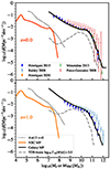 |
Fig. A.1. Stellar mass functions of all galaxies (solid black) and TDE host galaxies with the highest TDE rates (Γtot > 10−5, gray dashed) for the fiducial model at z = 0 and z = 1. The first is compared with compiled mass constraints from Henriques et al. (2015) and Henriques et al. (2020), Baldry et al. (2008), Pérez-González et al. (2008), and Moustakas et al. (2013) (inset legend). With a thin colored line at lower masses, the NSC Mass Function of the fiducial model is plotted at the same redshifts. For comparison, we display the model NSC mass function from Antonini et al. (2015) at z = 0 (Ant15 z = 0). |
In the same plot, we present the NSC mass function at z = 0 (dotted-dashed), which is lower compared to the theoretical predictions of Antonini et al. (2015) by an order of magnitude at lower masses, obviously having a different slope. The number density provided by this function should be a theoretical lower limit to reproduce the TDE rates, yet NSCs without MBHs should also be considered. The model predicts that NSCs do not evolve significantly with redshift from z = 1, as they are tightly related to the nuclear MBHs (that also do not evolve).
At z = 0 the peak at hosts with high rates within M* = 109.5 - 1010.5 M⊙ is directly related to hosting massive NSC MNSC = 107-108 M⊙ and recently seeded (high per-galaxy rates, left panel in Fig. A.1 for NSC distribution) while the evolving tail (M* < 109 M⊙ from z = 1 to z = 0 is from the contribution of intermediate-mass MBHs and smaller NSC (right NSC distribution in Fig. A.1), and systems with TDE rates decaying with time. The model predicts mild redshift evolution, a falsifiable argument with the observations of TDEs up to z = 1 from the forthcoming LSST samples.
Appendix B: Useful definitions for tidal disruption event rate interpretation
An interaction between a massive black hole and a star reaches its proximity zone of less than one tidal radius rt (Eq. 3 in the main text), at fixed masses M• and m* respectively, will result in a variety of outcomes, with different energetics and observable signatures depending on many parameters. How close to the horizon the star is destined to make a passage is of particular importance (Carter & Luminet 1982; Stone et al. 2013; Dai et al. 2015). It is useful to quantify this with the penetration parameter that is defined as

where rp the pericenter of the orbit and

The tidal radius depends on the mass/radius of the star disrupted m* and r* (units of 1 M⊙ and 1R⊙). The coefficient ηTD depends on the polytropic index of the star and is of the order unity (Merritt 2013). Penetration factor values range from βmin = 0.5-0.6 as derived from hydrodynamical simulations (Guillochon & Ramirez-Ruiz 2013) and at which point stars are merely disrupted, to βmax at which point stars enter whole into the MBH’s horizon. Analytical calculation on horizon suppression for a Schwarzchild MBH yields (Kesden 2012; Mummery 2024)
Also, below a value βc the star is not fully disrupted. Therefore, full TDEs in the interval βc < β < βmax while direct captures occur for β > βmax(M•). The rest of the events are found in the interval βmin < βc and are considered partial TDEs. The latter are identified by the re-flaring of their source and less frequently from their differentiation in the fading power law (−9/4 instead of −5/3). Ryu et al. (2020a) has shown that the physical tidal radius at which the star is fully disrupted has both stellar and MBH mass dependence. For disrupted stars of mass 0.3 and 1 M⊙, we adopted
where βc, 0 = 2.0,C0 = 0.166 & βc, 0 = 2.65, C0 = 0.204 respectively. We set the simple form βc, 0(m*) = 1.6(m* + 0.45) and fix C0 = 0.2 for our simple calculations here (although there is not a linear transition between stars with different polytropic indices). For reference, Guillochon & Ramirez-Ruiz (2013) and Mainetti et al. (2017) values from simulations for convective & radiation-dominated stars around a M• = 106 M⊙ MBH translate into βc, 0 = 1.08 & 2.2 when fixing C0 = 0.2 respectively. Note that there is a continuous transition from TDEs to direct captures as βc(m*)→βmax(M•, m*, χ•, t), with the Hills mass being rather a range of values for the distribution of star masses. This transition is computed solely in the analysis here; in the main text TDEs are considered as β > βc = 1 (all stars within the tidal radius are disrupted) with βmax → ∞ for M• < 108 M⊙ (direct captures are not considered separately) and βmax < βc for higher MBH masses (all events are considered direct captures).
The number of orbits per penetration factor bin dN(β)/dβ takes the analytical form of a power law for the full loss-cone regime (the system just started to relax). By assuming uniformity of the orbits over rp gives a power-law dependence of ∝ β−2 (Stone et al. 2020). When the relativistic gravity is taken into account, this power law drops to β−10/3 (Coughlin & Nixon 2022) for maximally spinning MBHs (Kerr metric). Also, we consider the scenario where orbits are distributed uniformly over surface 2πrpdrp and the probability function scales as ∝ β−3 (Bricman & Gomboc 2020). At the empty loss-cone regime (the system has relaxed) there is a weak (logarithmic) dependence of rates on β, so essentially we can assume ∝ β0 for this case. For simplicity, we assume that the distribution of orbits destined to do partial TDEs follows from one of the full TDEs as inferred for the disruption of normal stars from Zhong et al. (2022).
We could then write the fraction of full TDEs as the integral of a power-law probability β−Sβ − 1 in the value intervals mentioned above:
where the generic power law Sβ is in the range Sβ ∈ [1, 2] for our calculations, for a nonempty loss cone (for all types of events). For the empty loss-cone regime, Sβ = −1 and events at all β should be equally rare.
Now, we can estimate a general correction for our calculated rates of full disruption stars to the rate of all disruptions by using Eq.B.3, for the regime where βmin ≫ βc ≫ βmax get that full/total TDE rate converges as fFTDE → (βmin / βc)Sβ. For βmin = 0.6 and M• ≲ 106 M⊙ yields almost invariably25 a correction factor of
![$$ \begin{aligned} 1/f_{\rm FTDE} \in [2,4] \end{aligned} $$](/articles/aa/full_html/2024/09/aa49470-24/aa49470-24-eq36.gif)
for Sβ ∈ [1, 2]. This correction could be applied only to young systems relaxing only for the last < 100 Myr that have not emptied their loss-cone. However, the physics of circularization could be different for TDEs varying in β, especially for the unknown regime of lower MBH masses (Kıroğlu et al. 2023, M• = 102 − 104 M⊙) and the rates may be modified accordingly (Wong et al. 2022). These simulations26 show a critical value greater than the one adopted from studies at M• = 106 M⊙, namely βc ∼ 10 / 3 > 47 / 19.1, making the fraction of full disruptions even smaller and this correction greater. Furthermore, this correction factor can be a few tens (> 1 dex), as demonstrated by the self-consistent work on partial disruption events by Bortolas et al. (2023). By visual inspection, in the optical sample of Yao et al. (2023) there are more than a few light curves that show a re-flaring activity, instead of a monotonic drop of luminosity. Caution should be drawn when comparing model event rates with samples of TDEs. In the case that indeed events with β < 1 are included in the observational sample, the predictions of our model would be > 1dex apart from observations and a more thorough discussion should be done on the optimistic assumptions we made when translating PHASEFLOW rates to observations (see Sect. 2.3.4)
All Figures
|
Fig. 1. Massive black hole mass function (top) and median spin for X-ray bright MBHs (bottom) as a function of the MBH mass M• predicted by the L-Galaxies BH model used in this work. Data are shown for z = 0 (red solid line) and z = 5.5 (yellow dashed line), with shaded areas in the bottom panel referring to the 1σ dispersion at a given mass range. In the top panel, the gray dashed line corresponds to the MBH mass function value equal to 1 dex−1 per MSII simulation volume. The results are compared with observational data at z = 0; MH08, Vika09, Sh09, Cao10, Sh13, Arvs15, GS19, and MuPa16 refer to the model-dependent constraints on the MBH mass function derived respectively by Merloni & Heinz (2008), Cao (2010), Gallo & Sesana (2019), Shankar et al. (2009, 2013), Mutlu-Pakdil et al. (2016), Vika et al. (2009), Aversa et al. (2015). For spin constraints, we display the upper and lower limits from X-ray reflection spectroscopy (Reynolds 2021). For a closer comparison to observational results, the average spin values shown here are for MBHs with a predicted hard X-ray luminosity of log LHX > 40 erg s−1. |
| In the text | |
|
Fig. 2. Nuclear star cluster occupation fraction for our fiducial model as a function of galaxy stellar mass for all galaxies (solid line) and all galaxies hosting an MBH (dashed line). All M* < 109 M⊙ galaxies hosting an MBH have also a 100% probability of hosting an NSC at creation. The data represents the NSC occupation fraction for the Virgo (orange circles), Fornax (white squares), Coma (gray triangles) clusters, and the Local Volume (green rhombuses) as presented in Hoyer et al. (2021). Our model fits the logistic function for NSC occupation at M* < 109.5 M⊙ of the same work (thin gray line). We stress that this agreement occurs naturally from the occupation of MBHs per galaxy (see discussion in Sect. 4.2). |
| In the text | |
|
Fig. 3. Density profiles for different MBHs and the resulting time-dependent TDE rates. Top panels: stellar density profiles for a range of MBH masses as indicated in the inset legend (with the same color coding applying to all panels of the figures). Disks have been assigned nS = 1 Sérsic profiles (solid lines, left), while bulges have nS = 4 profiles (dotted lines, left). The NSCs were instead assigned spheroid profiles from Eq. (9) (right). The galaxy and NSC host properties scale with M• as described in the text and are created to be representative of the average environment encountered in L-Galaxies BH. Middle and bottom panels: tidal disruption event rate evolution with PHASEFLOW when initiating for different MBH mass with the associated profiles from the top panels, displayed separately for bulges or disks (galaxy component, middle panel) and NSCs (bottom). The gray region below 10 Myr indicates the region where we trace unresolved growth and high-rates below the time-resolution dtstep for the black holes in NSCs with mass M• < 106 M⊙. This initial phase we refer to as prompt phase. |
| In the text | |
|
Fig. 4. Flowchart of the current scheme for estimating TDEs within a single time step of L-Galaxies BH. The decision-making tree is colored red and blue for the galaxy (bulge or disk in the absence of bulge) and NSC components, respectively. With the density profile ρgal we refer to all galaxy component parameters {Mgal,Rgal,nS} that are used to initialize the Sérsic profile. TDE rates from the galaxy as a whole and its NSC are effectively treated independently (each process has its clock ΔtTD) and can be active at the same time, while they sum together to produce the instantaneous rate of each MBH. |
| In the text | |
|
Fig. 5. Volumetric TDE rates per black hole (M•, left) and galaxy (M*, right) log mass at z = 0.0 for the fiducial model (solid line). Our model is compared against the constraints (here plotted with the error range) from Yao et al. (2023) for all MBHs (left) and all galaxy types (right). For reference, we display the previous constraints from van Velzen (2018) and the luminosity function from Sazonov et al. (2021) transformed to a mass function (see the details in the text). We also display the model lines of Yao et al. (2023) for the TDE rates as a function of a) MBH mass, assuming the Shankar et al. (2016, maroon shorter dash-dotted line; Sh16) and the Gallo & Sesana (2019, cyan long dash-dotted line; G19) MBH mass functions, which both include the event horizon suppression, and b) galaxy stellar mass, obtained by multiplying the galaxy stellar mass function with the power-law dependence of rates on |
| In the text | |
|
Fig. 6. Average TDE rates per log mass of MBH M• (left) and of the MBH host galaxy M* (right) for the fiducial model at z = 0.0 (solid red line, tagged as “all”). We averaged separately over NSC rates (light-blue lines) and galaxy component rates (maroon lines), and subsequently split into just restarted (“young” systems with ΔtTD < 30 Myr, dashed line) and after a long time (“old” systems with ΔtTD > 3 Gyr, dotted lines). For comparison, we present the results of (Pfister et al. 2020) for three different scaling relation pairs of MBH galaxy stellar mass and NSC mass size adopted in their work (DD, DP, and KD as defined in Table 2 of Pfister et al. 2020) to bracket the uncertainties following these hypotheses. |
| In the text | |
|
Fig. 7. Redshift evolution [z = 0 (top), z = 1 (middle), and z = 2 (bottom)] of the volumetric TDE rates per MBH (left) and stellar (right) mass originating from all low-luminosity or inactive MBHs (cutoff at log10LAGN [erg/s] < 42 for the fiducial model, solid lines) and TDE rates from the galaxy components only bulges (or disks); solid lines tagged as “gal”). We also display the rates only from AGN-hosts with "high" (purple dashed-dotted), "moderate" (green dashed), and “low” (blue dotted) luminosity (log10LAGN [erg/s] ∈ [42, 45], [40.5, 42] and [39, 40.5] respectively). The z = 0 constraints Yao et al. (2023) are plotted in all panels for reference (with gray when they do not apply). These fractions remain qualitatively the same for these redshifts for most of the parameter variations. |
| In the text | |
|
Fig. 8. Average fraction of mass accreted by different MBHs at z = 0 (fBHAM) via stellar captures (purple squares), cold gas accretion (blue right triangles), hot gas accretion (orange left triangles), and accumulated seed mass (green circles) without (top panel) and with (bottom panel) an initial prompt phase (see main text). The margin of ±1 standard deviation of log10fBHAM for each type of channel is highlighted with the same-color shaded area. |
| In the text | |
|
Fig. 9. Variations of the seeding probability in L-Galaxies BH. Top and middle panels: occupation fractions of MBH (M• > 105 M⊙, top) and NSC (all masses, middle) that result into the volumetric TDE rates as a function of galaxy-host mass (bottom). We show the maxOcc and lowOcc models with orange solid and black dashed lines, respectively. In the top panels we display the local MBH occupation fraction derived from a compilation of detections 2012 (2012, cyan squares) and X-ray constraints by Miller & Davies (2012, light-blue region), as well as an occupation for slightly higher redshifts 0.01 < z < 0.1 derived via optical-line AGN Trump et al. (2015, blue circles). In the middle panel, the data points and logistic function (the dashed-dotted thin line), both from Hoyer et al. (2021), have the same meaning as in Fig. 2. The enhanced MBH occupation is still compatible with the observations of the Coma Cluster (gray triangles), even though it yields a greater fraction of nucleated galaxies. We stress that all NSCs are hosting an MBH in our model, hence adding NSCs without MBHs would increase this fraction. Bottom panel: Both maxOcc and lowOcc model (solid and dashed line) reproduce the TDE-rate distribution constraint of Yao et al. (2023) within errors. However, in the lack of evidence of TDEs in dwarf galaxies the lowOcc model is preferred. |
| In the text | |
|
Fig. 10. Volumetric rates at z = 0 per black hole mass (top) and galaxy stellar mass (bottom) for different model variations (names of the models in legend as in text) compared with constraints from Yao et al. (2023, blue shaded area) and the fiducial model (red solid line). The orange shaded area was constructed by assuming no spin and maximally spinning MBHs in the post-processing treatment of the event horizon suppression of the fiducial model (orange solid line). |
| In the text | |
|
Fig. A.1. Stellar mass functions of all galaxies (solid black) and TDE host galaxies with the highest TDE rates (Γtot > 10−5, gray dashed) for the fiducial model at z = 0 and z = 1. The first is compared with compiled mass constraints from Henriques et al. (2015) and Henriques et al. (2020), Baldry et al. (2008), Pérez-González et al. (2008), and Moustakas et al. (2013) (inset legend). With a thin colored line at lower masses, the NSC Mass Function of the fiducial model is plotted at the same redshifts. For comparison, we display the model NSC mass function from Antonini et al. (2015) at z = 0 (Ant15 z = 0). |
| In the text | |
Current usage metrics show cumulative count of Article Views (full-text article views including HTML views, PDF and ePub downloads, according to the available data) and Abstracts Views on Vision4Press platform.
Data correspond to usage on the plateform after 2015. The current usage metrics is available 48-96 hours after online publication and is updated daily on week days.
Initial download of the metrics may take a while.